Enhanced 3D Point Cloud from a Light Field Image

Abstract

The importance of three-dimensional (3D) point cloud technologies in the field of agriculture environmental research has increased in recent years. Obtaining dense and accurate 3D reconstructions of plants and urban areas provide useful information for remote sensing. In this paper, we propose a novel strategy for the enhancement of 3D point clouds from a single 4D light field (LF) image. Using a light field camera in this way creates an easy way for obtaining 3D point clouds from one snapshot and enabling diversity in monitoring and modelling applications for remote sensing. Considering an LF image and associated depth map as an input, we first apply histogram equalization and histogram stretching to enhance the separation between depth planes. We then apply multi-modal edge detection by using feature matching and fuzzy logic from the central sub-aperture LF image and the depth map. These two steps of depth map enhancement are significant parts of our novelty for this work. After combing the two previous steps and transforming the point–plane correspondence, we can obtain the 3D point cloud. We tested our method with synthetic and real world image databases. To verify the accuracy of our method, we compared our results with two different state-of-the-art algorithms. The results showed that our method can reliably mitigate noise and had the highest level of detail compared to other existing methods.

1. Introduction

In order to protect ecosystems, it is necessary to have strong environmental monitoring and reliable 3D information in an agricultural context [1]. The issue of acquiring noiseless and complete 3D point clouds is of paramount importance to support a wide variety of applications such as the 3D reconstruction of buildings [2], precision agriculture, road models and environmental research, which are central in the fields of remote sensing and computer vision. Acquiring 3D data about buildings or monuments in a city can be utilized for the analysis, description and study of 3D city modelling [3]. In fact, 3D information enables us to execute morphological measurements, quantitative analysis, and annotation of information. Moreover, we can generate decay maps, which allow easy access and research on remote sites and constructions. Generating 3D information for crops and plants can also contribute to plant growth and harvest yield quantification for agriculture and production. This is especially relevant to measure the effects of climate change on different land types [4]. The main aim of this work is to create high quality 3D point clouds scanned with one snapshot from real objects for the purpose of having 3D models of buildings, plants or any other real objects for remote sensing and photogrammetry.

A 3D point cloud can be obtained from various methods. Many existing methodologies for reconstruction of 3D models are based on either Structure from Motion (SfM) or Dense Multi-View 3D Reconstruction (DMVR). However, these methods need multiple captures from different angles and significant user interaction when using an ordinary camera. For this reason, recent research has focused on the development of new strategies using less costly devices while continuing to minimize complexity [5].

Given the current state-of-the-art, one very effective solution is to create 3D models from a single image. A single conventional 2D image has limited information about the 3D nature of objects or scenes, so accurate estimation of 3D geometry from a single image is difficult to achieve [6]. Nevertheless, light field images, with the ability to capture rich 3D information with a single capture, offer an effective solution to this problem. The introduction of light field cameras (a type of plenoptic camera) has helped to reveal new solutions and insights into a wide variety of applications, including traditional computer vision, image processing problems and remote sensing research. Light field cameras capture rich information about the intensity, colour and direction of light, and can be used to estimate a depth map or 3D point cloud from a single captured frame. Light field camera technology has the potential to create 3D point cloud reconstructions in circumstances where standard multi-capture techniques can fail, such as dynamic scenes or objects with complicated material appearance. The unique features of light field images—e.g., the capture of light rays from multiple directions—provide the ability to reconstruct 2D images at different focal planes. This feature can also aid in reconstruction of scene depth maps [5]. A light field image can have multiple representations, but two LF representation formats are more common for computer vision and image processing problems; the lenslet format and 4D LF format. In the work we report here, we used the 4D LF format as described below.

For the reconstruction of a 3D point cloud of an object, we developed a new method which is based on the transformation of the point–plane correspondences. The input of our system is a 4D LF image which can be captured by light field cameras, such as the Lytro Illum [7] or created synthetically. The depth map of the LF can be produced by software bundled with the Lytro camera or similar third-party software. Our method is agnostic to the source of the depth map data.

Estimating a densely sampled depth map is essential for creating a 3D point cloud, but the initial depth map provided by commercial LF cameras such as the Lytro Illum is not accurate enough for 3D reconstruction. Figure 1 shows the production of a 3D point cloud from an LF image, based on the proposed method. We devised an approach to enhance the depth map by using an initial LF image as an input image to substantially improve the quality of the recovered depth map. 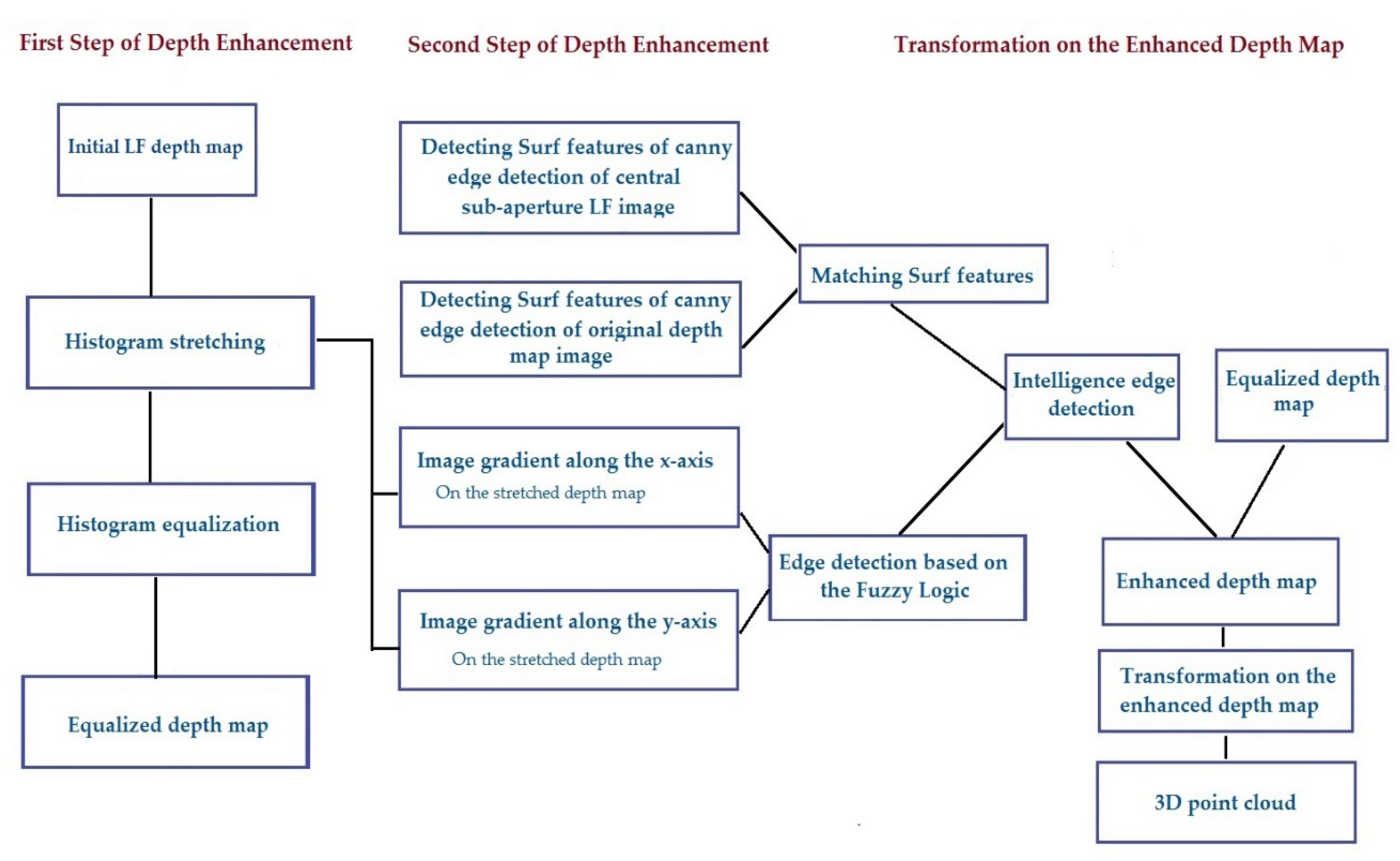Figure 2 shows the detailed block diagram of our proposed method. Specifically, our approach applied histogram equalization and histogram stretching to the initial depth map. We then calculated the gradient of the stretched depth map along the x and y axes separately by comparing the intensity of neighbouring pixels and then, by using a fuzzy logic method, we computationally defined which pixels belonged to the edge of a region of uniform intensity. This kind of edge analysis can improve depth map estimation by leveraging pixel-wise classification, based on their colour mapping properties. In parallel, we detected and extracted Speeded-Up Robust Features (SURF) from Canny edge detection performed on the sub-aperture images of the LF and the original depth map. We then matched features between the edges of the original depth map and the sub-aperture image, and we then added the matched pixels to the edges determined by fuzzy logic analysis. For obtaining the final enhanced depth map, we combined this edge with the equalized depth map by considering the level of the reference image (depth map). We finally transformed the point-plane correspondences to acquire a 3D point cloud.

This proposed non-linear method obtains edges of a depth map and sub-aperture images with greater accuracy than what can be achieved by simply adding linearly the ordinary edge detection information provided by Canny or Sobel filters that alone carry considerably greater noise. Hence, this innovation in the enhancement of the recovered depth map from an LF image is a key contribution of the work we report here.

Our main contributions are:

• We acquire a 3D point cloud based on a single image from a light field camera, which provides valuable information in the field of remote sensing.
• We design a novel approach for enhancing depth maps based on feature matching and fuzzy logic, which can overcome the common problem of introducing noise.
• We develop a method for converting the enhanced depth map to a 3D point cloud.

2. Related Work

Existing 3D reconstruction approaches can be divided into three different groups: methods based on capturing multiple images, creating 3D point clouds based on Deep Learning and approaches based on 3D reconstruction from a single image.

2.1. 3D Reconstruction from Capturing Multiple Images

In general, the reconstruction of 3D point clouds from multiple image captures of the same scene is a computationally expensive process and requires significant user interaction. One of the common methods in this field is Structure from Motion (SfM) which requires the capture of photos of a scene from all feasible angles around the object, especially for fused aerial images and LiDAR (Light Detection and Ranging) data. While the number of images captured with SfM methods is dependent on application, for the same application, a light field approach still has the advantage of needing fewer captures to achieve the same result. In addition, a light field approach has the advantage of working for applications where objects being imaged are dynamic (such as the analysis of plant growth in situ or dynamic urban environments such as streetscapes). Currently such applications represent extreme challenges for SfM approaches. Pezzuolo et al. [8] reconstructed three-dimensional volumes of rural buildings from groups of 2D images by using SfM methods. For working on unmanned aerial vehicle (UAV) images, Weiss et al. [9] utilized RGB colour model imagery for describing vineyard 3D macrostructure based on the SfM method. Bae et al. [10] proposed an image-based modelling technique as a faster method for 3D reconstruction. For image capture, they utilized cameras on mobile devices. One of the benefits of using image-based modelling is the accessibility of texture information that can enable material recognition and 3D Computer-Aided Design (CAD) model object recognition [11,12]. Moreover, some works used the reconstruction of 3D scene geometry for the purpose of control and management of energy in the field of 3D modelling of buildings [13]. Pileun et al. [14] estimated the positions and orientations of the object by using Simultaneous Localization and Mapping (SLAM). The 2D localization information is utilized for creating 3D point clouds. This reduces the time of scanning and requires less effort for collecting accurate 3D point cloud data but still needs user interaction.

2.2. Creating 3D Point Clouds Based on Deep Learning Techniques

Recently, approaches based on deep learning have drawn attention for solving many computer vision problems. A wide variety of deep learning models have been developed to create 3D point clouds but most of them require images capturing an object with an uncluttered background and a fixed viewpoint [15]. Current techniques have limited application to real world objects. Yang et al. [16] generated a point cloud based on a specific deep model named PointFlow. This model has the advantage of having two levels of continuous flows for normalizing the point cloud. The first level is for creating the shape and the second level is for distributing the points. For handling large scale 3D point clouds, Wang et al. [17] developed a method based on the feature description matrix (FDM), combining traditional feature extraction with a deep learning approach. As deep learning alone is not efficient for creating a 3D point cloud, Vetrivel et al. [18] combined a convolutional neural networks approach with 3D features to improve results. Wang et al. [19] used deep learning for fast segmentation of 3D point clouds. They introduced a new framework called Similarity Group Proposal Network (SGPN). However, this method is still not efficient for real world objects.

2.3. 3D Reconstruction from a Single Image Approaches

Creating 3D point clouds from a single image has received significant attention from the research community. However, 3D reconstruction from a single projection still has many problems and is a challenging topic. Mandika et al. [20] estimated 3D point clouds from a single input view by training an auto-encoder to learn a mapping from 2D input images to 3D point clouds. However this type of estimate is not very accurate and requires extensive training [21]. To overcome the drawbacks of estimation of 3D point clouds from a single capture, light field cameras have been proposed. Using light field images as an input can lead to 3D point cloud estimates with low cost and complexity. Perra et al. [5] used light field images as an input image to determine depth maps of scenes and then estimated 3D point clouds. The depth maps that are automatically acquired from light field cameras have some potential limitations when dealing with real objects such as having decreased efficiency and accuracy for dense scenes. To tackle this problem, we propose a novel algorithm for enhancing the depth map by adding multi-modal edge detection information, which provides more information about the depth map. Moreover, compared to the Perra et al. [5] method, we used a transformation method for converting the depth map to 3D, which is more reliable and does not need the segmentation and extraction of occlusion masks required by their method.

2.4. Problems of Existing Approaches and Our Solution

Each of the three aforementioned method types have some limitations for creating dense and accurate 3D point clouds and most of them require considerable effort to obtain 3D data. Methods that make use of multiple images, such as SfM and SLAM, usually require finely textured objects without specular reflections. Moreover, if the baselines used for separating the viewpoints are chosen to be large, it causes many problems for feature correspondences on account of occlusion and changes in local appearance [15]. For deep learning approaches, despite the recent favourable results of deep learning models in some machine learning tasks, creating 3D point clouds remains challenging [16]. This difficulty can be attributed to the lack of order in the 3D point cloud, so no static structure of the topology can be found for recognition and classification of the scene based on the deep learning. This means it will be problematic to use deep neural networks directly on the point clouds because points will not be arranged in a stable order like pixels are in 2D images.

Many attempts have been made to address the problem of 3D reconstruction from a single snapshot, however, when those methods are applied on real images, they will suffer from a sparsity of information. Since in the one snapshot there will be a single view of the image, some parts of the scene will therefore be invisible. This shortage causes the generation of 3D point clouds to be problematic. In contrast, we used a light field camera in this work, which by one snapshot provides multiple sub-aperture images, providing sufficient data for depth map estimation. As a result, compared to other single image methods, we can overcome the problem of this kind of deficiency. Moreover, we enhanced the depth map in a novel, multi-modal fashion by extracting SURF features from central sub-aperture matching and depth map images, and using fuzzy logic. This kind of enhancement provides for our work a more accurate point cloud compared to other methods in this area, and also makes the reconstruction of 3D point clouds much easier.

3. The Light Field Camera

In the field of environmental research, there are a wide variety of techniques trying to obtain 3D information about buildings and plants. Most of the previous techniques needed a high level of methodological complexity, but with the emergence of light field cameras, many problems have now been addressed in the areas of 3D modelling, measurement and monitoring. A light field camera, which is a type of plenoptic camera that with one image capture through an array of micro-lenses, can collect a wide variety of information about the colour, intensity and direction of light in a scene. This means, instead of utilizing two or more single camera captures to increase the number of viewpoints, light field cameras provide many viewpoints of a scene with a single snapshot and each such view is termed a “sub-aperture image”. In contrast, in a traditional digital camera, the lack of data about the directional intensity of light makes solving many problems of remote sensing and computer vision difficult. An early light field camera was developed in 2005 and was called the Lytro [7], and a professional version of the Lytro was introduced in 2014 (called the Lytro Illum). Light field cameras have several features such as post-capture refocusing, depth map estimation and illumination estimation. In the field of remote sensing, light field cameras are also suitable for generating 3D information for different kinds of monitoring applications, such as the monitoring of plant growth [1].

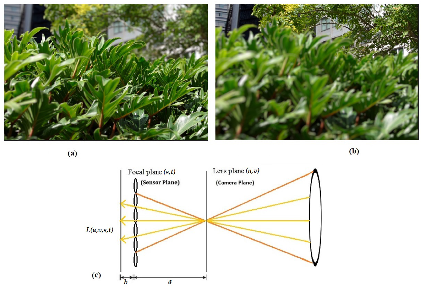
One of the significant features of light field cameras is shown in Figure 3, which shows post-capture refocusing in two different focal planes. Refocusing allows for changing the focal plane to a different position post-capture. This feature has a significant role in the generation of a depth map from a LF image. A light field can be considered as a vector function I(u, v, s, t) between two planes (lens plane and sensor plane) [22] where u and v are coordinates on the lenses plane and s and t are co-ordinates on the sensor plane as shown in Figure 3.

An aligned light ray is determined in a system when it first crosses the uv plane (lens plane) at coordinate (u, v) and then crosses the st plane (sensor plane) at coordinate (s, t), and can be encoded by the function of I(u, v, s, t) [22]. Each position on the sensor plane can be modelled as a pinhole camera viewing the scene from a position s, t on the sensor plane.

4. Proposed Method

In this work, we used a LF image and its depth map as an input image. Our approach is based on transforming the point–plane correspondences on an enhanced depth map. Since having an accurate depth map is of paramount importance to generate a complete 3D point cloud, we improved the depth map in two different steps. In the first step, we applied histogram stretching and equalization on the original depth map. In the second step of enhancement, we added multi-modal edge detection information to the equalized depth map, then we acquired the 3D point cloud by coordinate transformation.

4.1. Histogram Stretching and Equalization

In the first step of enhancement, we applied histogram stretching and equalization on the original depth map as one of the novel aspects of this work. Our input was an 8-bit grayscale 2D depth map image, $DM\left(u,v\right)$. In order to increase the distance between adjacent depth layers, we applied histogram stretching and then on the result of the histogram stretching, we applied histogram equalization. The equations below show the histogram stretching to improve the separation between the depth planes.

$$m_{uv}=\frac{D{M}_{max}-D{M}_{min}}{255}$$

(1)

$$b_{uv}=255-m_{uv}\ast D{M}_{max}$$

(2)

$$H{S}_{uv}=m_{uv}\ast D{M}_{uv}+b_{uv}$$

(3)

where $D{M}_{uv}$ is a 2D depth map image with a minimum value denoted as $D{M}_{min}$ and a maximum value denoted as $D{M}_{max}$ and $H{S}_{uv}$ is the histogram stretched depth map. Then, we applied histogram equalization on the result of the histogram stretching to spread the intensity values over full range of the histogram image and for enhancing the contrast of the depth map [23].

Given the histogram stretched depth map $H{S}_{uv}$, if we consider $r_k$ as the dynamic range of intensities in the depth map, then the probability based on the histogram $p(r_k)$ can be calculated as below:

$$p(r_k)=\frac{Total pixels with intensity r_k }{Total pixel in depth map H{S}_{uv}}$$

(4)

From this probability we can perform histogram equalization based on the below equation:

$$H{Q}_{uv}={\displaystyle \sum }_{k=0}^{n}p(r_k)$$

(5)

where $n$ is the number of pixels and $H{Q}_{uv}$ is the result of histogram equalization.

4.2. Adding Edge Detection Information

The second step of enhancement was the most important part, where we added multi-modal edge detection information. This is another significant and novel aspect of this work. We developed a new strategy in this area, making use of the fuzzy logic-based edge information created from the depth map and feature correspondence matching between sub-aperture images to create a multi-modal edge estimation. This information was then combined to obtain a multi-modal edge detection. As a result, this kind of edge detection was more reliable compared to ordinary edge detection because noise was reduced compared to prior art edge detection methods such as Canny and Sobel. This means we determined edges efficiently in a multi-model fashion, based on the depth map in conjunction with the sub-aperture images, rather than selecting any edge which was created by current state-of-the-art edge detection methods working on the sub-aperture images alone. The details of this development are shown in Figure 4 and Figure 5, which also show the steps required for improvement of the depth map.

4.2.1. Fuzzy Logic

We found that a fuzzy logic approach can help us with detecting edges by comparing the intensity of neighbouring pixels, and based on the gradient of the image, we can find which pixels belong to an edge. This kind of logic is very helpful for depth map images because of the structure of level of depth map is based on the gradients.

We first obtained the image gradients based on the convolution of the image to acquire a matrix containing the u-axis and v-axis gradients of the depth map image.

For this purpose, we convolved the depth map $H{S}_{uv}$ with gradient operator,$$, using the convolution method. The gradient values were in the [−1 1] range.

$$Gx=\left[-1 1\right], Gy=G\acute{x}$$

(6)

$$G_{uv}={\displaystyle \sum }_u{\displaystyle \sum }_{v}HS\left(u,v\right)G{\left(x-u+1,y-v+1\right)}_{ }$$

(7)

Considering the gradients of the depth map as an input, we will create a fuzzy inference system (FIS) for edge detection.

FIS is made based on the decision of whether a pixel is belonging to an edge or not. Membership functions are needed to define a fuzzy system. We defined a Gaussian membership function for each input:

$${\mu }_{uv}=Gaussian\left(G_{uv}\right)=e^{[-{\left(G_{max}-G_{min}\right)}^2/2{\sigma }^2]}$$

(8)

where ${\mu }_{uv}$ is a Gaussian function, $G_{max}$, $G_{min}$ are the maximum and minimum value of gradient and $\sigma$ is the standard deviation associated with the input variable.

$F_{uv}$ defines the final pixel classification as edge or non-edge.

$$F_{uv}=\frac{{{\displaystyle \sum }}_{u,v}{\partial }_c{\mu }_{uv}\left({\partial }_{uv}\right)}{{{\displaystyle \sum }}_{u,v}{\mu }_{uv}\left({\partial }_{uv}\right)}$$

(9)

where ${\partial }_{uv}$ are the fuzzy sets as a part of a fuzzy rule, similar to [24] and ${\partial }_c$ is the output class centre of fuzzy rule. As a result, the final fuzzy edge is defined by $F_{uv}$ where 0 indicates that the pixel is almost certainly not part of an edge and 1 indicates that the pixel is almost certainly part of an edge.

4.2.2. Feature Matching

In the second step of enhancement we also in parallel extracted the SURF features of intermediate results $CS{A}_{uv}$ (Canny edge detection for the central sub-aperture image) and $CD{E}_{uv}$ (Canny edge detection of original depth map). Then, we matched the features and extracted features with higher amplitude to add to the result of the edge detection using fuzzy logic.

For this purpose, we used the SURF detector for detecting features. The SURF detector extracts features based on the Hessian matrix, which is determined at any point $\mathrm{po}=\left(u,v\right)$ and scale σ=1.2 as the second order derivative of Gaussian filter.

$$H_{approx}\left(\mathrm{po},\mathsf{\sigma }\right)=\left[\begin{array}{cc}{D}_{uu}\left(\mathrm{po},\mathsf{\sigma }\right)& D_{uv}\left(\mathrm{po},\mathsf{\sigma }\right)\\ D_{uv}\left(\mathrm{po},\mathsf{\sigma }\right)& D_{vv}\left(\mathrm{po},\mathsf{\sigma }\right)\end{array}\right]$$

(10)

where $D_{uu}\left(\mathrm{po},\mathsf{\sigma }\right),D_{uv}\left(\mathrm{po},\mathsf{\sigma }\right),D_{vv}\left(\mathrm{po},\mathsf{\sigma }\right)$ are the convolution of the Gaussian second order at the point of $\mathrm{po}=\left(u,v\right)$. This can be executed methodically if utilizing an integral image, as a result we calculate the integral image for those two input images:

$$CSA\left(u,v\right)={\displaystyle \sum }_{0\le i\le u} {\displaystyle \sum }_{0\le j\le v}CSA\left(i,j\right)$$

(11)

$$CDE\left(u,v\right)={\displaystyle \sum }_{0\le i\le u} {\displaystyle \sum }_{0\le j\le v}CDE\left(i,j\right)$$

(12)

The determinant of approximate Gaussians can be presented as follows:

$$det\left(H_{approx}\right)=D_{uu}{D}_{vv}-{\left(0.9D_{uv}\right)}^2$$

(13)

Therefore, the interest points, which includes their locations and scales, will be detected in approximate Gaussian scale space [25].

For matching the features of those two images, we used the nearest neighbour method similar to [25]. In this way, image $CS{A}_{uv}$ has $n_1$ directed line segments and image $CD{E}_{uv}$ has $n_2$ directed line segments, and the nearest neighbour pair can be obtained by defining matrix K as below:

$$K\left(i,j\right)=\{\begin{array}{c}1 \mathrm{CSA} \mathrm{is} \mathrm{the} \mathrm{nearest} \mathrm{neighbor} \mathrm{of} \mathrm{CDE} \\ 0 otherwise \end{array}$$

(14)

Then, we determined the features point with the highest amplitude from $K\left(i,j\right)$.

At the end of this step, we added the result of feature matching to the edge of fuzzy logic. As a result, we will have a multi-modal edge detection that we called $In{t}_{uv}$.

$$In{t}_{uv}=\left|F_{uv}\right|+\left|K_{uv}\right|$$

(15)

In the next step, we added this edge detection to the equalized depth map by applying a median filter, and the result will be saved in $T_{uv}.$

$$T_{uv}=Adding\left[ In{t}_{uv} and H{Q}_{uv}\right]$$

(16)

4.3. Creating 3D Point Cloud by Transforming the Point-Plane Correspondences

For estimation of the 3D point cloud, we needed to estimate $T_z$ (the z component of each point at position u,v) from which a point cloud can be created by transforming the point–plane.

For the points in the final point cloud, we started by selecting $T_x=T_u$ and $T_y=T_v$, then for computing $T_z$:

$$D=b\ast fl\ast fc$$

(17)

$$T_z=\frac{D}{T_{xy}\ast fc\ast b\ast \max \left(T_{xy}\right)}$$

(18)

where $b$ is amount of the baseline, $fl$ is the focal length and $fc$ is the focus distance. The variable $fl$ is an intrinsic parameter and depends on the captured image. The variables $b$ and $fc$ are extrinsic parameters and depend on the type of camera. The x and y coordinates of the point are then given by:

$$\acute{{\mathrm{T}}_x}=\frac{{\mathrm{T}}_x\ast T_z}{Se}$$

(19)

$$\acute{{\stackrel{´}{T}}_y}=\frac{{\mathrm{T}}_y\ast T_z}{Se}$$

(20)

where $Se$ is the sensor size (mm). We then denote the estimation of 3D point cloud by $T_{xyz}$:

$$T_{xyz}=\left({\acute{T}}_x ,{\acute{T}}_y,T_z\right)$$

(21)

5. Experimental Results

We evaluated our method with three different databases and compared the proposed method with two state-of-the-art methods, as described in further detail below. For assessing the accuracy of our proposed method numerically, we used two different metrics: Histogram Analysis and LoD (Level of Details), as shown in part 5.3.

5.1. Result on Databases

We utilized three different databases: one synthetic database and two real world light field image databases. We tested our method with several images. For the synthetic database, we used a database popularized by the research community, which was created by Honauer et al. [26]. For the real world image databases, we used the real world LF database from JPEG (JPEG Pleno Database) [27], which includes the result of their depth map estimation. We also used a third custom database of images acquired using a Lytro Illum. For a more comprehensive evaluation, we captured images in different situations, including images with shading, low-texture, and challenging images such as very bright images and images with occluded pixels. Our method was tested on a wide variety of images, of which, a sample of results on synthetic images is shown in Figure 1. Figure 5 and Figure 6 are based on the JPEG database. Figure 7 shows the result for images we captured using a Lytro Illum camera. Figure 8 is another sample of JPEG database.

5.2. Methods Compared

To illustrate the accuracy of our proposed method, we compared our result with the methods of Perra et al. [5] and Dansereau et al. [28] for creating 3D point clouds based on depth maps. As shown in Figure 7 and Figure 8, we compared the output by our method with their data. We re-implemented the method of Perra et al. in Matlab to compare its performance with our result. As seen in Figure 7 and Figure 8, because Perra et al. used Sobel edge detection for modifying their depth map, this kind of edge detection will cause noise that appears as blue pixels in the image. For Dansereau et al. [28], we also re-implemented just the 3D reconstruction part of their method in Matlab and evaluated their result against ours. Another comparison on a challenging image is shown in Figure 7. We captured this image with a Lytro Illum camera.

5.3. Evaluation Methods

For evaluating the performance of 3D point cloud algorithms, we used two different metrics: Histogram Analysis and Level of Details (LoD). These metrics assess the accuracy of a 3D point cloud by considering two important factors—density and distribution [29]. In this way, by analysing the histogram we can assess the range of distance values of the 3D point cloud distribution and by measuring LoD, we can evaluate the range of densities. We describe each part below:

Histogram Analysis: One significant factor for assessing the accuracy of the 3D point cloud is evaluating the distribution of positions of pixels in the 3D point cloud by analysing the histogram [29,30]. A histogram of an image is a plot that indicates the distribution of intensities in an image. For a point cloud, this concept can be extended to indicate the distribution of positions of points in the point cloud. Ideally, for a dense, natural scene, the histogram of positions should have an even, flat distribution, indicating details evenly distributed across all depths and directions. To compute histogram statistics, we calculate the histogram of our 3D point cloud as well as histograms of two other state-of-the-art methods. To increase the accuracy of the evaluation, we measured the histogram of the 3D point cloud based on each dimension (X, Y and Z) along with the mean and standard deviation. Figure 9 shows the histogram of 3D point clouds for the three different methods for a light field image that is captured by a Lytro camera (Green. Figure 7). These histograms indicate the number of pixels in the image at each different value of position relative to the centre of the viewpoint. In Figure 9, the first part (a) corresponds to the histograms which are obtained from our 3D point cloud, and it is clear that the range of positions of our 3D point cloud is higher and more evenly distributed than the other methods compared, especially in the Z dimension.

In Figure 9b, the histograms from Perra et al. [5] are shown, which have a more even distribution of positions compare to Dansereau et al. [28]. As a result, based on the histogram analysis, we can confirm that for the factor of distribution, our 3D point cloud provides more favourable distribution of positions compared to the two other methods.

Level of Details: One of the significant factors for evaluating the amount of density of a 3D model is measuring the level of detail [31]. In computer graphics, the level of detail is defined as the number of vertices (or faces) that generate an object. The level of detail influences the density of the 3D model [31]. Therefore, having a higher number of vertices or surfaces means having higher density, which creates a more complex and potentially informative surface [5]. Moreover, sometimes level of detail is utilized to indicate the number of needed polygons for describing an object. The information about the LoD will be obtained from the 3D mesh. For this purpose, we write the 3D point cloud to PLY (Polygon File Format) format for the calculation of mesh data. Then, we calculated the number of vertices and surfaces for each object. For comparing the LoD of our 3D point cloud with the two other state-of-the-art methods, we have chosen some light field images as an input and after converting the 3D point cloud to PLY format, we obtained the LoD properties.

Table 1. Numerical evaluation of 3D point cloud based on LoD ([number of vertices], [number of faces]).

Light Field Image	Perra et al. [5]	Dansereau et al. [28]	Our Method
Buildings-Black-fence. Figure 8	[65,264] a, [12,6970] b	[62,215] a, [123,056] b	[70,568] a, [139,452] b
Nature-Flowers. Figure 6	[84,729] a, [165,584] b	[72,980] a, [141,069] b	[98,245] a, [192,874] b
Green. Figure 7	[72,548] a, [142,309] b	[73,415] a, [145,977] b	[82,579] a, [161,231] b

^a number of vertices, ^b number of faces.

shows the result of LoD information for the three different 3D model of light field images. It can be seen that the result of our method produced a higher number of vertices and faces compared to the two other methods. As a result, our method can create a denser 3D point cloud. We have done this experiment in several light field images and in all experiments, the amount of density in our method was higher than those two methods. It should be noted that LoD can be increased by the addition of noise, however the results of the histogram analysis in the previous section show that our approach produces a more even distribution of point cloud positions, which is not what one would expect if our approach was simply noisier than other approaches.

6. Discussion

The experimental results were evaluated visually and statistically, as explained in Section 5. We tested our method with several light field images and from the results we can show that our 3D point cloud is more accurate and has less noise due to our modification of the depth map in two different steps. We solved the problem of pixel distribution in the first step of the modification by using histogram stretching and equalization. Furthermore, we solved the problem of density by using special edge detection compared to using any current state-of-the-art methods for adding edges. We showed that by using fuzzy logic we could choose some special edges in a multi-modal fashion by comparing the intensity of neighbouring pixels. Our proposed approach is also novel because it employs parallel processing to improve what is conventionally achieved in generating a raw depth map from the Lytro camera. Unlike previous methods, the method involves a dual-enhancement approach that first computes the fuzzy logic orientation field computed from the histogram equalized sum of depth map and central sub-aperture images. The alternative phase of our approach is to determine the Canny edge response to the central sub-aperture image and the LF depth map, which are then computed for SURF features and combined together through feature matching and merged with the result of the first orientation field computation phase. This newly proposed approach was found here to generate 3D point clouds for the purpose of remote sensing which were superior in detail and clarity, compared with the conventional approaches for generating a 3D point cloud from the depth map of a LF alone.

7. Conclusions

We have generated a 3D point cloud based on one light field image. For this purpose, we propose a modified two-step depth map approach for increasing the accuracy of the depth map estimation for the generation of a 3D point cloud by transformation of the point–plane correspondences. In the first step, we used histogram stretching and equalization which can improve the separation between the depth planes, and in the second step, we developed a new strategy for adding multi-modal edge detection information to the previous step using fuzzy logic and feature matching. In this work, we utilized a light field camera which can be useful for remote sensing applications such as generating a 3D point cloud for agriculture monitoring and monitoring of plant growth. We have chosen our images of buildings and plants to show some applications of our work in the area of remote sensing and environmental research. The results confirm that our method can generate 3D point clouds with improved accuracy compared to other state-of-the-art methods, and our modified depth map ensures an improved result. In future work, we will consider the performance of our model using objects with complicated material appearances which are more challenging to scan into 3D point clouds.

References

1. Schima, R.; Mollenhauer, H.; Grenzdörffer, G.; Merbach, I.; Lausch, A.; Dietrich, P.; Bumberger, J. Imagine all the plants: Evaluation of a light-field camera for on-site crop growth monitoring. Remote Sens. 2016, 8, 823. [Google Scholar] [CrossRef] [Green Version]
2. Zhang, J.; Lin, X.; Ning, X. SVM-based classification of segmented airborne LiDAR point clouds in urban areas. Remote Sens. 2013, 5, 3749–3775. [Google Scholar] [CrossRef] [Green Version]
3. Grilli, E.; Remondino, F. Classification of 3D Digital Heritage. Remote Sens. 2019, 11, 847. [Google Scholar] [CrossRef] [Green Version]
4. Mesas-Carrascosa, F.-J.; de Castro, A.I.; Torres-Sánchez, J.; Triviño-Tarradas, P.; Jiménez-Brenes, F.M.; García-Ferrer, A.; López-Granados, F. Classification of 3D point clouds using color vegetation indices for precision viticulture and digitizing applications. Remote Sens. 2020, 12, 317. [Google Scholar] [CrossRef] [Green Version]
5. Perra, C.; Murgia, F.; Giusto, D. An analysis of 3D point cloud reconstruction from light field images. In Proceedings of the 2016 Sixth International Conference on Image Processing Theory, Tools and Applications (IPTA), Oulu, Finland, 12–15 December 2016; pp. 1–6. [Google Scholar]
6. Li, K.; Pham, T.; Zhan, H.; Reid, I. Efficient dense point cloud object reconstruction using deformation vector fields. In Proceedings of the European Conference on Computer Vision (ECCV), Munich, Germany, 8–14 September 2018; pp. 497–513. [Google Scholar]
7. Ng, R.; Levoy, M.; Brédif, M.; Duval, G.; Horowitz, M.; Hanrahan, P. Light field photography with a hand-held plenoptic camera. Comput. Sci. Tech. Rep. CSTR 2005, 2, 1–11. [Google Scholar]
8. Pezzuolo, A.; Giora, D.; Sartori, L.; Guercini, S. Automated 3D reconstruction of rural buildings from structure-from-motion (SfM) photogrammetry approach. In Proceedings of the International Scientific Conference, Jelgava, Latvijas, 23–25 May 2018. [Google Scholar]
9. Weiss, M.; Baret, F. Using 3D point clouds derived from UAV RGB imagery to describe vineyard 3D macro-structure. Remote Sens. 2017, 9, 111. [Google Scholar] [CrossRef] [Green Version]
10. Bae, H.; White, J.; Golparvar-Fard, M.; Pan, Y.; Sun, Y. Fast and scalable 3D cyber-physical modeling for high-precision mobile augmented reality systems. Personal Ubiquitous Comput. 2015, 19, 1275–1294. [Google Scholar] [CrossRef]
11. Dimitrov, A.; Golparvar-Fard, M. Vision-based material recognition for automated monitoring of construction progress and generating building information modeling from unordered site image collections. Adv. Eng. Inform. 2014, 28, 37–49. [Google Scholar] [CrossRef]
12. Kim, C.; Kim, B.; Kim, H. 4D CAD model updating using image processing-based construction progress monitoring. Autom. Constr. 2013, 35, 44–52. [Google Scholar] [CrossRef]
13. Jarząbek-Rychard, M.; Lin, D.; Maas, H.-G. Supervised detection of façade openings in 3D point clouds with thermal attributes. Remote Sens. 2020, 12, 543. [Google Scholar] [CrossRef] [Green Version]
14. Kim, P.; Chen, J.; Cho, Y.K. SLAM-driven robotic mapping and registration of 3D point clouds. Autom. Constr. 2018, 89, 38–48. [Google Scholar] [CrossRef]
15. Xia, Y.; Wang, C.; Xu, Y.; Zang, Y.; Liu, W.; Li, J.; Stilla, U. RealPoint3D: Generating 3D point clouds from a single image of complex scenarios. Remote Sens. 2019, 11, 2644. [Google Scholar] [CrossRef] [Green Version]
16. Yang, G.; Huang, X.; Hao, Z.; Liu, M.-Y.; Belongie, S.; Hariharan, B. Pointflow: 3d point cloud generation with continuous normalizing flows. In Proceedings of the IEEE International Conference on Computer Vision, Seoul, Korea, 27 October–2 November 2019; pp. 4541–4550. [Google Scholar]
17. Wang, L.; Meng, W.; Xi, R.; Zhang, Y.; Ma, C.; Lu, L.; Zhang, X. 3D point cloud analysis and classification in large-scale scene based on deep learning. IEEE Access 2019, 7, 55649–55658. [Google Scholar] [CrossRef]
18. Vetrivel, A.; Gerke, M.; Kerle, N.; Nex, F.; Vosselman, G. Disaster damage detection through synergistic use of deep learning and 3D point cloud features derived from very high resolution oblique aerial images, and multiple-kernel-learning. ISPRS J. Photogramm. Remote Sens. 2018, 140, 45–59. [Google Scholar] [CrossRef]
19. Wang, W.; Yu, R.; Huang, Q.; Neumann, U. Sgpn: Similarity group proposal network for 3d point cloud instance segmentation. In Proceedings of the IEEE Conference on Computer Vision and Pattern Recognition, Salt Lake City, UT, USA, 18–23 June 2018; pp. 2569–2578. [Google Scholar]
20. Mandikal, P.; Murthy, N.; Agarwal, M.; Babu, R.V. 3D-LMNet: Latent embedding matching for accurate and diverse 3D point cloud reconstruction from a single image. arXiv 2018, arXiv:1807.07796. [Google Scholar]
21. Hong, D.; Yokoya, N.; Chanussot, J.; Zhu, X.X. Cospace: Common subspace learning from hyperspectral-multispectral correspondences. IEEE Trans. Geosci. Remote Sens. 2019, 57, 4349–4359. [Google Scholar] [CrossRef] [Green Version]
22. Wu, G.; Masia, B.; Jarabo, A.; Zhang, Y.; Wang, L.; Dai, Q.; Chai, T.; Liu, Y. Light field image processing: An overview. IEEE J. Sel. Top. Signal Process. 2017, 11, 926–954. [Google Scholar] [CrossRef] [Green Version]
23. Abubakar, F.M. Image enhancement using histogram equalization and spatial filtering. Int. J. Sci. Res. (IJSR) 2012, 1, 105–107. [Google Scholar]
24. Aborisade, D. Fuzzy logic based digital image edge detection. Glob. J. Comput. Sci. Technol. 2010, 10, 78–83. [Google Scholar]
25. Yang, Z.; Shen, D.; Yap, P.-T. Image mosaicking using SURF features of line segments. PLoS ONE 2017, 12, e0173627. [Google Scholar] [CrossRef] [Green Version]
26. Honauer, K.; Johannsen, O.; Kondermann, D.; Goldluecke, B. A dataset and evaluation methodology for depth estimation on 4D light fields. In Proceedings of the Asian Conference on Computer Vision, Taipei, Taiwan, 20–24 November 2016; pp. 19–34. [Google Scholar]
27. Rerabek, M.; Ebrahimi, T. New light field image dataset. In Proceedings of the 8th International Conference on Quality of Multimedia Experience (QoMEX), Lisbon, Portugal, 6–8 June 2016. [Google Scholar]
28. Dansereau, D.G.; Mahon, I.; Pizarro, O.; Williams, S.B. Plenoptic flow: Closed-form visual odometry for light field cameras. In Proceedings of the 2011 IEEE/RSJ International Conference on Intelligent Robots and Systems, San Francisco, CA, USA, 25–30 Septemer 2011; pp. 4455–4462. [Google Scholar]
29. Harwin, S.; Lucieer, A. Assessing the accuracy of georeferenced point clouds produced via multi-view stereopsis from unmanned aerial vehicle (UAV) imagery. Remote Sens. 2012, 4, 1573–1599. [Google Scholar] [CrossRef] [Green Version]
30. Chen, J.; Mora, O.; Clarke, K. Assessing the accuracy and precision of imperfect point clouds for 3d indoor mapping and modeling. ISPRS Ann. Photogramm. Remote Sens. Spatial Inf. Sci. 2018, 4, 3–10. [Google Scholar] [CrossRef] [Green Version]
31. Koutsoudis, A.; Vidmar, B.; Ioannakis, G.; Arnaoutoglou, F.; Pavlidis, G.; Chamzas, C. Multi-image 3D reconstruction data evaluation. J. Cult. Herit. 2014, 15, 73–79. [Google Scholar] [CrossRef]
Figure 1. Using a light field image for creating a 3D point cloud.
Remotesensing 12 01125 g001
Figure 2. A block diagram of our approach.
Remotesensing 12 01125 g002
Figure 3. An illustration of the light field function and post-capture re-focusing. (a) Focus in the foreground. (b) Focus in the background. (c) A diagram of a light field camera setup where a is the distance from the camera plane to the sensor plane and b is the distance between the sensor and the micro-lens array.
Remotesensing 12 01125 g003
Figure 4. Details of our proposed 3D point cloud estimation method.
Remotesensing 12 01125 g004
Figure 5. Steps of modifying the depth map.
Remotesensing 12 01125 g005
Figure 6. Obtaining a 3D point cloud based on the JPEG real world light field image (Nature-Flowers).
Remotesensing 12 01125 g006
Figure 7. Comparing our result with other state-of-the-art methods. This input light field image is captured by ourselves with a Lytro Illum camera.
Remotesensing 12 01125 g007
Figure 8. Comparing our result with other state-of-the-art methods. This input light field image is one of the JPEG database that is a real world LF image (Buildings-Black fence).
Remotesensing 12 01125 g008
Figure 9. Comparing the histogram of our result with other state-of-the-art methods for image Green (Figure 7). (a) Shows the histograms obtained from our 3D point cloud method. (b) Indicates the histograms of Perra et al. [5] method for creating 3D point cloud and (c) shows the result of Dansereau et al. [28]. From the figure it is obvious that the histograms of our method (a) have a more favourable distribution of positions, especially in Z dimension, compared to the two other methods.
Remotesensing 12 01125 g009