GHS-POP Accuracy Assessment: Poland and Portugal Case Study


Abstract
1. Introduction
2. Materials and Study Area
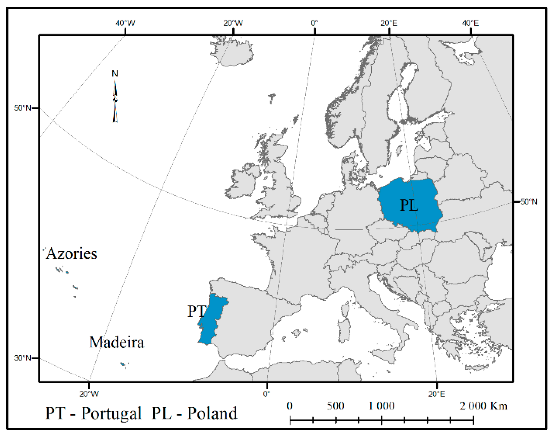
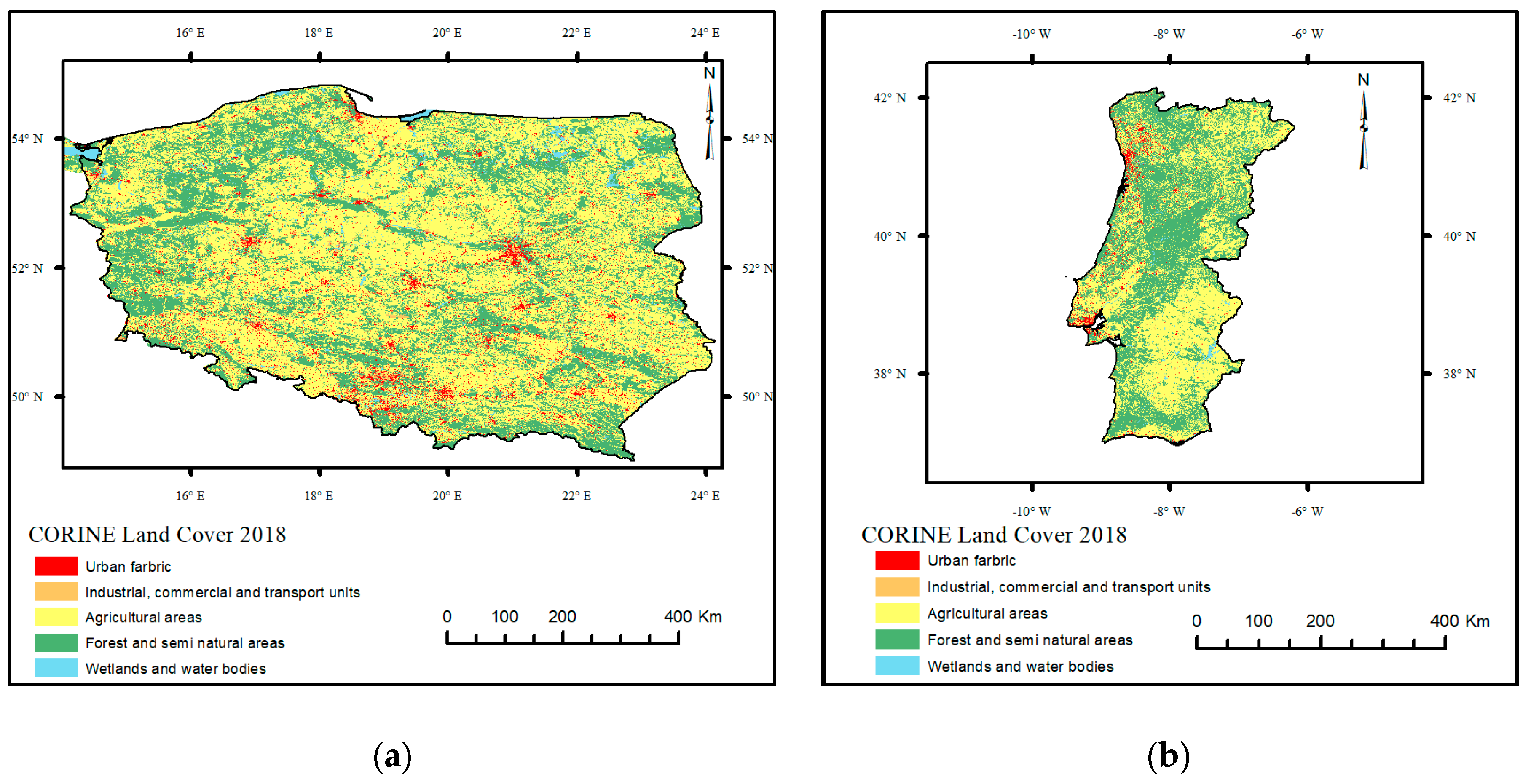
2.1. Poland and Portugal
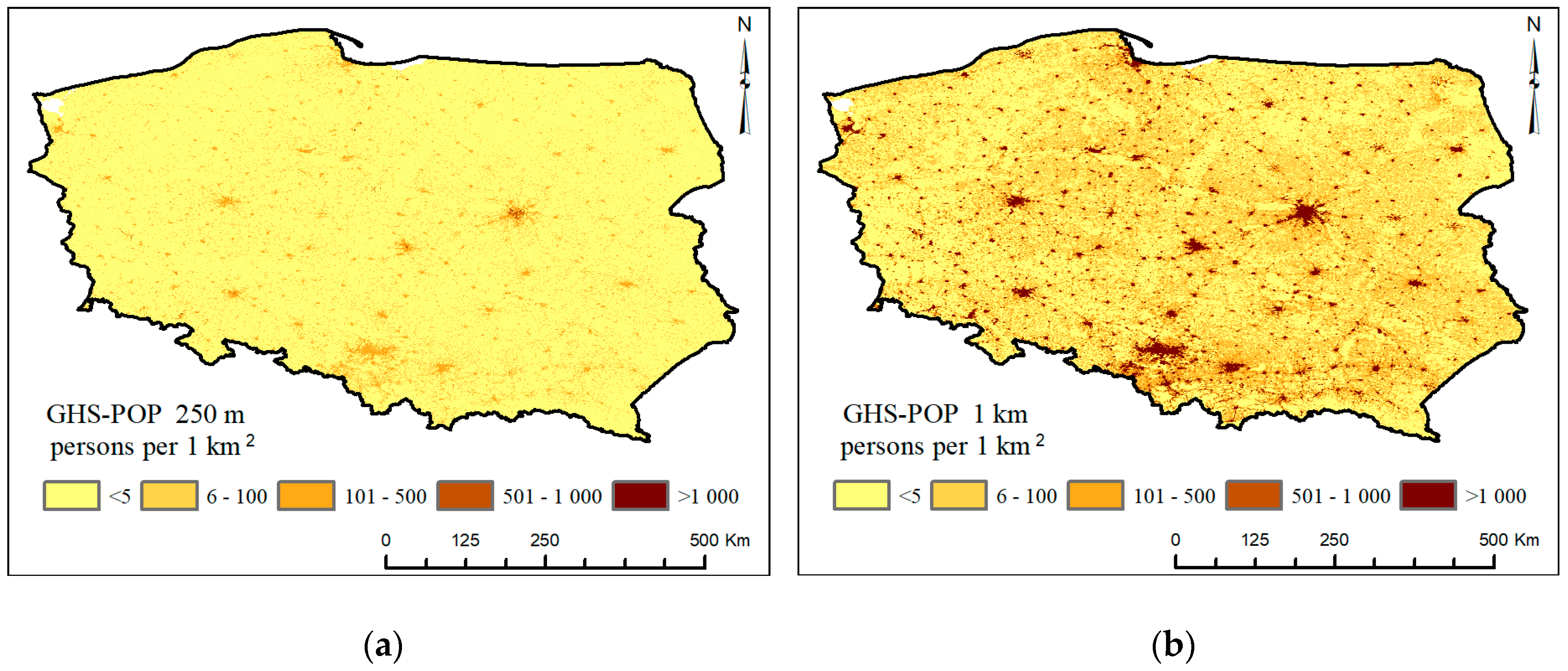
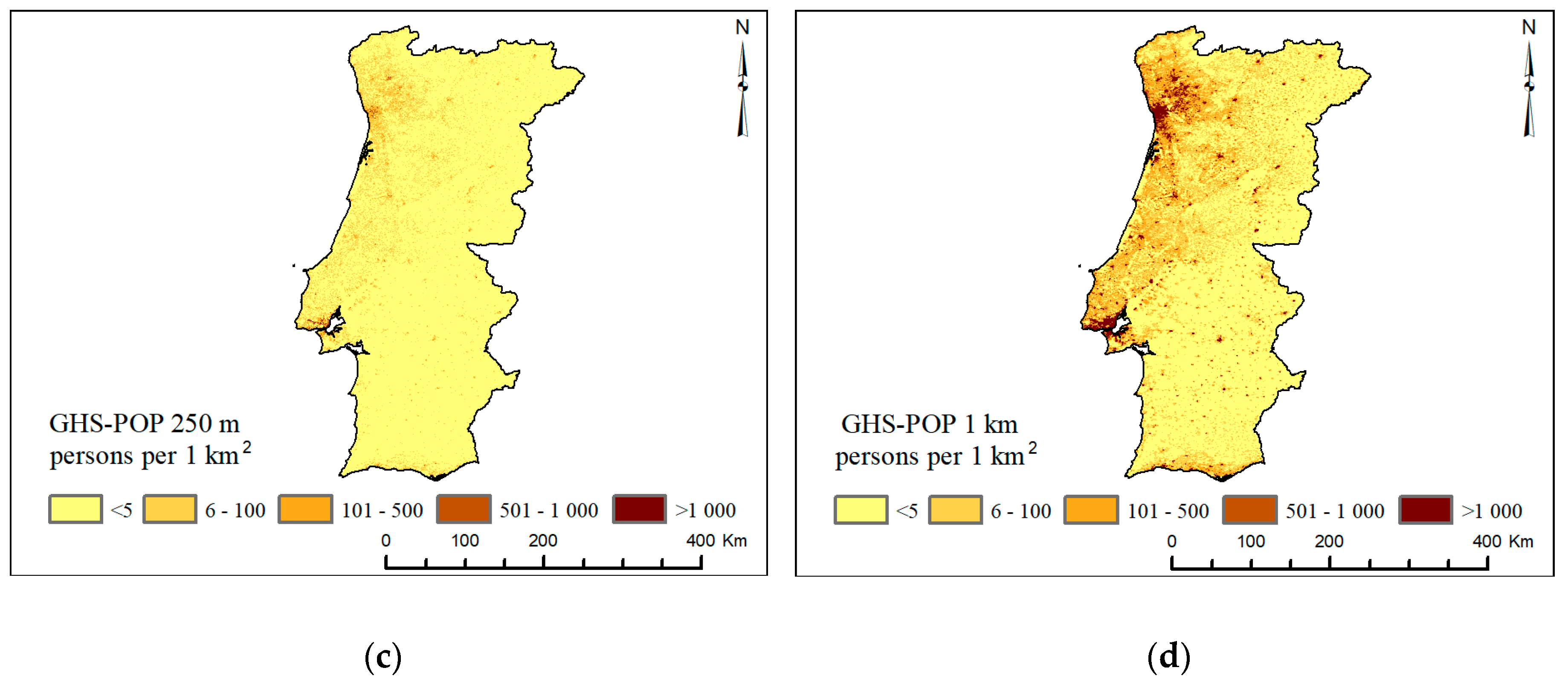
2.2. The GHS-POP Data
2.3. Census Data
3. Methods
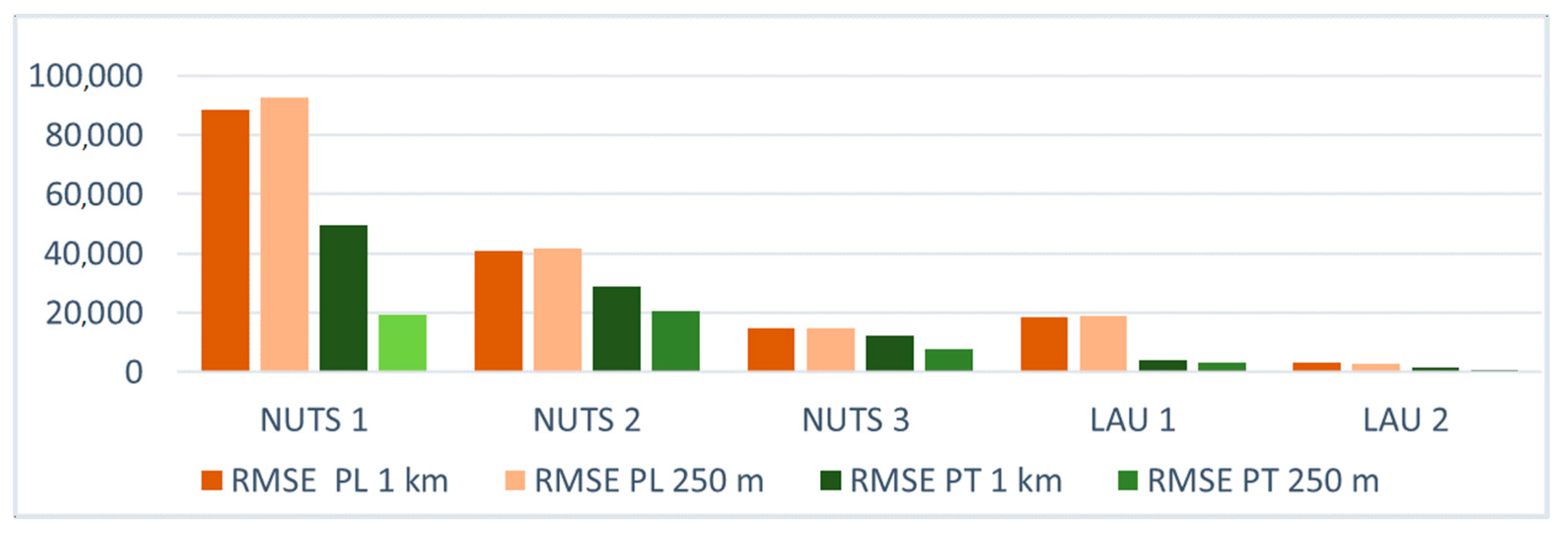
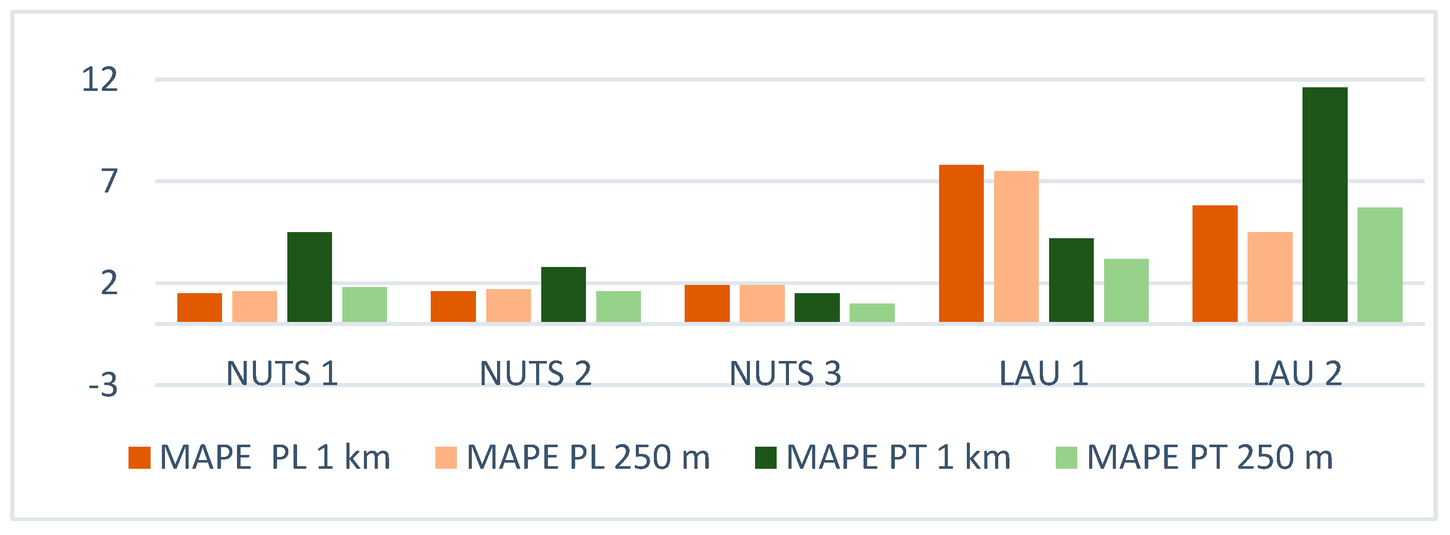
- What is the accuracy of the GHS-POP? Do the results of the data accuracy assessment change depending on the reference unit size? Which administrative level presents the highest errors?The answer to this question is based on the analysis of MAE, RMSE, and MAPE calculated for reference units at six administrative levels (from country to municipality).
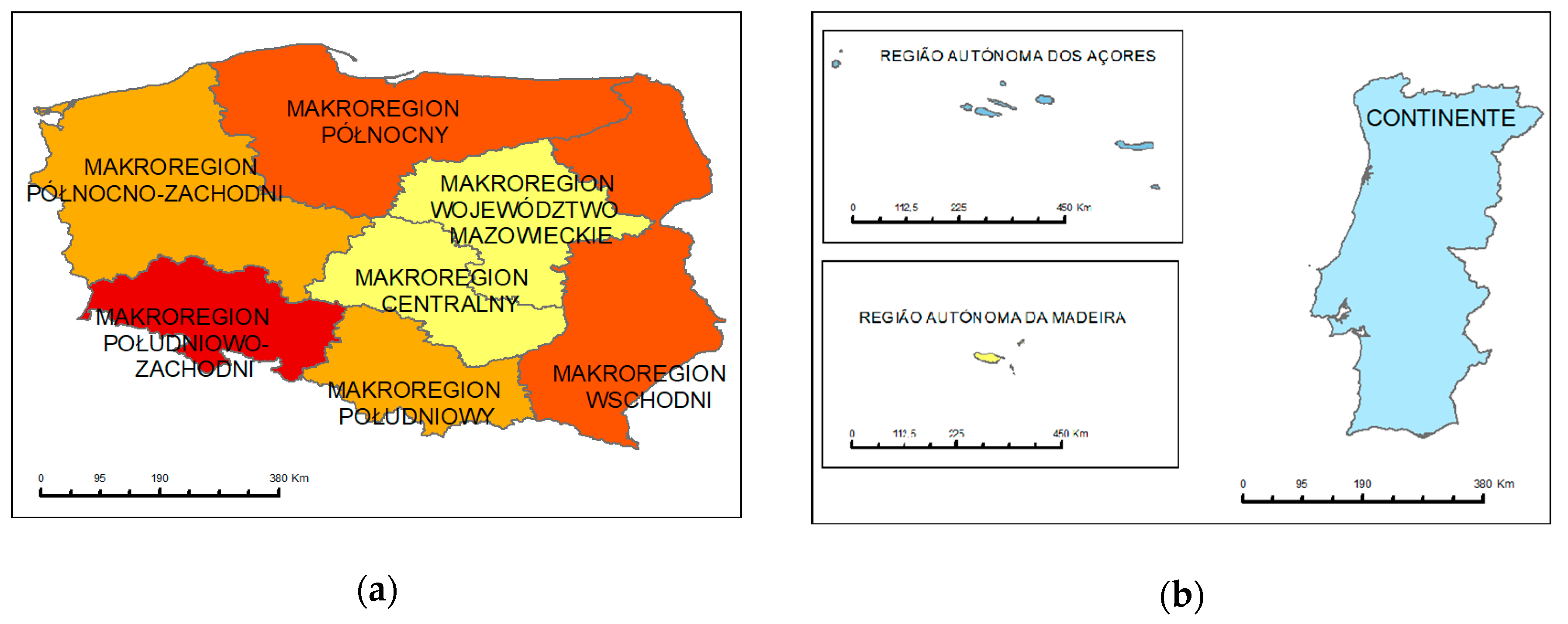
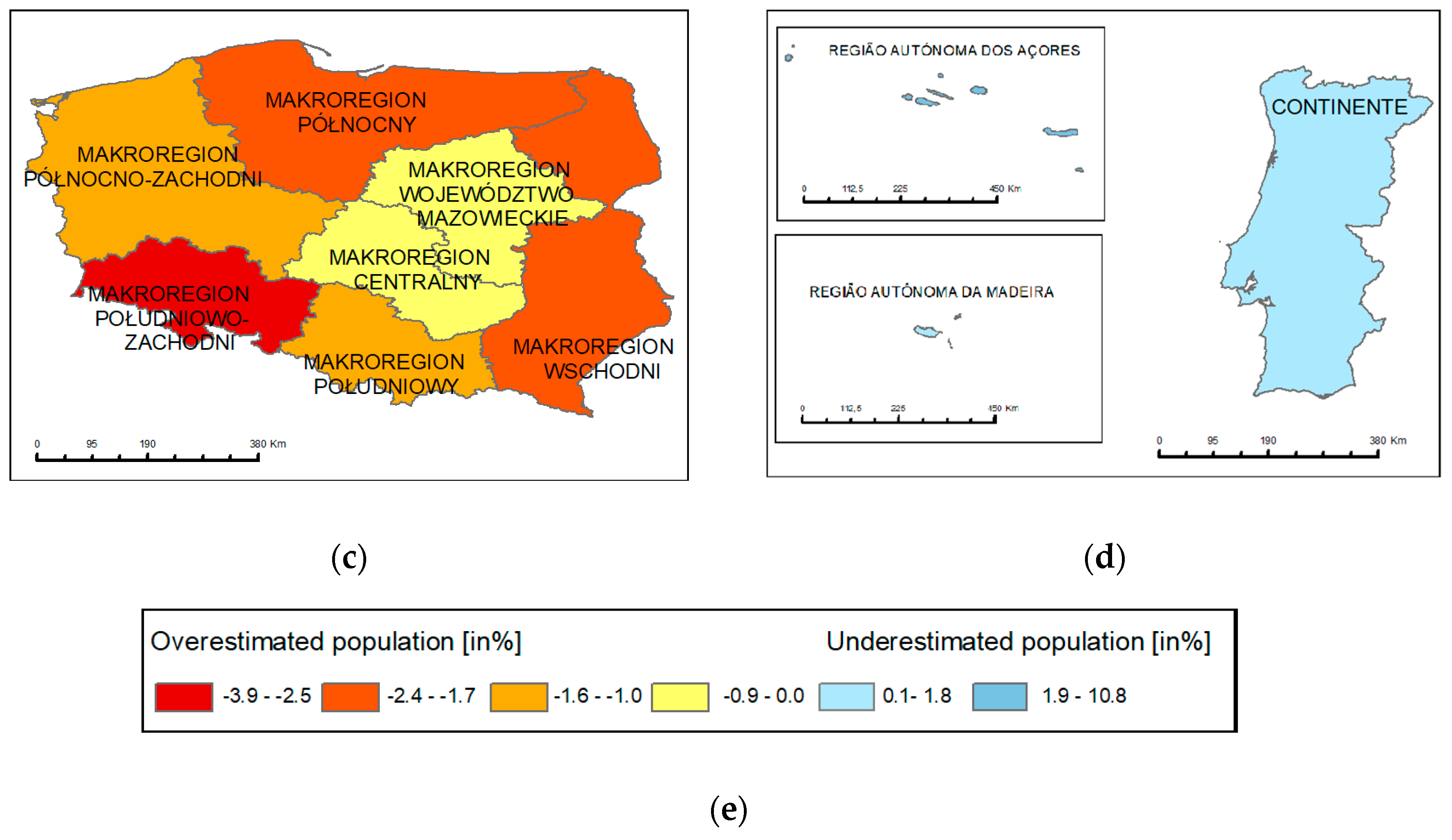
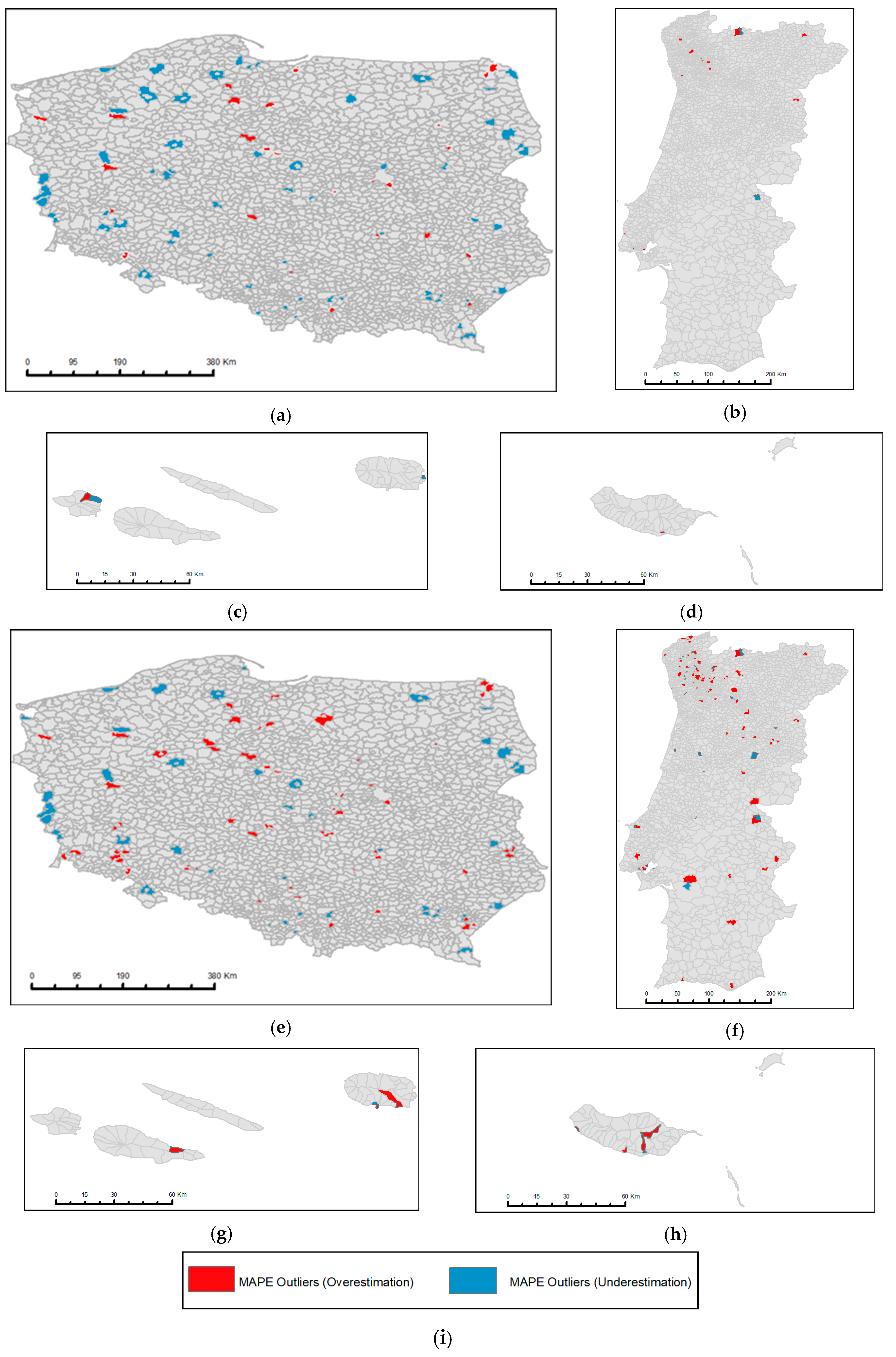
- What are the maximum and minimum MAPE values at each administrative level? Where are the units with maximum underestimation and overestimation located? Are the differences between MAPEs of GHS-POP 1 km and GHS-POP 250 m significant?The values and the spatial diversity of the MAPE for administrative units are shown on the choropleth maps. The answer to this question allows us to discover administrative units with the maximum overestimations and underestimations of the population for GHS-POP 1 km and GHS-POP 250 m. It also allows us to indicate units with the highest differences between MAPE values for 250 m and 1 km grid cells.
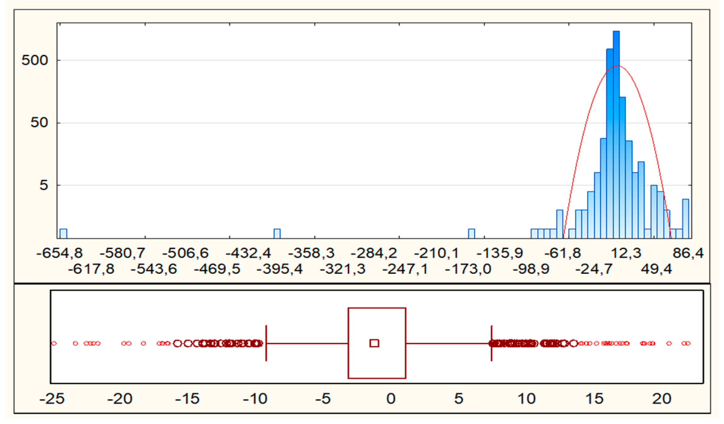
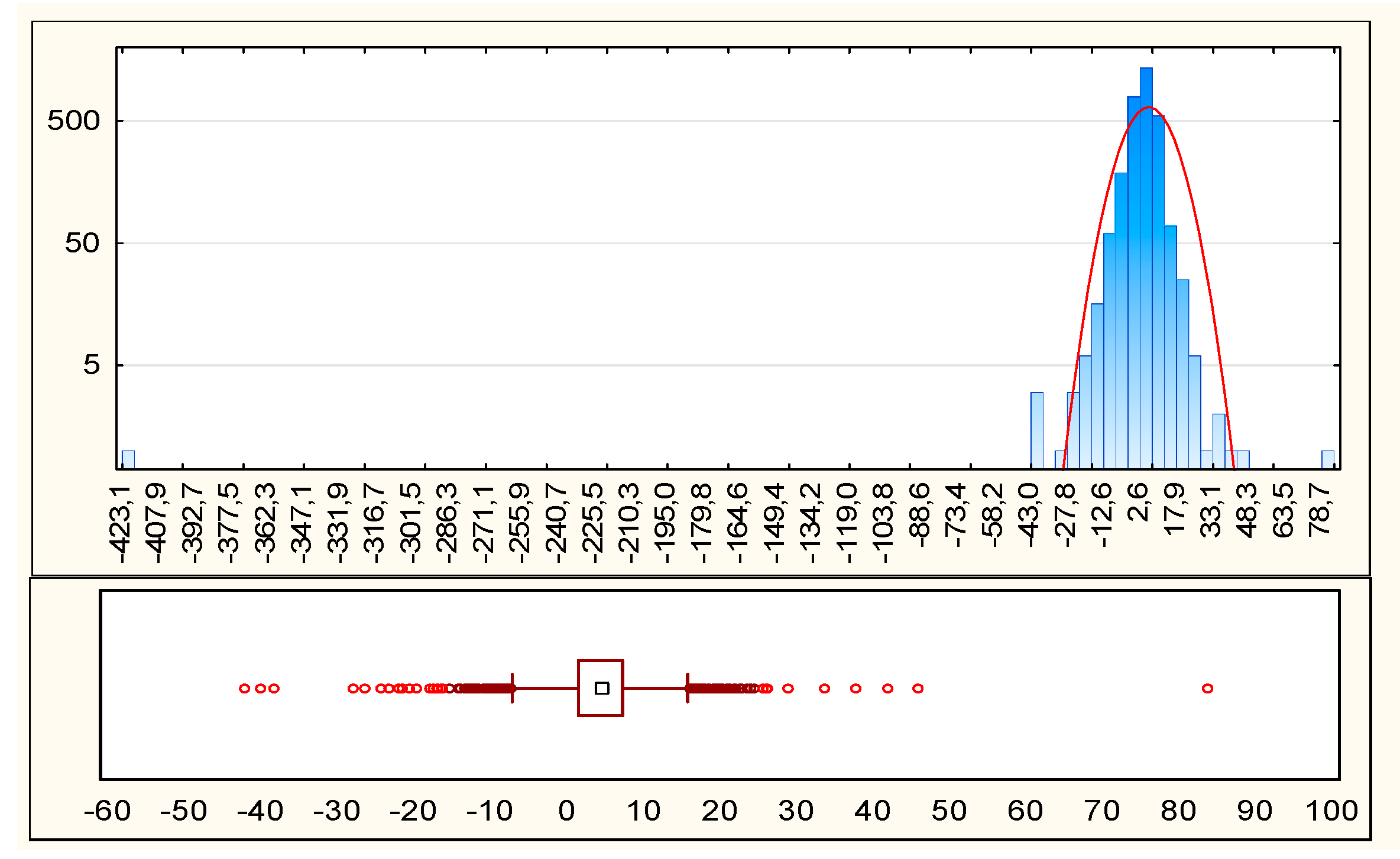
- Is the spatial pattern of the MAPE at LAU 2 really random? What is the MAPE structure and diversity?The answer is based on testing spatial autocorrelation based on administrative unit locations and MAPE values simultaneously. The Moran’s I index value as well as the Z score and p-value were calculated. The diversity of the MAPE was evaluated with use of the statistical measures of central tendency, position, and dispersion (i.e., the mean, median, and the coefficient of variation. The box plot analysis was used to detect extreme MAPE value outliers.
4. Results
4.1. Error Determination
4.2. Cartographic Visualization of MAPE
4.2.1. NUTS 1
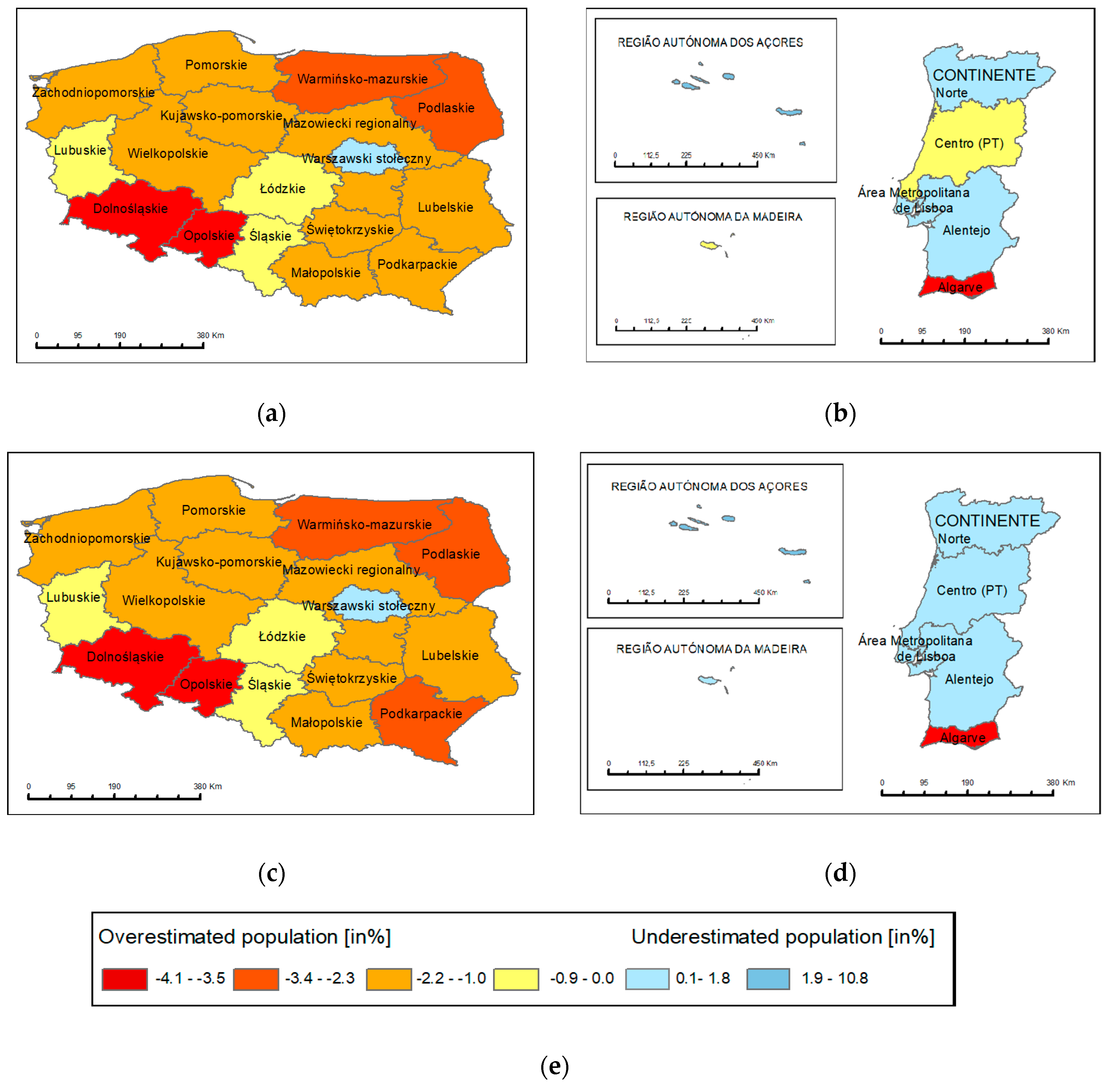
4.2.2. NUTS 2
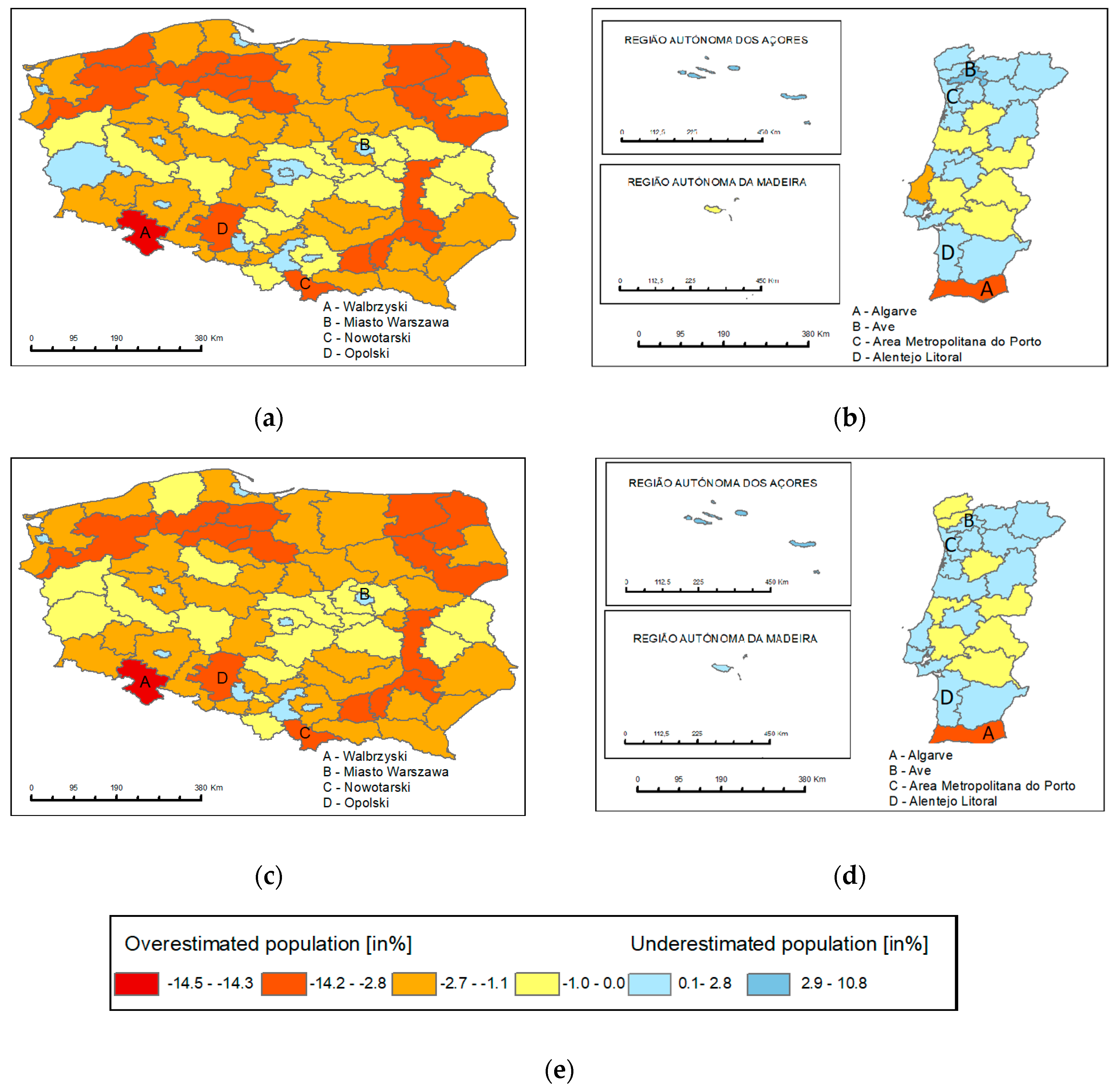
4.2.3. NUTS 3
4.2.4. LAU 1 (NUTS 4)
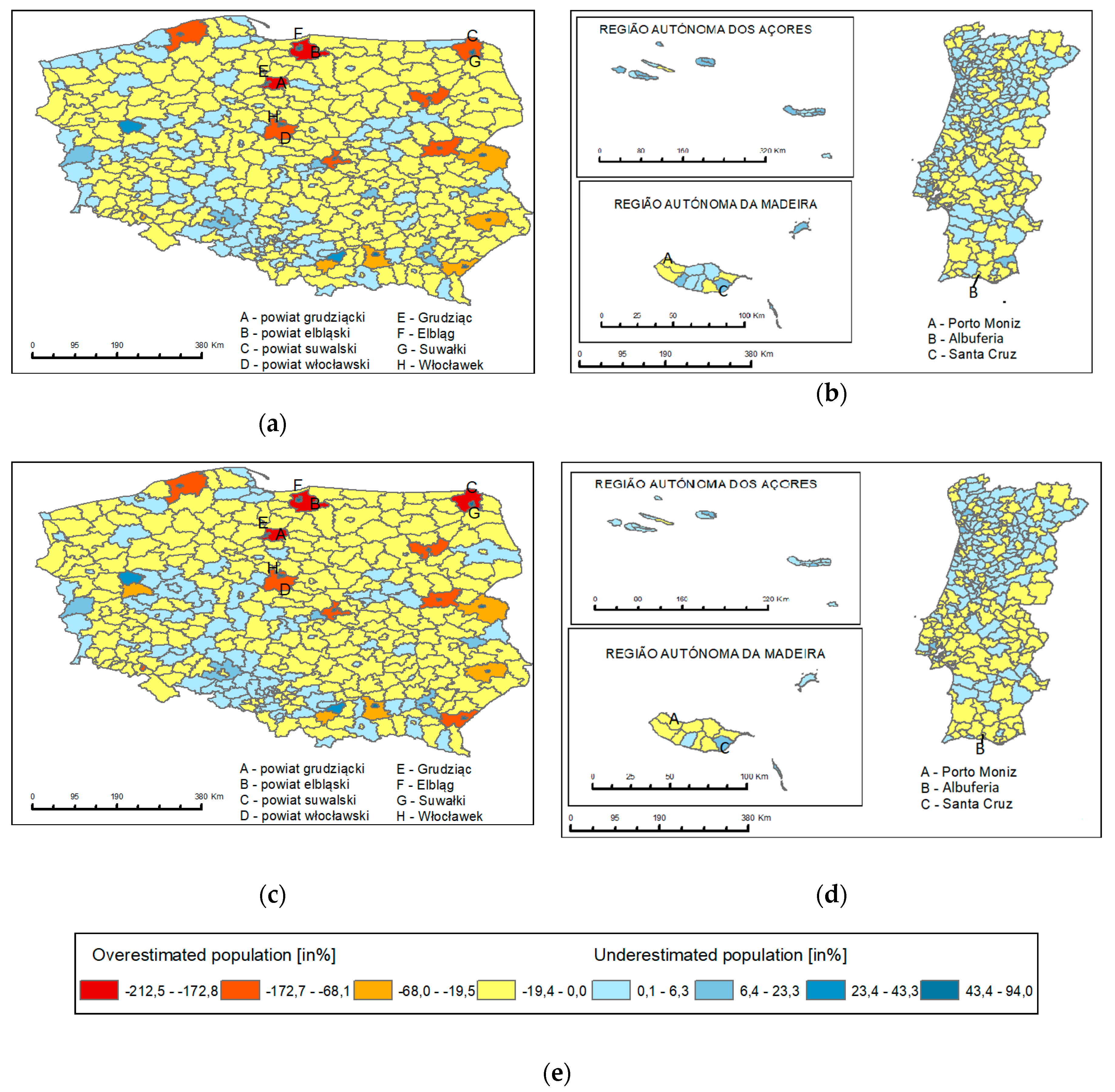
4.2.5. LAU 2 (NUTS 5)
4.3. LAU 2: Spatial Distribution and Statistics of Extreme Outliers
5. Discussion
6. Conclusions
Author Contributions
Funding
Acknowledgments
Conflicts of Interest
References
- Mennis, J.; Hultgren, T. Intelligent dasymetric mapping and its application to areal interpolation. Cartogr. Geogr. Inf. Sci. 2006, 33, 179–194. [Google Scholar] [CrossRef]
- Guo, H.; Cao, K.; Wang, P. Population estimation in Singapore based on remote sensing and open data. In Proceedings of the International Archives of the Photogrammetry, Remote Sensing and Spatial Information Sciences, Wuhan, China, 18–22 September 2017. [Google Scholar]
- Dong, P.; Ramesh, S.; Nepali, A. Evaluation of small-area population estimation using LiDAR, Landsat TM and parcel data. Int. J. Remote Sens. 2010, 31, 5571–5586. [Google Scholar] [CrossRef]
- Douglass, R.W.; Meyer, D.A.; Ram, M.; Rideout, D.; Song, D. High resolution population estimates from telecommunications data. EPJ Data Sci. 2015, 4, 1–13. [Google Scholar] [CrossRef]
- Novack, T.; Kux, H.; Freitas, C. Estimation of Population Density of Census Sectors Using Remote Sensing Data and Spatial Regression. In Geocomputation, Sustainability and Environmental Planning; Studies in Computational Intelligence; Murgante, B., Borruso, G., Lapucci, A., Eds.; Springer: Berlin/Heidelberg, Germany, 2011; Volume 348. [Google Scholar] [CrossRef]
- Wang, L.; Wu, C. Population estimation using remote sensing and GIS technologies. Int. J. Remote Sens. 2010, 31, 5569–5570. [Google Scholar] [CrossRef]
- Wardrop, N.A.; Jochem, W.C.; Bird, T.J.; Chamberlain, H.R.; Clarke, D.; Kerr, D.; Bengtsson, L.; Juran, S.; Seaman, V.; Tatem, A.J. Spatially disaggregated population estimates in the absence of national population and housing census data. Proc. Natl. Acad. Sci. USA 2018, 115, 3529–3537. [Google Scholar] [CrossRef]
- Deng, C.; Wu, C.; Wang, L. Improving the housing-unit method for small-area population estimation using remote-sensing and GIS information. Int. J. Remote Sens. 2010, 31, 5673–5688. [Google Scholar] [CrossRef]
- Wu, S.; Qiu, X.; Wang, L. Population Estimation Methods in GIS and Remote Sensing: A Review. GISci. Remote Sens. 2005, 42, 80–96. [Google Scholar] [CrossRef]
- Pirowski, T.; Bartos, K. Detailed mapping of the distribution of a city population based on information from the national database on buildings. Geod. Vestn. 2018, 62, 458–471. [Google Scholar] [CrossRef]
- Wu, C.; Murray, A.T. Population estimation using Landsat enhanced thematic mapper imagery. Geogr. Anal. 2007, 39, 26–43. [Google Scholar] [CrossRef]
- Lo, C.P. Applied Remote Sensing; Longman: London, UK, 1986. [Google Scholar]
- Tobler, W.R. Satellite confirmation of settlement size coefficients. Area 1969, 1, 30–34. [Google Scholar]
- Lo, C.P.; Welch, R. Chinese urban population estimates. Ann. Assoc. Am. Geogr. 1977, 67, 246–253. [Google Scholar] [CrossRef]
- Stern, M. Landsat data for population estimates -approaches to inter-censal counts in the rural Sudan. In Remote Sensing from Satellites; Carter, W.D., Engman, E.T., Eds.; Pergamon: New York, NY, USA, 1984; pp. 117–125. [Google Scholar]
- Patino, J.E.; Duque, J.C. A review of regional science applications of satellite remote sensing in urban settings. Comput. Environ. Urban. Syst. 2013, 37, 1–17. [Google Scholar] [CrossRef]
- Lo, C.P. Automated population and dwelling unit estimation from highresolution satellite images: A GIS approach. Int. J. Remote Sens. 1995, 16, 17–34. [Google Scholar] [CrossRef]
- Yuan, Y.; Smith, R.M.; Limp, W.F. Remodeling census population with spatial information from Landsat TM imagery. Comput. Environ. Urban. Syst. 1997, 21, 245–258. [Google Scholar] [CrossRef]
- Harvey, J.T. Population estimation models based on individual TM pixels. Photogramm. Eng. Remote Sens. 2002, 68, 1181–1192. [Google Scholar]
- Li, G.; Weng, Q. Using Landsat ETM+ imagery to measure population density in Indianapolis, Indiana, USA. Photogramm. Eng. Remote Sens. 2005, 71, 947–958. [Google Scholar] [CrossRef]
- Liu, D.; Weng, Q.; Li, G. Residential population estimation using remote sensing derived impervious surface. Int. J. Remote Sens. 2006, 27, 3553–3570. [Google Scholar] [CrossRef]
- Galeon, F.A. Estimation of population in informal settlement communities using high resolution satellite image. Int. Arch. Photogramm. Remote Sens. Spat. Inf. Sci. 2008, 37 Pt B4, 1377–1382. [Google Scholar]
- Qiu, F.; Sridharan, H.; Chun, Y. Spatial autoregressive model for population estimation at the census block level using LIDAR-derived building volume information. Cartogr. Geogr. Inf. Sci. 2010, 37, 239–257. [Google Scholar] [CrossRef]
- Ramesh, S. High Resolution Satellite Images and LiDAR Data for Small-Area Building Extraction and Population Estimation. Master’s Thesis, University of North Texas, Denton, TX, USA, 2009. [Google Scholar]
- Weng, Q. Remote sensing of impervious surfaces in the urban areas: Requirements, methods, and trends. Remote Sens. Environ. 2012, 117, 34–49. [Google Scholar] [CrossRef]
- Leyk, S.; Gaughan, A.E.; Adamo, S.B.; de Sherbinin, A.; Balk, D.; Freire, S.; Rose, A.; Stevens, F.R.; Blankespoor, B.; Frye, C.; et al. The spatial allocation of population: A review of large-scale gridded population data products and their fitness for use. Earth Syst. Sci. Data 2019, 11, 1385–1409. [Google Scholar] [CrossRef]
- Balk, D.L.; Deichman, U.; Yetman, G.; Pozzi, F.; Hay, S.I.; Nelson, A. Determining global population distribution: Methods, applications and data. Adv. Parasitol. 2006, 62, 119–156. [Google Scholar] [PubMed]
- CESIN—Center for International Earth Science Information Network Columbia University. Gridded Population of the World, Version 4 (GPWv4): Data Quality Indicators, Beta Release; NASA Socioeconomic Data and Applications Center (SEDAC): Palisades, NY, USA, 2015. [CrossRef]
- Doxsey-Whitfield, E.; MacManus, K.; Adamo, S.B.; Pistolesi, L.; Squires, J.; Borkovska, O.; Baptista, S.R. Taking Advantage of the Improved Availability of Census Data: A First Look at the Gridded Population of the World, Version 4. Appl. Geogr. 2015, 1, 226–234. [Google Scholar] [CrossRef]
- Balk, D.; Yetman, G. The Global Distribution of Population: Evaluating the Gains in Resolution Refinement. Center for International Earth Science Information Network (CIESIN), 2005. Columbia University. Available online: http://beta.sedac.ciesin.columbia.edu/gpw/docs/gpw3_documentation_final.pdf (accessed on 6 June 2019).
- Bellucci, A.; Tholey, N.; Studer, M.; Goester, J.F.; Fuentes, N. Extrapolation of population grids for risk analysis. J. Space Saf. Eng. 2018, 5, 192–196. [Google Scholar] [CrossRef]
- Chu, H.-J.; Yang, C.-H.; Chou, C.C. Adaptive Non-Negative Geographically Weighted Regression for Population Density Estimation Based on Nighttime Light. ISPRS Int. J. Geo-Inf. 2019, 8, 26. [Google Scholar] [CrossRef]
- Calka, B.; Bielecka, E. Reliability Analysis of LandScan Gridded Population Data. The Case Study of Poland. ISPRS Int. J. Geo-Inf. 2019, 8, 222. [Google Scholar] [CrossRef]
- Bhaduri, B.; Bright, E.; Coleman, P. Development of a High Resolution Population Dynamics Model. Paper Presented at Geocomputation 2005, Ann Arbor, Michigan. Available online: http://www.geocomputation.org/2005/Abstracts/Bhaduri.pdf (accessed on 10 June 2019).
- Stevens, F.; Gaughan, A.E.; Linard, C.; Tatem, A.J. Disaggregating Census Data for Population Mapping Using Random Forests with Remotely-Sensed and Ancillary Data. PLoS ONE 2015, 10, e0107042. [Google Scholar] [CrossRef]
- Sabesan, A.; Abercrombie, K.; Ganguly, A.R.; Bhaduri, B.; Bright, E.A.; Coleman, P.R. Metrics for the comparative analysis of geospatial datasets with applications to high-resolution grid-based population data. GeoJournal 2007, 69, 81–91. [Google Scholar] [CrossRef]
- Calka, B.; Nowak Da Costa, J.; Bielecka, E. Fine scale population density data and its application in risk assessment. Geomat. Nat. Hazards Risk 2017, 8, 1440–1455. [Google Scholar] [CrossRef]
- Tatem, A.J.; Gaughan, A.E.; Stevens, F.R.; Patel, N.N.; Jia, P.; Pandey, A.; Linard, C. Quantifying the effects of using detailed spatial demographic data on health metrics: A systematic analysis for the AfriPop, AsiaPop, and AmeriPop projects. Lancet N. Am. Ed. 2013, 381, S142. [Google Scholar] [CrossRef]
- Gaughan, A.E.; Stevens, F.R.; Linard, C.; Jia, P.; Tatem, A.J. High Resolution Population Distribution Maps for Southeast Asia in 2010 and 2015. PLoS ONE 2013, 8, e55882. [Google Scholar] [CrossRef] [PubMed]
- Freire, S.; MacManus, K.; Pesaresi, M.; Doxsey-Whitfield, E.; Mills, J. Development of new open and free multi-temporal global population grids at 250 m resolution. In Proceedings of the 19th AGILE Conference on Geographic Information Science, Helsinki, Finland, 14–17 June 2016. [Google Scholar]
- Pesaresi, M.; Ehrlich, D.; Ferri, S.; Florczyk, A.J.; Freire, S.; Halkia, S.; Julea, A.M.; Kemper, T.; Soille, P.; Syrris, V. Operating Procedure for the Production of the Global Human Settlement Layer from Landsat Data of the Epochs 1975, 1990, 2000, and 2014; EUR 27741 EN; Publications Office of the European Union: Luxembourg, 2016. [CrossRef]
- Bai, Z.; Wang, J.; Wang, M.; Gao, M.; Sun, J. Accuracy Assessment of Multi-Source Gridded Population Distribution Datasets in China. Sustainability 2018, 10, 1363. [Google Scholar] [CrossRef]
- Hay, S.I.; Guerra, C.A.; Tatem, A.J.; Noor, A.M.; Snow, R.W. The global distribution and population at risk of malaria: Past, present, and future. Lancet Infect. Dis. 2004, 4, 327–336. [Google Scholar] [CrossRef]
- Tatem, A.J.; Guerra, C.A.; Kabaria, C.W.; Noor, A.M.; Hay, S.I. Human population, urban settlement patterns and their impact on Plasmodium falciparum malaria endemicity. Malar. J. 2008, 7, 218. [Google Scholar] [CrossRef] [PubMed]
- Uhl, J.H.; Leyk, S. Multi-Scale Effects and Sensitivities in Built-up Land Data accuracy Assessments. Remote Sens Environ. 2018, 204, 898–917. [Google Scholar] [CrossRef]
- Qiao, C.; Sun, R.; Cui, T. Research on scale effect of vegetation net primary productivity. In Proceedings of the 2016 IEEE International Geoscience and Remote Sensing Symposium (IGARSS), Beijing, China, 10–15 July 2016; pp. 1333–1336. [Google Scholar] [CrossRef]
- GUS. Powierzchnia i Ludność w Przekroju Terytorialnym w 2018 Roku; Główny Urząd Statystyczny: Warsaw, Poland, 2012.
- GUS. Ludność w Gminach Według Stanu w Dniu 31.12.2011 r.—Bilans Opracowany w Oparciu o Wyniki NSP 2011; Główny Urząd Statystyczny: Warsaw, Poland, 2012. Available online: https://geo.stat.gov.pl/imap/?locale=en (accessed on 10 June 2019).
- Eurostat. Statistical Yearbook. Available online: https://ec.europa.eu/eurostat/web/ess/portugal/statistics (accessed on 15 June 2019).
- Sleszynski, P. Delimitation of the Functional Urban Areas around Poland’s Voivodship Capital Cities. Przeglad Geograficzny 2013, 85, 173–197. [Google Scholar] [CrossRef]
- Florczyk, A.J.; Corbane, C.; Ehrlich, D.; Freire, S.; Kemper, T.; Maffenini, L.; Melchiorri, M.; Pesaresi, M.; Politis, P.; Schiavina, M.; et al. GHSL Package 2019; EUR 29788EN; JRC117104; Publications Office of the European Union: Luxembourg, 2019; ISBN 978-92-76-08725-0. [CrossRef]
- Corbane, C.; Pesaresi, M.; Politis, P.; Syrris, V.; Florczyk, A.J.; Soille, P.; Maffenini, L.; Burger, A.; Vasilev, V.; Rodriguez, D.; et al. Big earth data analytics on Sentinel-1 and Landsat imagery in support to global human settlements mapping. Big Earth Data 2017, 1, 118–144. [Google Scholar] [CrossRef]
- Eurostat. Population Data. Available online: https://ec.europa.eu/eurostat/web/population-demography-migration-projections/data (accessed on 20 June 2019).
- GUS. Statystyka Regionalna—Regional Statistic. Available online: http://stat.gov.pl/statystyka-regionalna/jednostki-terytorialne/klasyfikacja-nuts/ (accessed on 10 June 2019).
- Tayman, J.; Swanson, D.A. On the validity of MAPE as a measure of population forecast accuracy. Popul. Res. Policy Rev. 1999, 18, 299–322. [Google Scholar] [CrossRef]
- Tayman, J.; Schafer, E.; Carter, L. The role of population size in the determination and prediction of population forecast errors: An evaluation using confidence intervals for subcounty areas. Popul. Res. Policy Rev. 1998, 17, 1–20. [Google Scholar] [CrossRef]
- Waller, L.A.; Gotway, C.A. Applied Spatial Statistics for Public Health Data; John Wiley and Sons: New York, NY, USA, 2004. [Google Scholar]
- Tu, J.; Xia, Z.G. Examining spatially varying relationships between land use and water quality using geographically weighted regression I: Model design and evaluation. Sci. Total Environ. 2008, 407, 358–378. [Google Scholar] [CrossRef]
- Nowak Da Costa, J. Novel Tool to Examine Polygon Features Completeness Based on a Comparative Study of VGI Data and Official Polish Building Datasets. Geodetski Vestnik 2016, 60, 495–508. [Google Scholar] [CrossRef]
- Nowak Da Costa, J.; Bielecka, E.; Calka, B. Jakość danych OpenStreetMap—Analiza informacji o budynkach na terenie Siedlecczyzny. Ann. Geomat. 2016, 14, 193–203. (In Polish) [Google Scholar]
- Stillwell, J.; Thomas, M. How far do internal migrants really move? Demonstrating a new method for the estimation of intra-zonal distance. Reg. Stud. Reg. Sci. 2016, 3, 28–47. [Google Scholar] [CrossRef]
- Martin, R.G. Accuracy assessment of Landsat-based visual change detection methods applied to the rural-urban fringe. Photogramm. Eng. Remote Sens. 1989, 55, 209–215. [Google Scholar]
- Ge, Y.; Jin, Y.; Stein, A.; Chen, Y.; Wang, J.; Wang, J.; Cheng, Q.; Bai, H.; Liu, M.; Atkinson, P.M. Principles and methods of scaling geospatial Earth science data. Earth-Sci. Rev. 2019, 197, 102897. [Google Scholar] [CrossRef]
- Willmott, C.J.; Matsuura, K. Advantages of the mean absolute error (MAE) over the root mean square error (RMSE) in assessing average model performance. Clim. Res. 2005, 30, 79–82. [Google Scholar] [CrossRef]
- Mościcka, A.; Pokonieczny, K.; Wilbik, A.; Wabiński, J. Transport Accessibility of Warsaw: A Case Study. Sustainability 2019, 11, 5536. [Google Scholar] [CrossRef]


| Descriptive Statistics | GHS-POP 250 m Poland | GHS-POP 1 km Poland | GHS-POP 250 m Portugal | GHS-POP 1 km Portugal |
|---|---|---|---|---|
| Number of grid cells | 4,982,749 | 311,647 | 1,423,136 | 88,956 |
| Min. | 0.00 | 0.00 | 0.00 | 0.00 |
| Max. | 3849 | 12,821 | 2668 | 19,414 |
| Median | 0.00 | 6.83 | 0.00 | 0.31 |
| Mean | 7.74 | 123.74 | 6.91 | 109.73 |
| Mode | 0.00 | 0.00 | 0.00 | 0.00 |
| The first quartile (Q1) | 0.00 | 0.00 | 0.00 | 0.00 |
| The third quartile (Q3) | 0.00 | 63.39 | 0.01 | 33.48 |
| Percentile 10 | 0.00 | 0.00 | 0.00 | 0.00 |
| Percentile 90 | 11.37 | 232.11 | 7.28 | 188.25 |
| Standard deviation | 36.46 | 472.29 | 47.21 | 582.09 |
| Skewness | 9.36 | 8.57 | 17.23 | 13.79 |
| Kurtosis | 175.59 | 98.06 | 423.14 | 261.14 |
| Variance | 1329.49 | 223,058.4 | 2229.12 | 338,835.1 |
| Number of people according to Eurostat | 38,005,614 | 10,374,822 | ||
| Poland | Portugal | |
|---|---|---|
| NUTS 0: The area of the whole country | 1 | 1 |
| NUTS 1: Macroregions | 7 | 3 |
| NUTS 2: Regions | 17 | 7 |
| NUTS 3: Groups of counties | 73 | 25 |
| LAU 1 (NUTS 4) | 380 | 308 |
| LAU 2 (NUTS 5) | 2482 | 3092 |
| POLAND | PORTUGAL | |||||||
|---|---|---|---|---|---|---|---|---|
| RMSE | MAE | MAPE (%) | R2 | RMSE | MAE | MAPE (%) | R2 | |
| NUTS 1 | ||||||||
| GHS-POP 1 km | 88,633.42 | 78,233.33 | 1.5% | 0.9990 | 49,696.17 | 37,679.97 | 4.5% | ≈1.000 |
| GHS-POP 250 m | 92,590.10 | 82,353.64 | 1.6% | 0.9990 | 19,480.26 | 14,680.60 | 1.8% | ≈1.000 |
| NUTS 2 | ||||||||
| GHS-POP 1 km | 40,728.07 | 32,494.29 | 1.6% | 0.0993 | 28,911.45 | 20,796.51 | 2.8% | 0.9998 |
| GHS-POP 250 m | 41,717.26 | 34,081.67 | 1.7% | 0.9994 | 20,396.73 | 12,544.67 | 1.6% | 0.9999 |
| NUTS 3 | ||||||||
| GHS-POP 1 km | 14,728.36 | 9392.25 | 1.9% | 0.9711 | 12,461.90 | 6310.94 | 1.5% | 0.9998 |
| GHS-POP 250 m | 14,629.63 | 9240.49 | 1.9% | 0.9726 | 7747.00 | 3993.05 | 1.0% | 0.9999 |
| LAU 1 (NUTS 4) | ||||||||
| GHS-POP 1 km | 18,525.99 | 6296.60 | 7.8% | 0.9753 | 4084.98 | 1354.32 | 4.2% | 0.9967 |
| GHS-POP 250 m | 19,051.75 | 6078.21 | 7.5% | 0.9739 | 3156.08 | 1020.45 | 3.2% | 0.9945 |
| LAU 2 (NUTS 5) | ||||||||
| GHS-POP 1 km | 2945.81 | 733.24 | 5.8% | 0.9716 | 1330.04 | 407.57 | 11.6% | 0.9650 |
| GHS-POP 250 m | 2935.74 | 608.21 | 4.5% | 0.9699 | 465.85 | 163.88 | 5.71% | 0.9958 |
| Descriptive Statistics | Poland 250 m | Poland 1 km | Portugal 250 m | Portugal 1 km |
|---|---|---|---|---|
| Moran’s index | 0.0049 | −0.0019 | 0.0129 | −0.0007 |
| z-score | 0.4870 | −0.1291 | 1.6204 | −0.2483 |
| p-value | 0.6263 | 0.8973 | 0.9760 | 0.8031 |
| Random | Random | Random | Random |
| Descriptive Statistics | MAPE 250 m Poland | MAPE 1 km Poland | MAPE 250 m Portugal | MAPE 1 km Portugal |
|---|---|---|---|---|
| Grubbs Test Statistics | 36.80 p = 0.000 | 35.04 p = 0.000 | 44.40 p = 0.000 | 22.70 p = 0.000 |
| Min. | −654.83 | −660.88 | −423.15 | −423.96 |
| Max. | 86.44 | 82.44 | 83.75 | 98.91 |
| Median | −1.23 | −1.32 | 4.61 | 5.11 |
| Mean | −1.13 | −1.70 | 1.04 | −0.02 |
| Trimmed mean (10%) | −1.18 | −0.52 | 0.63 | −0.01 |
| The first quartile (Q1) | −3.96 | −3.18 | 1.51 | −1.00 |
| The third quartile (Q3) | 1.08 | 1.71 | 7.30 | 9.48 |
| Percentile 10 | −5.14 | −7.70 | −1.91 | −12.70 |
| Percentile 90 | 3.92 | 5.47 | 9.33 | 18.39 |
| Standard deviation | 17.77 | 18.81 | 9.62 | 18.84 |
| Skewness | −24.77 | −21.63 | 28.26 | −4.58 |
| Kurtosis | 842.32 | 694.36 | 1259.49 | 92.32 |
| Variance | 315.69 | 353.83 | 28.98 | 10.72 |
| Quartile Range | 4.25 | 5.67 | 5.79 | 10.48 |
| Range | 741.27 | 743.32 | 506.90 | 522.88 |
| Number of objects | 2478 | 3092 | ||
© 2020 by the authors. Licensee MDPI, Basel, Switzerland. This article is an open access article distributed under the terms and conditions of the Creative Commons Attribution (CC BY) license (http://creativecommons.org/licenses/by/4.0/).
Share and Cite
Calka, B.; Bielecka, E. GHS-POP Accuracy Assessment: Poland and Portugal Case Study. Remote Sens. 2020, 12, 1105. https://doi.org/10.3390/rs12071105
Calka B, Bielecka E. GHS-POP Accuracy Assessment: Poland and Portugal Case Study. Remote Sensing. 2020; 12(7):1105. https://doi.org/10.3390/rs12071105
Chicago/Turabian StyleCalka, Beata, and Elzbieta Bielecka. 2020. "GHS-POP Accuracy Assessment: Poland and Portugal Case Study" Remote Sensing 12, no. 7: 1105. https://doi.org/10.3390/rs12071105
APA StyleCalka, B., & Bielecka, E. (2020). GHS-POP Accuracy Assessment: Poland and Portugal Case Study. Remote Sensing, 12(7), 1105. https://doi.org/10.3390/rs12071105