An Integrative Remote Sensing Application of Stacked Autoencoder for Atmospheric Correction and Cyanobacteria Estimation Using Hyperspectral Imagery


 ,
,  ,
, 
Abstract
1. Introduction
2. Materials and Methods
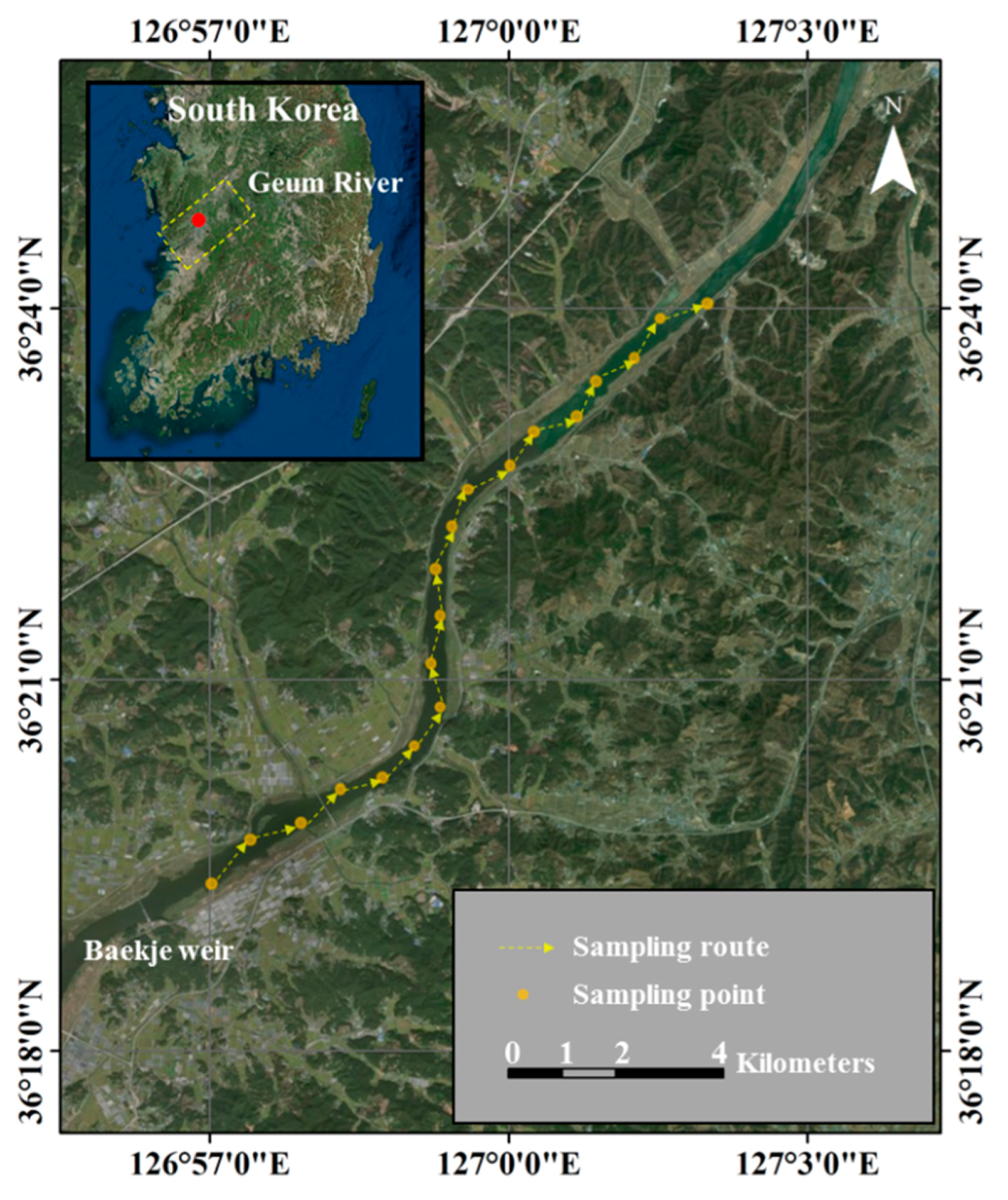
2.1. Study Site
2.2. Dataset
2.2.1. Field and Experimental Data
2.2.2. Hyperspectral Image Sensing
2.3. Data-Driven Models
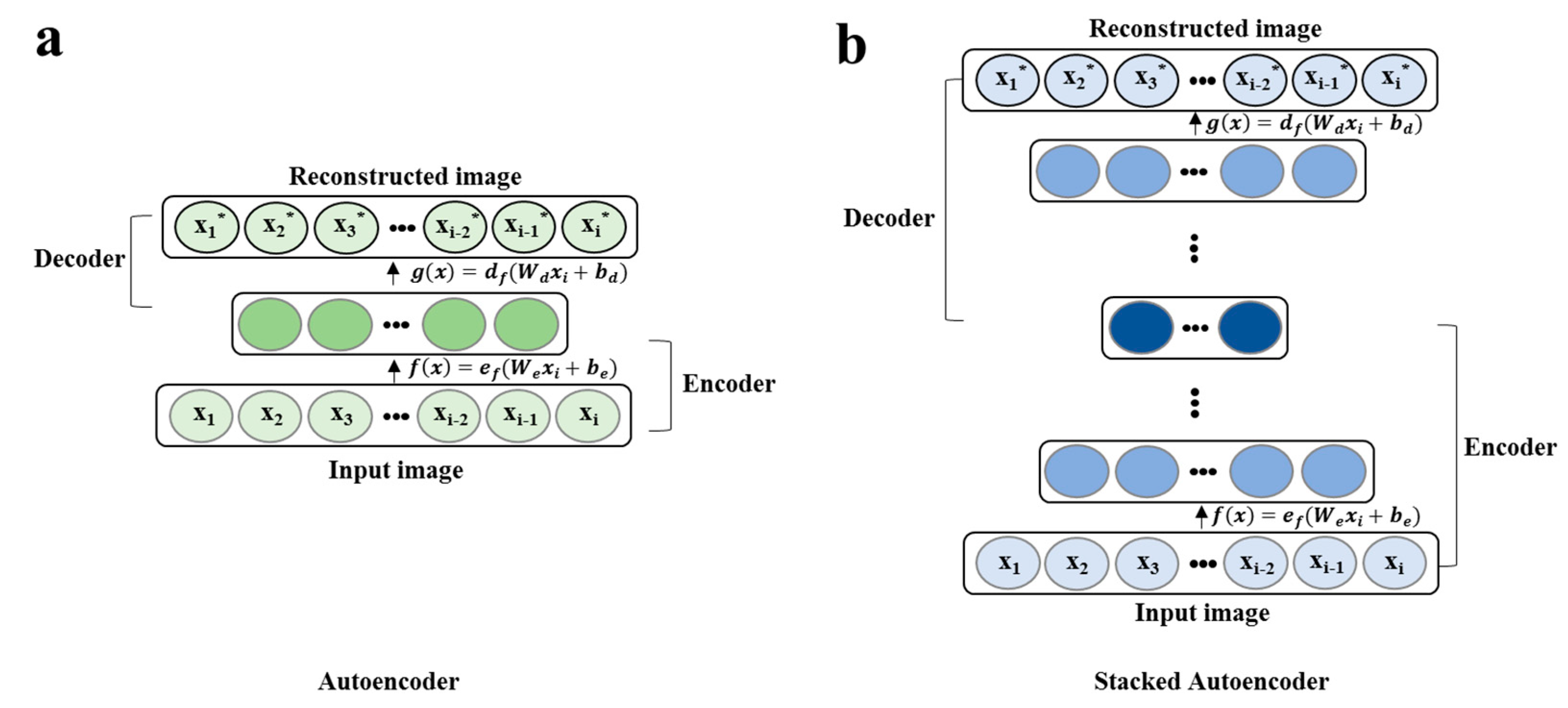
2.3.1. Autoencoder
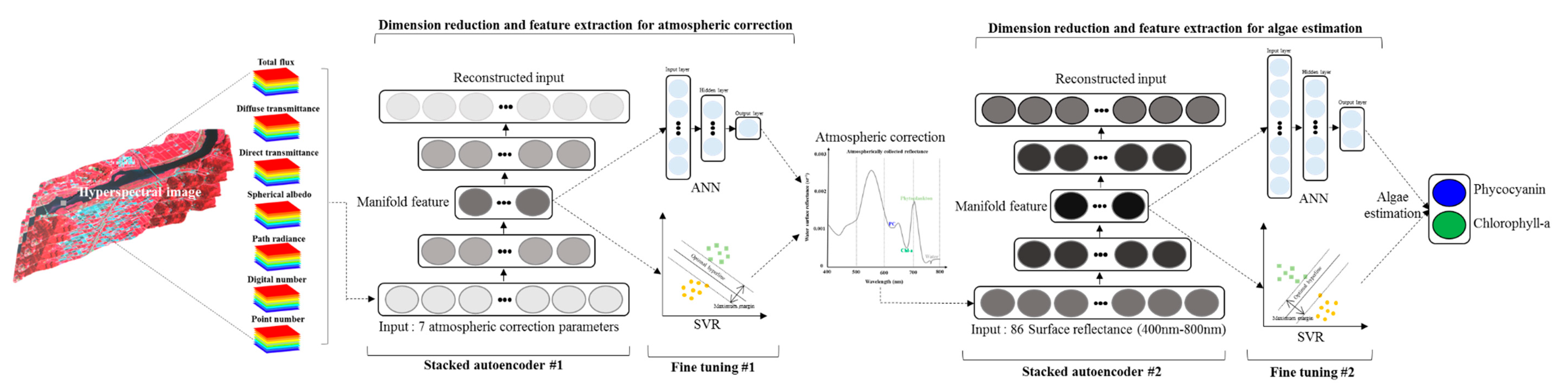
2.3.2. Stacked Autoencoder (SAE)
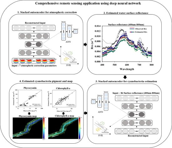
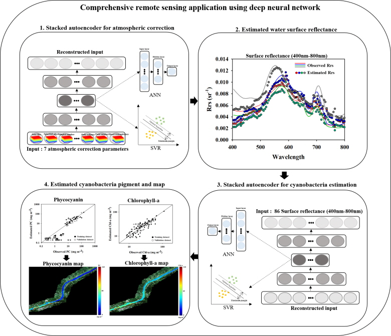
2.3.3. Stacked Autoencoder with ANN and SVR
2.3.4. Model Comparison
2.4. Accuracy
3. Results
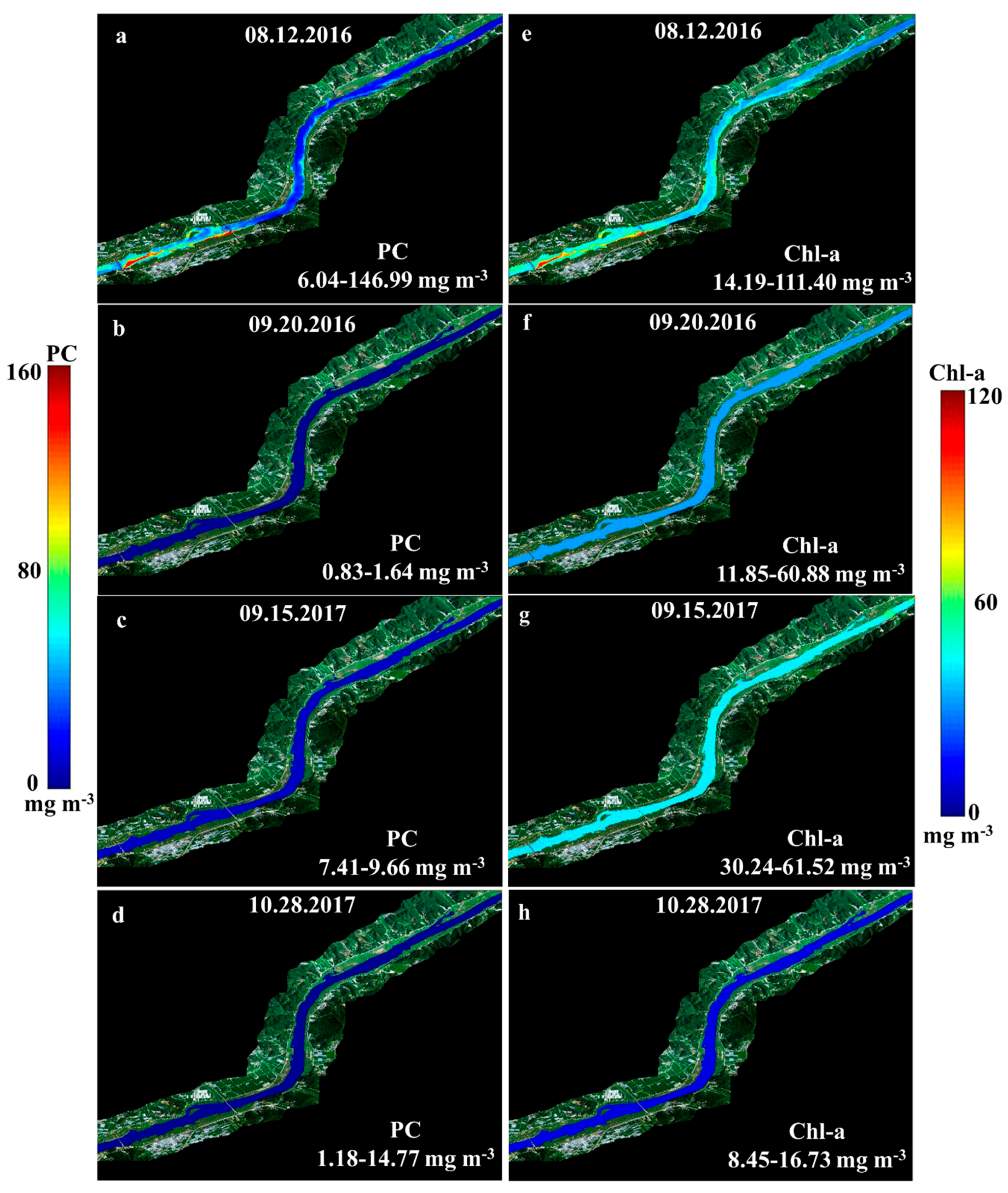
3.1. Variations in Concentrations of the Observed Pigments
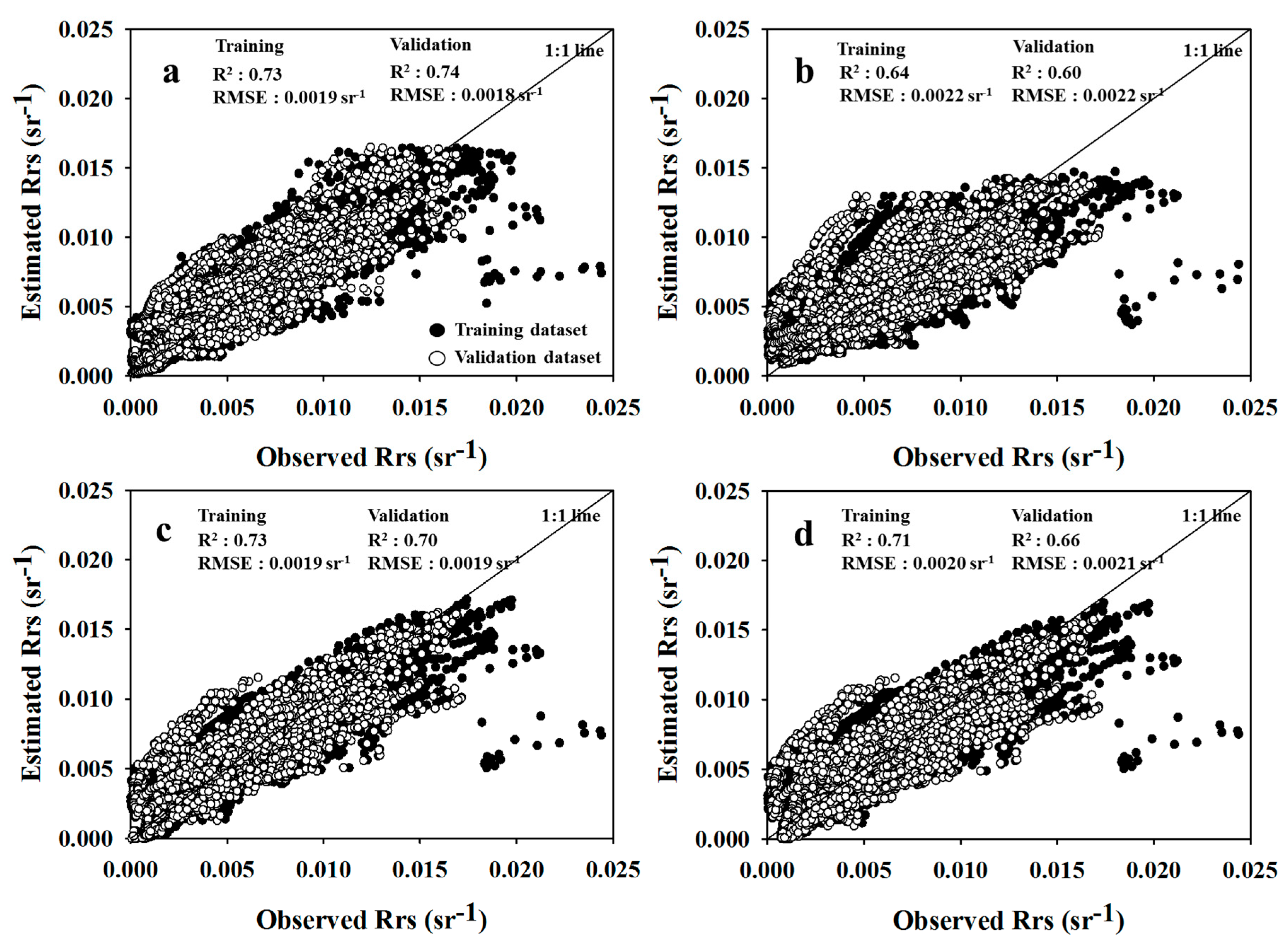
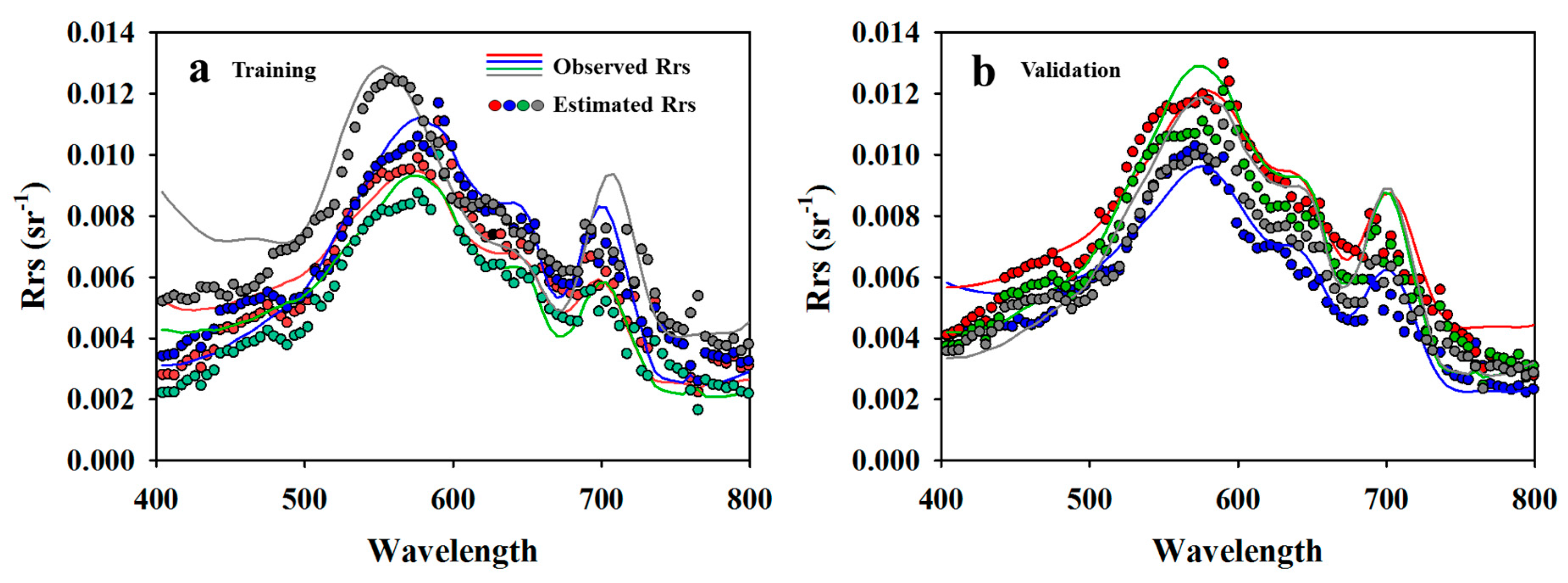
3.2. AC Performance of SAE
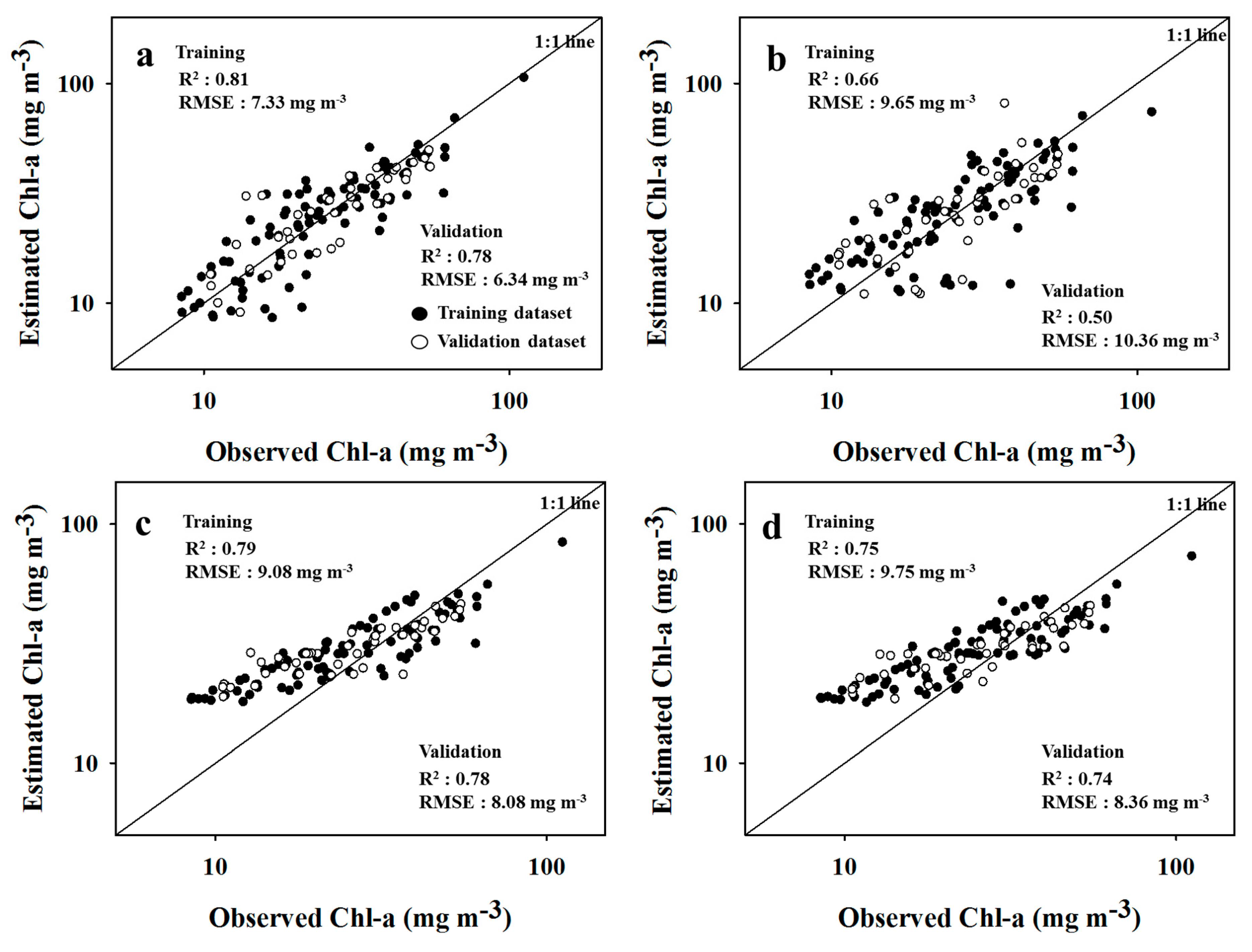
3.3. Cyanobacteria Estimation of SAE
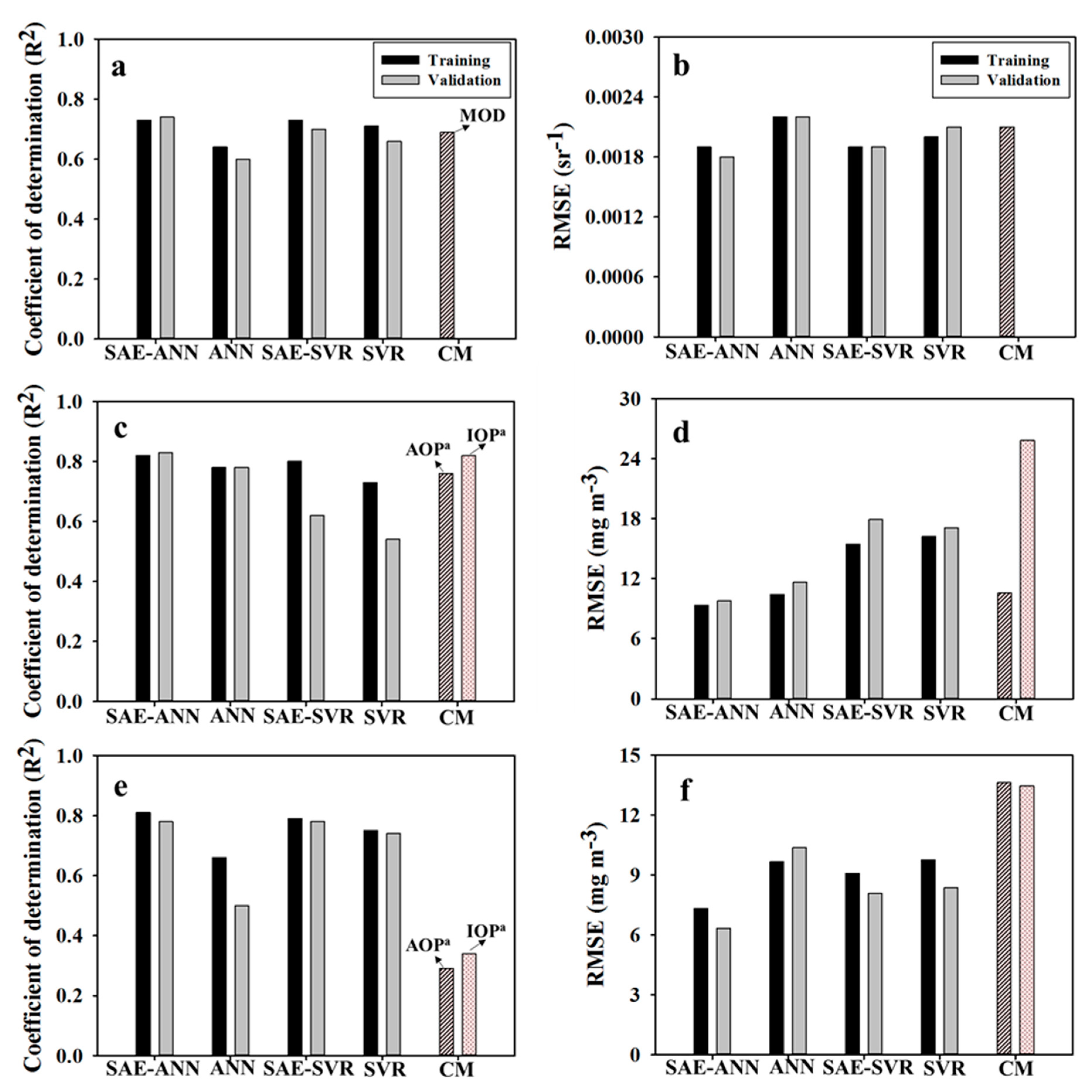
3.4. Model Comparison
4. Discussion
4.1. AC and Cyanobacteria Estimation
4.2. Data-Driven Model Comparison
4.3. Deep Neural Network for Remote Sensing Application
5. Conclusions
- SAE-ANN and -SVR models for AC showed good agreement with the observed reflectance spectra (i.e., NSE > 0.7); the SAE-ANN model estimated the cyanobacteria concentrations with the highest accuracy.
- The encoding layers of the SAE-ANN and -SVR models were able to contribute to the generation of cyanobacterial distribution maps, that represented actual cyanobacterial distribution, by reflecting the varied spatial and spectral features of the input data.
- The SAE-ANN and -SVR models showed an improved accuracy of 23% and 6% for surface reflectance, and 26% and 9% for cyanobacteria estimation, respectively, due to the high-level feature extraction of SAE, compared to the single model performances of ANN and SVR.
Supplementary Materials
Author Contributions
Funding
Acknowledgments
Conflicts of Interest
References
- Hudnell, H.K. The state of U.S. freshwater harmful algal blooms assessments, policy, and legislations. Toxicon 2008, 55, 1024–1034. [Google Scholar] [CrossRef] [PubMed]
- Lee, T.A.; Rollwagen-Bollens, G.; Bollens, S.M.; Faber-Hammond, J.J. Environmental influence on cyanobacteria abundance and microcystin toxin production in a shallow temperate lake. Ecotoxicol. Environ. Saf. 2015, 114, 318–325. [Google Scholar] [CrossRef] [PubMed]
- Cho, K.H.; Kang, J.H.; Ki, S.J.; Park, Y.; Cha, S.M.; Kim, J.H. Determination of the optimal parameters in regression models for the prediction of chlorophyll-a: A case study of the Yeongsan Reservoir, Korea. Sci. Total Environ. 2009, 407, 2536–2545. [Google Scholar] [CrossRef]
- Heisler, J.; Gilbert, P.M.; Burkholder, J.M.; Anderson, D.M.; Cochlan, W.; Dennison, W.C.; Dortch, Q.; Gobler, C.J.; Heil, C.A.; Humphries, E.; et al. Eutrophication and harmful algal blooms: A scientific consensus. Harmful Algae 2008, 8, 3–13. [Google Scholar] [CrossRef]
- Paerl, H.W.; Hall, N.S.; Calandrino, E.S. Controlling harmful cyanobacterial blooms in a world experiencing anthropogenic and climatic-induced change. Sci. Total Environ. 2011, 409, 1739–1745. [Google Scholar] [CrossRef]
- O’neil, J.M.; Davis, T.W.; Burford, M.A.; Gobler, C.J. The rise of harmful cyanobacteria blooms: The potential roles of eutrophication and climate change. Harmful Algae 2012, 14, 313–334. [Google Scholar] [CrossRef]
- Rigosi, A.; Carey, C.C.; Ibelings, B.W.; Brookes, J.D. The interaction between climate warming and eutrophication to promote cyanobacteria is dependent on trophic state and varies among taxa. Limnol. Oceanogr. 2014, 59, 99–114. [Google Scholar] [CrossRef]
- Lehtimaki, J.; Moisander, P.; Sivonen, K.; Kononen, K. Growth, nitrogen fixation, and nodularin production by two baltic sea cyanobacteria. Appl. Environ. Microbiol. 1997, 63, 1647–1656. [Google Scholar] [CrossRef]
- Stewart, W.D.P.; Alexander, G. Phosphorus availability and nitrogenase activity in aquatic blue-green algae. Freshw. Biol. 1971, 1, 389–404. [Google Scholar] [CrossRef]
- Wasmund, N. Occurrence of cyanobacterial blooms in the Baltic Sea in relation to environmental conditions. Int. Rev. Ges. Hydrobiol. Hydrogr. 1997, 82, 169–184. [Google Scholar] [CrossRef]
- Kutser, T.; Metsamaa, L.; Strombeck, N.; Vahtmae, E. Monitoring cyanobacterial blooms by satellite remote sensing. Estuarine Coast. Shelf Sci. 2006, 67, 303–312. [Google Scholar] [CrossRef]
- Randolph, K.; Wilson, J.; Tedesco, L.; Li, L.; Pascual, D.L.; Soyeux, E. Hyperspectral remote sensing of cyanobacteria in turbid productive water using optically active pigments, chlorophyll a and phycocyanin. Remote Sens. Environ. 2008, 112, 4009–4019. [Google Scholar] [CrossRef]
- Agha, R.; Cirés, S.; Wörmer, L.; Domínguez, J.A.; Quesada, A. Multi-scale strategies for the monitoring of freshwater cyanobacteria: Reducing the sources of uncertainty. Water Res. 2012, 46, 3043–3053. [Google Scholar] [CrossRef]
- Simis, S.G.H.; Peter, S.W.M.; Gons, H.J. Remote sensing of the cyanobacterial pigment phycocyanin in turbid inland water. Limnol. Oceanogr. 2005, 50, 237–245. [Google Scholar] [CrossRef]
- Kudela, R.M.; Palacios, S.L.; Austerberry, D.C.; Accorsi, E.K.; Guild, L.S.; Torres-Perez, J. Application of hyperspectral remote sensing to cyanobacterial blooms in inland waters. Remote Sens. Environ. 2015, 167, 196–205. [Google Scholar] [CrossRef]
- Jupp, D.L.; Kirk, J.T.; Harris, G.P. Detection, identification and mapping of cyanobacteria—Using remote sensing to measure the optical quality of turbid inland waters. Mar. Freshw. Res. 1994, 45, 801–828. [Google Scholar] [CrossRef]
- Kutser, T. Quantitative detection of chlorophyll in cyanobacterial blooms by satellite remote sensing. Limnol. Oceanogr. 2004, 49, 2179–2189. [Google Scholar] [CrossRef]
- Kallio, K.; Kutser, T.; Hannonen, T.; Koponen, S.; Pulliainen, J.; Vepsäläinen, J.; Pyhälahti, T. Retrieval of water quality from airborne imaging spectrometry of various lake types in different seasons. Sci. Total Environ. 2001, 268, 59–77. [Google Scholar] [CrossRef]
- Shi, S.; Xu, G. Novel performance prediction model of a biofilm system treating domestic wastewater based on stacked denoising auto-encoder deep learning network. Chem. Eng. J. 2018, 347, 280–290. [Google Scholar] [CrossRef]
- Adler-Golden, S.M.; Matthew, M.W.; Bernstein, L.S.; Levine, R.Y.; Berk, A.; Richtsmeier, S.C.; Acharya, P.K.; Anderson, G.P.; Felde, J.W.; Gardner, J. Atmospheric Correction for Shortwave Spectral Imagery Based on Modtran4. In Imaging Spectrometry V International Society for Optics and Photonics; SPIE: Bellingham, WA, USA, 1999; pp. 61–70. [Google Scholar]
- Bernstein, L.S.; Adler-Golden, S.M.; Sundberg, R.L.; Levine, R.Y.; Perkins, T.C.; Berk, A.; Ratkowski, A.J.; Felde, G.; Hoke, M.L. Validation of the Quick Atmospheric Correction Algorithm for Vnir-Swir Multi-and Hyperspectral Imagery. In Algorithms and Technologies for Multispectral, Hyperspectral, and Ultraspectral Imagery XI International Society for Optics and Photonics; SPIE: Bellingham, WA, USA, 2005; pp. 668–679. [Google Scholar]
- Gao, B.C.; Montes, M.J.; Davis, C.O.; Goetz, A.F. Atmospheric correction algorithms for hyperspectral remote sensing data of land and ocean. Remote Sens. Environ. 2009, 113, S17–S24. [Google Scholar] [CrossRef]
- Hunter, P.D.; Tyler, A.N.; Carvalho, L.; Codd, G.A.; Maberly, S.C. Hyperspectral remote sensing of cyanobacterial pigments as indicators for cell populations and toxins in eutrophic lakes. Remote Sens. Environ. 2010, 114, 2705–2718. [Google Scholar] [CrossRef]
- Van Laake, P.E.; Sanchez-Azofeifa, G.A. Simplified atmospheric radiative transfer modelling for estimating incident PAR using MODIS atmosphere products. Remote Sens. Environ. 2004, 91, 98–113. [Google Scholar] [CrossRef]
- Allali, K.; Bricaud, A.; Claustre, H. Spatial variations in the chlorophyll-specific absorption coefficient of phytoplankton and photosynthetically active pigments in the equatorial Pacific. J. Geophys. Res. 1997, 102, 12413–12423. [Google Scholar] [CrossRef]
- Kimes, D.S.; Knyazikhin, Y.; Privette, J.L.; Abuelgasim, A.A.; Gao, F. Inversion methods for physically-based models. Remote Sens. Rev. 2000, 18, 381–439. [Google Scholar] [CrossRef]
- Le, C.F.; Li, Y.M.; Zha, Y.; Sun, D.; Yin, B. Validation of a Quasi-Analytical Algorithm for highly turbid eutrophic water of Meiliang May in Taihu Lake, China. IEEE Trans. Geosci. Remote Sens. 2009, 47, 2492–2500. [Google Scholar]
- Odermatt, D.; Gitelson, A.; Brando, V.E.; Schaepman, M. Review of constituent retrieval in optically deep and complex waters from satellite imagery. Remote Sens. Environ. 2012, 118, 116–126. [Google Scholar] [CrossRef]
- Camps-Valls, G.; Bruzzone, L.; Rojo-Alvarez, J.L.; Melgani, F. Robust support vector regression for biophysical variable estimation from remotely sensed images. IEEE Geosci. Remote Sens. Lett. 2006, 3, 339–343. [Google Scholar] [CrossRef]
- Kwon, Y.S.; Eunna, J.; Im, J.; Baek, S.H.; Park, Y.E.; Cho, K.H. Developing data-driven models for quantifying Cochlodinium polykrikoides in coastal water. Int. J. Remote Sens. 2018, 39, 68–83. [Google Scholar] [CrossRef]
- Schroeder, T.; Behnert, I.; Schaale, M.; Fischer, J.; Doerffer, R. Atmospheric correction algorithm for MERIS above case-2 waters. Int. J. Remote Sens. 2007, 28, 1469–1486. [Google Scholar] [CrossRef]
- Doerffer, R.; Schiller, H. The MERIS Case 2 water algorithm. Int. J. Remote Sens. 2007, 28, 517–535. [Google Scholar] [CrossRef]
- Park, Y.; Pyo, J.; Kwon, Y.S.; Cha, Y.; Lee, H.; Kang, T.; Cho, K.H. Evaluating physico-chemical influences on cyanobacterial blooms using hyperspectral images in inland water, Korea. Water Res. 2017, 126, 319–328. [Google Scholar] [CrossRef] [PubMed]
- Liu, F.; Xu, F.; Yang, S. A Flood Forecasting Model Based on Deep Learning Algorithms Via Integrating Stacked Autoencoders with BP Neural Network. In Proceedings of the 2017 IEEE Third International Conference on Multimedia Big Data (BigMM), Laguna Hills, CA, USA, 19–21 April 2017; pp. 58–61. [Google Scholar]
- Liu, L.; Chen, R.C. A novel passenger flow prediction model using deep learning methods. Transp. Res. Part C Emerg. Technol. 2017, 84, 74–91. [Google Scholar] [CrossRef]
- Kim, D.M.; Park, H.S.; Chung, S.W. Relationship of the thermal stratification and critical flow velocity near the Baekje Weir in Geum River. J. Korean Soc. Water Environ. 2017, 33, 449–459. [Google Scholar]
- Mobley, C.D. Estimation of the remote-sensing reflectance from above-surface measurements. Appl. Opt. 1999, 38, 7442–7455. [Google Scholar] [CrossRef] [PubMed]
- Zhang, Y.; Liu, M.; Qin, B.; Van Der Woerd, H.J.; Li, J.; Li, Y. Modeling remote-sensing reflectance and retrieving chlorophyll-a concentration in extremely turbid case-2 waters (Lake Taihu, China). IEEE Trans. Geosci. Remote Sens. 2009, 47, 1937–1948. [Google Scholar] [CrossRef]
- Boyer, J.N.; Kelble, C.R.; Ortner, P.B.; & Rudnick, D.T. Phytoplankton bloom status: Chlorophyll a biomass as an indicator of water quality condition in the southern estuaries of Florida, USA. Ecol. Indic. 2009, 9, S56–S67. [Google Scholar] [CrossRef]
- APHA (American Public Health Association). Standard Methods for the Examination of Water and Waste Water, 21st ed.; APHA-AWWA-WPCF: Washington, DC, USA, 2001. [Google Scholar]
- Bennett, A.; Bogorad, L. Complementary chromatic adaptation in a filamentous blue-green alga. J. Cell Biol. 1973, 58, 419–435. [Google Scholar] [CrossRef] [PubMed]
- Berk, A.; Conforti, P.; Kennett, R.; Perkins, T.; Hawes, F.; van den Bosch, J. Modtran® 6: A Major Upgrade of the Modtran® Radiative Transfer Code. In Proceedings of the Hyperspectral Image and Signal Processing: Evolution in Remote Sensing (WHISPERS), 6th Workshop on, Lausanne, Switzerland, 24–27 June 2014; pp. 1–4. [Google Scholar]
- Pyo, J.; Ligaray, M.; Kwon, Y.; Ahn, M.H.; Kim, K.; Lee, H.; Kang, T.; Cho, S.B.; Park, Y.; Cho, K. High-spatial resolution monitoring of phycocyanin and chlorophyll-a using airborne hyperspectral imagery. Remote Sens. 2018, 10, 1180. [Google Scholar] [CrossRef]
- Hinton, G.E.; Salakhutdinov, R.R. Reducing the dimensionality of data with neural networks. Science 2006, 313, 504–507. [Google Scholar] [CrossRef] [PubMed]
- Zabalza, J.; Ren, J.; Zheng, J.; Zheng, J.; Zhao, H.; Qing, C.; Yang, Z.; Du, P.; Marshall, S. Novel segmented stacked autoencoder for effective dimensionality reduction and feature extraction in hyperspectral imaging. Neurocomputing 2016, 185, 1–10. [Google Scholar] [CrossRef]
- Chan, P.P.K.; Lin, Z.; Hu, X.; Eric, C.C.; Yeung, D.S. Sensitivity based robust learning for stacked autoencoder against evasion attack. Neurocomputing 2017, 267, 572–580. [Google Scholar] [CrossRef]
- Cho, K.H.; Sthiannopkao, S.; Pachepsky, Y.A.; Kim, K.W.; Kim, J.H. Prediction of contamination potential of groundwater arsenic in Cambodia, Laos, and Thailand using artificial neural network. Water Res. 2011, 45, 5535–5544. [Google Scholar] [CrossRef] [PubMed]
- Park, Y.; Ligaray, M.; Kim, Y.M.; Kim, J.H.; Cho, K.H.; Sthiannopkao, S. Development of enhanced groundwater arsenic prediction model using machine learning approaches in Southeast Asian countries. Desalination Water Treat. 2016, 57, 12227–12236. [Google Scholar] [CrossRef]
- Du, C.; Wang, Q.; Li, Y.; Lyu, H.; Zhu, L.; Zheng, Z.; Wen, S.; Liu, G.; Guo, Y. Estimation of total phosphorus concentration using a water classification method in inland water. Int. J. Appl. Earth Obs. Geoinf. 2018, 71, 29–42. [Google Scholar] [CrossRef]
- Gonzalez, P.A.; Zamarreno, J.M. Prediction of hourly energy consumption in buildings based on a feedback artificial neural network. Energy Build. 2005, 37, 595–601. [Google Scholar] [CrossRef]
- Duan, S.B.; Li, Z.L.; Tang, B.H.; Wu, H.; Ma, L.; Zhao, E.; Li, C. Land surface reflectance retrieval from hyperspectral data collected by an unmanned aerial vehicle over the Baotou test site. PLoS ONE 2013, 8, e66972. [Google Scholar] [CrossRef]
- Ogashawara, I.; Mishra, D.; Mishra, S.; Curtarelli, M.; Stech, J. A performance review of reflectance based algorithms for predicting phycocyanin concentrations in inland waters. Remote Sens. 2013, 5, 4774–4798. [Google Scholar] [CrossRef]
- Matthews, M.W.; Bernard, S.; Robertson, L. An algorithm for detecting trophic status (chlorophyll-a), cyanobacterial-dominance, surface scums and floating vegetation in inland and coastal waters. Remote Sens. Environ. 2012, 124, 637–652. [Google Scholar] [CrossRef]
- Dingtian, Y.; Delu, P. Hyperspectral retrieval model of phycocyanin in case II waters. Sci. Bull. 2006, 51, 149–153. [Google Scholar]
- Li, L.; Li, L.; Song, K. Remote sensing of freshwater cyanobacteria: An extended IOP inversion model of inland waters (IIMIW) for partitioning absorption coefficient and estimating phycocyanin. Remote Sens. Environ. 2015, 157, 9–23. [Google Scholar] [CrossRef]
- Lyu, H.; Wang, Q.; Wu, C.; Zhu, L.; Yin, B.; Li, Y.; Huang, J. Retrieval of phycocyanin concentration from remote-sensing reflectance using a semi-analytic model in eutrophic lakes. Ecol. Inf. 2013, 18, 178–187. [Google Scholar] [CrossRef]
- Ali, K.; Witter, D.; Ortiz, J. Application of empirical and semi-analytical algorithms to MERIS data for estimating chlorophyll a in Case 2 waters of Lake Erie. Environ. Earth Sci. 2014, 71, 4209–4220. [Google Scholar] [CrossRef]
- Mishra, S.; Mishra, D.R.; Schluchter, W.M. A novel algorithms for predicting phycocyanin concentrations in cyanobacteria: A proximal hyperspectral remote sensing approach. Remote Sens. 2009, 1, 758–775. [Google Scholar] [CrossRef]
- Mitrovic, S.M.; Hardwick, L.; Dorani, F. Use of flow management to mitigate cyanobacterial blooms in the Lower Darling River, Australia. J. Plankton Res. 2010, 33, 229–241. [Google Scholar] [CrossRef]
- Li, F.; Zhang, H.; Zhu, Y.; Xiao, Y.; Chen, L. Effect of flow velocity on phytoplankton biomass and composition in a freshwater lake. Sci. Total Environ. 2013, 447, 64–71. [Google Scholar] [CrossRef] [PubMed]
- Zhang, H.; Chen, R.; Li, F.; Chen, L. Effect of flow rate on environmental variables and phytoplankton dynamics: Results from field enclosures. Chin. J. Oceanol. Limnol. 2015, 33, 430–438. [Google Scholar] [CrossRef]
- Post, A.F.; Wit, R.D.; Mur, L.R. Interactions between temperature and light intensity on growth and photosynthesis of the cyanobacterium Oscillatoria agardhii. J. Plankton Res. 1985, 7, 487–495. [Google Scholar] [CrossRef]
- Robarts, R.D.; Zohary, T. Temperature effects on photosynthetic capacity, respiration, and growth rates of bloom-forming cyanobacteria. N. Z. J. Mar. Freshw. Res. 1987, 21, 391–399. [Google Scholar] [CrossRef]
- Duan, H.; Tao, M.; Loiselle, S.A.; Zhao, W.; Cao, Z.; Ma, R.; Tang, X. MODIS observations of cyanobacterial risk in a eutrophic lake: Implications for long-term safety evaluation in drinking-water source. Water Res. 2017, 122, 455–470. [Google Scholar] [CrossRef]
- Hinton, G.E.; Osindero, S.; The, Y.W. A fast learning algorithm for deep belief nets. Neural Comput. 2006, 18, 1527–1554. [Google Scholar] [CrossRef]
- Asilturk, I.; Kahramanli, H.; Mounayri, H.E. Prediction of cutting forces and surface roughness using artificial neural network (ANN) and support vector regression (SVR) in turning 4140 steel. Mater. Sci. Technol. 2012, 28, 980–986. [Google Scholar] [CrossRef]
- Nasir, M.T.; Mysorewala, M.; Cheded, L.; Siddiqui, B.; Sabih, M. Measurement Error Sensitivity Analysis for Detecting and Locating Leak in Pipeline Using ANN and SVM. In Proceedings of the 2014 IEEE 11th International Mult-Conference on Systems, Signals, & Devices, Barcelona, Spain, 11–14 February 2014. [Google Scholar]
- Shirzad, A.; Tableesh, M.; Farmani, R. A comparison between performance of support vector regression and artificial neural network in prediction of pipe burst rate in water distribution networks. KSCE J. Civ. Eng. 2014, 18, 941–948. [Google Scholar] [CrossRef]
- Stockman, M.; Awad, M.; Khanna, R. Asymmetrical and Lower Bounded Support Vector Regression for Power Estimation. In Proceedings of the 2011 International Conference on Energy Aware Computing, Istanbul, Turkey, 30 November–2 December 2011; pp. 1–6. [Google Scholar]
- Goyens, C.; Jamet, C.; Schroeder, T. Evaluation of four atmospheric correction algorithms for MODIS-Aqua images over contrasted coastal waters. Remote Sens. Environ. 2013, 131, 63–75. [Google Scholar] [CrossRef]
- Nieto, P.G.; García-Gonzalo, E.; Fernández, J.A.; Muñiz, C.D. A hybrid wavelet kernel SVM-based method using artificial bee colony algorithm for predicting the cyanotoxin content from experimental cyanobacteria concentrations in the Trasona reservoir (Northern Spain). J. Comput. Appl. Math. 2017, 309, 587–602. [Google Scholar] [CrossRef]
- Vilán, J.V.; Fernández, J.A.; Nieto, P.G.; Lasheras, F.S.; de Cos Juez, F.J.; Muñiz, C.D. Support vector machines and multilayer perceptron networks used to evaluate the cyanotoxins presence from experimental cyanobacteria concentrations in the Trasona reservoir (Northern Spain). Water Resour. Manag. 2013, 27, 3457–3476. [Google Scholar] [CrossRef]
- Li, W.; Wu, G.; Zhang, F.; Du, Q. Hyperspectral image classification using deep pixel-pair features. IEEE Trans. Geosci. Remote Sens. 2017, 55, 844–853. [Google Scholar] [CrossRef]
- Zhong, L.; Hu, L.; Zhou, H. Deep learning based multi-temporal crop classification. Remote Sens. Environ. 2019, 221, 430–443. [Google Scholar] [CrossRef]
- Barrett, D.G.; Morcos, A.S.; Macke, J.H. Analyzing biological and artificial neural networks: Challenges with opportunities for synergy? Curr. Opin. Neurobiol. 2019, 55, 55–64. [Google Scholar] [CrossRef]
- Han, X.; Zhong, Y.; Cao, L.; Zhang, L. Pre-trained alexnet architecture with pyramid pooling and supervision for high spatial resolution remote sensing image scene classification. Remote Sens. 2017, 9, 848. [Google Scholar] [CrossRef]
- Sherrah, J. Fully convolutional networks for dense semantic labelling of high-resolution aerial imagery. arXiv 2016, arXiv:1606.02585. [Google Scholar]
- Wang, J.; Luo, C.; Huang, H.; Zhao, H.; Wang, S. Transferring pre-trained deep CNNs for remote scene classification with general features learned from linear PCA network. Remote Sens. 2017, 9, 225. [Google Scholar] [CrossRef]


| PC (mg m-3) | Chl-a (mg m-3) | Point | AT (°C) | C * (Cell mL-1) | D ** (Cell mL-1) | G *** (Cell mL-1) | |||
|---|---|---|---|---|---|---|---|---|---|
| Range | Mean | Range | Mean | Range | Range | Range | |||
| 08.12.2016 | 6.04–146.99 | 35.4636.10 | 14.19–111.40 | 40.6523.38 | 18 | 31.06 | 4,224–35,584 | 192–2,304 | 384–5,888 |
| 08.24.2016 | 12.48–100.00 | 39.4323.40 | 25.95–61.44 | 37.398.21 | 19 | 30.33 | 2,048–20,544 | 96–672 | 512–20,640 |
| 09.20.2016 | 0.83–1.64 | 1.230.27 | 11.85–60.88 | 25.5111.32 | 17 | 22.13 | 0–128 | 1,888–4,672 | 512–5,376 |
| 10.14.2016 | 0.19–0.88 | 0.340.17 | 13.74–46.17 | 28.219.38 | 20 | 17.97 | 0–224 | 640–3,968 | 0–512 |
| 09.15.2017 | 7.41–9.66 | 8.340.66 | 30.24–61.52 | 47.288.94 | 12 | 22.30 | - | - | - |
| 09.22.2017 | 7.64–21.69 | 12.633.96 | 14.08–27.89 | 17.573.98 | 12 | 23.60 | - | - | |
| 10.25.2017 | 2.64–4.56 | 3.510.67 | 10.56–20.92 | 13.182.99 | 12 | 17.25 | - | - | - |
| 10.28.2017 | 1.18–14.77 | 4.354.52 | 8.45–16.73 | 10.542.39 | 12 | 16.55 | - | - | - |
| 11.11.2017 | 0.23–0.71 | 0.340.14 | 12.76–38.43 | 22.586.95 | 12 | 12.93 | - | - | - |
| SAE-ANN | ANN | SAE-SVR | SVR | ||||||||||||||
|---|---|---|---|---|---|---|---|---|---|---|---|---|---|---|---|---|---|
| R2 | NSE (Nash-Sutcliffe Efficiency) | RMSE | MAE (Mean Absolute Error) | R2 | NSE | RMSE | MAE | R2 | NSE | RMSE | MAE | R2 | NSE | RMSE | MAE | ||
| Rrs | T * | 0.73 | 0.73 | 0.0019 | 0.68 | 0.64 | 0.63 | 0.0022 | 0.75 | 0.73 | 0.73 | 0.0019 | 0.75 | 0.71 | 0.70 | 0.0020 | 0.78 |
| V ** | 0.74 | 0.73 | 0.0018 | 0.41 | 0.60 | 0.60 | 0.0022 | 0.59 | 0.70 | 0.69 | 0.0019 | 0.50 | 0.66 | 0.65 | 0.0021 | 0.58 | |
| PC | T | 0.82 | 0.82 | 9.32 | 0.49 | 0.78 | 0.78 | 10.41 | 2.47 | 0.80 | 0.51 | 15.44 | 13.37 | 0.73 | 0.46 | 16.19 | 13.50 |
| V | 0.83 | 0.79 | 9.76 | 0.47 | 0.78 | 0.72 | 11.62 | 2.54 | 0.62 | 0.31 | 17.94 | 17.02 | 0.54 | 0.37 | 17.09 | 16.59 | |
| Chl-a | T | 0.81 | 0.81 | 7.33 | 0.22 | 0.66 | 0.66 | 9.65 | 0.28 | 0.79 | 0.70 | 9.08 | 0.37 | 0.75 | 0.66 | 9.75 | 0.38 |
| V | 0.78 | 0.77 | 6.34 | 0.21 | 0.50 | 0.38 | 10.36 | 0.31 | 0.78 | 0.63 | 8.08 | 0.36 | 0.74 | 0.60 | 8.36 | 0.36 | |
© 2020 by the authors. Licensee MDPI, Basel, Switzerland. This article is an open access article distributed under the terms and conditions of the Creative Commons Attribution (CC BY) license (http://creativecommons.org/licenses/by/4.0/).
Share and Cite
Pyo, J.; Duan, H.; Ligaray, M.; Kim, M.; Baek, S.; Kwon, Y.S.; Lee, H.; Kang, T.; Kim, K.; Cha, Y.; et al. An Integrative Remote Sensing Application of Stacked Autoencoder for Atmospheric Correction and Cyanobacteria Estimation Using Hyperspectral Imagery. Remote Sens. 2020, 12, 1073. https://doi.org/10.3390/rs12071073
Pyo J, Duan H, Ligaray M, Kim M, Baek S, Kwon YS, Lee H, Kang T, Kim K, Cha Y, et al. An Integrative Remote Sensing Application of Stacked Autoencoder for Atmospheric Correction and Cyanobacteria Estimation Using Hyperspectral Imagery. Remote Sensing. 2020; 12(7):1073. https://doi.org/10.3390/rs12071073
Chicago/Turabian StylePyo, JongCheol, Hongtao Duan, Mayzonee Ligaray, Minjeong Kim, Sangsoo Baek, Yong Sung Kwon, Hyuk Lee, Taegu Kang, Kyunghyun Kim, YoonKyung Cha, and et al. 2020. "An Integrative Remote Sensing Application of Stacked Autoencoder for Atmospheric Correction and Cyanobacteria Estimation Using Hyperspectral Imagery" Remote Sensing 12, no. 7: 1073. https://doi.org/10.3390/rs12071073
APA StylePyo, J., Duan, H., Ligaray, M., Kim, M., Baek, S., Kwon, Y. S., Lee, H., Kang, T., Kim, K., Cha, Y., & Cho, K. H. (2020). An Integrative Remote Sensing Application of Stacked Autoencoder for Atmospheric Correction and Cyanobacteria Estimation Using Hyperspectral Imagery. Remote Sensing, 12(7), 1073. https://doi.org/10.3390/rs12071073