The Quality Control and Rain Rate Estimation for the X-Band Dual-Polarization Radar: A Study of Propagation of Uncertainty

Abstract

In this study, the specific differential phase ($K_{dp}$) is applied to attenuation correction for radar reflectivity $Z_H$ and differential reflectivity $Z_{DR}$, and then the corrected $Z_H$, $Z_{DR}$, and $K_{dp}$ are studied in the rain rate (R) estimation at the X-band. The statistical uncertainties of $Z_H$, $Z_{DR}$, and R are propagated from the uncertainty of $K_{dp}$, leading to variability in their error characteristics. For the attenuation correction, a differential phase shift (${\mathrm{\Phi }}_{dp}$)-based method is adopted, while the statistical uncertainties $\sigma (Z_H)$ and $\sigma (Z_{DR})$ are related to $\sigma (K_{dp})$ via the relations of $K_{dp}$-specific attenuation ($A_H$) and $K_{dp}$-specific differential attenuation ($A_{DP}$), respectively. For the rain rate estimation, the rain rates are retrieved by the power-law relations of $R(K_{dp})$, $R(Z_h)$, $R(Z_h,Z_{dr})$, and $R(Z_h,Z_{dr},K_{dp})$. The statistical uncertainty $\sigma (R)$ is propagated from $Z_H$, $Z_{DR}$, and $K_{dp}$ via the Taylor series expansion of the power-law relations. A composite method is then proposed to reduce the $\sigma (R)$ effect. When compared to the existing algorithms, the composite method yields the best performance in terms of root mean square error and Pearson correlation coefficient, but shows slightly worse normalized bias than $R(K_{dp})$ and $R(Z_h,Z_{dr},K_{dp})$. The attenuation correction and rain rate estimation are evaluated by analyzing a squall line event and a prolonged rain event. It is clear that $Z_H$, $Z_{DR}$, and $K_{dp}$ show the storm structure consistent with the theoretical model, while the statistical uncertainties $\sigma (Z_H)$, $\sigma (Z_{DR})$ and $\sigma (K_{dp})$ are increased in the transition region. The scatterplots of $Z_H$, $Z_{DR}$, and $K_{dp}$ agree with the self-consistency relations at X-band, indicating a fairly good performance. The rain rate estimation algorithms are also evaluated by the time-series of the prolonged rain event, yielding strong correlations between the composite method and rain gauge data. In addition, the statistical uncertainty $\sigma (R)$ is propagated from $Z_H$, $Z_{DR}$, and $K_{dp}$, showing higher uncertainty when the large gradient presents.

1. Introduction

The radar reflectivity ($Z_H$), differential reflectivity ($Z_{DR}$), and specific differential phase ($K_{dp}$) plays an important role in various hydrological and meteorological applications for X-band polarimetric weather radars, such as quantitative precipitation estimation [1,2,3], hydrometeor classification [4,5], and raindrop size distribution retrieval [6,7].

The major limitation of the X-band frequency is strong rain attenuation effects on the conventional $Z_H$, but the X-band radars have some advantages over the longer wavelengths, including finer resolution with a smaller antenna, easier mobility, and lower cost. The radars with dual-polarization capacity can also measure the backscattering properties of hydrometeors at two orthogonal polarizations, providing polarimetric variables such as $Z_{DR}$ and $K_{dp}$ [8,9,10,11]. As the parameter $K_{dp}$ is the phase measurement of the radar wave, it is immune to the attenuation effects on the scattering amplitudes [12]. Therefore, the $K_{dp}$ can be used for the attenuation correction of $Z_H$ and $Z_{DR}$ via the relations of $K_{dp}$-specific attenuation ($A_H$) and $K_{dp}$-specific differential attenuation ($A_{DP}$), respectively. [13] showed that $A_H$ and $A_{DP}$ have a linear relation with $K_{dp}$, and thus the path-integrated attenuation (PIA) is closely related to the differential phase shift (${\mathrm{\Phi }}_{dp}$). The ${\mathrm{\Phi }}_{dp}$-based algorithm has been improved for the X-band radars [14,15,16], and adapted to the S- and C- band radars [17,18]. In [19] obtained the total PIA from the increase in ${\mathrm{\Phi }}_{dp}$, and proposed an optimization method called the ”ZPHI” rain-profiling algorithm. For $Z_{DR}$ correction, [20] calculated the path-integrated differential attenuation from the increase in ${\mathrm{\Phi }}_{dp}$. [21] notably applied the self-consistency relations of $Z_H$, $Z_{DR}$, and $K_{dp}$, leading to a self-consistent ZPHI algorithm. Later, this method was adapted to and evaluated using the X-band radars [22,23]. Although the self-consistent ZPHI method yielded the “optimal” coefficients for the correction, [24] argued that the ${\mathrm{\Phi }}_{dp}$-based algorithm gives a good performance with a minor degradation when compared to the ZPHI algorithm.

Moreover, $Z_H$, $Z_{DR}$ and $K_{dp}$ are important variables for radar rain rate (R) estimation, which have been intensively investigated during the past decade [25,26,27,28,29,30,31]. In the United States, the WSR-88D operational radar network is primarily used for this purpose, but the S-band radars may not fully cover the surface precipitation at the far-range due to terrain blockage and Earth’s curvature effect. Nevertheless, X-band radars can fill the observational gaps by providing enhanced sampling near the ground [32]. Consequently, X-band radars can provide accurate surface precipitation data suitable for hydrological applications. It is well known that the radar rain rate estimation is sensitive to raindrop size distribution (DSD), which varies in space and time in the same storm. The high spatiotemporal resolution of X-band radar data can capture the variability of the DSD, producing accurate microphysical information of the storm. Furthermore, the rain rate estimation using the $R(K_{dp})$ relation is less sensitive to DSD variation when compared to those for the $R(Z_h)$ and $R(Z_h,Z_{dr})$ relations [33], but the $R(K_{dp})$ algorithm is affected by the mean drop shape [34]. The X-band $R(K_{dp})$ algorithm is much more sensitive to lower rain rates than those at S- and C-band frequencies, suggesting that the X-band radar is suitable for lighter rainfall events. In addition, the $R(K_{dp})$ algorithm is also immune to partial beam blockage and hail contamination [35,36].

In [37], we proposed a Gaussian mixture method (GMM) for $K_{dp}$ estimation, which can not only retrieve mean $K_{dp}$, but also obtain the statistical uncertainty of $K_{dp}$, denoted as $\sigma (K_{dp})$. In this study, we apply $K_{dp}$ to the attenuation correction and the rain rate estimation for the X-band radar at the University of Missouri (MZZU) to provide radar hydrological applications. The corrected $Z_H$ and $Z_{DR}$ have good agreement with the self-consistency relations for the X-band radars, while the rain rate retrievals are consistent with the rain gauge data. The statistical uncertainties of $Z_H$, $Z_{DR}$ and $R(K_{dp})$, denoted as $\sigma (Z_H)$, $\sigma (Z_{DR})$ and $\sigma (R)$, are propagated from GMM $\sigma (K_{dp})$, leading to variability in their error characteristics. The statistical uncertainties of $Z_H$, $Z_{DR}$, $K_{dp}$, and R can be used to study the propagation of uncertainty in the hydrological model.

This paper is organized as follows. Section 2 introduces the experimental site, the radar system and the radar-gauge data. Section 3 briefly describes the data masking for the clutter removal, the Gaussian mixture method for $K_{dp}$ estimation, and the propagation of uncertainty in the attenuation correction. Section 4 derives the algorithms of $R(K_{dp})$, $R(Z_h)$, $R(Z_h,Z_{dr})$ and $R(Z_h,Z_{dr},K_{dp})$ for the rain rate estimation, and investigates the propagation of uncertainty of R from the uncertainties of $Z_H$, $Z_{DR}$ and $K_{dp}$. Furthermore, a composite method is proposed to reduce the effect of the uncertainty of R. Section 5 evaluates the attenuation correction and rain rate estimation by analyzing two rainfall cases, one of which is a squall line event and the other is a prolonged rain event. The time-series of the prolonged rain event is compared to the radar-gauge data. Finally, Section 6 concludes the paper. In addition, Appendix A discusses the propagation of the uncertainty in the ZPHI method and the associated rain rate estimation.

2. Experimental Site and Data

This study analyzes the rainfall measurements collected by the MZZU radar and rain gauges (RGs) during the Missouri Experimental Project to Stimulate Competitive Research (EPSCoR). In this section, we first discuss the significance of weather radar surveillance in central Missouri, and then describe the radar system and data.

2.1. Significance of Weather Radar Surveillance in Central Missouri

Central Missouri has a typical continental climate characterized by strong seasonality in precipitation due to the inland location. In summer, moist and warm air masses from the Gulf produce abundant rain by frontal and convective processes. The total amount of summer precipitation is twice than that of winter precipitation on average. In winter, dry and cold air masses invade from northern plains, producing rain, snow and mixed-phase precipitation. Spring and fall are transitional seasons when the precipitation abruptly changes due to fast-moving cold fronts. Additionally, hail occurs throughout the entire year, but it is more likely to be observed in spring. In all, central Missouri is a good experimental location to study a variety of precipitating events using the radar observations.

In Missouri, the amount of precipitation water averages 1083 mm per year, a large portion of which is evaporated back to the atmosphere or transpired by plants. In the summer months when the loss of the water is high, a drought may occur due to the lack of rainfall. According to [38], if a month has a precipitation amount of less than 40% of the climatological average, the average probability of drought is about 15%. Furthermore, for the months of April through October, the probability of drought is 13% when three consecutive months have a precipitation amount of less than 60% of the historical average. The drought may occur as a result of precipitation deficiency, indicating the importance of precipitation surveillance in central Missouri.

Central Missouri is drained by tributaries of the Missouri River, which flows eastward into the Mississippi River. Tributary flooding is expected once or twice per year, while thunderstorm-producing flash flooding occurs more frequently in the minor streams in spring. In contrast, the main steam flooding caused by prolonged periods of heavy rain is less frequent, but it may occur in the summer. On the other hand, there are about 30 tornadoes in Missouri each year, including 8 strong or violent tornadoes. Records show that about 70% tornadoes occur between March and June, during which 25% occur in March. Notably, tornadoes have been reported in Missouri every year. Because of the high spatiotemporal resolution, the radar can provide timely warnings to reduce the fatalities and economic losses of flooding and tornadoes.

2.2. System and Dataset Description

As part of the EPSCoR program, a new X-band dual-polarization Doppler radar (MZZU) was deployed in South Farm Research Center (38.906${}^{°}$ N, 92.269${}^{°}$ W) in central Missouri in mid-2015. The data have been available in real-time since September 2015. During the study period between April 2016 and June 2018, the MZZU radar operated in a volumetric scanning mode at 9 elevation angles to obtain instantaneous measurements of precipitation every 3–5 min. The radar range is equally sampled every 260 m between 1.3 and 94.64 km, yielding 360 gates for each ray. Moreover, the radar uses a parabolic dish antenna with a beam width of 1.27${}^{°}$, leading to an angular resolution of about 1${}^{°}$. For a distance of 60 km, the radar beam gives a width of approximately 1 km. Overall, the radar can obtain the data satisfying the criteria of a minimum temporal resolution of 1–5 min and a minimum spatial resolution of 1 km, as recommended by [39,40].

From 6 April 2016 to 2 June 2018, the radar collected 19,698 volumetric scans. To analyze the performance of radar quality control, we selected two representative events occurred on 7 March 2017 and 2–4 July 2016.

Table 1. Summary of two events for attenuation correction and rain rate estimation.

Date	Type	Phenomena	Movement	Shape and Size	Duration
7 March 2017	Convection	Rain, hail, and tornado	Southeast	Squall line, small scale	5 h
2–4 July 2016	Stratiform	Rain	Northeast	Mesoscale	27 h

presents the storm characteristics, including movement, size, shape, duration and type. On one hand, the convective case records the phenomena of rain and hail accompanied with tornadoes. When the storm is propagating southeastward, it is manifested as a straight-line shape, lasting 5–6 h. On the other hand, the stratiform case presents prolonged rain on a relatively large scale.

The radar rain rate is retrieved by polarimetric variables and compared to the RG data. Under the radar coverage, there are four RGs with a minimum resolution of 0.254 mm (or 0.01 inch), including Bradford Farm (38.897${}^{°}$ N, 92.218${}^{°}$ W), Sanborn Field (38.942${}^{°}$N, 92.320${}^{°}$W), Auxvasse (39.089${}^{°}$N, 91.999${}^{°}$W) and Williamsburg (38.907${}^{°}$N, 91.734${}^{°}$W). Their horizontal distances to the radar are 4.4 km, 6.0 km, 30.8 km, and 46.2 km, respectively, leading to radar beam heights at 0.8${}^{°}$ tilt of 315 m, 337 m, 724 m and 999 m above sea level (ASL), respectively. Due to radar side lobes, the radar measurements at Bradford and Sanborn suffer from clutter contamination, giving a reduction of correlation coefficient of the MZZU-RG comparison data. Therefore, we consider the second elevation at 2${}^{°}$ at Bradford and Sanborn, with the beam heights of 410 m and 465 m ASL, respectively. The rain gauges are carefully maintained and calibrated at least once a year for hydrological applications, and a simple quality control is performed to remove zeros and anomalously high values (250 mm in an hour).

It is noted that the radar collects instantaneous measurements every 4–5 min, whereas RGs obtain the precipitation accumulations over 60 min. Therefore, it is necessary to average 12–15 consecutive radar scans to derive the hourly rain amounts. Moreover, the radar and RG data may both include some uncertainties, such as spatial variability of rainfall, measurement errors, calibration errors, resolution errors, $K_{dp}$-rain rate conversion errors and errors due to winds and local disturbances (e.g., [41,42]). The uncertainties related to the spatial variability and measurement errors become even larger during the events of flash flooding [2]. To have a better agreement between the two types of instruments, the radar estimates are averaged across an area of 2${}^{°}\times$0.5 km, i.e., 1 azimuthal angle and 1 range gate on either side of an RG. The selected smoothing region is consistent with the previous studies at other frequencies (e.g., [43]).

3. Quality Control

The quality control of the weather radar data is crucial for the radar products and model analysis. In this section, we first remove the clutter using a simple clustering procedure and then estimate the $K_{dp}$ data fields with a Gaussian mixture method (GMM). Finally, we derive the attenuation-corrected $Z_H$ and $Z_{DR}$ and their statistical uncertainties with the GMM $K_{dp}$.

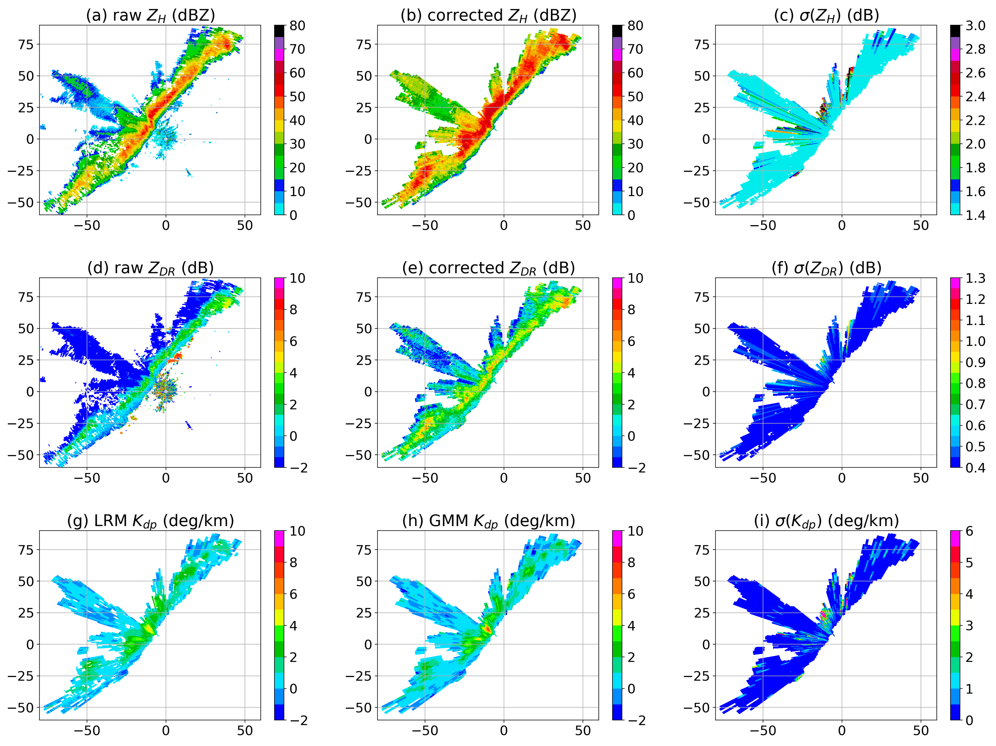
3.1. Clutter Removal

The noise and residual clutter in $Z_H$, $Z_{DR}$, and ${\mathrm{\Phi }}_{dp}$ need to be removed prior to the rain rate estimation. As this step is independent of the $K_{dp}$ estimation and attenuation correction, the existing techniques may be adopted with respect to the radar specifications and research purposes [44,45,46]. In this study, a simplified Gaussian mixture method is applied to the MZZU radar data [37]. The range profile of ${\mathrm{\Phi }}_{dp}$ is first separated into multiple clusters, each of which corresponds to a data segment. Secondly, a segment is classified into weather and clutter by comparing the weight of each data segment with the pre-set thresholds. Thirdly, the clusters are evaluated based on the types of the segments. Fourthly, azimuthally isolated data points are removed to yield the clean ${\mathrm{\Phi }}_{dp}$ data. Finally, the $Z_H$ and $Z_{DR}$ data are processed referring to the clean ${\mathrm{\Phi }}_{dp}$.

3.2. $K_{dp}$ Estimation

The prevalent method for $K_{dp}$ estimation is a linear regression model (LRM), which fits a first-order polynomial function to the range profile of ${\mathrm{\Phi }}_{dp}$ [12]. It is formulated as

$$y={\beta }_0+{\beta }_{1}x+ϵ,$$

(1)

where ${\mathrm{\Phi }}_{dp}$ is denoted as y, the radar range is denoted as x, ${\beta }_0$ is the intercept, ${\beta }_1$ is the slope, and $ϵ$ is the error. The error $ϵ$ is individually and independently distributed, and drawn from a zero-mean Gaussian distribution with variance ${\sigma }^2$. The specific differential phase $K_{dp}$ is then estimated by the slope ${\beta }_1$, yielding:

$$\mathrm{LRM}{K}_{dp}={\beta }_1=\frac{{\sum }_{i=1}^n(x_i-\overline{x})y_i}{{\sum }_{i=1}^n{(x_i-\overline{x})}^2},$$

(2)

where n is the number of gates and $\overline{x}$ is the mean value in the n gates. As $ϵ$ is the only stochastic variable, i.e., ${\sigma }^2(y)={\sigma }^2$, the variance of $K_{dp}$ is estimated as

$$\mathrm{LRM}\sigma (K_{dp})={\sigma }^2({\beta }_1)=\frac{{\sigma }^2}{{\sum }_{i=1}^n{(x_i-\overline{x})}^2}.$$

(3)

For linear polarization, ${\sigma }^2$ is related to the variance in phase for each of the two polarizations [47], leading to $\sigma ({\mathrm{\Phi }}_{dp})=2.61°$ using 32 pulses for the MZZU radar. By substituting to Equation (3), it yields $\sigma (K_{dp})=0.1$ deg km${}^{-1}$ if we apply 31 range gates with a gate spacing of 260 m. Moreover, as the variance of $K_{dp}$ is a constant inherited from ${\sigma }^2({\mathrm{\Phi }}_{dp})$, lower $K_{dp}$ has higher coefficient of variation $\left(\sigma (K_{dp})/K_{dp}\right)$ compared to higher $K_{dp}$. For example, if the radar collects a datum of $K_{dp}=0.1$ deg km${}^{-1}$, its coefficient of variation is about 100%, whereas the coefficient of variation is only 10% for $K_{dp}=1.0$ deg km${}^{-1}$.

Nevertheless, it is clear that the assumption of ${\sigma }^2(\widehat{y})={\sigma }^2$ may not always hold when the randomness of y is considered in the data generation model. If the variable y follows a probability distribution with mean $\overline{y}$ and variance ${\sigma }^2(y)$, the estimate $\widehat{y}$ is

$$\begin{array}{cc}\hfill \widehat{y}& =\overline{y},\hfill \end{array}$$

(4)

$$\begin{array}{cc}\hfill {\sigma }^2(\widehat{y})& ={\sigma }^2(y)+{\sigma }^2.\hfill \end{array}$$

(5)

From Equations (4) and (5), we can see that the data generation model leads to a better representation of the random error of ${\mathrm{\Phi }}_{dp}$. Therefore, [37] proposed a probabilistic method based on a Gaussian mixture model for $K_{dp}$ estimation using the MZZU radar data. The Gaussian mixture method (GMM) can not only estimate the expected values of $K_{dp}$ by differentiating the conditional expectation of ${\mathrm{\Phi }}_{dp}$, but also calculate the variance of $K_{dp}$ by regarding the errors in the calculation of the first derivative of ${\mathrm{\Phi }}_{dp}$.

In this method, the range gate and the ${\mathrm{\Phi }}_{dp}$ data are fitted into a Gaussian mixture, i.e.,

$$p(x,y)=\sum _{i=1}^m{w}_i\mathcal{N}(x,y;{\mathit{\mu }}_{\mathit{i}},{{\Sigma }}_{\mathit{i}}),$$

(6)

where x is the range gate, y is the ${\mathrm{\Phi }}_{dp}$, m is the number of components in the mixture, $w_i$ is a weight with ${\sum }_{i=1}^m{w}_i=1$, and $\mathcal{N}(x,y;{\mathit{\mu }}_{\mathbf{i}},{{\Sigma }}_{\mathbf{i}})$ represents a multi-variant Gaussian distribution with mean ${\mathit{\mu }}_{\mathbf{i}}=\left(\begin{array}{c}{\mu }_i^x\\ {\mu }_i^y\end{array}\right)$ and covariance ${{\Sigma }}_{\mathbf{i}}=\left(\begin{array}{cc}{{\Sigma }}_i^{xx}& {{\Sigma }}_i^{xy}\\ {{\Sigma }}_i^{yx}& {{\Sigma }}_i^{yy}\end{array}\right)$. The parameters are iteratively computed by an Expectation-Maximization algorithm. Subsequently, the probability of y conditioned on x is also a Gaussian mixture, yielding

$$\begin{array}{cc}\hfill p(y|x)& =\sum _{i=1}^m{w}_i^{y|x}\mathcal{N}(y;{\mu }_i^{y|x},{{\Sigma }}_i^{y|x}),\hfill \end{array}$$

(7)

$$\begin{array}{cc}\hfill w_i^{y|x}& =\frac{w_i\mathcal{N}(x;{\mu }_i^x,{{\Sigma }}_i^{xx})}{{\sum }_{j=1}^m{w}_j\mathcal{N}(x;{\mu }_j^x,{{\Sigma }}_j^{xx})},\hfill \end{array}$$

(8)

$$\begin{array}{cc}\hfill {\mu }_i^{y|x}& ={\mu }_i^y+{{\Sigma }}_i^{yx}{({{\Sigma }}_i^{xx})}^{-1}(x-{\mu }_i^x),\hfill \end{array}$$

(9)

$$\begin{array}{cc}\hfill {{\Sigma }}_i^{y|x}& ={{\Sigma }}_i^{yy}-{{\Sigma }}_i^{yx}{({{\Sigma }}_i^{xx})}^{-1}{{\Sigma }}_i^{xy},\hfill \end{array}$$

(10)

where $w_i^{y|x}$, ${\mu }_i^{y|x}$, and ${{\Sigma }}_i^{y|x}$ are the conditional weight, mean, and covariance, respectively.

The mean differential phase shift ${\mathrm{\Phi }}_{dp}$ is then retrieved by the mathematical expectation of Equation (7). Let $f_i(x)=w_i\mathcal{N}(x;{\mu }_i^x,{{\Sigma }}_i^{xx})$ and $f(x)={\sum }_{i=1}^m{f}_i(x)$, the expected value of y conditioned on x is expressed as

$$\begin{array}{cc}\hfill \mathrm{GMM}{\mathrm{\Phi }}_{dp}& =E(y|x)=\sum _{i=1}^m\frac{f_i(x)}{f(x)}(a_{i}x+b_i),\hfill \end{array}$$

(11)

$$\begin{array}{cc}\hfill a_i& ={{\Sigma }}_i^{yx}{({{\Sigma }}_i^{xx})}^{-1},\hfill \end{array}$$

(12)

$$\begin{array}{cc}\hfill b_i& ={\mu }_i^y-{{\Sigma }}_i^{yx}{({{\Sigma }}_i^{xx})}^{-1}{\mu }_i^x.\hfill \end{array}$$

(13)

Meanwhile, its variance is given as

$${\sigma }^2(y|x)=\sum _{i=1}^m{w}_i^{y|x}\left[{{\Sigma }}_i^{y|x}+{\left({\mu }_i^{y|x}\right)}^2\right]-{\left(\sum _{i=1}^m{w}_i^{y|x}{\mu }_i^{y|x}\right)}^2.$$

(14)

Substituting Equation (14) to Equation (5), the variance of ${\mathrm{\Phi }}_{dp}$ is finally obtained by

$$\mathrm{GMM}{\sigma }^2({\mathrm{\Phi }}_{dp})={\sigma }^2(\widehat{y}|x)={\sigma }^2+\sum _{i=1}^m{w}_i^{y|x}\left[{{\Sigma }}_i^{y|x}+{\left({\mu }_i^{y|x}\right)}^2\right]-{\left(\sum _{i=1}^m{w}_i^{y|x}{\mu }_i^{y|x}\right)}^2.$$

(15)

For simplicity, we assume that $\sigma$ is 2.61 deg km${}^{-1}$ for the MZZU radar.

By taking the derivative of Equation (11) with respect to the radar range x, $K_{dp}$ is retrieved by

$$\mathrm{GMM}{K}_{dp}=E^{\prime }(y|x)=\frac{1}{f^2(x)}\left\{\sum _{i=1}^m\sum _{j=1}^m{f}_i(x)f_j(x)\left[\left(\frac{x-{\mu }_j^x}{{{\Sigma }}_j^{xx}}-\frac{x-{\mu }_i^x}{{{\Sigma }}_i^{xx}}\right)(a_{i}x+b_i)+a_i\right]\right\},$$

(16)

Moreover, the variance of $K_{dp}$ is approximated by a Taylor series expansion, i.e.,

$$\mathrm{GMM}{\sigma }^2(K_{dp})={\sigma }^2({\widehat{y}}^{\prime }|x)\approx {\left[E^{″}(y|x)\right]}^2{\sigma }^2({\varphi }_{dp})={(K_{dp}^{\prime })}^2{\sigma }^2({\varphi }_{dp}),$$

(17)

where ${\sigma }^2({\mathrm{\Phi }}_{dp})$ is given in Equation (15). The derivative of $K_{dp}$ is expressed as

$$K_{dp}^{\prime }=2\sum _{i=1}^m{a}_i{(w_i^{y|x})}^{\prime }+\sum _{i=1}^m(a_{i}x+b_i){(w_i^{y|x})}^{\prime \prime },$$

(18)

where

$$\begin{array}{cc}\hfill {\left(w_i^{y|x}\right)}^{\prime }& =\frac{g_i(x)}{f^2(x)}=\frac{1}{f^2(x)}\sum _{j=1}^m{f}_j(x)f_i(x)\left(\frac{x-{\mu }_j^x}{{{\Sigma }}_j^{xx}}-\frac{x-{\mu }_i^x}{{{\Sigma }}_i^{xx}}\right),\hfill \end{array}$$

(19)

$$\begin{array}{cc}\hfill {\left(w_i^{y|x}\right)}^{″}& =\frac{g_i^{\prime }(x)f(x)-2f^{\prime }(x)g_i(x)}{f^3(x)},\hfill \end{array}$$

(20)

$$\begin{array}{cc}\hfill f^{\prime }(x)& =-\sum _{j=1}^m\frac{x-{\mu }_j^x}{{{\Sigma }}_j^{xx}}{f}_j(x),\hfill \end{array}$$

(21)

$$\begin{array}{cc}\hfill g_i^{\prime }(x)& =\sum _{j=1}^m{f}_j(x)f_i(x)\left(\frac{x-{\mu }_i^x}{{{\Sigma }}_i^{xx}}-\frac{x-{\mu }_j^x}{{{\Sigma }}_j^{xx}}+\frac{1}{{{\Sigma }}_j^{xx}}-\frac{1}{{{\Sigma }}_i^{xx}}\right).\hfill \end{array}$$

(22)

It can be found that $K_{dp}$ is estimated by the derivative of the mathematical expectation of ${\mathrm{\Phi }}_{dp}$ conditioned on the range x, while the variance of $K_{dp}$ is related to the range derivative of $K_{dp}$ and the variance of ${\mathrm{\Phi }}_{dp}$.

It is known that the X-band radar data are affected by ambiguous ${\mathrm{\Phi }}_{dp}$ and backscattering differential phase shift ${\delta }_{co}$ ([37], Figure 5). To correct these errors, we compare the means of two consecutive clusters along the range. If the latter cluster has a mean larger than the former one by 80${}^{°}$, the latter one is labeled as ambiguous ${\mathrm{\Phi }}_{dp}$ and unfolded by adding 180${}^{°}$. On the other hand, the latter cluster is removed due to ${\delta }_{co}$ if its mean is 85${}^{°}$ smaller than the former one or if its weight is less than 0.0501.

Moreover, a finite impulse response (FIR) filter is applied to reduce the $K_{dp}$ variances [48]. In [37], the filtering for each ray is optimized in terms of relative square error, leading to a window length between 29 and 33 gates for the MZZU radar. As discussed in [49], the spatial resolution gives a strong correlation with the temporal resolution, giving a relation of $r=5t^{0.3}$ where t in min and r in km. If the radar data are updated every 4.5 min, the spatial resolution requires a minimum of 7.85 km, equivalent to 31 range gates.

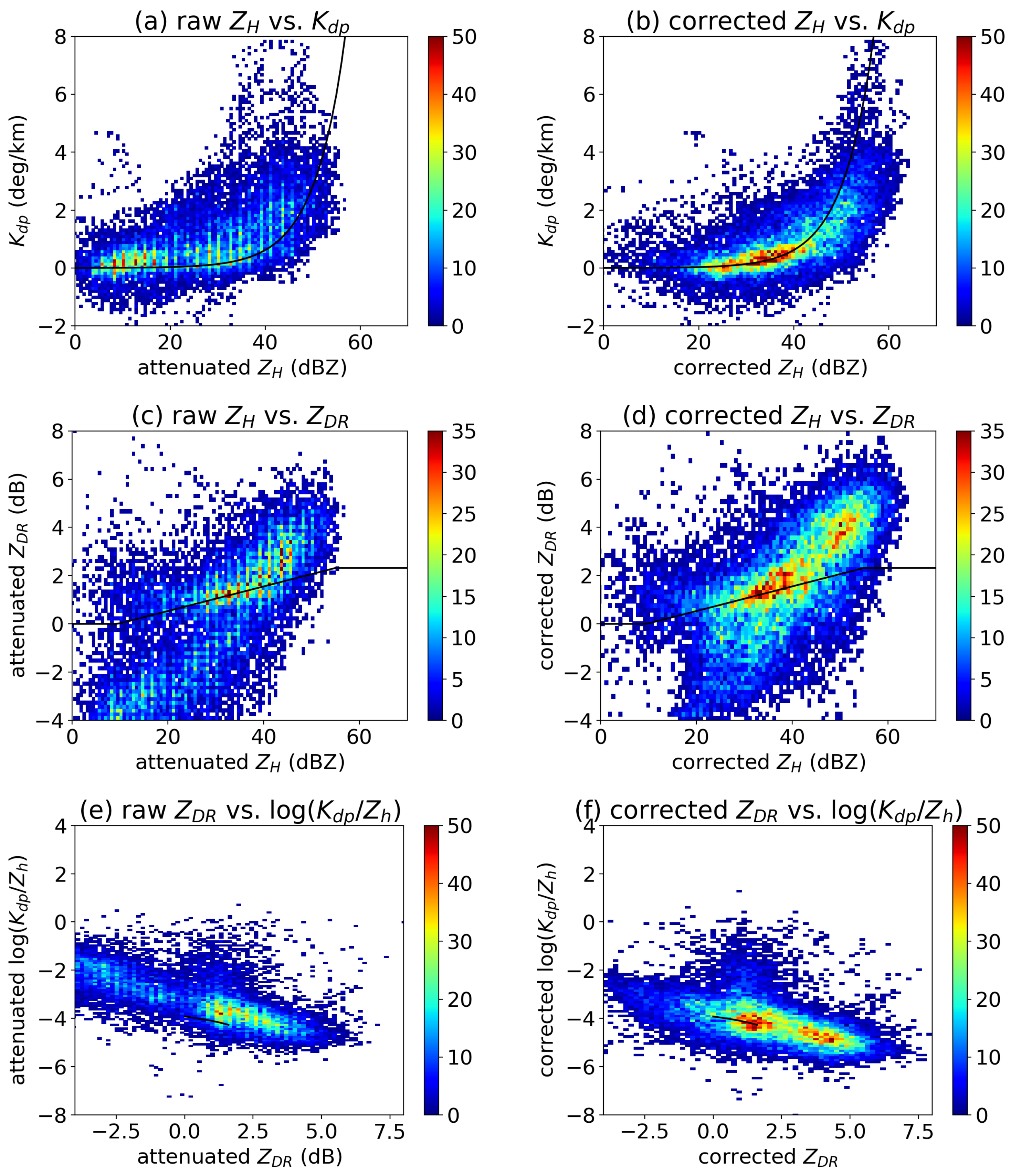
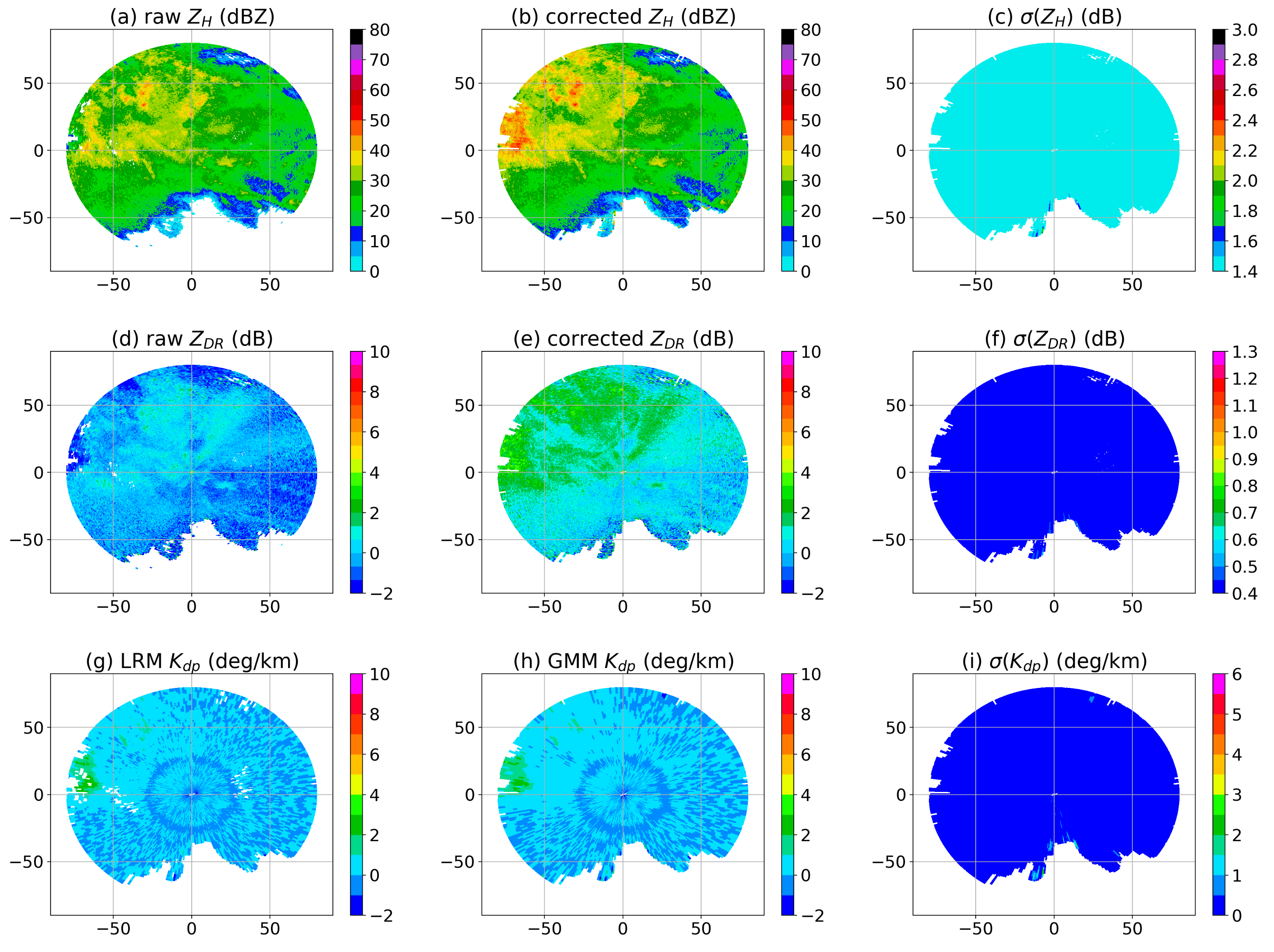
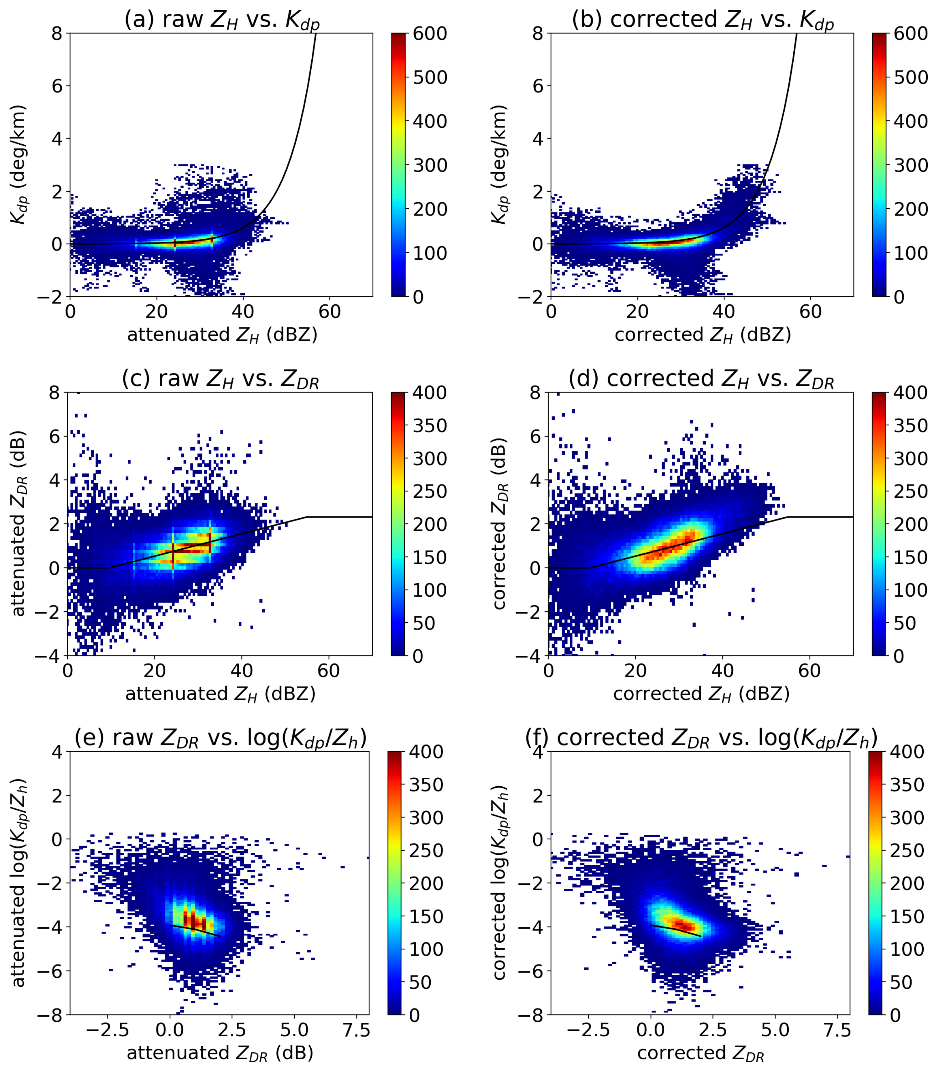
3.3. Attenuation Correction

It is important to do the attenuation correction before the rain rate estimation, as the Mie scattering significantly affects the power measurements at X-band frequency. The attenuation effects at X-band are significant due to the scattering and absorption of raindrops along the wave propagation path [12]. The T-matrix simulations show that $A_H$ and $A_{DP}$ at X-band are about 10 times and 5 times larger than those at S- and C-band, respectively [13,50]. Nevertheless, $K_{dp}$ is insensitive to the attenuation effects, and therefore useful for determining $A_H$ and $A_{DP}$ as a function of range. In this section, we apply GMM $K_{dp}$ to the attenuation correction for the MZZU radar.

The specific attenuation is related to the integral of the raindrop size distribution (DSD) and the imaginary part of forwarding scattering amplitude, which is defined as

$$A_{H,V}=4.343\times {10}^{-3}{\int }_0^{\infty }N(D)·\Im \left\{f_{hh,vv}(0,D)\right\}dD,(\mathrm{dB}{\mathrm{km}}^{-1})$$

(23)

where D is the raindrop size in millimeter, $N(D)$ is the drop spectrum in m${}^{-3}$mm${}^{-1}$, $\Im \{·\}$ is the imaginary part and $f_{hh,vv}(0,D)$ are the forward scattering amplitudes at the horizontal and vertical polarizations, respectively. The specific differential attenuation is then given as

$$A_{DP}=A_H-A_V.(\mathrm{dB}{\mathrm{km}}^{-1})$$

(24)

As $K_{dp}$ is also related to the forward scattering amplitude, $A_H$ and $A_{DP}$ may be calculated by an exponential function of $K_{dp}$, respectively, i.e.,

$$\begin{array}{cc}\hfill A_H& =\alpha K_{dp}^{{\gamma }_1},\hfill \end{array}$$

(25)

$$\begin{array}{cc}\hfill A_{DP}& =\beta K_{dp}^{{\gamma }_2}.\hfill \end{array}$$

(26)

where $\alpha$, $\beta$, ${\gamma }_1$, and ${\gamma }_2$ are constant coefficients. The variables $Z_H$ and $Z_{DR}$ are then corrected by

$$\begin{array}{cc}\hfill Z_H^{att}& =Z_H^{raw}+2{\int }_0^r{A}_H(s)ds,\hfill \end{array}$$

(27)

$$\begin{array}{cc}\hfill Z_{DR}^{att}& =Z_{DR}^{raw}+2{\int }_0^r{A}_{DP}(s)ds.\hfill \end{array}$$

(28)

where $Z_H^{att}$ and $Z_{DR}^{att}$ are corrected $Z_H$ and $Z_{DR}$, respectively, and $Z_H^{raw}$ and $Z_{DR}^{raw}$ are raw $Z_H$ and $Z_{DR}$, respectively. For simplicity, we assume the coefficients ${\gamma }_1$ and ${\gamma }_2$ are unity, leading to a ${\varphi }_{dp}$-based attenuation correction method [13],

$$\begin{array}{cc}\hfill Z_H^{att}& =Z_H^{raw}+\alpha [{\varphi }_{dp}(r)-{\varphi }_{dp}(0)],\hfill \end{array}$$

(29)

$$\begin{array}{cc}\hfill Z_{DR}^{att}& =Z_{DR}^{raw}+\beta [{\varphi }_{dp}(r)-{\varphi }_{dp}(0)],\hfill \end{array}$$

(30)

where ${\varphi }_{dp}(0)$ is the initial ${\varphi }_{dp}$, and ${\varphi }_{dp}(r)$ is the re-constructed ${\varphi }_{dp}$ at the rth gate. The coefficients $\alpha$ and $\beta$ depend on the radar frequency, DSD and drop shape [23,51]. With the assumption of the drop shape of [13,52] calculate $\alpha$ and $\beta$ using the T-matrix simulation based on observed DSDs. Following this work, we derive $\alpha$ and $\beta$ as 0.25 and 0.05, respectively, using the MZZU-RG comparison dataset. The coefficients are similar to the ones presented in the previous studies [14,53].

From Equations (29) and (30), the variance of corrected $Z_H$ and $Z_{DR}$ are related to the variance of ${\varphi }_{dp}$ and the variance of raw $Z_H$ and $Z_{DR}$, respectively. By assuming that $Z_H$, $Z_{DR}$, and ${\varphi }_{dp}$ are independent, we have

$$\begin{array}{c}\hfill {\sigma }^2\left(Z_H^{att}\right)={\sigma }^2\left(Z_H^{raw}\right)+{\alpha }^2{\sigma }^2\left[{\varphi }_{dp}(r)\right],\end{array}$$

(31)

$$\begin{array}{c}\hfill {\sigma }^2\left(Z_{DR}^{att}\right)={\sigma }^2\left(Z_{DR}^{raw}\right)+{\beta }^2{\sigma }^2\left[{\varphi }_{dp}(r)\right],\end{array}$$

(32)

where $\sigma \left(Z_H^{raw}\right)$ and $\sigma \left(Z_{DR}^{raw}\right)$ are 1.36 dB and 0.436 dB for the MZZU radar, respectively. Equations (31) and (32) indicate that the attenuation correction may increase the uncertainties for $Z_H$ and $Z_{DR}$, and consequently produce higher errors in the $Z_H$ and/or $Z_{DR}$-based rain rates. Finally, we use the $Z_H$ and $Z_{DR}$ after the attenuation correction in the rain rate estimation, while the variables in linear units are calculated by

$$\begin{array}{cc}\hfill Z_H& =10\times {log}_{10}(Z_h),\hfill \end{array}$$

(33)

$$\begin{array}{cc}\hfill Z_{DR}& =10\times {log}_{10}(Z_{dr}),\hfill \end{array}$$

(34)

where $Z_h$ is in mm${}^6$m${}^{-3}$ and $Z_{dr}$ is unitless.

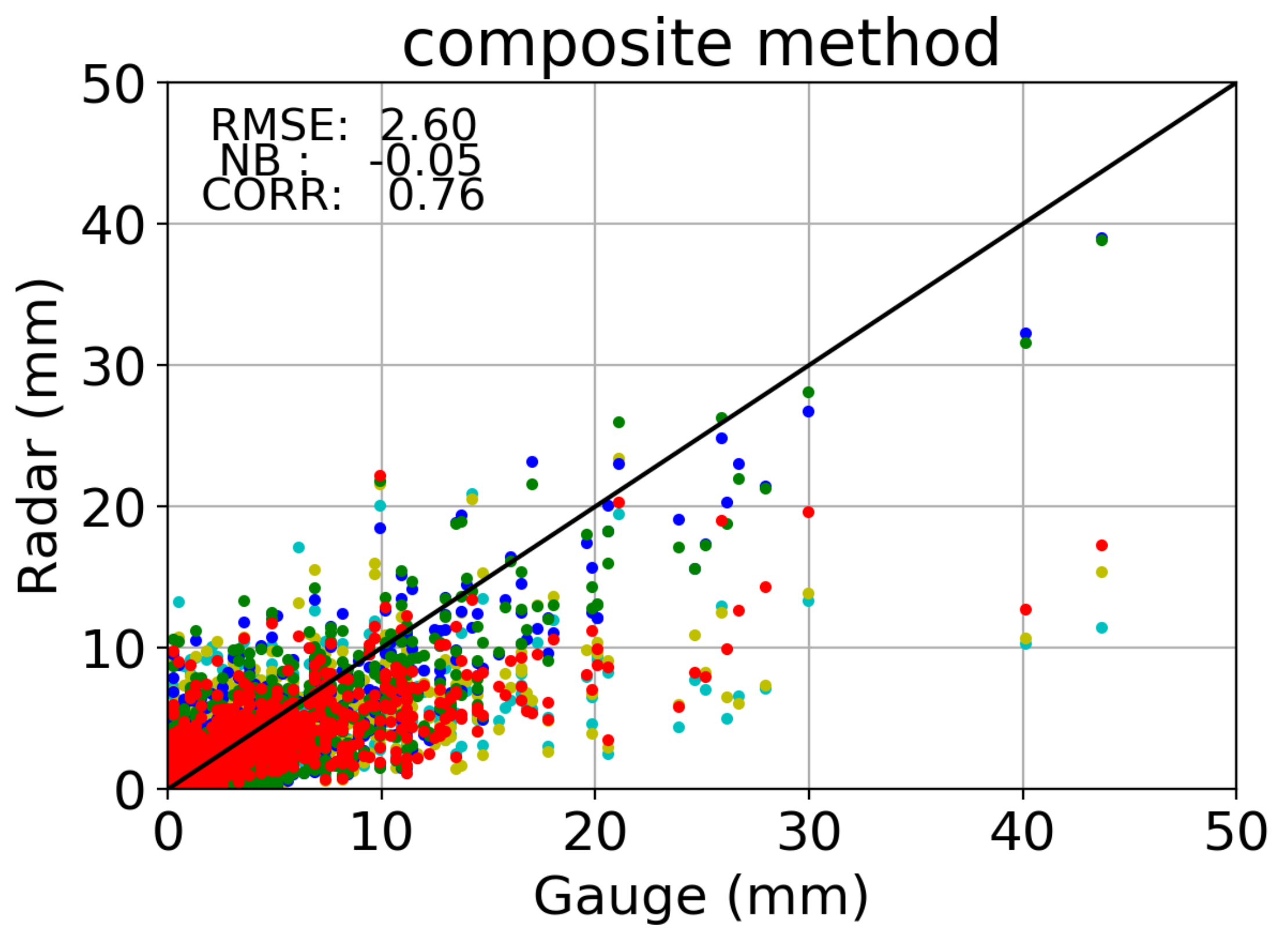
4. Rain Rate Estimation

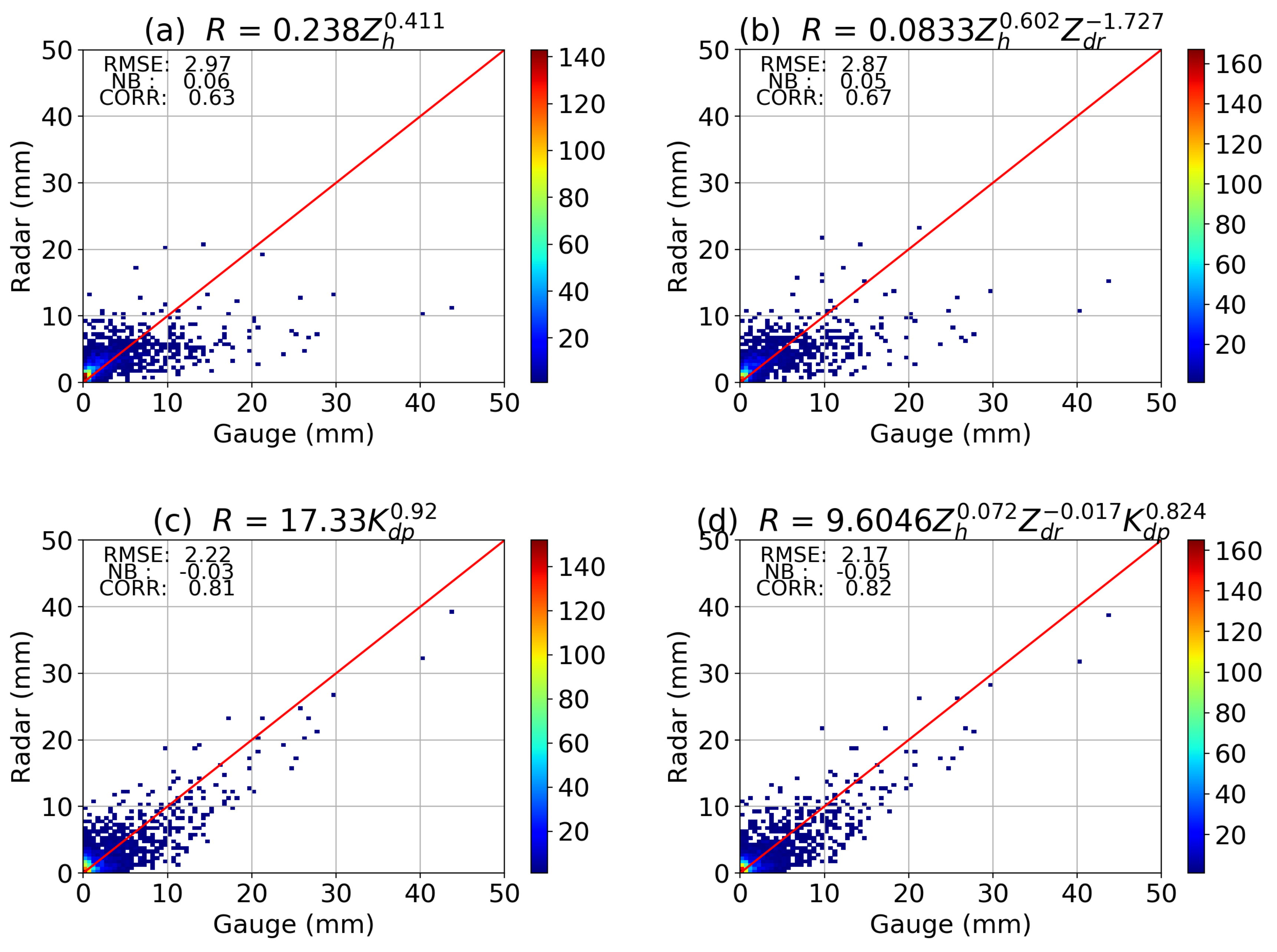
In this section, the rain rate estimation algorithms are first derived from the MZZU-RG comparison data, and the statistical uncertainties $\sigma (R)$ are then calculated by considering the propagation of the uncertainties of $Z_h$, $Z_{dr}$, and $K_{dp}$ in the power-law relations. The algorithms of $R(Z_h)$, $R(Z_h,Z_{dr})$, $R(K_{dp})$, and $R(Z_h,Z_{dr},K_{dp})$ are optimized in terms of the root mean square error (RMSE). It is defined as

$$\mathrm{RMSE}=\sqrt{\frac{{\sum }_{i=1}^N{\left(R_i-G_i\right)}^2}{N}},$$

(35)

where N is the sample size, $R_i$ is the radar hourly rain amount, and $G_i$ is the hourly gauge data. In addition to RMSE, the normalized bias (NB) and Pearson correlation coefficient (CORR) are also calculated to analyze the accuracy of the algorithms. They are given as

$$\begin{array}{cc}\hfill \mathrm{NB}& =\frac{{\sum }_{i=1}^N(R_i-G_i)}{{\sum }_{i=1}^N{G}_i},\hfill \end{array}$$

(36)

$$\begin{array}{cc}\hfill \mathrm{CORR}& =\frac{{\sum }_{i=1}^N(R_i-\overline{R})(G_i-\overline{G})}{\sqrt{{\sum }_{i=1}^N{(R_i-\overline{R})}^2}\sqrt{{\sum }_{i=1}^N{(G_i-\overline{G})}^2}},\hfill \end{array}$$

(37)

where $\overline{R}$ and $\overline{G}$ are the sample means for radar and gauge, respectively.

4.1. Retrieval of R

The linear radar reflectivity $Z_h$ is the sixth order moments of DSD [12,54], while the rain rate R is about 3.67th order moment. Consequently, the rain rate may be retrieved via a power-law relation of $Z_h$ and R [55],

$$R(Z_h)=0.238Z_h^{0.411},$$

(38)

where $Z_h$ is in units of mm${}^6$m${}^{-3}$, and the coefficients of 0.238 and 0.411 are optimized for the MZZU-RG data. To reduce the sensitivity to the variability of DSD, $Z_{dr}$ is incorporated into $R(Z_h)$, leading to the $R(Z_h,Z_{dr})$ algorithm, i.e.,

$$R(Z_h,Z_{dr})=0.0833Z_h^{0.602}{Z}_{dr}^{-1.727}.$$

(39)

Nevertheless, the $R(Z_h)$ and $R(Z_h,Z_{dr})$ algorithms suffer from the absolute radar calibration errors and the Mie effects at X-band [56]. As $K_{dp}$ is a phase measurement, the $R(K_{dp})$ algorithm is often used to improve the accuracy of the rain rate estimation at X-band, yielding

$$R(K_{dp})=17.33K_{dp}^{0.92}.$$

(40)

It is noted that the $R(K_{dp})$ algorithm may have a lower range resolution than $R(Z_h)$ and $R(Z_h,Z_{dr})$ due to the window smoothing. Therefore, $Z_h$, $Z_{dr}$, and $K_{dp}$ are combined to obtain a tradeoff between the accuracy and the resolution. The $R(Z_h,Z_{dr},K_{dp})$ algorithm is given as

$$R(Z_h,Z_{dr},K_{dp})=9.6046Z_h^{0.072}{Z}_{dr}^{-0.017}{K}_{dp}^{0.824}.$$

(41)

Figure 1 gives a comparison between the radar rain rates and the RG data obtained by Equations (38)–(41). The scatterplots allow an easy examination of the algorithms, especially when the one-to-one line (red line) is included. The rain rates that perfectly match the RG data would fall on this line.

In Figure 1, the radar data of 1151 h contain 1940 points available for the four RGs. The majority of the points are associated with small R (light rain), followed by a sizeable number of points with medium R (moderate rain). The points with high R (heavy rain) only take a small portion but make a significant contribution to the total rain amounts. Looking at the scatterplots in more detail, we can see that $R(Z_h)$ (Figure 1a) gives a clear underestimation with a considerable amount of the points below the red line. As a result of the effects of the Mie scattering, negative outliers are clearly identified in the region of RG larger than 20 mm and radar R less than 10 mm. In addition, there are a small number of points above the red curve, leading to large RMSE of 2.97 and small CORR of 0.63. Moreover, the $R(Z_h,Z_{dr})$ algorithm (Figure 1b) has a similar trend to $R(Z_h)$ due to the Mie effect, giving RMSE of 2.87, NB of 0.05 and CORR of 0.67.

The $R(K_{dp})$ and $R(Z_h,Z_{dr},K_{dp})$ algorithms improve the estimation of R when compared to $R(Z_h)$ and $R(Z_h,Z_{dr})$. The scatterplots in Figure 1c,d show a better concentration on the red line with noticeable changes for higher R. According to Figure 1c, $R(K_{dp})$ has improved the R in the bottom-right region, yielding remarkable RMSE and ${\rho }_{RG}$ at 2.22 and 0.81, respectively. The discrepancy still exist in the region of heavy rain, particularly for R larger than 20 mm. Furthermore, $R(Z_h,Z_{dr},K_{dp})$ in Figure 1d are similar to $R(K_{dp})$ in Figure 1c, while the points with higher R concentrate on the red line. Consequently, the RMSE and CORR of $R(Z_h,Z_{dr},K_{dp})$ are better than those of $R(K_{dp})$. In contrast, the NB of $R(Z_h,Z_{dr},K_{dp})$ is a little worse, leading to a value of −0.05.

4.2. Retrieval of $\sigma (R)$

By using the perturbation analysis [12], the statistical uncertainty $\sigma (R)$ in Equation (38) is given as

$$\begin{array}{cc}\hfill \frac{\sigma (R)}{R}& =0.411\frac{\sigma (Z_h)}{Z_h},\hfill \end{array}$$

(42)

$$\begin{array}{cc}\hfill \sigma (Z_H)& =10{log}_{10}\left[1+\frac{\sigma (Z_h)}{Z_h}\right],\hfill \end{array}$$

(43)

where $Z_H=10{log}_{10}(Z_h)$. Similarly, the variance of $R(Z_h,Z_{dr})$ is expressed as

$$\begin{array}{cc}\hfill \frac{{\sigma }^2(R)}{R^2}& ={\left[0.602\frac{\sigma (Z_h)}{Z_h}\right]}^2+{\left[1.727\frac{\sigma (Z_{dr})}{Z_{dr}}\right]}^2,\hfill \end{array}$$

(44)

$$\begin{array}{cc}\hfill \sigma (Z_{DR})& =10{log}_{10}\left[1+\frac{\sigma (Z_{dr})}{Z_{dr}}\right],\hfill \end{array}$$

(45)

where $Z_{DR}=10{log}_{10}(Z_{dr})$. It is noticeable that $\sigma (R)$ in Equations (42) and (44) are independent of the absolute values of $Z_h$ and $Z_{dr}$. In contrast, $K_{dp}$ is in a linear scale, and thus the statistical uncertainty $\sigma (R)$ is related to $K_{dp}$ and $\sigma (K_{dp})$, leading to the expression of

$$\frac{\sigma (R)}{R}=0.92\frac{\sigma (K_{dp})}{K_{dp}}.$$

(46)

Finally, the variance of R in Equation (41) is derived as

$$\frac{{\sigma }^2(R)}{R^2}={\left[0.072\frac{\sigma (Z_h)}{Z_h}\right]}^2+{\left[0.017\frac{\sigma (Z_{dr})}{Z_{dr}}\right]}^2+{\left[0.824\frac{\sigma (K_{dp})}{K_{dp}}\right]}^2.$$

(47)

It is known that $R(K_{dp})$, $R(Z_h,Z_{dr})$, and $R(Z_h,Z_{dr},K_{dp})$ are less sensitive to the DSD variability than the conventional $R(Z_h)$. However, the polarimetric algorithms yield higher statistical uncertainty of R due to the uncertainties of $Z_{dr}$ and $K_{dp}$ [31]. This problem is obvious when R is small. As shown in Figure 1, $R(K_{dp})$ and $R(Z_h,Z_{dr},K_{dp})$ give a significant improvement over $R(Z_h)$ and $R(Z_h,Z_{dr})$ for R exceeding 10 mm h${}^{-1}$, whereas $R(Z_h)$ and $R(Z_h,Z_{dr})$ have a better estimation for R less than 5 mm h${}^{-1}$. The explicit solution is to combine all the available algorithms by considering their statistical errors at a particular location in a certain period of time. For example, the rain rate estimation algorithms can be selected based on the reflectivity thresholds to reduce the effects of the statistical uncertainty for lower rain rates [57].

Nevertheless, it is difficult to determine the hard thresholds for various rain rate estimation algorithms, and the thresholds may be biased due to the statistical uncertainties of $Z_h$, $Z_{dr}$, and $K_{dp}$, particularly for X-band radars. The rain rate algorithms can then be combined softly by adding a weight for each rain rate algorithm, leading to a composite method [58,59]. In this method, the weight is calculated by multiplying the inverse of the statistical uncertainty $\sigma (R)$ by a normalized constant $a_i$, i.e.,

$$R=\sum _{i=1}^n\frac{a_i}{\sigma (R_i)}{R}_i,$$

(48)

where ${\sum }_{i=1}^n\frac{a_i}{\sigma (R_i)}=1$ and $R_i$ includes $R(Z_h)$, $R(Z_h,Z_{dr})$, $R(K_{dp})$, and $R(Z_h,Z_{dr},K_{dp})$.

It can be seen that this method uses the statistical errors as a function of range gates to yield the variability of R. The previous research often analyzes the errors of $Z_h$, $Z_{dr}$, and $K_{dp}$ from a view of signal processing [47], leading to a constant $\sigma (R)/R$ except for $R(K_{dp})$. In this study, we also consider the propagation of the statistical uncertainties of $Z_h$, $Z_{dr}$, and $K_{dp}$ in the rain rate estimation. To determine the coefficient $a_i$ in Equation (48), it is straightforward to set $a_i$ as the value of $\sigma (R_i)$ if the corresponding algorithm has the smallest $\sigma (R_i)$ weighted by the absolute values $A_i$ of the polarimetric values. Therefore, the composite method selects the rain rate with the smallest $\sigma (R)$ as derived from the four algorithms:

$$R=arg\underset{R_i}{min}{A}_i\sigma (R_i),$$

(49)

where $A_i$ is equal to $Z_h$, $Z_{dr}$, and $K_{dp}$, respectively.

Figure 2 compares the rain rates estimated by radar algorithms in Equations (38)–(41) and Equation (49) to the RG data. The accompanying colors show the radar algorithms of $R(K_{dp})$ (blue), $R(Z_h)$ (cyan), $R(Z_h,Z_{dr})$ (yellow), $R(Z_h,Z_{dr},K_{dp})$ (green), and the composite method (red). Consistent with the RG data, the entire body of rain rates by the composite method is predominantly made up of light rain with only a small quantity of moderate rain and heavy rain making up the remainder. Among the five radar algorithms, the composite method yields the best performance for light rain, showing a narrow spread around the reference line. Furthermore, the composite method has a slightly higher variation for moderate rain when compared to $R(K_{dp})$, as the red dots tend to less close to the reference line than the blue dots. Nevertheless, the rain rates by the composite method well concentrate on the reference line for heavy rain.

When we study the associated RMSE, NB, and CORR, it is apparent that $R(K_{dp})$, $R(Z_h,Z_{dr},K_{dp})$, and the composite method all have their advantages. The RMSE and CORR for the composite method are the best among the five algorithms, yielding improved results of 2.08 and 0.84, respectively. In particular, the RMSE for the composite has a significant improvement over $R(K_{dp})$ and $R(Z_h,Z_{dr},K_{dp})$. However, $R(K_{dp})$ and $R(Z_h,Z_{dr},K_{dp})$ still outperform the composite method in terms of NB.

5. Case Studies

The detailed analyses of individual cases are important for the accuracy assessment for the quality control and rain rate estimation for the MZZU radar. We have selected two rainfall events, including a squall line event on 7 March 2017 and a prolonged rain event on 2–4 July 2016.

5.1. Squall Line Event: 7 March 2017

On 7 March 2017, a squall line developed along a southeastward advancing cold front, and eventually entered central Missouri in the evening. Meanwhile, the rotation of the base of a northeastward-ejecting upper trough led to a strong mid-level jet, which contributed to vertical shear profiles and large 0–1 km shear for the organized storms by coupling with an intensifying southwesterly low-level jet. The supercells and bowing structures embedded in the squall line produced mainly damaging wind and large hail, with a few tornadoes along the path.

Figure 3 illustrates the MZZU radar observations of the squall line event at 0411 UTC. It is clear that the plan position indicators (PPIs) of $Z_H$, $Z_{DR}$, and $K_{dp}$ depict a straight-line structure with a length of about 180 km and a width of 15–30 km. The squall line moved at a speed of 60–70 km h${}^{-1}$ in a direction normal to the northeast-southwest orientation of the line.

Figure 3g and h both show strong convective cells ($K_{dp}>3$ deg km${}^{-1}$) with horizontal widths of a few kilometers surrounded by moderate echoes ($1<K_{dp}<3$ deg km${}^{-1}$). Notably, GMM $K_{dp}$ (Figure 3h) presents a series of intense cells in the center of the line, with a maximum of greater than 8 deg km${}^{-1}$. The edge of the line center appears to be jagged with forward extending protrusions. By taking a closer look at the leading edge, we can see a bow echo with a horizontal scale of 10 km, where corrected $Z_H$ is more than 60 dBZ (Figure 3b), corrected $Z_{DR}$ is 4–6 dB (Figure 3e) and GMM $K_{dp}$ is about 2 deg km${}^{-1}$. These radar signatures signify the occurrence of hail, which is consistent with the surface hail report at Columbia, Boone County (38.95${}^{°}$ N, 92.33${}^{°}$ W) at the time of 9 min later than the radar PPIs. At either side of the center, a number of weaker convective cells are aligned along the line, showing a symmetric shape of the storm. In contrast, LRM $K_{dp}$ (Figure 3g) tends to yield an extended region of the convective cores, but the maximum $K_{dp}$ values are considerably lower. When compared to GMM $K_{dp}$, LRM $K_{dp}$ obscures the manifestations of the serrated leading edge and elongated rain cells, increasing difficulties for the analysis of the storm structure.

Moreover, the radar echoes for the trailing stratiform cannot be observed due to strong attenuation at X-band caused by the leading edge. Nevertheless, GMM $K_{dp}$ shows a narrow sector of the stratiform rain behind a notch-like concavity at the leading edge. The concave structure is also associated with the bow echo, which may be linked to the mid-level inflow that inserts into the back of the convective line. The trailing stratiform rain is characterized by low $K_{dp}$ and relatively small $K_{dp}$ gradients. Likewise, LRM $K_{dp}$ depicts a uniformly distributed signature for the stratiform rain. The blank regions within LRM $K_{dp}$ are produced by missing ${\mathrm{\Phi }}_{dp}$ data, since the signal-to-noise ratio is below the noise threshold. In contrast, the Gaussian mixture method can provide meaningful $K_{dp}$ via the joint probability density function of ${\mathrm{\Phi }}_{dp}$ at these regions, though the statistical uncertainty $\sigma (K_{dp})$ tends to be increased (Figure 3i).

The statistical uncertainty $\sigma (K_{dp})$ gives a further insight into the radar signatures of GMM $K_{dp}$. Figure 3i shows that $\sigma (K_{dp})$ is increased in the convective regimes due to significant $K_{dp}$ gradients. However, the largest $\sigma (K_{dp})$ is not well associated with the highest $K_{dp}$ value, but it occurs at a location between the leading edge and the trailing stratiform, with a large $K_{dp}$ gradient. It may imply that the significant $\sigma (K_{dp})$ is an indicator of the transition regimes [60], where the DSDs are unique. In addition, the trailing stratiform regimes have smaller $\sigma (K_{dp})$ compared to the leading convection due to relatively stable $K_{dp}$ values.

As illustrated in Figure 3a,d, raw $Z_H$ and $Z_{DR}$ are affected by the rain attenuation. In Figure 3a, the rear part of the leading edge shows raw $Z_H$ of 20–30 dBZ, weaker than the typical signatures of convective rain. Moreover, the attenuation effects lead to a $Z_H$ gap between the leading edge and the rain cell at the far range. On the other hand, raw $Z_{DR}$ (Figure 3d) is unrealistically lower than −1 dB after passing the front part of the leading edge. As $K_{dp}$ is immune to the attenuation, it is applicable for the attenuation correction via Equations (29) and (30). Figure 3b,e depict that corrected $Z_H$ and $Z_{DR}$ in the leading edge have been intensified by about 10–20 dBZ and 1–3 dB, respectively, while the gap in the trailing part is transformed to a region of stratiform rain. Moreover, it is notable that the strong attenuation produces a “V”-shape echo in the hail region at X: −20~−15 km and Y: 15~20 km. The high $K_{dp}$ values have given significant compensation to corrected $Z_H$ and $Z_{DR}$, leading to intense echoes in this region. However, the correction using GMM $K_{dp}$ has the radial effects, particularly for the regions with missing values in raw $Z_H$ and $Z_{DR}$. It may be due to the $K_{dp}$ smoothing and the constant $\alpha$ and $\beta$ in Equations (29) and (30), respectively.

The statistical uncertainties $\sigma (Z_H)$ and $\sigma (Z_{DR})$ inherit $\sigma (K_{dp})$ via Equations (31) and (32), and therefore $\sigma (Z_H)$ and $\sigma (Z_{DR})$ for corrected $Z_H$ and $Z_{DR}$ are larger than those for raw data. According to Figure 3c,f, $\sigma (Z_H)$ and $\sigma (Z_{DR})$ are significant at the regions of high $K_{dp}$ gradients, as $\sigma (Z_H)$ and $\sigma (Z_{DR})$ are positively related to $\sigma (K_{dp})$. In Figure 3c, it can be seen that $\sigma (Z_H)$ is negligible relative to the magnitude of corrected $Z_H$. When $\sigma (Z_H)$ reaches the maximum, it is less than 1% of the corresponding $Z_H$ magnitude. In contrast, $\sigma (Z_{DR})$ is on the same order as the magnitude of corrected $Z_{DR}$. At the point with the largest $\sigma (Z_{DR})$, the ratio of $\sigma (Z_{DR})$ and $Z_{DR}$ can reach more than 20%, which is much higher than the upper limit for $Z_{DR}$ error. Overall, the attenuation correction using GMM $K_{dp}$ introduces relatively large errors for $Z_{DR}$, leading to higher uncertainty when corrected $Z_{DR}$ is used to retrieve the rain rate.

To give a further evaluation of the attenuation correction, the corrected $Z_H$ and $Z_{DR}$ are compared to the self-consistency relations of $Z_H$, $Z_{DR}$, and $K_{dp}$ [12,21,23,53,61]. Self-consistency relations are related to the drop size distribution [62]. In this study, we adopt the Pruppacher–Beard linear fit [63], yielding the following relations for the X-band radar:

$$\begin{array}{c}\hfill Z_{DR}=\left\{\begin{array}{ccc}\hfill 0& & Z_H\le 9.5\hfill \\ \hfill 0.051Z_H-0.486& & 9.5<Z_H\le 55\hfill \\ \hfill 2.319& & Z_H\ge 55\hfill \end{array}\right.,\end{array}$$

(50)

$$\begin{array}{cc}\hfill K_{dp}& =1.37\times {10}^{-3}\times {10}^{0.068Z_H}\times {10}^{-0.042Z_{DR}},\hfill \end{array}$$

(51)

$$\begin{array}{cc}\hfill K_{dp}/Z_h& =1.2\times {10}^{-4}-4.1\times {10}^{-5}{Z}_{DR}(Z_{DR}<1.6),\hfill \end{array}$$

(52)

where $Z_H=10log{Z}_h$ and $Z_h$ is in mm${}^6$m${}^{-3}$.

Figure 4 compares the scatterplots of corrected $Z_H$, corrected $Z_{DR}$ and GMM $K_{dp}$ to the self-consistency relations in Equations (50)–(52). As depicted in Figure 4a, $K_{dp}$ increases greatly when raw $Z_H$ is above 30 dBZ, showing a large difference from the self-consistency relations. In contrast, in Figure 4b, there is a low and steady increase in $K_{dp}$ when $Z_H$ is between 10 and 40 dBZ, following a significant $K_{dp}$ jump when $Z_H$ is larger than 40 dBZ. The most noteworthy increase is recorded for $Z_H$ greater than 50 dBZ, where $K_{dp}$ rises dramatically from 4 to 8 deg km${}^{-1}$. Overall, the $Z_H$-$K_{dp}$ points after the correction have good agreement with the self-consistency relations.

In Figure 4c,e, the points of $Z_H$-$Z_{DR}$ and $Z_{DR}$-$K_{dp}$/$Z_h$ can be separated into two data clusters with high populations, which remain after the attenuation correction in Figure 4d,f. As shown in Figure 4d, the cluster concentrated on 2 dB has a steady increasing trend, which agrees with the self-consistency relations. However, the higher slope of the cluster indicates that the coefficient $\beta$ in Equation (30) is not optimal for the MZZU radar. On the other hand, the cluster centered at $Z_H$ of 50 dBZ and $Z_{DR}$ of 4 dBZ are likely produced by a mixture of rain and hail, as melting hail or raindrops with ice cores make a significant contribution to $Z_{DR}$. In addition to the $Z_H$-$K_{dp}$ and $Z_H$-$Z_{DR}$ relations, it is evident that the ratio of $K_{dp}$ and $Z_h$ also shows a dependency on $Z_{DR}$. As $Z_{DR}$ rises, $K_{dp}$/$Z_h$ tends to drop steadily, following a similar trend with the scattering simulation [54].

Through Equations (38)–(49), we can retrieve the rain rates and their uncertainties. As might be expected, $R(Z_h)$ (Figure 5a) and $R(Z_h,Z_{dr})$ (Figure 5b) give an underestimation at the center of the leading edge, with the maximum rain rates of no more than 40 mm h${}^{-1}$. In contrast, $R(K_{dp})$ (Figure 5c) and $R(Z_h,Z_{dr},K_{dp})$ (Figure 5d) produce the values as high as 100 mm h${}^{-1}$, indicating intensive rain cells. What remains truly remarkable is that $K_{dp}$-based algorithms yield the meaningful rain rate estimation in the hail-contaminated regions at X-band. Somewhat surprisingly however, according to Figure 5b–d, $R(Z_h,Z_{dr})$, $R(K_{dp})$, and $R(Z_h,Z_{dr},K_{dp})$ present some missing data in the trailing stratiform due to negative values in $Z_{DR}$ and $K_{dp}$.

According to Figure 5e, the composite method shows the rain rate results similar to $R(K_{dp})$ in the leading edge. Likewise, the statistical uncertainty (Figure 5f) for the composite method has given higher values in the transition regime, which is consistent with the uncertainty of $Z_H$, $Z_{DR}$, and $K_{dp}$. However, it is clear the trailing stratiform in the composite method is characterized by lower R, giving the improvement of rain rate estimation in this region.

It is found that the elongated shapes in the convective cores may be resulted from the radial effect of $R(K_{dp})$ as the $K_{dp}$ is estimated independently for each ray. Furthermore, the $K_{dp}$ is applied to the attenuation correction along the radial, and thus $R(Z_h,Z_{dr},K_{dp})$ gives the discontinuity in the azimuthal direction. However, the strong vertical winds have a large contribution to the raindrop size distribution as well as fall speed, leading to uneven rain in space. The updrafts may lift the smaller raindrops and enhance the coalescence process during the falling. Therefore, the rain rates increase when the updrafts exist in the area. On the other hand, the radar ray may spread after a number of range gates, while the radar variables and the resulting rain rates are averaged over the volume. If the small convective cells present in a few adjacent radar gates, the rain rates within these gates may be higher than the surrounding gates, giving the discontinuity in space.

In conclusion, the quality control is effective for $Z_H$, $Z_{DR}$, and $K_{dp}$ in the rain regions of the squall line event. The data of GMM $K_{dp}$, corrected $Z_H$ and $Z_{DR}$ can provide an insight into the storm structure, and the scatterplots are consistent with the self-consistency relations at X-band. Furthermore, it is evident that $R(K_{dp})$ and $R(Z_h,Z_{dr},K_{dp})$ have better results than $R(Z_h)$ and $R(Z_h,Z_{dr})$ at X-band, and the composite method gives some improvements in the trailing stratiform regime.

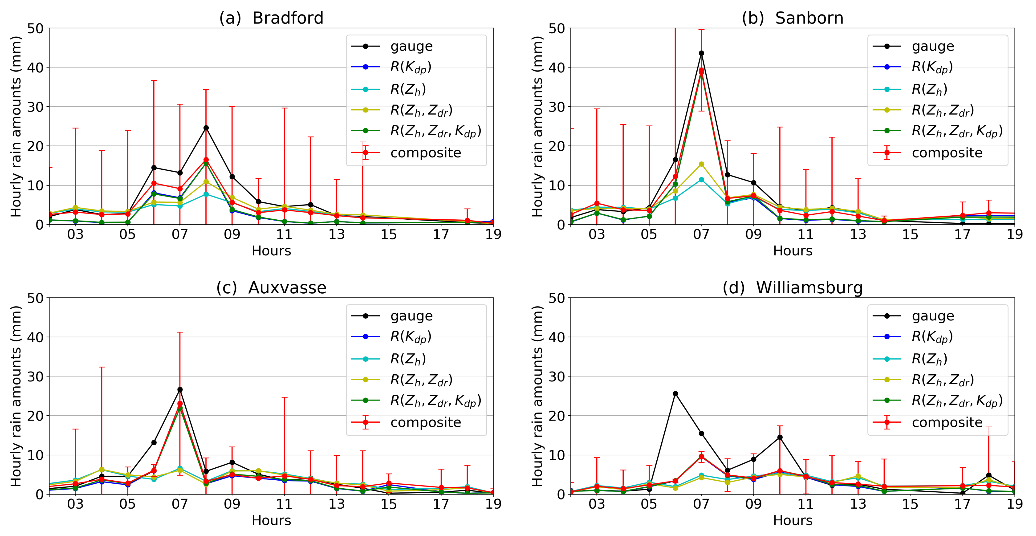
5.2. Prolonged Rain Event: 2–4 July 2016

From 2 July 2016, a weak lee-side trough formed at the southern Rocky Mountains and moved toward Missouri. It persisted over central Missouri and produced large areas of precipitation. Meanwhile, a cold front trailing from the low advanced southeastward across the radar surveillance area, causing convective rain and strong winds.

Figure 6 illustrates the radar PPIs at 0339 UTC on 3 July 2016, when the convection embedded in the stratiform is approaching. By briefly glancing at the PPIs for this event, the radar intensity is considerably weaker than that for the squall line event in Figure 2. According to the data in Figure 6e,h, corrected $Z_{DR}$ and GMM $K_{dp}$ are characterized by low values in the widespread stratiform regime, indicating small and less-oblate raindrops. Moreover, the evaporation below the melting layer may further decrease $K_{dp}$ as a result of mass flux changes [64]. In the west and northwest of Figure 6h, GMM $K_{dp}$ shows some pockets of convective cells with moderately large values (>2 deg km${}^{-1}$). As the updrafts in the convection are narrow, the convective cells are manifested as a small number of adjacent range gates of intensified $K_{dp}$.

Notably, a small number of range gates are discarded at the edge due to a low signal-to-noise ratio. Nevertheless, GMM $K_{dp}$ has reduced the effects of the missing data when compared to LRM $K_{dp}$ (Figure 6g), leading to continuous regions of precipitation. Furthermore, GMM $K_{dp}$ tends to produce larger but fewer pockets of small and negative values, which gives a slight improvement over LRM $K_{dp}$. The ring echo of negative $K_{dp}$ near the radar center results from the switching of short and long pulse repetition frequencies (PRFs). In addition, stable $K_{dp}$ yields negligible $\sigma (K_{dp})$ (Figure 6i) in the stratiform regime, while negative $K_{dp}$ (<−1 deg km${}^{-1}$) increases $\sigma (K_{dp})$ at northeast and south of the PPI.

Figure 6b and a compare corrected $Z_H$ to raw $Z_H$ for the stratiform event. The major changes for $Z_H$ occur in the west and northwest of the PPI, where $Z_H$ has been increased by 10–25 dBZ. In the raw data (Figure 6a), the convective cells appear to be a number of isolated pockets with maximum $Z_H$ of no more than 45 dBZ. After the correction (Figure 6b), there is an extended region of $Z_H$ larger than 45 dBZ, while the cores of the cells reach about 60 dBZ. It is noteworthy that $Z_H$ at X: −80~−70 km and Y: 0~20 km have been significantly intensified as a result of high $K_{dp}$. Moreover, the uncertainty $\sigma (Z_H)$ in Figure 6c is very similar to the constant error of 1.36 dB. In the south, $\sigma (Z_H)$ has reached about 1.8 dB due to increased $\sigma (K_{dp})$.

Likewise, Figure 6d and e show $Z_{DR}$ before and after the correction, respectively. The main difference between the two data is that raw $Z_{DR}$ (Figure 6d) has small and negative values in the sector from west to north, whereas corrected $Z_{DR}$ (Figure 6e) shows the values larger than 1 dB in this region. Looking at the data in more detail, the attenuation correction has also enhanced $Z_{DR}$ in the stratiform region, increasing from −1 to 0.5 dB. Figure 6f shows that $\sigma (Z_{DR})$ is very small, except for the echoes at the edge of the southern part.

Moreover, Figure 7 shows the scatterplots of $Z_H$, $Z_{DR}$, and $K_{dp}$. According to the data in Figure 7a,b, we can discern a clear trend in the relationship between $Z_H$ and $K_{dp}$. When $Z_H$ is below 35 dBZ, $K_{dp}$ has a slow and steady increase, ranging from near zero to a few tenths’ deg km${}^{-1}$. The specific differential phase then gives a dramatic rise when $Z_H$ is between 35 and 45 dBZ. The high probability falls in the region of $Z_H$ between 20 and 38 dBZ and $K_{dp}$ between 0 and 0.5 deg km${}^{-1}$ for the stratiform rain. Furthermore, it can be seen that the attenuation correction has intensified $Z_H$, giving better agreement with the reference curve when $K_{dp}$ is above 1.7 deg km${}^{-1}$. Although $K_{dp}$ can reach as low as −0.5 deg km${}^{-1}$ due to the PRF switching and phase fluctuation, the negative $K_{dp}$ has a relatively low number concentration.

The scatterplots in Figure 7c,d give a positive correlation between $Z_H$ and $Z_{DR}$, which is consistent with the reference curve. In contrast with the squall line event, the points in the stratiform event concentrate on one rain cluster with $Z_{DR}$ between 0 and 2 dB. By comparing corrected $Z_{DR}$ (Figure 7d) to raw $Z_{DR}$ (Figure 7c), it can be found that the attenuation correction has reduced the number of points with negative $Z_{DR}$ and also widened the distribution of corrected $Z_{DR}$. These effects are apparent in the scatterplots of $Z_{DR}$ and $K_{dp}/Z_h$ as illustrated in Figure 7e,f. Moreover, corrected $Z_{DR}$ has been shifted toward the positive direction, indicating more oblate raindrops. However, there is a small mismatch between the high probability regions of $K_{dp}/Z_h$ in Figure 7f and the reference curve due to low coefficient $\alpha$.

In addition to $Z_H$, $Z_{DR}$, and $K_{dp}$, Figure 8 depicts the PPIs of the rain rates retrieved by $R(Z_h)$, $R(Z_h,Z_{dr})$, $R(K_{dp})$, and $R(Z_h,Z_{dr},K_{dp})$ and the composite method for the stratiform rain event. It is clear that $R(K_{dp})$ (Figure 8c) has a similar distribution to $K_{dp}$ (Figure 6h), as $R(K_{dp})$ is almost linearly proportional to $K_{dp}$. The principal improvement of the composite method (Figure 8e) is that it has filled gaps within the regions where $R(K_{dp})$ presents the missing values, and therefore the rain accumulations are increased in these regions. By taking a closer look at the embedded convection, we can see that $R(K_{dp})$ (Figure 8c), $R(Z_h,Z_{dr},K_{dp})$ (Figure 8d) and the composite method (Figure 8e) produce values as high as 60 mm h${}^{-1}$, whereas $R(Z_h)$ (Figure 8a) and $R(Z_h,Z_{dr})$ (Figure 8b) are generally below 50 mm h${}^{-1}$. On the other hand, the composite method can present uniformly distributed rain in the stratiform region, which is characterized by $\sigma (R)$ between 0.5 and 5 mm h${}^{-1}$ as shown in Figure 8f. When compared to the squall line event, $\sigma (R)$ is generally small for this stratiform event.

In addition, the negative $K_{dp}$ is not used for attenuation correction or rain rate estimation in this paper. However, the negative values are frequently shown in the stratiform rain due to the fluctuation of phase measurements. To reduce this effect, we have set the rain rates with negative $K_{dp}$ to zero, leading to a continuous region of rain.

Indeed, the discontinuity of the attenuation correction and rain rates by $K_{dp}$ is inevitable. In Figure 8, we present the instantaneous data to give the best comparison between the composite method and the power-law methods. When comparing with the rain gauge data, we take an average over the area of 3 gates × 3 azimuths. There are a number of sophisticated solutions for rain rate estimation, such as the areal rain rate estimation using negative $K_{dp}$ [65] and X-band radar network [66].

To validate the algorithms for the rain rate estimation, we also present the time series of the prolonged rain event that occurred on 2–4 July 2016. Figure 9 depicts an example of hourly accumulated rain amounts using Equations (38)–(41) and (49). This is a portion of the time series at Bradford (Figure 9a), Sanborn (Figure 9b), Auxvasse (Figure 9c) and Williamsburg (Figure 9d). It is clear that the time series show different trends at the four sites, indicating that the convective rain embedded in the stratiform has influenced the four sites in varying degrees.

At Bradford (Figure 9a), the rain rates remain steady during the first five hours, followed by a sudden rise at 06 UTC before a slight decline at 07 UTC. The time series of the rain rates arrive at a peak at 08 UTC, and then fall sharply over the following five hours. There is a slight increase up to a few millimeters when the rain rates drop steadily and finally reach the lowest point at 18 UTC. Overall, the radar algorithms for the rain rate estimation have given an underestimation when compared to the RG data. As the magnitudes of the rain rates go up, the gap between the radar and RG becomes wider, reaching about 10 mm at the peak. By observing the individual PPIs, we can find that the radar data may be affected by strong signal attenuation. However, the attenuation correction cannot sufficiently compensate the radar signal at some time periods, producing smaller total amounts when the rain rates are accumulated over an hour. Moreover, the composite method (red) yields the best agreement with the RG data among the five algorithms, but its statistical uncertainties (error bars) are considerably large. In contrast, $R(Z_h)$ and $R(Z_h,Z_{dr})$ present very small values at the peaks, and relatively larger values for the rest of the time interval. In addition, $R(Z_h)$ and $R(Z_h,Z_{dr})$ have very low correlations with RG, indicating a poor performance.

Figure 9b,c show the time series of the rain rates at Sanborn and Auxvasse, respectively. According to the graph, the trends for the rain rates at both sites are very similar, and strong correlations with RG can be found. It can be seen that the rain rates over the first three hours remain stable before rising steadily between 03 and 05 UTC. Remarkably, however, the rain rates shoot up to 40 mm at Sanborn and 25 mm at Auxvasse at 07 UTC. As then the rain rates decrease dramatically, and remain at a few millimeters until 19 UTC. Moreover, the time series at Sanborn and Auxvasse show clear gaps between the radar and RG, but the gaps have been reduced when compared to that at Bradford. Among the five algorithms, the composite method still gives the best performance in terms of RMSE, NB, and CORR. Notably, the rain rates produced by the composite method at the peaks of Sanborn and Auxvasse are higher than $R(K_{dp})$ and $R(Z_h,Z_{dr},K_{dp})$, yielding better agreement with the RG. In contract, $R(Z_h)$ and $R(Z_h,Z_{dr})$ show a moderate underestimation at this point. Overall, $R(K_{dp})$, $R(Z_h,Z_{dr},K_{dp})$, and the composite method is consistent with the RG for higher rain rates, as $K_{dp}$ is more sensitive to heavy rain. On the other hand, $R(Z_h)$, $R(Z_h,Z_{dr})$, and the composite method have good agreement for lower rain rates, but $R(Z_h)$ and $R(Z_h,Z_{dr})$ produce significant bias at the plateaus, leading to considerable RMSE, NB, and CORR.

As illustrated in Figure 9d, the time series of the rain rates at Williamsburg have weak correlations with the RG. It is clear that the time series exhibit three local peaks at 06, 10, and 18 UTC, respectively. However, the first peak of the rain rates is found at a time one hour later than the RG though the magnitude at this time is consistent with the RG. At the second and third peaks of RG, the rain rates generally produce much smaller values than the RG with relatively stable trends. These differences may be due to the radar beam spread at the far range. As Williamsburg is 46.2 km away from the radar center, the width of the range gate reaches about 700 m, covering an area of 700 × 260 m${}^2$. In contrast, the measurement area of a tipping bucket gauge is only a few hundred cm${}^2$. The difference between the areal rainfall and the point rainfall leads to significant bias and uncertainty, which can reduce the accuracy of the radar rain rate estimation [67]. Furthermore, referring to the timing of the peaks at Sanborn and Bradford, it can be found that the rain cell passed the radar center between 06 and 08 UTC, which may have coincided with heavy rain at Williamsburg. However, the signal attenuation at X-band reduces the magnitude of the measurements at Williamsburg at this time, although $K_{dp}$ may not very sensitive to the attenuation. In addition, the peak may be shifted to the subsequent hour if the heaviest rain is right at 07 UTC since the rain gauges collect the samples every hour.

To give a further assessment, Figure 9 illustrates the statistical uncertainties $\sigma (R)$ (error bars) associated with the composite method. By briefly glancing at the time series, it is apparent that there are considerable variations in $\sigma (R)$s at the four sites between 02 and 19 UTC. At Bradford (Figure 9a), $\sigma (R)$ remains large in most of the times, and then gives a moderate increase at 06 UTC, reaching about 25 mm. Standing a similar trend, $\sigma (R)$ at Sanborn (Figure 9b) peaks at the same time, but it has even larger magnitudes when compared to Bradford. Furthermore, the average $\sigma (R)$ at Sanborn is generally higher than the others. In contrast, $\sigma (R)$ at Auxvasse exhibit narrow plateaus at 06 UTC due to the steady trend at this time. In addition, there is a steady trend for $\sigma (R)$s at Williamsburg (Figure 9d), with an average of a few tenths of a millimeter.

If we look more closely at Figure 9, we can discern that the largest $\sigma (R)$ often occurs with the high variations of the rain rates. During the periods of 05 to 09 UTC, all the four sites present one or more peaks, leading to larger $\sigma (R)$ correspondingly. However, the increased $\sigma (R)$ is not always related to the peaks of the rain rates. For example, $\sigma (R)$ at Sanborn at 06 UTC is about three times larger than the peak at 07 UTC.

In conclusion, the quality control can effectively retrieve $K_{dp}$ and correct the attenuations in $Z_H$ and $Z_{DR}$ for the prolonged rain event on 2–4 July 2016. The comparison between the scatterplots and the self-consistency relations confirms that the attenuation correction yields a good performance. Furthermore, the radar algorithms for the rain rate estimation have been derived from the MZZU-RG dataset, yielding a fairly good agreement with the RG for the prolonged rain event. The major improvement of the composite method is that it can fill the missing data in the stratiform regions, and provide the lower statistical uncertainties for the rain rates. From the time series data, it is clear that $\sigma (R)$ is often associated with the variation of the rain rates rather than its magnitude.

6. Conclusions

In this study, the quality control and rain rate estimation were investigated using the MZZU X-band dual-polarization radar in central Missouri. For quality control, a simple data masking technique was adopted to remove the clutter data in the radar reflectivity ($Z_H$), differential reflectivity ($Z_{DR}$) and differential phase shifts (${\mathrm{\Phi }}_{dp}$). The Gaussian mixture method (GMM) was then applied to the specific differential phase ($K_{dp}$) estimation, which can not only retrieve the expected value of $K_{dp}$ but also calculate the statistical uncertainty $\sigma (K_{dp})$.

For the attenuation correction, the data of $K_{dp}$ and $\sigma (K_{dp})$ were used to correct $Z_H$ and $Z_{DR}$. The ${\mathrm{\Phi }}_{dp}$-based method was adopted with the assumption that the specific attenuation ($A_H$) and specific differential attenuation ($A_{DP}$) were linearly proportional to $K_{dp}$. Meanwhile, the statistical uncertainties $\sigma (Z_H)$ and $\sigma (Z_{DR})$ were propagated from $\sigma (K_{dp})$, leading to the variability in their error characteristics. The corrected $Z_H$, $Z_{DR}$, and $K_{dp}$ were finally investigated in the rain rate (R) estimation.

For the rain rate estimation, the radar rain rates were retrieved by $Z_H$, $Z_{DR}$, and $K_{dp}$ via the power-law relations, while the statistical uncertainty $\sigma (R)$ was propagated from $\sigma (Z_h)$, $\sigma (Z_{dr})$, and $\sigma (K_{dp})$. The coefficients in $R(K_{dp})$, $R(Z_h)$, $R(Z_h,Z_{dr})$, and $R(Z_h,Z_{dr},K_{dp})$ were optimized with the comparison data of the MZZU radar and rain gauge (RG). It was clear that $R(Z_h)$ and $R(Z_h,Z_{dr})$ gave an underestimation for higher rain rates, but $R(K_{dp})$ and $R(Z_h,Z_{dr},K_{dp})$ improved the estimation of higher rain rates, giving remarkable root mean square error (RMSE), normalized bias (NB) and Pearson correlation coefficient (CORR). Furthermore, the statistical uncertainty $\sigma (R)$ was approximated by a first order Taylor series expansion of the power-law relations. To reduce the effects of $\sigma (R)$, the composite method was proposed by combining the existing rain rate algorithms based on the inverse of their $\sigma (R)$. It was found that the composite method yielded the best performance in terms of RMSE and CORR, but showed slightly worse NB when compared to $R(K_{dp})$ and $R(Z_h,Z_{dr},K_{dp})$.

Two rainfall cases were evaluated, including a squall line event on 7 March 2017 and a prolonged rain event on 2–4 July 2016. In the squall line event, the serrated leading edge, the elongated convective cells and the trailing stratiform were manifested in the $K_{dp}$, giving a clear picture of the storm structure. It was notable that $\sigma (K_{dp})$ was increased with the $K_{dp}$ gradient, while the significant $\sigma (K_{dp})$ indicated the transition region between the regimes of the leading convection and the trailing stratiform. The radar reflectivity and differential reflectivity were intensified as a result of the attenuation corrections, leading to realistic radar signatures. It was found that $\sigma (Z_H)$ was very small relative to corrected $Z_H$, whereas $\sigma (Z_{DR})$ was significant relative to corrected $Z_{DR}$. Furthermore, the scatterplots of corrected $Z_H$, corrected $Z_{DR}$ and $K_{dp}$ had fairly good agreement with the self-consistency relations at X-band, indicating the effectiveness of the attenuation corrections. The rain rate retrieved by the composite method was compared to $R(K_{dp})$, $R(Z_h)$, $R(Z_h,Z_{dr})$, and $R(Z_h,Z_{dr},K_{dp})$. It was clear that the composite method produced the meaningful rain rates in the regions with missing data, giving the best performance among the five rain rain algorithms. In the composite method, the statistical uncertainty $\sigma (R)$ was fairly high in the transition regime but relatively small in the leading edge and the trailing stratiform.

The prolonged rain event was dominated by the widespread rain, showing weaker radar echoes than the previous case. In this event, the $K_{dp}$ was characterized by low values in the stratiform regime and by moderately large values in the convective regime, due to differences in the mean vertical velocity and particle growth mechanisms. It was notable that the GMM $K_{dp}$ reduced the effects of the missing values and also slightly improved negative $K_{dp}$. The statistical uncertainty $\sigma (K_{dp})$ was negligible, except for the negative $K_{dp}$ regions at the northeastern and southern parts. By applying the $K_{dp}$ to the attenuation corrections, $Z_H$ and $Z_{DR}$ were given a considerable rise in the convective regime, while $Z_{DR}$ was also enhanced in the stratiform regime, yielding realistically positive values. The statistical uncertainties $\sigma (Z_H)$ and $\sigma (Z_{DR})$ were very close to the constant errors, but they were increased in the negative $K_{dp}$ regions. To further validate the attenuation corrections, the scatterplots of $Z_H$, $Z_{DR}$, and $K_{dp}$ were compared to the reference curves obtained by the self-consistency relations at X-band. The high probability regions were consistent with the reference curves, indicating reliable correction results for the prolonged rain event. Moreover, $Z_H$, $Z_{DR}$, and $K_{dp}$ were applied to the retrievals of the rain rates via $R(K_{dp})$, $R(Z_h)$, $R(Z_h,Z_{dr})$, and $R(Z_h,Z_{dr},K_{dp})$. It was clear that the composite method filled the missing data as presented in $R(Z_h,Z_{dr})$, $R(K_{dp})$, and $R(Z_h,Z_{dr},K_{dp})$, and also provided the smallest $\sigma (R)$. In the case study of a prolonged rain event, clear gaps were shown in the time series of the four RG sites within the radar coverage. Nevertheless, strong correlations were found between the radar rain rates and RG, indicating a fairly good performance. Among the five algorithms, the composite method had the best agreement with RG. Furthermore, the statistical uncertainty $\sigma (R)$ was considerable in the time series, and $\sigma (R)$ was related to the variation of the rain rate rather than its magnitude.

It was apparent that the relations of $A_H-K_{dp}$ and $A_{DP}-K_{dp}$ were related to the raindrop size distribution, shape and temperature, leading to moderate bias in the attenuation corrections if constant coefficients $\alpha$ and $\beta$ were used. In the future, the self-consistent ZPHI method will be applied to the attenuation corrections for the MZZU radar, following the work of [21,22]. The statistical uncertainties $\sigma (A_H)$ and $\sigma (A_{DP})$ will also be derived from $\sigma ({\mathrm{\Phi }}_{dp})$ via the Gaussian mixture model. For rain rate estimation, the $R(A_H)$ and $R(A_V)$ algorithms will be derived to retrieve the rain rate [68], while the statistical uncertainties $\sigma (R_{AH})$ and $\sigma (R_{AV})$ will also be calculated by $\sigma (A_H)$ and $\sigma (A_V)$, respectively. Some discussions have been provided based on the Z-PHI method in Appendix A.

References

1. Anagnostou, E.N.; Anagnostou, M.N.; Krajewski, W.F.; Kruger, A.; Miriovsky, B.J. High-resolution rainfall estimation from X-band polarimetric radar measurements. J. Hydrometeorol. 2004, 5, 110–128. [Google Scholar] [CrossRef] [Green Version]
2. Berne, A.; Delrieu, G.; Creutin, J.D.; Obled, C. Temporal and spatial resolution of rainfall measurements required for urban hydrology. J. Hydrol. 2004, 299, 166–179. [Google Scholar] [CrossRef]
3. Chandrasekar, V.; Wang, Y.; Chen, H. The CASA quantitative precipitation estimation system: A five year validation study. Nat. Hazards Earth Syst. Sci. 2012, 12, 2811–2820. [Google Scholar] [CrossRef]
4. Dolan, B.; Rutledge, S.A. A theory-based hydrometeor identification algorithm for X-Band polarimetric radars. J. Atmos. Ocean. Technol. 2009, 26, 2071–2088. [Google Scholar] [CrossRef] [Green Version]
5. Lim, S.; Cifelli, R.; Chandrasekar, V.; Matrosov, S.Y. Precipitation Classification and Quantification Using X-Band Dual-Polarization Weather Radar: Application in the Hydrometeorology Testbed. J. Atmos. Ocean. Technol. 2013, 30, 2108–2120. [Google Scholar] [CrossRef]
6. Raupach, T.H.; Berne, A. Retrieval of the raindrop size distribution from polarimetric radar data using double-moment normalisation. Atmos. Meas. Tech. 2017, 10, 2573–2594. [Google Scholar] [CrossRef] [Green Version]
7. Thurai, M.; Bringi, V.N. Application of the Generalized Gamma Model to Represent the Full Rain Drop Size Distribution Spectra. J. Appl. Meteorol. Climatol. 2018, 57, 1197–1210. [Google Scholar] [CrossRef]
8. Hall, M.P.M.; Cherry, S.M.; Goddard, J.W.F.; Kennedy, G.R. Rain drop sizes and rainfall rate measured by dual-polarization radar. Nature 1980, 285, 195. [Google Scholar] [CrossRef]
9. Seliga, T.A.; Bringi, V.N. Potential use of radar differential reflectivity measurements at orthogonal polarizations for measuring precipitation. J. Appl. Meteorol. 1976, 15, 69–76. [Google Scholar] [CrossRef] [Green Version]
10. Seliga, T.A.; Bringi, V.N. Differential reflectivity and differential phase shift: Applications in radar meteorology. Radio Sci. 1978, 13, 271–275. [Google Scholar] [CrossRef]
11. Zrnić, D.S. Estimation of Spectral Moments for Weather Echoes. IEEE Trans. Geosci. Electron. 1979, 17, 113–128. [Google Scholar] [CrossRef]
12. Bringi, V.; Chandrasekar, V. Polarimetric Doppler Weather Radar: Principles and Applications; Cambridge University Press: Cambridge, UK, 2001; p. 636. [Google Scholar]
13. Bringi, V.N.; Chandrasekar, V.; Balakrishnan, N.; Zrnić, D.S. An Examination of Propagation Effects in Rainfall on Radar Measurements at Microwave Frequencies. J. Atmos. Ocean. Technol. 1990, 7, 829–840. [Google Scholar] [CrossRef]
14. Koffi, A.; Gosset, M.; Zahiri, E.P.; Ochou, A.; Kacou, M.; Cazenave, F.; Assamoi, P. Evaluation of X-band polarimetric radar estimation of rainfall and rain drop size distribution parameters in West Africa. Atmos. Res. 2014, 143, 438–461. [Google Scholar] [CrossRef]
15. Matrosov, S.Y.; Kennedy, P.C.; Cifelli, R. Experimentally based estimates of relations between X-band radar signal attenuation characteristics and differential phase in rain. J. Atmos. Ocean. Technol. 2014, 31, 2442–2450. [Google Scholar] [CrossRef] [Green Version]
16. Matrosov, S.Y.; Kingsmill, D.E.; Martner, B.E.; Ralph, F.M. The utility of X-band polarimetric radar for quantitative estimates of rainfall parameters. J. Hydrometeorol. 2005, 6, 248–262. [Google Scholar] [CrossRef] [Green Version]
17. Carey, L.D.; Rutledge, S.A.; Ahijevych, D.A.; Keenan, T.D. Correcting Propagation Effects in C-Band Polarimetric Radar Observations of Tropical Convection Using Differential Propagation Phase. J. Appl. Meteorol. 2000, 39, 1405–1433. [Google Scholar] [CrossRef] [Green Version]
18. Ryzhkov, A.; Zrnić, D.S. Precipitation and Attenuation Measurements at a 10-cm Wavelength. J. Appl. Meteorol. 1995, 34, 2121–2134. [Google Scholar] [CrossRef] [Green Version]
19. Testud, J.; Bouar, E.L.; Obligis, E.; Ali-Mehenni, M. The Rain Profiling Algorithm Applied to Polarimetric Weather Radar. J. Atmos. Ocean. Technol. 2000, 17, 332–356. [Google Scholar] [CrossRef]
20. Smyth, T.J.; Illingworth, A.J. Correction for attenuation of radar reflectivity using polarization data. Q. J. R. Meteorol. Soc. 1998, 124, 2393–2415. [Google Scholar] [CrossRef]
21. Bringi, V.N.; Keenan, T.; Chandrasekar, V. Correcting C-band radar reflectivity and differential reflectivity data for rain attenuation: A self-consistent method with constraints. IEEE Trans. Geosci. Remote Sens. 2001, 39, 1906–1915. [Google Scholar] [CrossRef]
22. Park, S.; Bringi, V.; Chandrasekar, V.; Maki, M.; Iwanami, K. Correction of radar reflectivity and differential reflectivity for rain attenuation at X band. Part I: Theoretical and empirical basis. J. Atmos. Ocean. Technol. 2005, 22, 1621–1632. [Google Scholar] [CrossRef] [Green Version]
23. Park, S.; Maki, M.; Iwanami, K.; Bringi, V.; Chandrasekar, V. Correction of radar reflectivity and differential reflectivity for rain attenuation at X band. Part II: Evaluation and application. J. Atmos. Ocean. Technol. 2005, 22, 1633–1655. [Google Scholar] [CrossRef]
24. Gorgucci, E.; Chandrasekar, V. Evaluation of attenuation correction methodology for dual-polarization radars: Application to X-band systems. J. Atmos. Ocean. Technol. 2005, 22, 1195–1206. [Google Scholar] [CrossRef]
25. Anagnostou, M.N.; Kalogiros, J.; Anagnostou, E.N.; Tarolli, M.; Papadopoulos, A.; Borga, M. Performance evaluation of high-resolution rainfall estimation by X-band dual-polarization radar for flash flood applications in mountainous basins. J. Hydrol. 2010, 394, 4–16. [Google Scholar] [CrossRef]
26. Cifelli, R.; Chandrasekar, V.; Lim, S.; Kennedy, P.C.; Wang, Y.; Rutledge, S.A. A new dual-polarization radar rainfall algorithm: Application in Colorado precipitation events. J. Atmos. Ocean. Technol. 2011, 28, 352–364. [Google Scholar] [CrossRef] [Green Version]
27. Giangrande, S.E.; Ryzhkov, A.V. Estimation of rainfall based on the results of polarimetric echo classification. J. Appl. Meteorol. Climatol. 2008, 47, 2445–2462. [Google Scholar] [CrossRef]
28. Gorgucci, E.; Baldini, L. Influence of Beam Broadening on the Accuracy of Radar Polarimetric Rainfall Estimation. J. Hydrometeorol. 2015, 16, 1356–1371. [Google Scholar] [CrossRef]
29. Matrosov, S.Y.; Clark, K.A.; Martner, B.E.; Tokay, A. X-band polarimetric radar measurements of rainfall. J. Appl. Meteorol. 2002, 41, 941–952. [Google Scholar] [CrossRef]
30. Mishra, K.V.; Krajewski, W.F.; Goska, R.; Ceynar, D.; Seo, B.C.; Kruger, A.; Niemeier, J.J.; Galvez, M.B.; Thurai, M.; Bringi, V.N.; et al. Deployment and Performance Analyses of High-Resolution Iowa XPOL Radar System during the NASA IFloodS Campaign. J. Hydrometeorol. 2016, 17, 455–479. [Google Scholar] [CrossRef]
31. Ryzhkov, A.V.; Giangrande, S.E.; Schuur, T.J. Rainfall Estimation with a Polarimetric Prototype of WSR-88D. J. Appl. Meteorol. 2005, 44, 502–515. [Google Scholar] [CrossRef] [Green Version]
32. McLaughlin, D.; Pepyne, D.; Chandrasekar, V.; Philips, B.; Kurose, J.; Zink, M.; Droegemeier, K.; Cruz-Pol, S.; Junyent, F.; Brotzge, J.; et al. Short-Wavelength Technology and the Potential For Distributed Networks of Small Radar Systems. Bull. Am. Meteorol. Soc. 2009, 90, 1797–1818. [Google Scholar] [CrossRef]
33. Sachidananda, M.; Zrnić, D.S. Differential propagation phase shift and rainfall rate estimation. Radio Sci. 1986, 21, 235–247. [Google Scholar] [CrossRef]
34. Wang, Y.; Chandrasekar, V. Algorithm for estimation of the specific differential phase. J. Atmos. Ocean. Technol. 2009, 26, 2565–2578. [Google Scholar] [CrossRef]
35. Ryzhkov, A.V.; Zrnić, D.S. Comparison of Dual-Polarization Radar Estimators of Rain. J. Atmos. Ocean. Technol. 1995, 12, 249–256. [Google Scholar] [CrossRef] [Green Version]
36. Zrnić, D.S.; Ryzhkov, A. Advantages of Rain Measurements Using Specific Differential Phase. J. Atmos. Ocean. Technol. 1996, 13, 454–464. [Google Scholar] [CrossRef] [Green Version]
37. Wen, G.; Fox, N.I.; Market, P.S. A Gaussian mixture method for specific differential phase retrieval at X-band frequency. Atmos. Meas. Tech. 2019, 12, 5613–5637. [Google Scholar] [CrossRef] [Green Version]
38. Decker, W.L. Climate of Missouri 2019, Missouri Climate Center Home Page. Available online: http://climate.missouri.edu/climate.php (accessed on 26 March 2020).
39. Einfalt, T.; Arnbjerg-Nielsen, K.; Golz, C.; Jensen, N.E.; Quirmbach, M.; Vaes, G.; Vieux, B. Towards a roadmap for use of radar rainfall data in urban drainage. J. Hydrol. 2004, 299, 186–202. [Google Scholar] [CrossRef]
40. Thorndahl, S.; Einfalt, T.; Willems, P.; Ellerbæk Nielsen, J.; ten Veldhuis, M.C.; Arnbjerg-Nielsen, K.; Rasmussen, M.R.; Molnar, P. Weather radar rainfall data in urban hydrology. Hydrol. Earth Syst. Sci. 2017, 21, 1359–1380. [Google Scholar] [CrossRef] [Green Version]
41. Ciach, G.J.; Krajewski, W.F. Radar-rain gauge comparisons under observational uncertainties. J. Appl. Meteorol. 1999, 38, 1519–1525. [Google Scholar] [CrossRef]
42. Habib, E.; Krajewski, W.F.; Kruger, A. Sampling errors of tipping-bucket rain gauge measurements. J. Hydrol. Eng. 2001, 6, 159–166. [Google Scholar] [CrossRef]
43. May, P.T.; Keenan, T.D.; Zrnić, D.S.; Carey, L.D.; Rutledge, S.A. Polarimetric Radar Measurements of Tropical Rain at a 5-cm Wavelength. J. Appl. Meteorol. 1999, 38, 750–765. [Google Scholar] [CrossRef]
44. May, P.T.; Strauch, R.G. Reducing the Effect of Ground Clutter on Wind Profiler Velocity Measurements. J. Atmos. Ocean. Technol. 1998, 15, 579–586. [Google Scholar] [CrossRef]
45. Lakshmanan, V.; Karstens, C.; Krause, J.; Tang, L. Quality Control of Weather Radar Data Using Polarimetric Variables. J. Atmos. Ocean. Technol. 2014, 31, 1234–1249. [Google Scholar] [CrossRef]
46. Rennie, S.J.; Curtis, M.; Peter, J.; Seed, A.W.; Steinle, P.J.; Wen, G. Bayesian Echo Classification for Australian Single-Polarization Weather Radar with Application to Assimilation of Radial Velocity Observations. J. Atmos. Ocean. Technol. 2015, 32, 1341–1355. [Google Scholar] [CrossRef]
47. Williams, C.R.; May, P.T. Uncertainties in Profiler and Polarimetric DSD Estimates and Their Relation to Rainfall Uncertainties. J. Atmos. Ocean. Technol. 2008, 25, 1881–1887. [Google Scholar] [CrossRef]
48. Hubbert, J.; Bringi, V.N. An Iterative Filtering Technique for the Analysis of Copolar Differential Phase and Dual-Frequency Radar Measurements. J. Atmos. Ocean. Technol. 1995, 12, 643–648. [Google Scholar] [CrossRef] [Green Version]
49. Van de Beek, C.; Leijnse, H.; Stricker, J.; Uijlenhoet, R.; Russchenberg, H. Performance of high-resolution X-band radar for rainfall measurement in The Netherlands. Hydrol. Earth Syst. Sci. 2010, 14, 205–221. [Google Scholar] [CrossRef] [Green Version]
50. Wen, G.; Xiao, H.; Yang, H.; Bi, Y.; Xu, W. Characteristics of summer and winter precipitation over northern China. Atmos. Res. 2017, 197, 390–406. [Google Scholar] [CrossRef]
51. Gorgucci, E.; Chandrasekar, V.; Baldini, L. Correction of X-band radar observation for propagation effects based on the self-consistency principle. J. Atmos. Ocean. Technol. 2006, 23, 1668–1681. [Google Scholar] [CrossRef] [Green Version]
52. Green, A.W. An Approximation for the Shapes of Large Raindrops. J. Appl. Meteorol. 1975, 14, 1578–1583. [Google Scholar] [CrossRef]
53. Matrosov, S.Y. Evaluating Polarimetric X-Band Radar Rainfall Estimators during HMT. J. Atmos. Ocean. Technol. 2010, 27, 122–134. [Google Scholar] [CrossRef]
54. Wen, G.; Chen, H.; Zhang, G.; Sun, J. An Inverse Model for Raindrop Size Distribution Retrieval with Polarimetric Variables. Remote Sens. 2018, 10, 1179. [Google Scholar] [CrossRef] [Green Version]
55. Sachidananda, M.; Zrnić, D.S. Rain Rate Estimates from Differential Polarization Measurements. J. Atmos. Ocean. Technol. 1987, 4, 588–598. [Google Scholar] [CrossRef] [Green Version]
56. Matrosov, S.Y.; Cifelli, R.; Kennedy, P.C.; Nesbitt, S.W.; Rutledge, S.A.; Bringi, V.N.; Martner, B.E. A Comparative Study of Rainfall Retrievals Based on Specific Differential Phase Shifts at X- and S-Band Radar Frequencies. J. Atmos. Ocean. Technol. 2006, 23, 952–963. [Google Scholar] [CrossRef]
57. Ryzhkov, A.V.; Schuur, T.J.; Burgess, D.W.; Heinselman, P.L.; Giangrande, S.E.; Zrnic, D.S. The Joint Polarization Experiment: Polarimetric Rainfall Measurements and Hydrometeor Classification. Bull. Am. Meteorol. Soc. 2005, 86, 809–824. [Google Scholar] [CrossRef] [Green Version]
58. Pepler, A.S.; May, P.T.; Thurai, M. A Robust Error-Based Rain Estimation Method for Polarimetric Radar. Part I: Development of a Method. J. Appl. Meteorol. Climatol. 2011, 50, 2092–2103. [Google Scholar] [CrossRef]
59. Pepler, A.S.; May, P.T. A robust error-based rain estimation method for polarimetric radar. Part II: Case study. J. Appl. Meteorol. Climatol. 2012, 51. [Google Scholar] [CrossRef]
60. Bringi, V.N.; Williams, C.R.; Thurai, M.; May, P.T. Using dual-polarized radar and dual-frequency profiler for DSD characterization: A case study from Darwin, Australia. J. Atmos. Ocean. Technol. 2009, 26, 2107–2122. [Google Scholar] [CrossRef]
61. Otto, T.; Russchenberg, H.W. Estimation of specific differential phase and differential backscatter phase from polarimetric weather radar measurements of rain. IEEE Geosci. Remote Sens. Lett. 2011, 8, 988–992. [Google Scholar] [CrossRef]
62. Thurai, M.; Bringi, V.N.; May, P.T. CPOL radar-derived drop size distribution statistics of stratiform and convective rain for two regimes in Darwin, Australia. J. Atmos. Ocean. Technol. 2010, 27, 932–942. [Google Scholar] [CrossRef]
63. Pruppacher, H.R.; Beard, K.V. A wind tunnel investigation of the internal circulation and shape of water drops falling at terminal velocity in air. Q. J. R. Meteorol. Soc. 1970, 96, 247–256. [Google Scholar] [CrossRef]
64. Pallardy, Q.; Fox, N.I. Accounting for rainfall evaporation using dual-polarization radar and mesoscale model data. J. Hydrol. 2018, 557, 573–588. [Google Scholar] [CrossRef]
65. Ryzhkov, A.; Zrnić, D. Assessment of Rainfall Measurement That Uses Specific Differential Phase. J. Appl. Meteorol. 1996, 35, 2080–2090. [Google Scholar] [CrossRef]
66. Chen, H.; Cifelli, R.; White, A. Improving operational radar rainfall estimates using profiler observations over complex terrain in Northern California. IEEE Trans. Geosci. Remote Sens. 2019, 58, 1821–1832. [Google Scholar] [CrossRef]
67. Anagnostou, E.N.; Krajewski, W.F.; Smith, J. Uncertainty Quantification of Mean-Areal Radar-Rainfall Estimates. J. Atmos. Ocean. Technol. 1999, 16, 206–215. [Google Scholar] [CrossRef]
68. Diederich, M.; Ryzhkov, A.; Simmer, C.; Zhang, P.; Trömel, S. Use of Specific Attenuation for Rainfall Measurement at X-Band Radar Wavelengths. Part II: Rainfall Estimates and Comparison with Rain Gauges. J. Hydrometeorol. 2015, 16, 503–516. [Google Scholar] [CrossRef]
69. Thurai, M.; Bringi, V.N.; Manić, A.B.; Šekeljić, N.J.; Notaroš, B.M. Investigating raindrop shapes, oscillation modes, and implications for radio wave propagation. Radio Sci. 2014, 49, 921–932. [Google Scholar] [CrossRef]
70. Jameson, A. The effect of temperature on attenuation-correction schemes in rain using polarization propagation differential phase shift. J. Appl. Meteorol. 1992, 31, 1106–1118. [Google Scholar] [CrossRef] [Green Version]
71. Ryzhkov, A.; Diederich, M.; Zhang, P.; Simmer, C. Potential utilization of specific attenuation for rainfall estimation, mitigation of partial beam blockage, and radar networking. J. Atmos. Ocean. Technol. 2014, 31, 599–619. [Google Scholar] [CrossRef]
Figure 1. Comparison between hourly rain amounts of RG and MZZU radar: (a) R = 0.238 Z h 0.411 , (b) R = 0.0833 Z h 0.602 Z d r 1.727 , (c) R = 17.33 K d p 0.92 , (d) R = 9.6046 Z h 0.072 Z d r 0.017 K d p 0.824 . The data were collected between 6 April 2016 and 2 June 2018.
Remotesensing 12 01072 g001
Figure 2. Comparison between hourly rain amounts of RG and radar rain rates. The blue, cyan, yellow, green, and red dots represent the rain rates by R ( K d p ) , R ( Z h ) , R ( Z h , Z d r ) , R ( Z h , Z d r , K d p ) , and the composite method, respectively.
Remotesensing 12 01072 g002
Figure 3. Plan position indicators (PPIs) of (a) raw Z H , (b) corrected Z H , (c) σ ( Z H ) , (d) raw Z D R , (e) corrected Z D R , (f) σ ( Z D R ) , (g) LRM K d p , (h) GMM K d p , and (i) σ ( K d p ) . The data were collected at 0411 UTC on 7 March 2017. The axes are in kilometers from the radar.
Remotesensing 12 01072 g003
Figure 4. Scatterplots of (a) raw Z H and K d p , (b) corrected Z H and K d p , (c) raw Z D R and K d p , (d) corrected Z D R and K d p , (e) raw Z D R and the ratio of K d p and raw Z h , and (f) corrected Z D R and the ratio of K d p and corrected Z h for the data presented in Figure 3, where Z H = 10 log ( Z h ) . The color scale is the number of points, and the black lines show the theoretical self-consistency relations.
Remotesensing 12 01072 g004
Figure 5. Plan position indicators (PPIs) of (a) R ( Z h ) , (b) R ( Z h , Z d r ) , (c) R ( K d p ) , (d) R ( Z h , Z d r , K d p ) , (e) composite R, and (f) composite σ ( R ) . The corresponding polarimetric data were presented in Figure 3.
Remotesensing 12 01072 g005
Figure 6. Same as Figure 3, but the data were collected at 0339 UTC on 3 July 2016.
Remotesensing 12 01072 g006
Figure 7. Same as Figure 4, but the data were collected at 0339 UTC on 3 July 2016.
Remotesensing 12 01072 g007
Figure 8. Same as Figure 5, but the data were collected at 0339 UTC on 3 July 2016.
Remotesensing 12 01072 g008
Figure 9. Time series of hourly rain amounts of RG (black), R ( K d p ) (blue), R ( Z h ) (cyan), R ( Z h , Z d r ) (yellow), R ( Z h , Z d r , K d p ) (green) and the composite method (red) at (a) Bradford, (b) Sanborn, (c) Auxvasse and (d) Williamsburg. The error bars represent the statistical uncertainties associated with the composite method. The data were collected between 0000 UTC and 2300 UTC on 3 July 2016.
Remotesensing 12 01072 g009