Seismo-Deformation Anomalies Associated with the M6.1 Ludian Earthquake on August 3, 2014

Abstract

A time-frequency method retrieving the acceleration changes in the terminal stage of the M6.1 Ludian earthquake in China is discussed in this article. The non-linear, non-stationary seismo-demformation was obtained by using the Hilbert–Huang transform and followed by a band-pass filter. We found that the temporal evolution of the residual GNSS-derived orientation exhibits a unique disorder-alignment-disorder sequence days before the earthquake which corresponds well with the four stages of an earthquake: elastic strain buildup, crack developments, deformation, and the terminal stage of material failure. The disordering orientations are gradually aligned with a common direction a few days before the terminal stage. This common direction is consistent with the most compressive axis derived from the seismological method. In addition, the region of the stress accumulation, as identified by the size of the disordered orientation, is generally consistent with the earthquake preparation zones estimated by using numerical models.

1. Introduction

The Global Navigation Satellite System (GNSS) has been utilized to monitor long-term movements of plates and deformation of the crust associated with earthquakes [1,2,3,4]. Since increasing observations generally improves the accuracy [5,6], the daily solutions of many continuous GNSS (cGNSS) stations processed by software like GAMIT/GLOBK and Bernese GPS have been demonstrated to the level of ~2 and ~4 mm in the horizontal and vertical components, respectively. Seasonal variation due to various frequency-dependent signals dominates the time series of the GNSS daily solution, including atmospheric loading, continental water-storage loading, and non-tidal ocean loading [2,7,8] and other sources such as the thermal expansion of monuments and mis-modeled effect of orbits [9]. After a careful removal of jumps and the annual and semi-annual variations from the original time series, a reliable trend representing the velocity of the dominant plate movements can be obtained with the accuracy of < 1 mm/year with the data span of several years [10]. Mapping the velocity field using multiple stations is important for studies in earthquake hazards, tectonics, crustal deformation, seismology, ionosphere, precipitable water vapor (PWV), soil moisture, and others. These studies span a wide range of fields in the Earth’s spheres. On the other hand, the time-frequency methods, e.g., the Fourier transform, wavelets and the Hilbert–Huang Transform (HHT) [11,12] are also capable of separating the unwanted disturbance from the originals with filters of different bands and thus improve the interpretation [13,14].

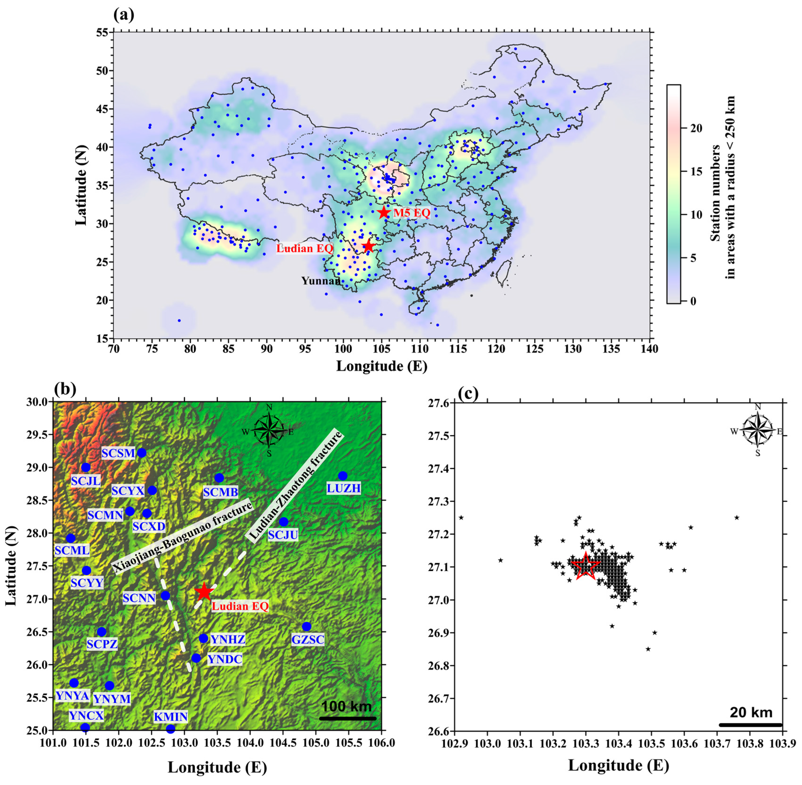
The Ludian earthquake (103.4°E, 27.2°N) with the moment magnitude (Mw) of 6.1 occurred in China on 3 August 2014 (Figure 1). The data of a cGNSS array of about 300 stations covering an area of approximately 3500 × 3000 km² is analyzed with the HHT in order to study the temporal evolution of the non-linear, non-stationary earthquake-induced signals related to the stress accumulation, and thus the potential earthquake preparation zone of the event. Note that the 260 cGNSS station used in this study are installed by China Earthquake Administration and they also belong to the Crustal Movement Observation Network of China (CMONOC). The rest of the stations located at surrounding Mainland China are retrieved from Nepal continuous GPS network and IGS networks.

In this study, we calculated surface deformation within a time span from 2012 to 2015. The surface deformation of the stations near the epicenter was compared to the distant ones by calculating the cross coefficient in order to quantify the abnormal variations. The HHT was used to filter out the long-term secular tectonic movement, the seasonal (including annual and semi-annual) and the short-term noise from the time series. As a result, the behavior of crust deformation in the terminal stages of failure can be revealed. In addition, the orientations of the frequency-dependent deformed vectors were compared to the most compressive axis of the Ludian earthquake derived from the Global CMT project to confirm that the retrieved signals are seismogenic due to the stress accumulation in the crust. The temporal evolution of the frequency-dependent deformation can be examined to explain the unusual distribution of the aftershocks and to determine the size of the earthquake preparation zone.

2. Materials and Methods

In order to efficiently retrieve the seismo-deformation signals shortly before an earthquake, an empirical relationship describing the terminal stage of failure under the condition of constant stress and temperature [16,17] is employed. This relationship is related to the general constitutive laws in damage-mechanics models [18]. The empirical relationship is expressed as

$${\dot{\mathsf{\Omega }}}^{-\alpha }\stackrel{\dot{}\dot{}}{\mathsf{\Omega }}-A=0,$$

(1)

where Ω is an observation (e.g., strain or displacement) and A and α are empirical constants. The dots denote the time derivatives. When α is close to 2, it implies that the acceleration changes in Ω is approaching the terminal stage. This empirical relationship provides a useful description of creep and deformation before landslides and volcanic eruptions [19] and it is related to the general constitutive laws used commonly in damage-mechanics models [18]. Stress accumulates in the crust and gradually approaches the threshold of fault rupture shortly before an earthquake. The process is related to the terminal stage of failure and thus, the quantity represented by Ω can be strain or displacement of rocks or soils.

In order to retrieve the acceleration changes of crustal deformation in the terminal stage of the fault failure, data of about 300 cGNSS stations in continental China well covering the areas around the Ludian earthquake was collected. We processed the daily solution of these stations using GAMIT/GLOBK software with a 24-hour ionosphere-free combination to fix the ambiguities. We adopted the precise orbits from the International GNSS Service for Geodynamics (IGS), the precise EOPs from the IERS Bulletin B, and the IGS tables for phase center of the antennae. We estimated one tropospheric zenith delay and two horizontal gradients of that at each station every 2 hours each day. The resulting daily solutions are stacked and loosely constrained in the International Terrestrial Reference Frame (ITRF2008) to a set of global stable stations released by the Scripps Orbital and Permanent Array Center [20].

Earthquake-related acceleration changes in the temporal domain is generally parabolic, which is non-linear. To examine the existence of the empirical relationship in crustal deformation before earthquakes, a linear trend is removed from the daily solutions of the cGNSS data to enhance the acceleration changes. The acceleration changes can be observed from the daily solutions of the cGNSS data once a linear trend is removed. The following processes are utilized to retrieve the acceleration changes for further examining the relationship between the acceleration changes and earthquakes parameter. Note that the acceleration changes are non-stationary due to the mature of the discontinuous occurrence of an earthquake. The HHT is suitable in this case since it preserves the non-linearity of the time series. It is utilized in this study to extract the non-linear and non-stationary features in the cGNSS time series. However, the parabolic variation of an acceleration change is not frequency-dependent, so it covers a very wide band in the frequency domain. To overcome this, a band-pass filter of 20–150 days was employed to retrieve the acceleration changes from the cGNSS time series [21].

The HHT comprises two major processes: the Empirical Mode Decomposition (EMD) and the Hilbert-transform (HT). The EMD process decomposes time series into many Intrinsic Mode Functions (IMFs) and a residual based on the characteristics of signal energy. The residual is generally considered to be the long-term trend of the time series with no significant frequency characteristics, while each IMF is considered as the instantaneous frequency and amplitude at each observed epoch. When using HHT to study the crustal deformation, the residual is the long-term plate tectonic movements [22,23], whereas the IMFs are the frequency-dependent components which represent the nature of the deformation with the long-term tectonic movements removed. The “filtered GNSS data” hereafter denotes the observed cGNSS deformation time series with the residual (the long-term tectonic movements) and the frequency-dependent IMFs (the frequency-dependent factors common to all stations such as annual, semi-annual and seasonal variations and noise) removed. It reveals the abnormal acceleration changes approaching the terminal stage. Notably, the processes regarding the removal of the residual and the frequency-dependent components can be simplified by using a band-pass filter of 20–150 days via HHT in the frequency domain [21].

The orientations of the filtered GNSS data, or the “GNSS-azimuth” thereafter, are further computed. In general, the GNSS-azimuth of all stations in an area exhibits random-like disordering due to the removal of the long-term tectonic movements, so one cannot find a definite common orientation for all stations. At this point, the abnormal acceleration change is insignificant. When the earthquake-related stress accumulates, as the crust gradually approaches the terminal stage of material failure, the abnormal acceleration change starts to dominate and the disordered GNSS-azimuth of stations starts to align to a common direction, indicating the existence and the influence of the accumulated stress. The alignment becomes disordered once again when the earthquake preparation is finished at the terminal stage.

3. Results

Figure 2, Figure 3 and Figure 4 are the NS, EW and vertical components of the GNSS data at the stations (listed in

Table 1. The latitude and longitude of the cGNSS stations with 2.5° to the epicenter.

Station (code)	Latitude (N)	Longitude (E)
YNCX	25.05	101.49
LUZH	28.87	105.41
SCJL	29.01	101.50
SCSM	29.23	102.35
YNYA	25.72	101.33
KMIN	25.03	102.80
SCML	27.93	101.28
YNYM	25.69	101.86
SCMB	28.84	103.53
SCYX	28.65	102.51
SCYY	27.43	101.51
SCMN	28.33	102.17
SCPZ	26.50	101.74
SCJU	28.18	104.52
SCXD	28.30	102.44
YNDC	26.11	103.18
YNHZ	26.41	103.29
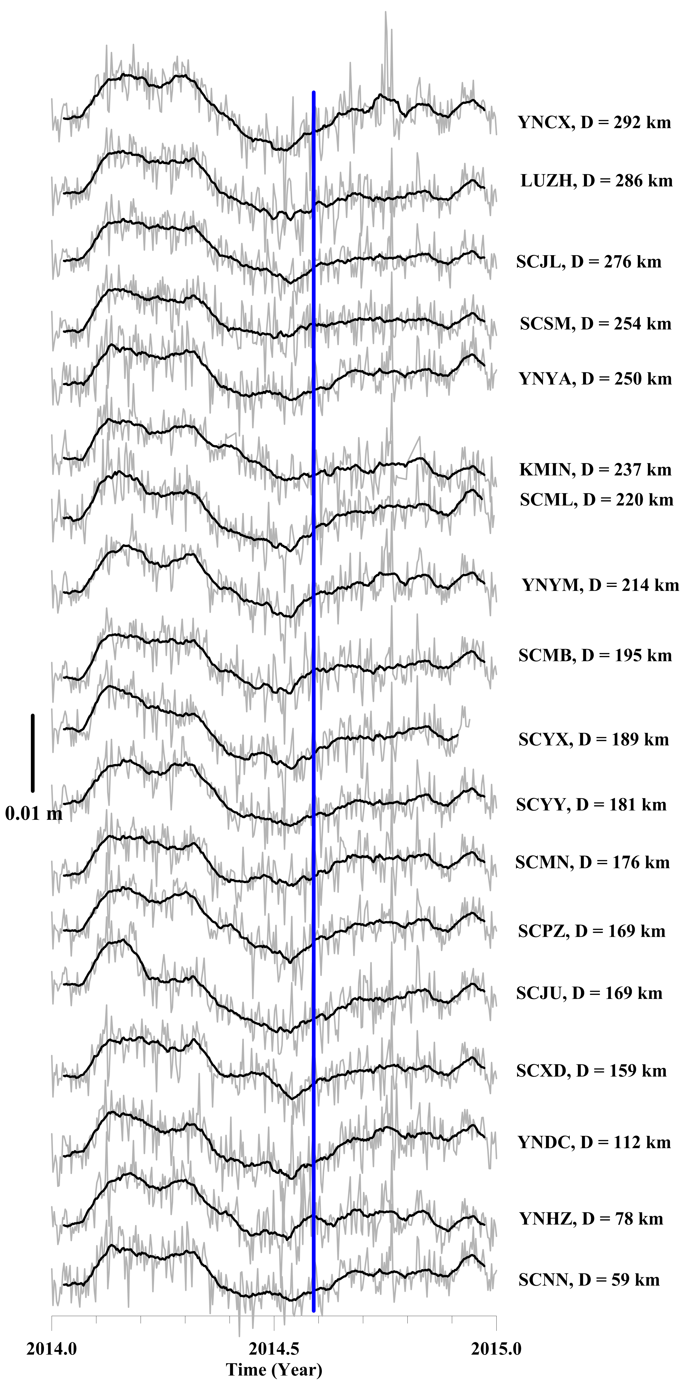
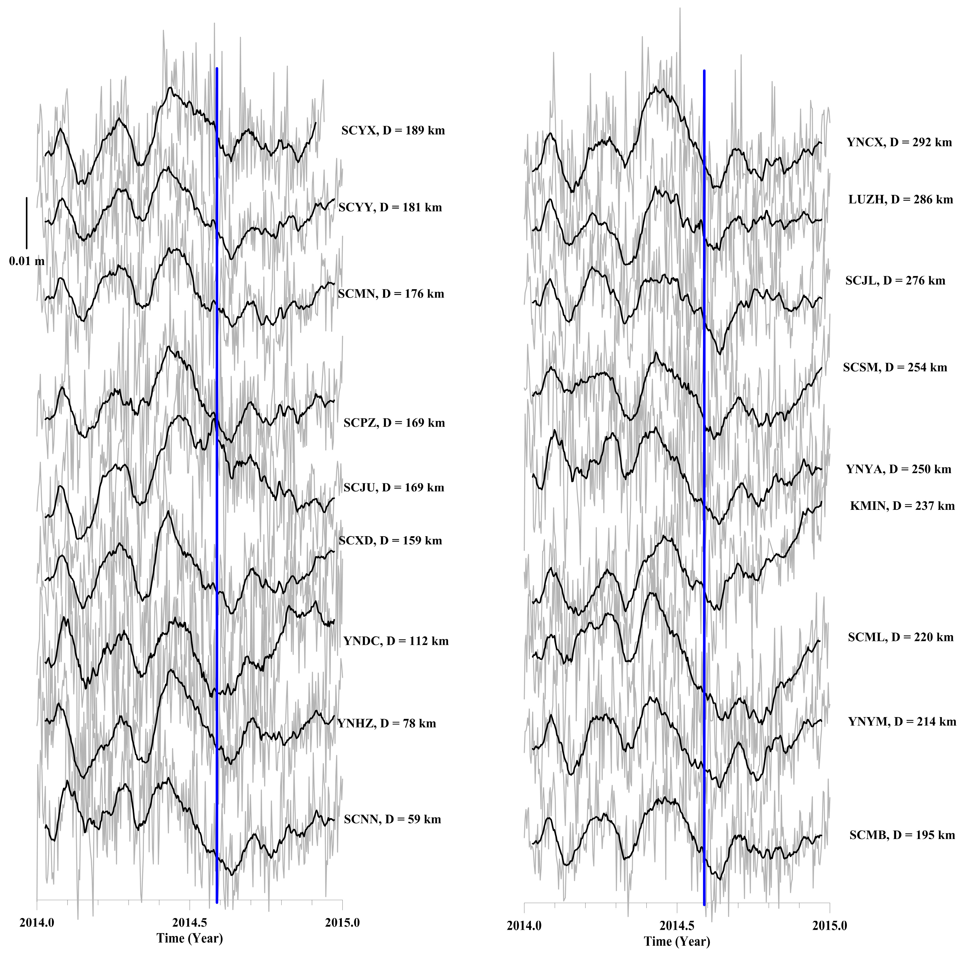
SCNN	27.06	102.72

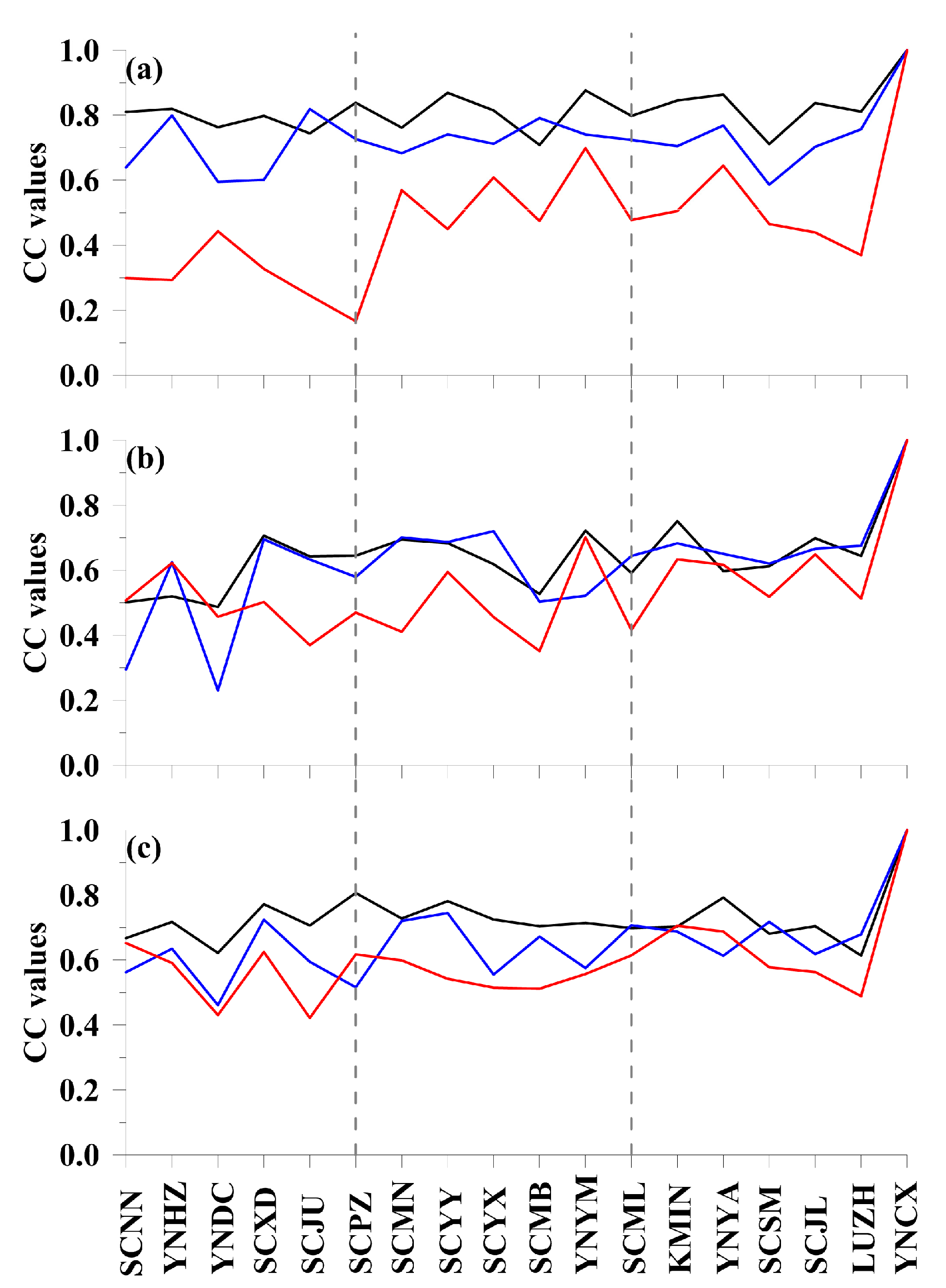
) within 2.5° from the epicenter after the removal of a linear trend with the empirical relationship (1) to examine the existence of the acceleration changes. The data in the NS component (Figure 2) shows an acceleration change toward the north in most of the stations during 2014.15–2014.32 due to unknown factors. Variations of the data became smooth after 2014.32, except for abnormal short-term event at about 2014.5. This short-term event is an unusual increase at 2014.48 and an abnormal decrease at 2014.5 at most stations 200 km within the epicenter. To quantify the difference between the data during the short-term event, the cross correlation (CC) methods were utilized. YNCX was selected as the reference and the CC values were computed using two reference windows of 2013.45–2013.58 (i.e., 366–415 days before the EQ) and 2014.31–2014.44 (51–100 days before the EQ) and additionally, one monitoring window of 2014.45–2014.58 (1–50 days before the EQ) was selected. As can be seen in Figure 5a, the CC values derived from the two reference windows are mainly inversely proportional to the epicentral distance. The correlations of station pairs in these two windows are between 0.7–0.8. This implies that the data are highly correlated at the station pairs during these 2 reference windows. In contrast, the correlation derived from the monitoring window, 1–50 days before the Ludian earthquake, is generally smaller than 0.6. The significantly smaller CC values suggest that the GNSS data after the removal of a linear trend are potentially affected by the earthquake-related stress 50 days before the mainshock.

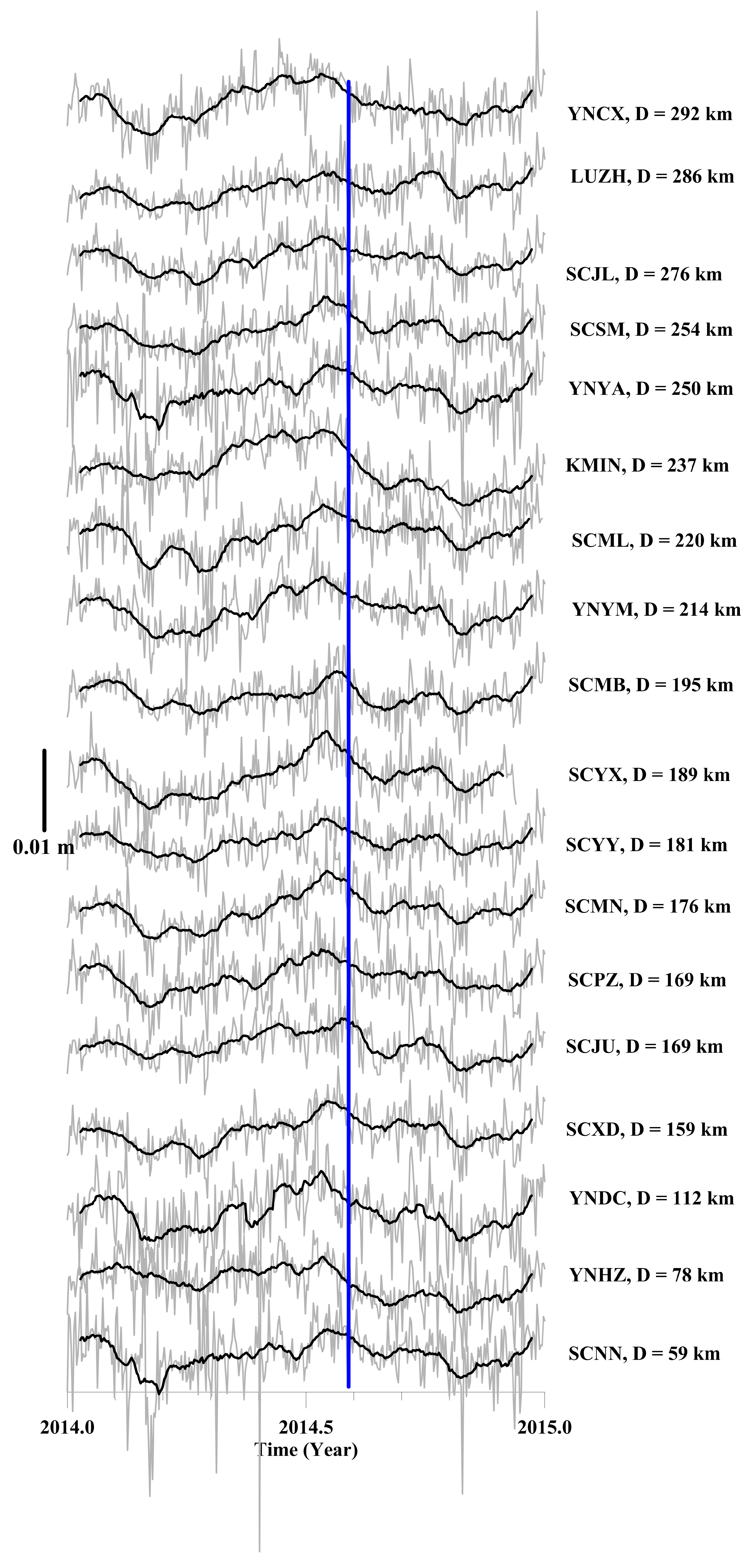
Regarding the EW component, a few periodic vibrating cycles (with an amplitude of 0.005 m and a duration of approximately 40 days) can be found during 2014.0–2014.5. A significant eastward acceleration changes were observed at most stations from 2014.15 to 2014.58, though the highest peak at each station does not appear at the same time. Sharp inverse changes were observed at YNHZ, YNDC, SCYX, YNYM, SCML and SCSM. The time-shift anomalies appeared on the data at the SCXD, SCPZ, SCJU and SCMB stations. A step was observed at the YNDC station before the Ludian earthquake. Nevertheless, the general trend of the abnormal changes can be observed from the data at the most stations 200 km within the epicenter. The CC values of the data in the EW component are mainly between 0.5 and 0.7 (Figure 5b). These smaller CC values suggest that the variations of the data in those station pairs are partially independent. When we consider the results derived from the monitoring windows (i.e., 1–50 days before the mainshock), the CC values are similar to those stations with the epicentral distance either less than 169 km or larger than 200 km. Regarding the CC values obtained from the data recorded by the station with the epicenter distance between 169 km and 200 km, a significant drop of about -0.15 can be found. This suggests that the earthquake-related stress affected the cGNSS data of the EW component and thus reduced their correlation.

Larger fluctuations (approximately 0.01–0.02 m) in the vertical component can be found a few months before the earthquake (Figure 4). The vertical component of each stations generally shows in-phase variation at most stations. Three obvious cycles can be found from 2014.0 to 2014.58. The significant abnormal changes with an amplitude of about 0.02 m can be found at the SCJU station, which is located 169 km away from the epicenter of the Ludian earthquake. The abnormal changes with relatively-small amplitude can also be observed from the data at most stations. In terms of the CC values examined via the two reference windows in Figure 5c, the values are between 0.5 and 0.8. No significant difference was found from the values derived from the reference and monitoring windows. The smaller correlation (about 0.05 less) could be caused by either the temporal window or artificial noise. Thus, the cGNSS data on the vertical component are not utilized in the following analysis, only the horizontal ones are analyzed further. In short, the acceleration changes can be found from the cGNSS data after the removal of a linear trend. The relative-small CC values suggest the existence of crustal deformation close to the epicenter several days before the occurrence of the Ludian earthquake, particularly on the NS and EW components of the cGNSS data. However, the acceleration changes are not unusual and can be frequently found from the cGNSS data. The anomalous deformation is very difficult to be directly retrieved from the daily solutions (Figure 2, Figure 3 and Figure 4).

Here, we take the GNSS data on the NS and EW components at the SCNN station as an example to illustrate the removal of the unwanted influences (i.e., the short-term noise, semi-annual and annual variations and long-term plate movements) using a band-pass filter of 20–150 days via HHT (also see Chen et al., 2020 [24]) to further examine the relationship between the acceleration changes and parameters of earthquakes. 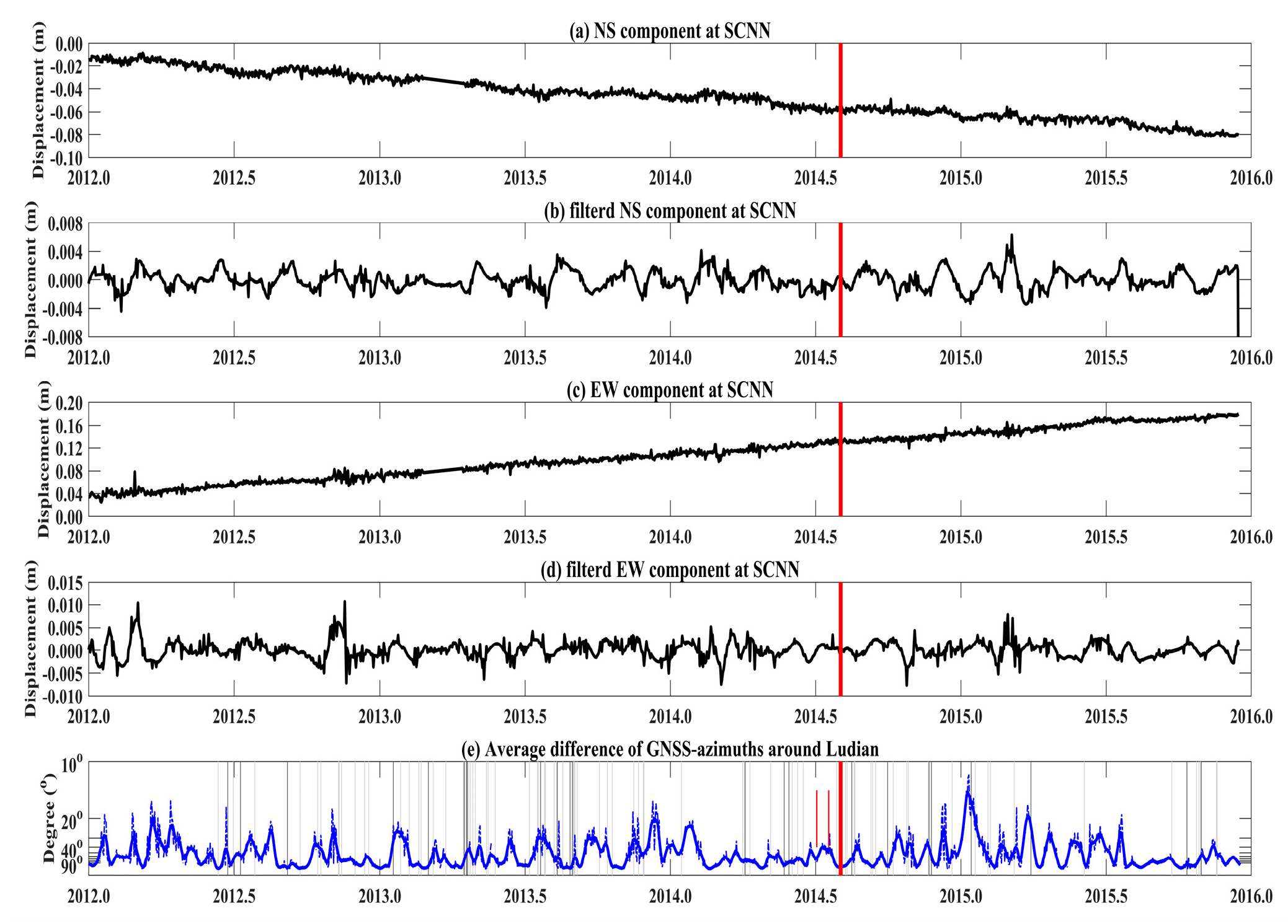Figure 6a,c present the NS and EW components of the daily solution at the SCNN station from 2012 to 2015. Significant semi-annual variations along with a long-term southward trend can be found on the NS component in Figure 6a. In contrast, annual variations along with a long-term eastward trend can be observed on the EW component in Figure 6c. When these data are filtered with HHT, the unwanted influences are clearly removed from the filtered GNSS data (Figure 6b,d). Note that the amplitude of the filtered data on the NS and EW component is about 8 mm and 10 mm during 2012–2015, respectively. The NS and EW components of the filtered data are further utilized to compute the GNSS-azimuth to understand the seismo-deformation associated with the Ludian earthquake. We computed the average difference of the GNSS-azimuths around the Ludian area by using every two stations located within the epicentral distance < 300 km, (i.e., the 18 stations listed in Table 1) during 2012–2015 (Figure 6e). The larger average GNSS-azimuth difference implies that the orientation of the anomaly at these 18 stations are not common, that is more disordered, whereas the smaller difference indicates they are roughly aligned to a general azimuth. We focused on the changes of the average difference before the occurrence of the Ludian earthquake. The difference is about 90° 30 days before the Ludian earthquake and gradually decreases to 30° 15 days before the event. Then, the difference increases again a few days before the Ludian earthquake. The entire temporal evolution of the average GNSS-azimuth forms a unique disorder-alignment-disorder sequence before the Ludian earthquake. Not only can be seen in the Ludian earthquake, this unique disorder-alignment-disorder sequence can also be found in other events around the Ludian area (Figure 6e). The unique sequence observed in this study also agrees with the observation in the previous studies [21,22,23,24]. However, earthquake occurrence does not follow the sequence and no event is detected after the sequence that can be found during the study period.

To examine whether the aligned GNSS-azimuths are useful crustal displacement information before earthquakes around the Ludian area, statistical tests of the Molchan’s error diagram is performed in this study. The Molchan’s error diagram is a conventional method to evaluate the prediction performance of given observations for earthquake forecasting. It shows the rate of earthquakes successfully detected against the rate of alarmed cells [25,26]. Figure 7a shows the Molchan’s error diagram of the optimal prediction strategy based on the average difference of the GNSS-azimuths related to earthquakes with magnitude ≥ 5 around the Ludian area during 2012–2015. The prediction curve (the bold red line) is obviously over the random prediction line (i.e., the black diagonal line). Most perdition curve are comparable with the 90% confidence interval, and quite a few even exceed the 95% confidence interval. Considering the earthquakes with magnitude ≥ 5.5 during the same temporal period, the prediction curve is generally over the 95% confidence interval (Figure 7b). Meanwhile, a great result with the alarm rate of ~0.35 and the detection rate of ~0.72 can be obtained that is significantly larger than 95% confidence interval. These results suggest that the aligned GNSS-azimuths used in this study provide useful crustal displacement information before earthquakes and are beneficial to earthquakes when predicting earthquakes with relatively larger magnitude.

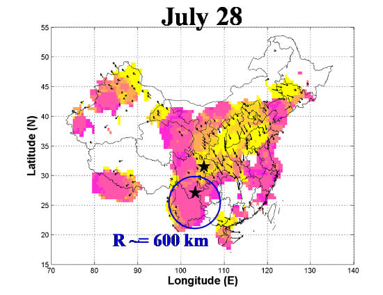
Figure 8 reveals the GNSS-azimuth distribution from July 5 to August 2 in 2014 associated with the Ludian earthquake. No aligned GNSS-azimuths in a large scale can be found on 5 July 2014 (i.e., 29 days before the Ludian earthquake) because the long-term plate tectonic movements have been removed. Those disordered GNSS-azimuths were gradually turned to a common direction toward the southeast and this can be seen in the inset for 9 July 2014 in Figure 8. Two circle-like regions located at (30°N, 107°E) and (25°N, 100°E) are surrounded by the aligned GNSS-azimuths on 18 July 2014. The phenomenon of surroundings became clear for the region (25°N, 100°E) on 23 July 2014. Areas with aligning GNSS-azimuths gradually decreased on 20 July 2014. Notably, disordered GNSS-azimuths regions remain at the epicenters of the M5 earthquake (31.45°N, 105.30°E) on 29 July 2014 and the Ludian (27.2°N, 103.4°E) earthquake on 3 August 2014. After the occurrence of the M5 earthquake, the increase of disordered regions reached to the maximum on 2 August and the Ludian earthquake occurred one day thereafter. The analytical results suggest that non-linear abnormal changes in the cGNSS data shown in Figure 2, Figure 3 and Figure 4 can be effectively retrieved by using the HHT. The disorder-alignment-disorder sequence shown in Figure 6e can be repeatedly observed in the spatial domain in Figure 8. Meanwhile, the sequence (Figure 6e and Figure 8) agrees with the observations of earthquakes in Japan and the Taiwan region [21,22,23,24].

4. Discussion

Changes in physical parameters during an earthquake are commonly divided into four stages: Buildup of elastic strain, dilatancy and crack development, unstable deformation in the fault zone, and a sudden stress drop followed by mainshocks [17]. For a strike-slip fault, straight lines can be easily identified across both sides of a fault and they remain parallel in the first stage of elastic strain buildup. In the stage of dilatancy and crack development, these lines are bent when the stress continues to accumulate in the crust forming a locked region somewhere in the focal area. The bending temporally stops due to the unstable deformation triggered by the accumulated stress when it approaches the terminal stage of the fault rupture. After the mainshock, the accumulated stress rapidly drops. We noticed that there are disordered GNSS-azimuths retrieved from the filtered GNSS data 29 days (i.e., July 5) before the Ludian earthquake, suggesting that the earthquake-related stress is in the first stage of elastic strain buildup. Then, during the period of 25–11 days before the Ludian earthquake (i.e., July 9–23), the stress accumulation continues and cracks start to develop causing the dilatancy of the crust, so the disordered GNSS-azimuths become aligning to a certain common direction. The most compressive axis of the M5 earthquake and the Ludian earthquake is about 187° and 295°, respectively, which are computed by using the standard method [27]. Interestingly, the alignment of the GNSS-azimuths with orientations was ranging about 170°–180° and 270°–330°, 2 days before the M5 and the Ludian earthquake, respectively. This finding matches surprisingly well with the direction of the most compressive axis of these two earthquakes. The stress dominates the deformation with the NS and the EW orientations in the earthquake-related areas that could reasonably cause the aftershocks to distribute in the NS and EW directions, simultaneously (Figure 1c). Regarding the third stage, there’s no significant ground uplifts and tilts observed in the area from July 18–27 for the M5 earthquake and July 20–August 2 for the Ludian earthquake. This agrees with the disordered GNSS-azimuth we found in the same periods. This is about 1–5 days before the earthquake (i.e., July 30–August 2) and is the stage when the abnormal changes in strainmeters, groundwater level, water temperature and radon concentration started to be noticed and reported [28]. In summary, the development of the disorder-alignment-disorder sequence we found in the GNSS-azimuth agrees with the four stages of seismo-deformation of an earthquake.

Studies have suggested that the crustal deformation can originate from atmospheric pressure during typhoons and heavy rainfall [29]. We retrieved the time series of the NS and EW displacements at the KUNM station, which is the closest one (about 250 km) to the Ludian area in the Global Geophysical Fluids (GGFC) Service of IERS [30], to clarify the induced atmospheric pressure and water mass loadings. The induced atmospheric pressure and water mass loadings are mainly in the ranged between -0.5 mm and 0.5 mm at the KUNM station that is significant smaller than the amplitude of ~8 mm for the NS and ~10 mm for the EW component of the filtered GNSS data at the SCNN station (Figure 6b,d). In addition, based on [29], when atmospheric pressure decreases 50 HPa, a volumetric strain increases about 100 nanostrain, that is 1 mm over 10 km, at the typhoon center as verified by borehole strainmeter in Taiwan. Typhoon Rammasun was formed on the Pacific Ocean on July 11 and disappeared in Yunnan, China on July 20 in 2014. The minimum distance between the epicenter and the typhoon is about 450 km on July 20 while the atmospheric pressure at the typhoon center is reported as 998 HPa [31]. Considering the normal atmospheric pressure of 1,013 HPa, the atmospheric pressure drops 15 HPa, which roughly corresponds to 30 volumetric nanostrain at the typhoon center according to [29]. Considering the epicenter of Ludian Earthquake is 450 km away from the typhoon center with much smaller atmospheric pressure change, the possible effect on the crustal deformation caused by atmospheric pressure change would be negligible and mostly in the vertical. However, the GNSS-azimuths were calculated with horizontal components. In addition, the effect of atmospheric pressure change is almost immediate as mention above, but the seismo-deformation we detected lasts longer. On the other hand, Zeng et al. (2015) [28] reported that the rainfall around the Ludian area is mainly concentrated on July 13–16. However, the aligned GNSS-azimuths in a large area can be observed on July 18. The increase of disordered regions associated with the Ludian earthquake is mainly from July 9 to August 2 which does not correspond to the rainfall. In short, the temporal discrepancy suggests that the seismo-deformation observed in the study is unlikely to be resulted from the typhoon or the rainfall.

A strong spatial correlation among GNSS stations of a network results in a common position movement (a few mm) of nearly entire network. It is called the common-mode error (CME). A regional filter or a stacke-and-remove procedure are the common mitigations [1,3]. The CME is revealed by the apparent seasonal (annual and semiannual) variation, ~40% of whose power can be explained by contributions of mass redistribution [32]. Its causes are still unclear, but the consensus is that they are related to the changes in environmental mass redistribution, including atmospheric loading, continental water-storage loading, and non-tidal ocean loading [2,7,8]. Other potential candidates include thermal expansion of monuments [32,33], mis-modeling in orbits, antenna phase centers, reference frames, EOP (Earth Orientation Parameters), and systematic errors due to the choice of processing centers [9]. A close look with GNSS stations in the North American and Pacific plates suggests that the cross correlation among GNSS stations within 1000 km is 0.95 and it goes to 0 gradually as the distance increases and reaches 6,000 km [4]. The CC values are comparable regardless of the epicentral distance during the normal time (i.e., 366–415 days and 51–100 days before the Ludian earthquake) and are inversely proportional to the epicentral distance at 1–50 days before the earthquake (Figure 5). This implies that the low CC values are not dominated by the CME but earthquake-related stress changes. Notably, the alignments of the GNSS-azimuths distribution areas exceed 500 km in radius (see the distribution on July 18–23 in Figure 8). The agreement between the orientation of GNSS-azimuths and the most compressive axis of the earthquake suggests that the earthquake-related stress accumulation and the CME should be further examined and separated. The stressed areas triggering fault dislocation before earthquakes observed in this study are significantly larger than the post seismic crustal deformation. We compared the size of stressed areas to the earthquake preparation zones estimated using numerical models and seismicity [34,35,36,37]. The size of the earthquake preparation can be approximated by the formula of R = 100.43M, where R is the radius of the earthquake preparation and M the magnitude of earthquakes. Accordingly, the radii of the earthquake preparation are 141 km for the M5 earthquake and 420 km for the Ludian earthquake, respectively. The unique phenomena of disordered regions surrounded by the aligned areas could indicate a locked fault as the developments of an upcoming earthquake approaches the terminal stage or the critical stage. The regions with a radius of about 250 km and 600 km can be clearly identified a few days before these two earthquakes (i.e., the terminal stage) and this in general agrees with the radius of the earthquake preparation zone proposed in [35]. Further studies are required in the future to compare the observed locked zone in the critical stage to a potential earthquake preparation zone.

5. Conclusions

In this study, we found that the crustal deformation exhibits a disorder-alignment-disorder sequence of the GNSS-azimuths days before the Ludian earthquake in China. The sequence is similar to the observation of the seismo-deformation anomaly two months before the Tohoku-Oki earthquakes in Japan [23] and tens of days before several earthquakes in the Taiwan region [21,22,24]. An agreement between the orientations of the GNSS-azimuths and the direction of the maximum compressive axis of the two earthquakes suggests that the alignment is seismogenic. Thus, the sequence could be utilized to identify crustal seismo-deformation signals in the terminal stage of material failure of earthquakes in distinct areas of the world. The disordered region surrounded by the aligned areas implies the general area of the locked zone, which is apparently approaching the terminal stage of an earthquake. Compared to what we have done in Japan and the Taiwan region, the full picture of the sequence of the GNSS-azimuth cannot be clearly observed there due to the limitation of the land area. However, with a wider coverage of cGNSS stations in China, we can observe the full picture of this sequence, both in the spatial and temporal sense, in this study. Meanwhile, the size of the locked zone roughly supported by an earthquake preparation zone calculated by numerical models [35]. The finding of the disordered regions would be useful when one attempts to separate the earthquake-related stress from the cGNSS common-mode error. However, this requires further investigation and is beyond the scope of this study.

The observation of seismo-deformation signals can also be a candidate of a promising anomalous phenomenon. This sheds light on the estimation of earthquake-related stress accumulation in the crust via strain changes in the terminal stage. The estimation is beneficial in understanding groundwater variations, underlying velocity and electrical conductivity. This valuable information is potentially helpful in developing physical mechanisms with distinct physical parameters. Once the physical mechanisms can be supported by distinct physical parameters, it is anticipated that the sesimo-anomalies could become reliable and available.