Ice Concentration Retrieval from the Analysis of Microwaves: A New Methodology Designed for the Copernicus Imaging Microwave Radiometer

Abstract

Over the last 25 years, the Arctic sea ice has seen its extent decline dramatically. Passive microwave observations, with their ability to penetrate clouds and their independency to sunlight, have been used to provide sea ice concentration (SIC) measurements since the 1970s. The Copernicus Imaging Microwave Radiometer (CIMR) is a high priority candidate mission within the European Copernicus Expansion program, with a special focus on the observation of the polar regions. It will observe at 6.9 and 10.65 GHz with 15 km spatial resolution, and at 18.7 and 36.5 GHz with 5 km spatial resolution. SIC algorithms are based on empirical methods, using the difference in radiometric signatures between the ocean and sea ice. Up to now, the existing algorithms have been limited in the number of channels they use. In this study, we proposed a new SIC algorithm called Ice Concentration REtrieval from the Analysis of Microwaves (IceCREAM). It can accommodate a large range of channels, and it is based on the optimal estimation. Linear relationships between the satellite measurements and the SIC are derived from the Round Robin Data Package of the sea ice Climate Change Initiative. The 6 and 10 GHz channels are very sensitive to the sea ice presence, whereas the 18 and 36 GHz channels have a better spatial resolution. A data fusion method is proposed to combine these two estimations. Therefore, IceCREAM will provide SIC estimates with the good accuracy of the 6+10GHz combination, and the high spatial resolution of the 18+36GHz combination.

1. Introduction

Over the last 25 years, the increase in Arctic air temperature has been twice as high as anywhere else on the planet, resulting in dramatic changes in these areas [1]. The extent and thickness of Arctic sea ice have declined, especially during summer. Coupled regional/global climate models still fail to replicate this decline: they underestimate the observed reduction in sea ice, showing that physical processes and feedback mechanisms are not yet well represented [2,3]. The so-called Arctic amplification has repercussions on the low latitudes, but the prediction of these models is still inadequate [4,5,6].

Since the 1970s, passive microwave imagers have provided an estimate of sea ice concentration [7] and it is one of the longest satellite climate series. The microwave data between 6 and 37 GHz are less affected by clouds than the visible and infrared observations and do not depend on sunlight. However, the quality of the sea ice concentration estimates is still limited, mainly because of the spatial resolution of the instruments. Microwave low frequencies (<11 GHz) are hardly affected by the atmosphere and allow for a good accuracy of the estimate, but provide limited spatial resolution. Microwave higher frequencies (>30 GHz) have better spatial resolution, but are more affected by atmospheric disturbances and they are less sensitive to the sea ice signal. The algorithms for sea ice characterization are not currently optimized to jointly exploit the radiometric sensitivity of the low frequencies and the spatial resolution of the high frequencies.

A new mission is currently under study for the next generation of Copernicus satellites. The Copernicus Imaging Microwave Radiometer (CIMR) is a high priority candidate mission within the European Copernicus Expansion program, with a special focus on the observation of the polar regions. It is a conically scanning microwave radiometer imager that includes channels at 1.4, 6.9, 10.65, 18.7, and 36.5 GHz (all with both vertical and horizontal polarizations), in a sun-synchronous polar orbit, to provide as primary variables the Sea Ice Concentration (SIC) and Sea Surface Temperature (SST). It will follow the current missions (Advanced Microwave Scanning Radiometer 2 (AMSR2), Soil Moisture Ocean Salinity (SMOS) or Soil Moisture Active Passive (SMAP)) whose continuity is not currently guaranteed. CIMR will provide increased accuracy and/or spatial resolution compared to the current missions, thanks to its low noise receivers, and its large deployable mesh antenna of ∼7 m in diameter (see

Table 1. Passive microwave radiometer spatial resolutions.

Frequency	Spatial Resolution (km)
(GHz)	CIMR	AMSR2
6.9	15	48
10.6	15	33
18.7	5	18
36.5	5	9

). This is an opportunity to develop new algorithms for SIC, that will benefit the upcoming CIMR instrument but also the current AMSR2 mission.

Generally, a radiative transfer model is used for the inversion of satellite Brightness Temperatures (TBs) to retrieve geophysical variables. In the case of sea ice, radiative transfer models are still in the development phase: the emission processes in sea ice are complex and depend on a large range of microphysical variables [8,9] that are not available in the retrieval process. Forward simulation of the sea ice emission is still challenging. Current SIC algorithms rely instead on empirical methods, using the difference in radiometric signatures between the open ocean and the sea ice, based on the fact that the ocean emissivity is significantly lower than the sea ice emissivity. Many efficient SIC retrieval algorithms have been developed and are applied operationally. The NASA/TEAM algorithm [10,11], the Bootstrap algorithm [12] and the Bristol algorithm [13] are popular. More recent algorithms use combinations of these methods, with some adjustments, like the Ocean and Sea Ice-Satellite Application Facility (OSI-SAF) algorithm supported by EUMETSAT [14,15]. These algorithms use a limited number of channels to estimate the SIC. Most of them are based on channels at 18 and 36 GHz. An evaluation of an ensemble of SIC algorithms showed that the algorithm using 6.9 GHz observations had the lowest error [16], because that frequency is less affected by the atmosphere and by the snow cover than the higher frequencies. However, the spatial resolution at 6.9 GHz, with current and past missions, is very coarse compared to higher frequencies. Table 1 presents the spatial resolution of the CIMR channels, as compared to the AMSR2 mission (the table is limited here to their common frequencies, that are of interest here for SIC retrieval).

Here, we proposed a new methodology called Ice Concentration REtrieval from the Analysis of Microwaves (IceCREAM) algorithm. This method can accommodate a large range of channels, from the low microwave frequencies (6 and 10 GHz) that are more sensitive to the sea ice presence, to the higher frequencies (18 and 36 GHz) that can provide good spatial resolution. The retrieval will combine the sensitivity of the low frequency channels with the good spatial resolution of the high frequencies. It will be based on an optimal estimation scheme [17], adapted to SIC retrieval. A simple linear model will link the satellite measurement to the SIC, derived from a large collection of satellite microwave observations for 0% and 100% SIC. A method will be proposed to efficiently merge the full range of frequencies, to produce a final SIC at the spatial resolution of the high frequencies. Great care will be exercised to quantify both the systematic and random errors resulting from the new algorithm.

Section 2.1 will describe the optimal estimation methodology, adapted to the SIC retrieval. The database of passive microwave observations at 0% and 100% SIC will be presented (Section 2.2). In Section 3, the sensitivity of the retrieval to the hypotheses will be analyzed. In Section 4, a data fusion method will be presented to improve the SIC estimations at high spatial resolution. Section 5 will conclude this study.

2. Method

2.1. An Optimal Estimation Scheme

A new methodology is adopted to estimate the SIC. It is based on the classical optimal estimation scheme [17,18] that is largely adopted for the estimation of ocean and atmospheric parameters. It uses the derivative of the observations with respect to the parameter to retrieve (also called the Jacobian and usually calculated from a radiative transfer forward model), as well as the observation error, the forward model error, and an a priori estimate with its associated error. It can be expressed as follows:

$$x_{i+1}=x_i+Q(K^t{S}_e^{-1}(y-F\left(x_i\right))+S_a^{-1}(x_i-x_a))$$

(1)

x is the parameter to retrieve, y the satellite observations, $F\left(x\right)$ represents the forward model, K the Jacobian matrix, $S_e$ is the observation error covariance matrix, $x_a$ the a priori information on x, $S_a$ the a priori error covariance matrix, and i the iteration step. To start the iteration process ($i=0$), a first guess value $x_0$ is needed, it can be the same as the a priori value. The covariance matrix of the retrieval error Q is expressed as:

$$Q={(K^t{S}_e^{-1}K+S_a^{-1})}^{-1}$$

(2)

The square root of the diagonal element of the Q matrix gives the theoretical retrieval error.

In our case, the only variable x to retrieve is the SIC, and the vector y represents the TBs observed at different frequencies. As we retrieve only one parameter x, Q, $x_a$ and $S_a$ are scalar. In this formalism, y, K, and $F\left(x\right)$ are matrix of dimension $1\times N_{channels}$ and $S_e$ is a matrix of dimension $N_{channels}\times N_{channels}$, where $N_{channels}$ is the number of radiometric channels used for the retrieval. This method was already briefly introduced for SIC retrieval in Kilic et al. [19].

For the inversion a forward model $F\left(x\right)$ is needed. In the case of SIC, there is no radiative transfer model to efficiently relate the TBs to the SIC. The forward model is empirically based on the contrast between ocean and ice TBs. The mean TBs for the open ocean (${\mathrm{TB}}_{ocean}$, corresponding to 0% SIC also noted SIC0) and for the total ice cover (${\mathrm{TB}}_{ice}$, corresponding to 100% SIC also noted SIC1) are estimated from a collection of passive microwave observations. They are called the tie points. Then, the forward model is a linear mixing model derived from the TB contribution of the two extreme surface types (SIC0 and SIC1) within the sensor footprint. It can be expressed as:

$$TB=F\left(SIC\right)=SIC·T{B}_{ice}+(1-SIC)·T{B}_{ocean}$$

(3)

The Jacobian matrix K contains along its column the derivative of the TB as a function of the SIC for the different channels. For a given channel:

$$K_{channel}=\frac{\partial T{B}_{channel}}{\partial SIC}=T{B}_{ice,channel}-T{B}_{ocean,channel}.$$

(4)

The observation error matrix $S_e$ is expressed as:

$$S_e=SI{C}^2·CO{V}_{T{B}_{ice}}+{(1-SIC)}^2·CO{V}_{T{B}_{ocean}}.$$

(5)

$CO{V}_{T{B}_{ocean}}$ and $CO{V}_{T{B}_{ice}}$ are the error covariance matrices of the extreme cases, i.e., the open ocean (SIC0) and the total ice cover (SIC1). A proxy of this information is the covariance of the ${\mathrm{TB}}_{ice}$ and ${\mathrm{TB}}_{ocean}$ for the considered frequencies, in the collection of passive microwave observations at SIC0 and SIC1. The instrument noise is neglected as it is small compared to the observation error specifications $CO{V}_{T{B}_{ocean}}$ and $CO{V}_{T{B}_{ice}}$.

In the following, the a priori SIC value ($x_a$) is taken at 50%, along with a covariance error $S_a$ of 25%. The inversion is initialized with a first guess $x_0$ equal to the a priori $x_a$. Only two iterations are done as the problem is linear. The second iteration is required to update the retrieval error value, but it does not change the SIC value found at the first iteration.

2.2. The Round Robin Data Package

The Round Robin Data Package (RRDP) [20] has been developed for the European Space Agency (ESA) sea ice Climate Change Initiative (CCI) project. It is openly available (https://figshare.com/articles/Reference_dataset_for_sea_ice_concentration/6626549). It contains an extensive collection of collocated satellite microwave radiometer data, relevant for computing and understanding the variability of the microwave observations over sea ice. It includes passive microwave observations from SMOS (1.4 GHz), AMSR-E and AMSR2 (6 to 89 GHz). The analysis here will concentrate on the 6 to 36 GHz channels that are of interest for SIC estimates and that are planned for CIMR. The RRDP covers areas with 0% SIC (SIC0, corresponding to $T{B}_{ocean}$) and 100% SIC (SIC1, corresponding to $T{B}_{ice}$). It includes different sea ice types (thin ice, first year ice, multi year ice), for all seasons including summer melt, for both north and south poles.

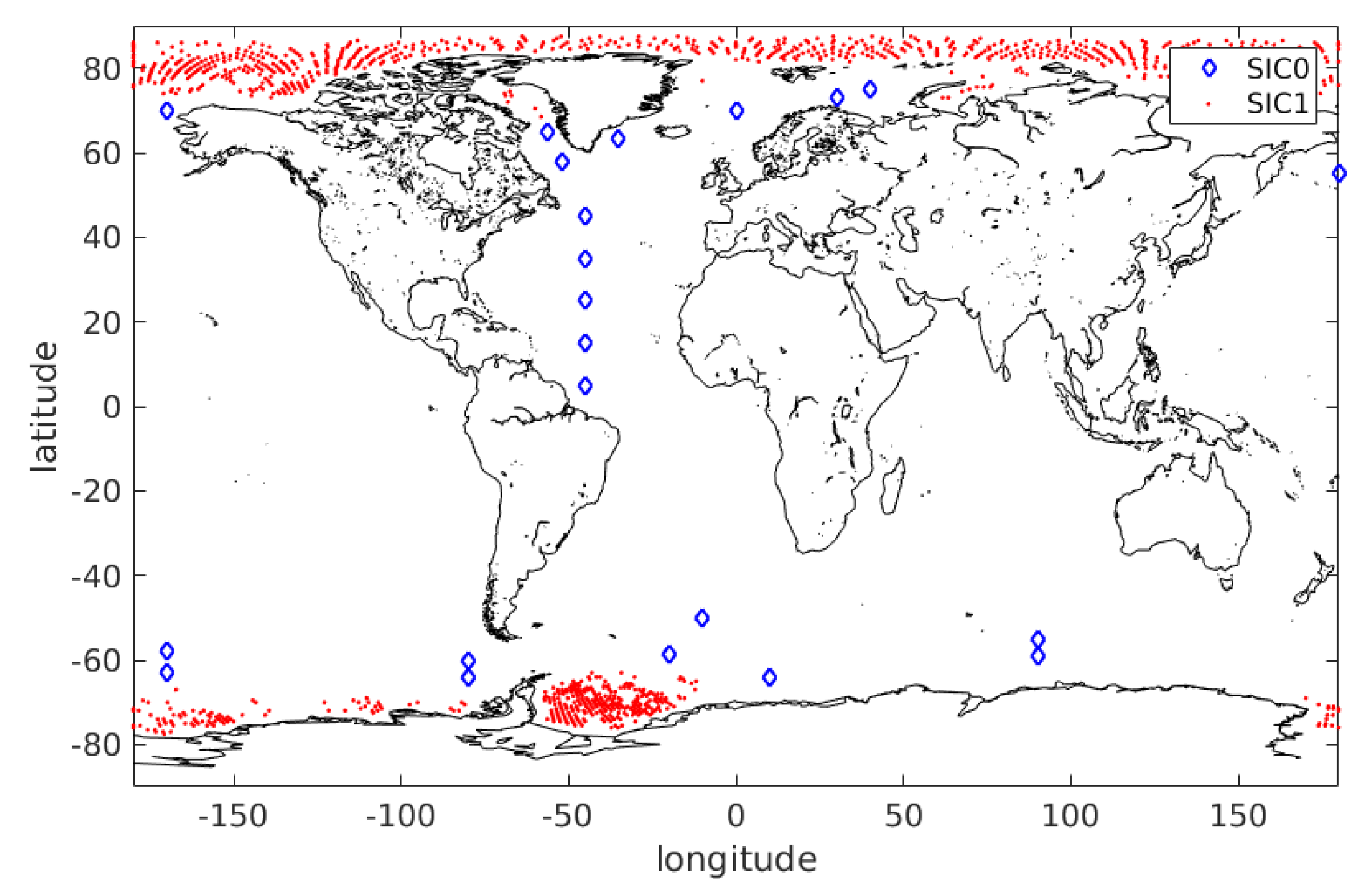
To identify areas of 100% ice (SIC1), the method used in the RRDP is based on ice drift dataset derived from radar observation (ENVISAT ASAR, Radarsat2 and Sentinel-1). Areas of ∼100×100 km² with convergence in the ice drift pattern on two consecutive days are selected. During winter, this will correspond to areas of total ice cover (assuming that it starts on day 1 with near 100% ice). In summer, the percentage of ice may be uncertain, as opening in the ice may appear. Areas with 0% ice are selected at ∼100 km away from the ice edge using ice-chart data. Then satellite microwave radiometer data with the footprint inside the selected areas of 0% and 100% are chosen for collocation.

The locations of the SIC0 and SIC1 observations are summarized in Figure 1. Note the presence of SIC0 data located at low latitudes which are not representative of polar ocean/sea ice margins and that are filtered out for our study. SIC0 dataset totalizes 26,289 collocations, and SIC1 dataset totalizes 2008 collocations.

The RRDP dataset gives direct access to the sensitivity of the observations to the characteristics of the sea ice. It has already been used in current SIC algorithms [15]. We use this database to compute the tie points used in our methodology, with their respective variances and covariances at different frequencies and polarizations, and to derive the linear forward model. Depending on the season, hemisphere, or ice types, some variability is expected in the microwave observations. Here, we will evaluate this variability to assess if the algorithm has to account for these environmental conditions or if a generic algorithm can be adopted.

The SIC0 and SIC1 data are available for two different radiometers AMSR-E and AMSR2, depending on the observation year. We prefer to use AMSR2 (operational since 2012) data as it is the current radiometer whereas AMSR-E (2002-2011) is not operational anymore.

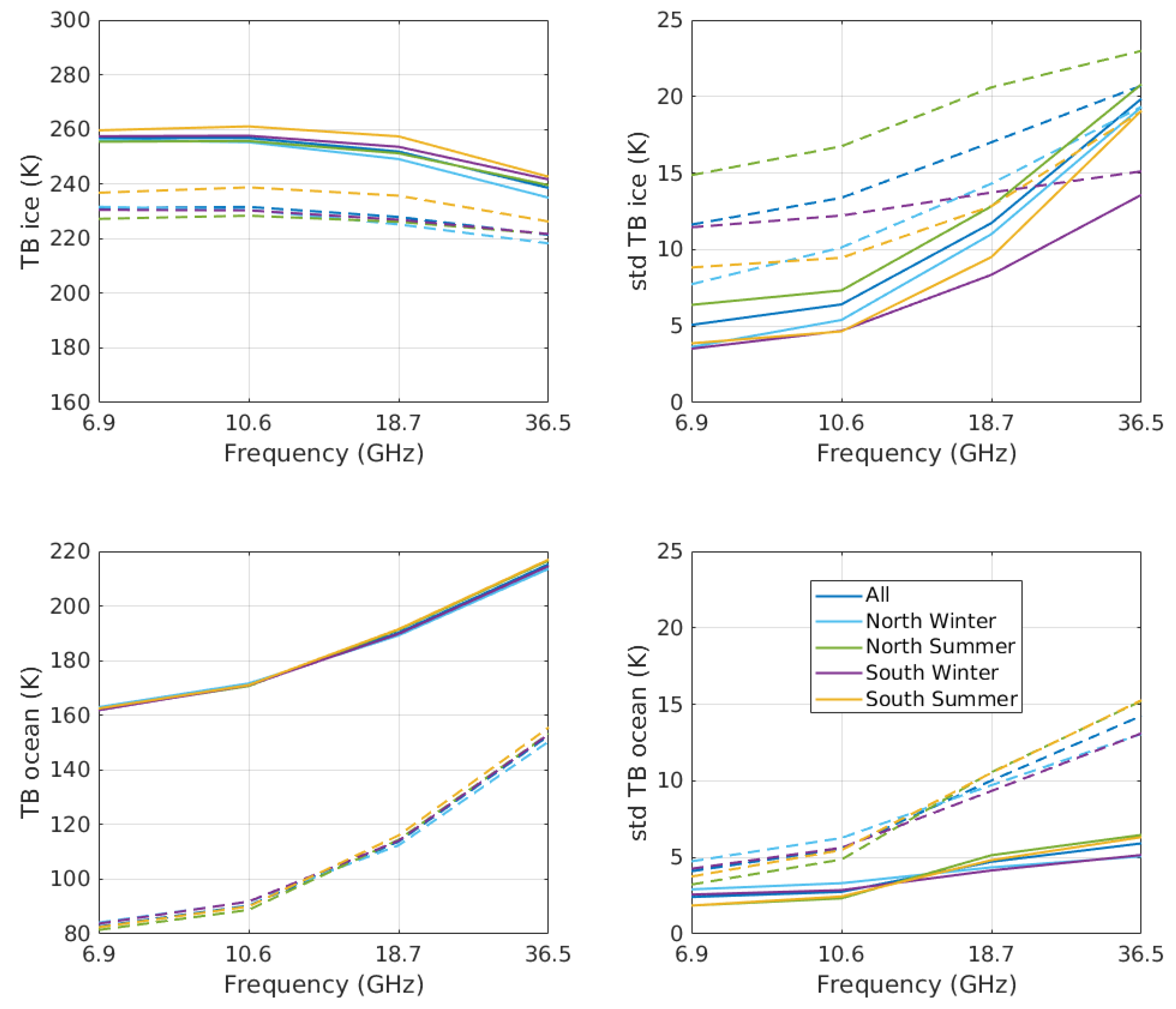
The mean ${\mathrm{TB}}_{ice}$ and ${\mathrm{TB}}_{ocean}$ (the respective tie points for SIC1 and SIC0) and their Standard Deviations (StD) are calculated from the RRDP. First, we compute the tie points using the complete dataset. Then, they are calculated restricting the data to a given season (winter or summer) and hemisphere (north or south). The results are shown in Figure 2. There are respectively 39%, 35%, 22%, and 4% of the SIC1 data in the boreal winter, in the boreal summer, in the austral winter, and in the austral summer. The differences between the tie points for the different seasons and hemispheres are small, and within the StDs. The StDs on the tie points are smaller for low frequencies, regardless of the season or hemisphere. The variability is smaller for winter than from summer: during winter, there is no melting processes and the sea ice emissivity is more stable. The variability of ${\mathrm{TB}}_{ice}$ is also smaller in the southern hemisphere where there is a few of Multi Year Ice (MYI) and almost only young and First Year Ice (FYI), contrarily to the northern hemisphere where both MYI and FYI are present at large extent. The tie points have also been computed for MYI and FYI separately (see Appendix A).

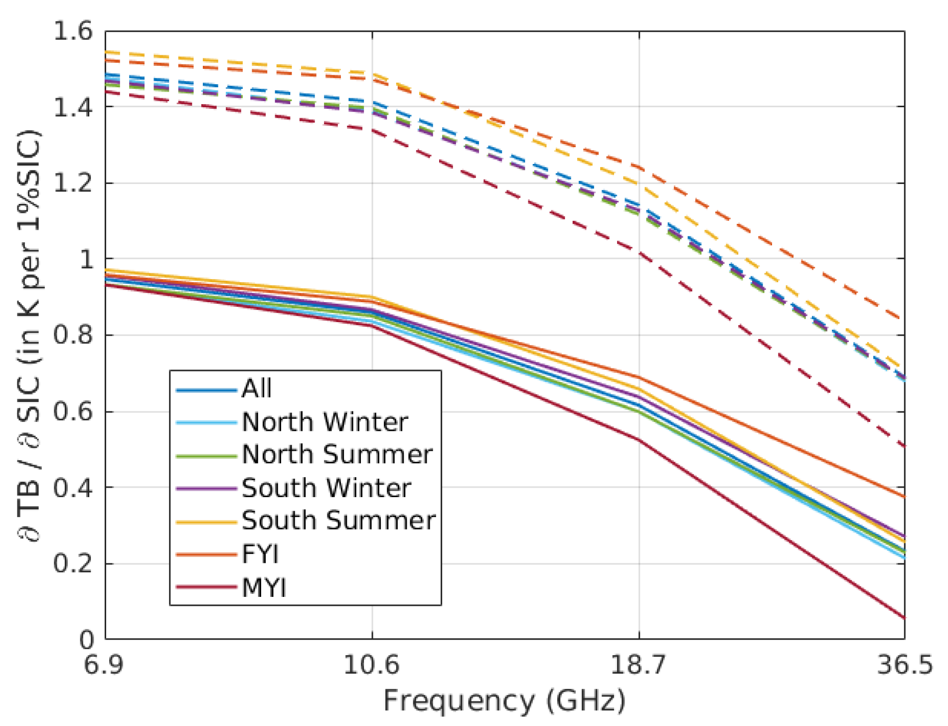
Figure 3 shows the Jacobians of SIC for different cases. The sensitivity to SIC is larger at low frequencies and at horizontal polarization. The ice type introduces the largest differences in the Jacobians for frequencies >10 GHz. This is partly related to the use of the 18 and 36 GHz channels to classify the ice types (see Appendix A).

The 6.9 and 10.6 GHz channels have the largest sensitivity to the SIC, regardless of the environmental conditions. That was expected given the larger differences between ${\mathrm{TB}}_{ocean}$ and ${\mathrm{TB}}_{ice}$ at these frequencies (see Figure 2). The 18 and 36 GHz channels are nevertheless often used today in SIC algorithms, because of their better spatial resolution even if they are less sensitive to SIC than the 6 and 10 GHz channels.

3. Results

In this section, we test the impact of different hypotheses on the retrieval, in terms of channel combination and tie point selection. At that point, we assume that all frequencies are observed with the same spatial resolution. The spatial resolution issue will be discussed in Section 4.

3.1. Sensitivity of the Sea Ice Concentration Retrieval to the Frequency Combinations

Different channel combinations can easily be tested within the optimal estimation method. The different combinations are evaluated by computing the SIC theoretical retrieval error StD (Equation (2)). Note that here, we assume that the spatial resolution is the same for all frequencies (the spatial resolution issue will be analyzed in Section 4). First, each frequency (both polarizations) is separately tested. Then, combinations are explored. The 6 + 10 GHz combination (both V and H polarizations) is evaluated: these two frequencies have a good sensitivity to the SIC and are not affected much by the atmosphere. The 18 + 36 GHz combination is extensively used by the current operational algorithms and is also tested. The combination of the four frequencies 6 + 10 + 18 + 36 GHz is also tested, for both polarizations for each frequencies. It is expected that adding channels to the algorithm increases the amount of information provided to the retrieval and therefore decreases the theoretical retrieval error. Note that in this subsection, all data from AMSR2 in the RRDP are used.

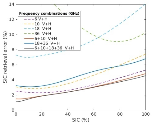
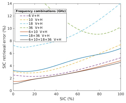
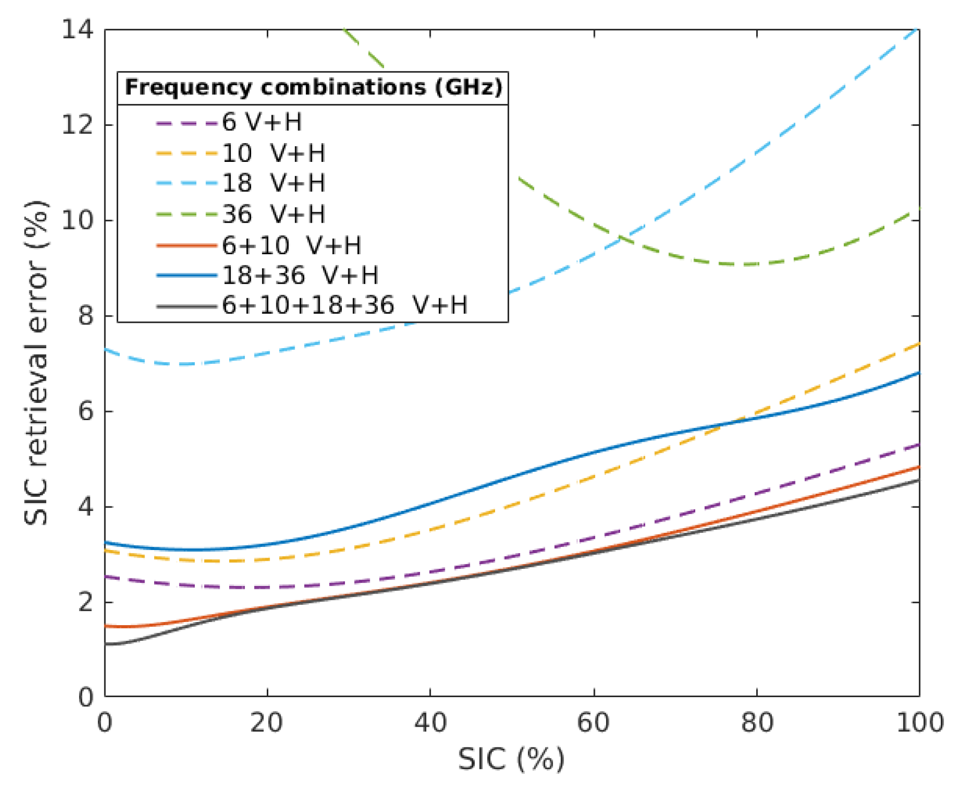
Figure 4 presents the SIC theoretical retrieval error StD as a function of SIC for the different channel combinations. For a single frequency algorithm, the 6 GHz provides the lowest error and this is in agreement with the results from Ivanova et al. [16]. With increasing frequency, the single frequency retrieval error increases, with significant errors at 18 and 36 GHz. By combining the 18 and the 36 GHz channels, the SIC theoretical retrieval error is between 3% and 6.8%, a significant improvement compared to the SIC retrieval error using either frequency alone. The combination of the 6 + 10 GHz channels gives a SIC theoretical retrieval error between 1.5 and 4.8%, which is better than the 18 + 36 GHz combination. The full combination of all the frequencies gives a SIC retrieval error between 1.1% and 4.5%, very close to the results obtained with the 6 + 10 GHz combination.

The combinations of 6 + 10 GHz and 18 + 36 GHz will be tested further in the following. First these combinations show good potential for the SIC retrieval in terms of errors. Second, the CIMR instrument will have the same spatial resolutions, for the 6 and the 10 GHz (15 km), and the 18 and 36 GHz (∼5 km) (see Table 1). A method will be suggested in Section 4 to merge the results of the 6 + 10 GHz algorithm at 15 km with the results of the 18 + 36 GHz algorithm at ∼5 km.

3.2. Impact of the Tie Points

There are recurrent discussions in the sea ice remote sensing community on the use of regionally or seasonally varying tie points in the retrievals. Operational methods tend to dynamically update the tie points in the algorithm to account for the changes in sea ice and ocean conditions, in space and time. Note that in the current algorithms, when the tie points are changed, it is not mentioned that the associated covariances are modified. In our methodology, the results of the retrievals depend on the tie point values as well as on their variability. The tie point selection will directly impact both the systematic (i.e., the bias) and random (i.e., the StD) errors of the retrieval.

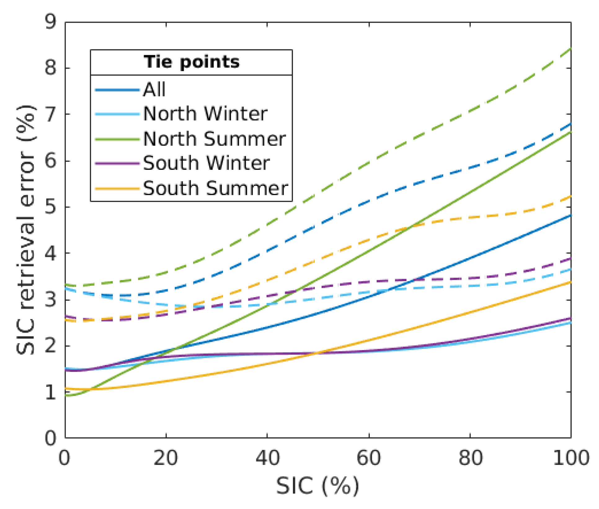
First, we estimate the impact of the tie point changes on the retrieval random errors. Figure 5 shows the SIC theoretical retrieval error as a function of SIC for the 6 + 10 GHz and the 18 + 36 GHz combinations and for different tie points that have been computed using different seasons (winter or summer) or hemispheres (north or south). The changes in the tie points and their covariances essentially affect the retrieval error for high SIC (with differences up to 4% for 100% SIC). The SIC theoretical retrieval errors are smaller using the winter season tie points, as the sea ice condition is more stable during winter. By the same token, during summer the SIC retrieval in the Southern hemisphere shows lower errors because of the lower variability of the sea ice in this hemisphere.

To quantify the impact of the tie points on the retrieval error (and to verify the theoretical retrieval error calculation), the retrieval algorithm of Equation (1) is applied to the TBs in the RRDP, for different tie point selections. At 100% SIC (resp., 0% SIC) in the RRDP (or a subset of it), the mean of the retrieved SIC should be 100% (resp., 0% SIC) with a StD equal to the theoretical retrieval error StD shown in Figure 5, when the tie points used in the forward model are representative of the whole database. This test is performed using different subsets of the RRDP data: (1) to calculate the tie points and their covariances, and (2) to apply the retrieval algorithm. 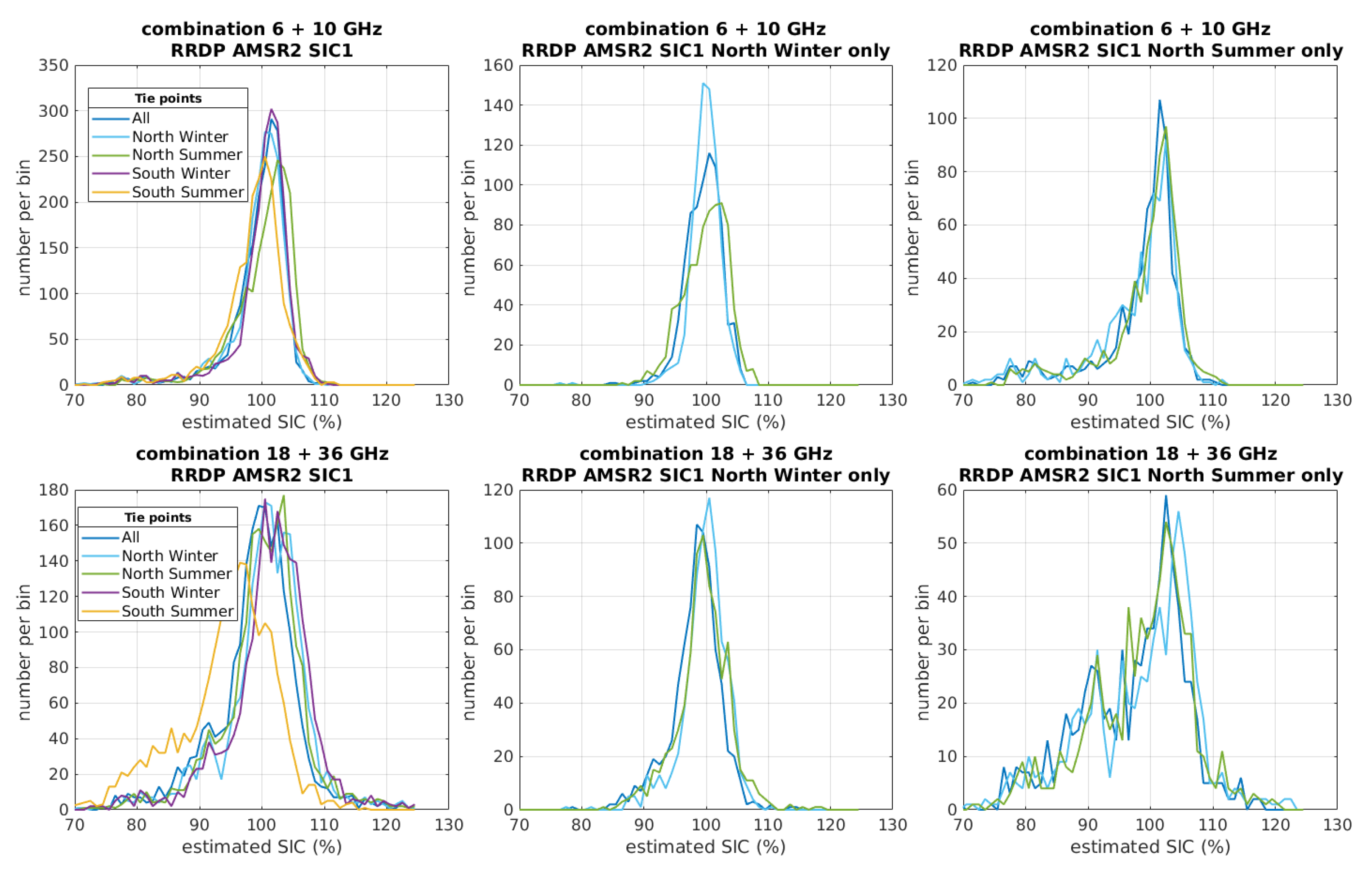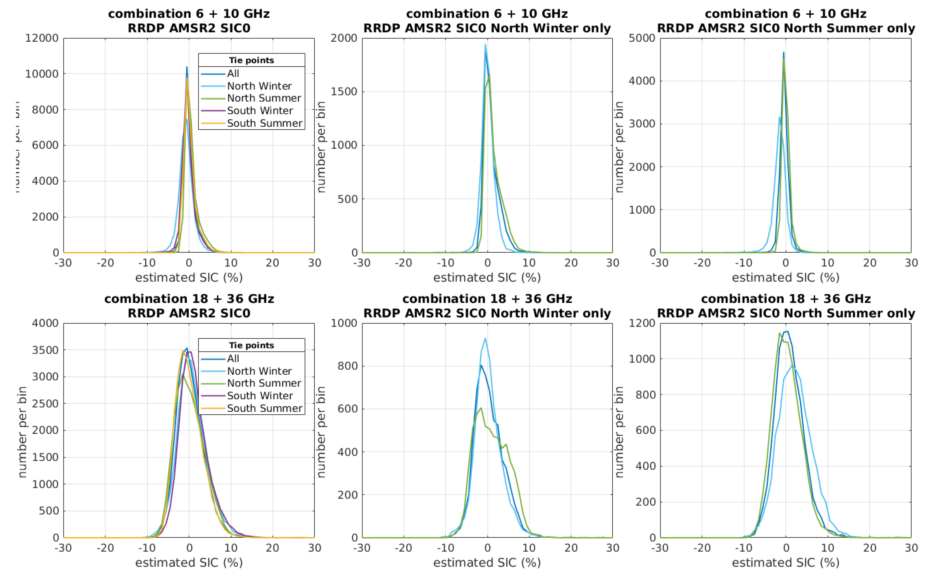Figure 6 and Figure 7 illustrate the distribution of the retrieved SIC with our algorithm using different tie points applied to different subset of the RRDP for 100% and 0% SIC. The Appendix B provides the corresponding statistics for 100% SIC. Note that here the SIC values can be lower than 0% or larger than 100%. This is because we choose to not constrain the inversion in order to properly evaluate the precision of the algorithm. When applied operationally, the algorithm has to be constrained to not provide these non-physical values.

First, it is clear that the 6+10GHz combination is not very sensitive to the tie point selection and to the season and location. The mean of the distribution is centered very close to 100% and the width of the histograms is rather narrow (see also the corresponding numbers in

Table A1. Results of the retrieval illustrated in Figure 6, in terms of Bias (%) and StD (%) for the combination of 6 and 10 GHz, and 18 and 36 GHz channels.

Combinations	Bias(%); StD(%) of the Retrieved SIC
and	Using AMSR2 SIC1 Data
Tie Points		North	North	South	South
	all	Winter	Summer	Winter	Summer
6 + 10 GHz
AMSR2	0; 4.8	0; 2.8	−2; 6.6	0; 2.8	1; 3.4
AMSR2 North Winter	−1; 5.2	0; 2.5	−2; 7.3	−1; 3.1	1; 4.2
AMSR2 North Summer	0; 4.9	0; 3.5	−1; 6.4	1; 3.3	3; 3.7
AMSR2 South Winter	0; 5.0	1; 2.8	−1; 7.1	0; 2.6	1; 3.8
AMSR2 South Summer	−1; 5.2	−1; 3.9	-2; 7.1	−1; 3.7	0; 3.3
18 + 36 GHz
AMSR2	−1; 6.8	−2; 4.0	−3; 8.5	−3; 4.4	4; 6.1
AMSR2 North Winter	1; 7.4	0; 3.7	−2; 9.1	−1; 3.9	6; 7.0
AMSR2 North Summer	0; 6.9	0; 4.3	−2; 8.2	−1; 4.6	5; 6.6
AMSR2 South Winter	1; 7.6	1; 3.8	−1; 9.3	0; 3.9	7; 7.3
AMSR2 South Summer	−6; 7.7	−7; 5.2	−8; 9.9	−7; 5.3	−1; 5.5

). This means that the low frequency algorithm is robust to changes in seasons, hemispheres and does not benefit much from a dynamic modification of the tie points. During summer, the results are marginally less good, but it is specified in the RRDP that the SIC at 100% is not guaranteed and during this season there are more complex processes in the sea ice impacting the TBs.

Second, as expected, the 18+36GHz combination algorithm is affected more by changes in the season and hemisphere, due to the larger variability of the radiometric signatures over sea ice and ocean at these frequencies. Changes in the tie points can induce biases in the SIC estimate up to ∼8%, with related StDs up to 9%.

Note that the StDs of the retrieved SIC (Table A1) are exactly the same than the theoretical retrieval error StDs predicted with the optimal estimation scheme (Figure 5), as expected.

The SIC retrieval using the 6 + 10 GHz combination has a lower bias and StD than using the 18 + 36 GHz combination. The algorithm with the 6 + 10 GHz combination is rather insensitive to changes in the tie points. A single and simple algorithm can be applied at these frequencies, regardless of the environment, with a low theoretical retrieval error. The algorithm using 18 + 36 GHz shows slightly larger retrieval errors with a bias that depends on the season and the hemisphere. Nevertheless the 18 + 36 GHz channels benefit from a better spatial resolution than 6 + 10 GHz channels. In the following section, we describe a new method to benefit from both the good sensitivity of the 6 + 10 GHz combination and the better spatial resolution of the 18 + 36 GHz combination.

4. Discussion

4.1. A Data Fusion Method to Solve the Spatial Resolution Issue

The spatial resolution of the SIC estimation is equal to the spatial resolution of the satellite observations used in the retrieval. In most algorithms, different frequencies are used that do not have the same spatial resolution. Therefore, an unique spatial resolution for the SIC results is not easily to obtain. For CIMR and AMSR2, there is a factor of 3 and 5 respectively in terms of spatial resolution between the 6 GHz and the 36 GHz channels. With the CIMR mission we will benefit from the same spatial resolution (15 km) for the 6 and 10 GHz channels, and the same spatial resolution (5 km) for the 18 and 36 GHz channels. As demonstrated in the previous section, the SIC estimate with the combination of the 6 + 10 GHz is more robust to the changes of season and hemisphere, less noisy and less biased than with the combination of 18 + 36 GHz. The objective is to benefit from both the high spatial resolution of the 18 + 36 GHz and the robustness of the 6 + 10 GHz, to estimate the SIC with maximum spatial resolution and a minimized error.

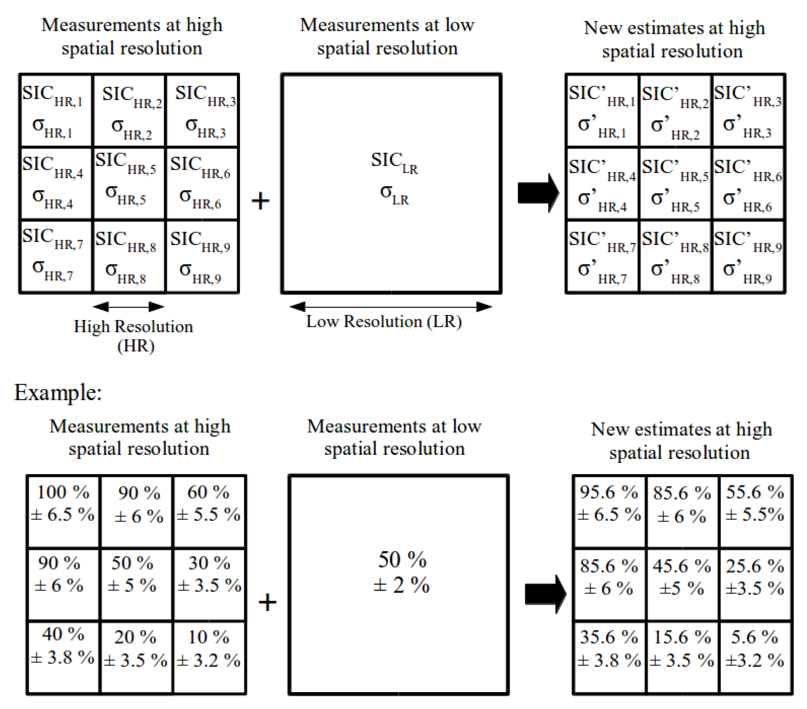
Here we propose a method to combine the SIC estimate at high resolution with the low resolution estimation. The SIC estimate at low resolution is used to correct the SIC estimates at high resolution that are within the low resolution pixel. We define:

• N = 9 the number of high resolution pixels contained in the low resolution pixel;
• $SI{C}_{HR}$ the SIC estimates at high resolution (5 km) and ${\sigma }_{HR}$ their corresponding retrieval error StDs;
• $SI{C}_{LR}$ the SIC estimate at low resolution (15 km), and ${\sigma }_{LR}$ its corresponding retrieval error StD.

In order to compare the low and the high resolution estimates, the high resolution is first upscaled by using a simple averaging:

$$SI{C}_{HR,mean}=\frac{1}{N}\sum _{i=1}^{N}SI{C}_{HR,i}$$

(6)

The uncertainty of this upscaled estimate is given by:

$${\sigma }_{HR,mean}=\sqrt{\sum _{i=1}^N{\sigma }_{HR,i}^2}$$

(7)

The reference for the SIC estimate at low resolution is then computed using a weighted average:

$$SI{C}_{LR,weighted}=\frac{{\sigma }_{LR}^2}{{\sigma }_{LR}^2+{\sigma }_{HR,mean}^2}SI{C}_{HR,mean}+\frac{{\sigma }_{HR,mean}^2}{{\sigma }_{LR}^2+{\sigma }_{HR,mean}^2}SI{C}_{LR}$$

(8)

based on the retrieval uncertainties (StDs) of the low and the upscaled resolution estimates. $SI{C}_{LR,weighted}$ is the a low resolution reference SIC based on the low and the high resolution. It is our best estimate of the SIC at the low resolution based on all the available satellite data.

Then, the $SI{C}_{HR}$ are bias-corrected towards this $SI{C}_{LR,weighted}$ value: For each high resolution pixel contained in the low resolution pixel, the new SIC estimates $SI{C}_{HR,fusion}$ are computed following:

$$SI{C}_{HR,fusion}=SI{C}_{HR}+(SI{C}_{LR,weighted}-SI{C}_{HR,mean})$$

(9)

This ensures that no bias exist between $SI{C}_{HR,fusion}$ and $SI{C}_{LR,weighted}$.

The new SIC estimations $SI{C}_{HR,fusion}$ are therefore more accurate, as they have been corrected to be closer to the low resolution SIC estimate, and the spatial pattern from the high resolution is preserved. This method does not impact the retrieval error StDs of the $SI{C}_{HR}$ estimations (only a bias correction was applied to them) therefore ${\sigma }_{HR,fusion}={\sigma }_{HR}$.

4.2. Example with a Theoretical Test Scene

A theoretical scene test is proposed using the CIMR mission configuration. The SIC estimates are given with their corresponding theoretical retrieval errors for the high resolution and the low resolution (we use the errors presented in Figure 5, with the tie points computed from all AMSR2 data). Within the CIMR configuration, the high resolution SIC estimations are retrieved from the 18 + 36 GHz combination at 5 km, and the low resolution SIC estimations from the 6 + 10 GHz combination at 15 km, therefore N = 9. For high resolution estimates, we use the theoretical retrieval error StDs (${\sigma }_{HR}$) of the 18 + 36 GHz combination. For the low resolution estimate, we use the theoretical retrieval error StD (${\sigma }_{LR}$) of the 6 + 10 GHz combination. Figure 8 presents the method, applied on a test scene, along with the corresponding results.

We observe that the SIC estimations at high resolution are corrected to be closer to the SIC estimation at low resolution when averaged. For the situation considered in Figure 8: $SI{C}_{LR}=50\%$, $SI{C}_{HR,mean}=54.4\%$, and we compute $SI{C}_{LR,weighted}=50.1\%$. Then, the correction applied on the $SI{C}_{HR}$ estimates is $-4.4\%$. All the high resolution pixels contained in the same low resolution pixel are corrected the same way. Note that the method takes into account the initial retrieval errors (${\sigma }_{LR}$ and ${\sigma }_{HR}$), therefore the correction depends on the situation. This method allows to keep the fine spatial structure given by the high resolution SIC estimates using the 18 + 36 GHz combination while reducing the bias using the 6 + 10 GHz results.

5. Conclusions

We propose a new SIC retrieval based on passive microwave observations called IceCREAM algorithm. This new methodology is particularly adapted for the CIMR mission. It follows the optimal estimation [17,18]. This allows using several channels and different channel combinations to retrieve the SIC. With the optimal estimation scheme, the SIC retrieval estimate is systematically given with its retrieval error StD. The method uses as forward model a linear combination of the ${\mathrm{TB}}_{ice}$ and ${\mathrm{TB}}_{ocean}$ which are called tie points and correspond to the mean TB of ice or ocean at a given frequency. These tie points and their variabilities have been estimated using the RRDP for different seasons (winter and summer), locations (Northern and Southern hemispheres). The tie points used for the SIC retrieval have a small impact (for most of the cases less than 1%) on the retrieved SIC error.

Then a data fusion method is developed to combine the accurate SIC estimate of the 6 + 10 GHz combination with the high resolution estimate of the 18 + 36 GHz. The SIC estimates at high resolution are debiased to be closer to the accurate SIC estimate at low resolution. The systematic errors are decreased, and the spatial pattern at high resolution is preserved. This new data fusion method is particularly well suited to the CIMR mission.