Joint Spatial-spectral Resolution Enhancement of Multispectral Images with Spectral Matrix Factorization and Spatial Sparsity Constraints

Abstract

This paper presents a joint spatial-spectral resolution enhancement technique to improve the resolution of multispectral images in the spatial and spectral domain simultaneously. Reconstructed hyperspectral images (HSIs) from an input multispectral image represent the same scene in higher spatial resolution, with more spectral bands of narrower wavelength width than the input multispectral image. Many existing improvement techniques focus on spatial- or spectral-resolution enhancement, which may cause spectral distortions and spatial inconsistency. The proposed scheme introduces virtual intermediate variables to formulate a spectral observation model and a spatial observation model. The models alternately solve spectral dictionary and abundances to reconstruct desired high-resolution HSIs. An initial spectral dictionary is trained from prior HSIs captured in different landscapes. A spatial dictionary trained from a panchromatic image and its sparse coefficients provide high spatial-resolution information. The sparse coefficients are used as constraints to obtain high spatial-resolution abundances. Experiments performed on simulated datasets from AVIRIS/Landsat 7 and a real Hyperion/ALI dataset demonstrate that the proposed method outperforms the state-of-the-art spatial- and spectral-resolution enhancement methods. The proposed method also worked well for combination of exiting spatial- and spectral-resolution enhancement methods.

1. Introduction

Hyperspectral imaging has demonstrated its usefulness in various earth observation applications, such as landscape classification [1], object detection [2], and environmental monitoring [3]. Hyperspectral sensors collect contiguous spectral bands over the visible to the infrared wavelength ranges. Rich spectral characteristics in hyperspectral image (HSI) are beneficial in identifying and classifying different materials and landscapes [4]. In hyperspectral imaging, there is a trade-off between spatial and spectral resolutions. The spatial resolution of spaceborne hyperspectral images (HSIs) is always lower than multispectral images (MSIs) and panchromatic (PAN) images. Instantaneous field of view (IFoV) should be enlarged to achieve acceptable signal-to-noise ratio (SNR) with narrow spectral bandwidth [5]. For example, the maximum spatial resolution of Sentinel 2 MSI is 10 m while the spatial resolution of Hyperion HSI is only 30 m. Low spatial resolution of HSI always results in mixed pixels and degrades the performance of subsequent applications, while spectral understanding and analysis are usually limited by low spectral resolution of MSIs or PAN images. Although earth observation remote sensing data have become increasingly available and the corresponding applications have attracted wide interests, there are existing challenges in acquiring images with simultaneously high spatial resolution and high spectral resolution [6]. Therefore, many research focuses on recovering high quality synthetic image from low resolution (LR) inputs, including spatial resolution improvement approaches [7,8,9,10,11,12,13,14,15,16,17,18,19] and spectral resolution enhancement techniques [20,21,22,23,24,25,26,27].

1.1. Spatial Resolution Improvement of HSI

Over past decades, several spatial improvement methods have been proposed based on the fusion of MSI and PAN images. Hyperspectral pan-sharpening improves spatial resolution of HSI by fusing LR HSI with a high resolution (HR) PAN image covering a spectral range from the visible to the near infrared ranges [7]. Except for the classical hyperspectral pan-sharpening approaches such as component substitution (CS) methods [8], multi-resolution analysis (MRA) methods [9], and model based optimization methods [10,11], deep learning, particularly convolutional neural network (CNN), has been widely exploited in pan-sharpening tasks. In [12], a residual CNN model is designed to describe the mapping between LR/HR MSI pairs and PAN image. Yuan et al. [13] proposed a multi-scale and multi-depth CNN (MSDCNN) for pan-sharpening, in which multi-scale feature extraction is used to reconstruct the HR MSI.

HSI fusion is another popular approach to spatial resolution improvement. A HR HSI is recovered by fusing a LR HSI with a HR MSI, where the HSI and MSI are assumed to be captured simultaneously for the same landscapes. Typical fusion methods based on the transform domain including the 2-D and 3-D wavelet transforms [14] can always result in heavy spectral distortions. Statistical methods are proposed by using a stochastic mixing model [15]. Another effective fusion method based on spectral unmixing recovers HR HSI using the endmembers/spectral dictionary from a LR HSI and the abundances from a HR MSI [16]. For example, Yokoya et al. [17] proposed a coupled non-negative matrix factorization (CNMF) method based on unsupervised spectral unmixing, where MS image and HSI are alternately unmixed using non-negative matrix factorization. In [18], a non-parametric Bayesian model is proposed using dictionary learning and sparse coding to achieve HR hyperspectral result. Dong et al. designed a non-negative structured sparse representation (NSSR) method [19]. The reconstructed HR HSI is formulated through estimating a non-negative spectral dictionary and its sparse coefficients. However, these fusion methods are limited to the same spatial coverage as the input image, therefore only HR HSI of the same spatial coverage as the input LR HSI can be obtained.

1.2. Spectral Resolution Enhancement Techniques

Despite various approaches to spatial resolution improvement techniques, only a few methods focus on spectral super-resolution. Spectral resolution enhancement reconstructs a HSI from a MSI or RGB image, where the recovered HSI and the input MSI/RGB image have the same spatial resolution and coverage [20]. Existing spectral resolution enhancement algorithms are categorized into hardware methods and reconstruction methods. The hardware methods achieve HSI from RGB/MSI through active light [21], tunable filters [22], and variable spectral responses provide by different RGB cameras [23]. Due to the requirement of modifying optics instruments or adding extra hardware equipment, such methods may not be suitable for remote sensing tasks. Several spectral reconstruction methods are proposed to improve spectral resolution. For example, a spectral resolution enhancement method (SREM) [24] recovers a HSI with wide swath by estimating spectral response matrix. Arad et al. [25] proposed a spectral resolution enhancement algorithm based on sparse representation, where a spectral dictionary is learned from prior HSIs through K-means singular value decomposition (K-SVD), and HSI is recovered from the input RGB image. The performance of this method is further boosted in [26] by exploiting with a shallow sparse representation framework. In [27], a convolutional neural network was introduced to learn an end-to-end spectral mapping between RGB image and HSI, which is proved to achieve better spectral resolution improvement results. Most spectral resolution improvement methods mentioned above only recover HSI from a RGB image, covering only the visible or part of the near-infrared spectral regions. Our previous work [20] proposed a spectral super-resolution approach over the full spectral range from 400 nm to 2500 nm. Spectral improvement strategy and spatial preservation strategy are introduced respectively to estimate spectral response relationship by prior MSI/HSI pairs, learn spectral dictionaries from HS priors and ensure consistency using spatial constraints.

Despite many applications requiring high-resolution HSIs with relatively short time intervals, existing spaceborne HSIs are only available in low spatial- and temporal-resolution as well as low revisit frequency. PAN images have high spatial resolution and MSIs come in high temporal resolution and revisit frequency [20]. Therefore, we can easily acquire high spatial resolution PAN images or high temporal resolution MSIs at different time or over different landscapes, which is challenging for spaceborne HS sensors. Most scenes captured using multispectral or panchromatic sensors do not have their corresponding HSIs. This paper proposes a joint spatial-spectral resolution enhancement method using PAN images and prior HSIs. The reconstructed HSI has the same spatial resolution as PAN image and the same spectral resolution as the prior HSIs. The proposed method not only improves the spatial- and spectral-resolution of the input image, but also creates a new HSI at different time or over different scenes, which provides new opportunities for earth observation.

Existing techniques aim at improving either spatial resolution or spectral resolution, not HR HSI by improving spatial- and spectral-resolution simultaneously. If resolution enhancement is performed step-by-step in the spatial- or the spectral domain, any defects and distortions transferred from the previous step will pose difficulties in eliminating the artifacts in the current step. So, the performance of their subsequent processing tasks will be degraded. Additionally, it will be challenging to unify spatial and spectral enhancement techniques into one framework to improve spatial- and spectral-resolution simultaneously. A low spatial resolution MSI with a few spectral bands are required to recover a HSI of high spatial resolution and of more than 200 bands, which is obviously a highly ill-posed converse problem. The proposed method reduces artifacts and distortions using spatial features from PAN image and spectral signatures from prior HSIs. Combined spectral unmixing for unified spatial and spectral improvements ensures accurate spectral characteristics for subsequent applications.

The proposed scheme recovers a high spatial resolution HSI from an input low spatial resolution MSI based on high spatial-spectral correlation in an input low resolution MSI and the desired high quality HSI. Each pixel in the desired HSI can be represented by a linear combination of a few pure spectral signatures extracted from a spectral dictionary [28]. The pixels in the input LR MSI are assumed to be highly correlated with the HR ones in the desired high quality HSI [29]. Figure 1 shows a joint spatial-spectral resolution enhancement algorithm proposed in this paper to simultaneously improve spatial- and spectral resolution. Spectral and spatial improvement are combined into a unified framework based on formulating spectral observation model and spatial observation model. In this work, an input LR MSI and the desired HR HSI are denoted as LSpaLSpe and HSpaHSpe, respectively. Two virtual intermediate variables are designed for a more comprehensive description of the spatial and the spectral observation models. These two virtual intermediate variables are denoted as HSpaLSpe and LSpaHSpe, respectively. HSpaLSpe represents high spatial resolution but low spectral resolution MSI, and LSpaHSpe indicates low spatial resolution but high spectral resolution HSI. HSpaLSpe has the same spatial resolution as the desired HR HSI, considered as the spatial improvement result of the input LR MSI. While LSpaHSpe has the same spectral resolution as the desired HSI, considered as the spectral enhancement result of the input MSI. Desired HSI is decomposed by a linear combination of spectral signatures from spectral dictionary, where abundances describe the fractions of each spectral signature [28]. We assume that high spectral resolution dictionary is extracted from the LSpaHSpe HSI while the high spatial resolution abundances are extracted from HSpaLSpe MSI. So the spectral observation model, which describes spectral relationship scheme between the input MSI and the desired HSI, can be formulated via the virtual intermediate variable LSpaHSpe. The spatial observation model to describe the relationship between input MSI and desired HSI is built using HSpaLSpe. LSpaHSpe and HSpaLSpe are just virtual intermediate variables in this work, not necessary to be solved.

In the spectral observation model, spectral characteristics in the desired HSI can be extracted from LSpaHSpe. An initial spectral dictionary is acquired by adapting prior HSIs, captured using the same sensor as the desired HSI and cover different landscapes from the input image. The spectral dictionary is acquired from LSpaHSpe HSI. In the spatial observation model, a spatial dictionary is learned from a HR PAN image having the same spatial resolution as the desired HSI. The trained spatial dictionary is shared by the desired HSI and the HSpaLSpe MSI, while the relationship between their sparse coefficients is then exploited as spatial constraint to obtain high spatial resolution abundances. The sparse coefficients and abundances are solved using the feedback scheme in [11] to achieve more accurate results. In this paper, spectral- and spatial observation model are unified into a joint framework to alternately solve spectral dictionary and abundances. Spectral dictionary is updated using abundances while abundances are solved by the spectral dictionary in the previous iteration. These two steps can be used as constraints for each other to finally achieve joint spatial-spectral enhancement without solving for the virtual intermediate variables.

The contributions of the proposed algorithm are summarized as follows:

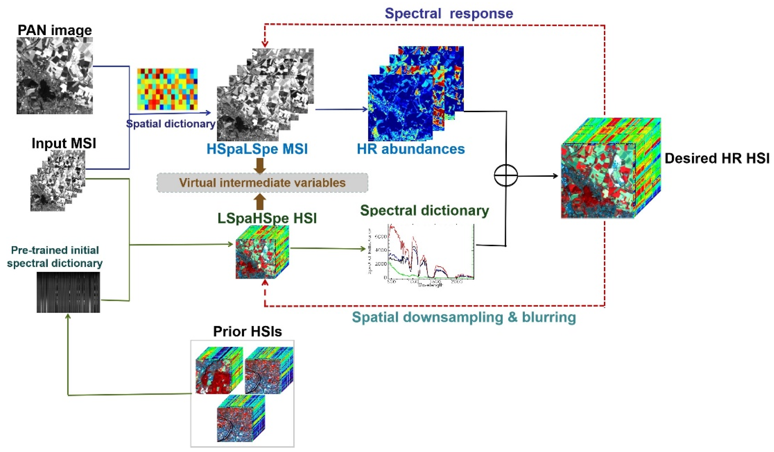
• Improves spatial and spectral resolution simultaneously, which unifies the spatial- and spectral enhancement steps in one framework taking high resolution spectral features and spatial information as the constraints for each other in an alternate solving process. To our best knowledge, this is the first attempt.
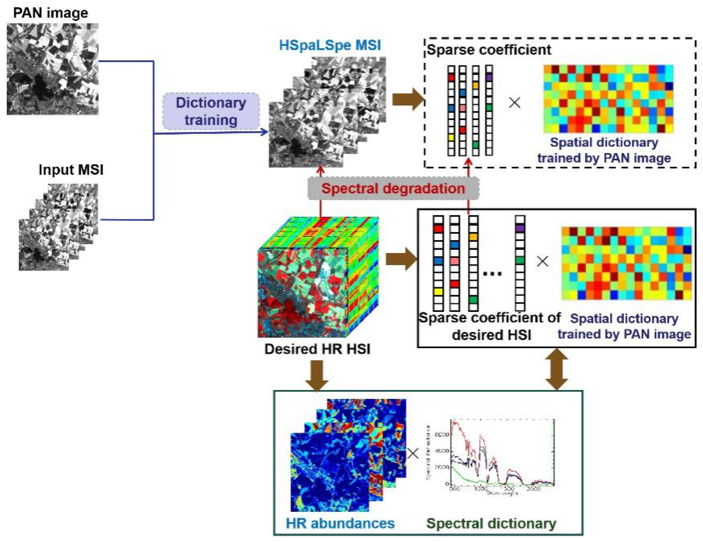
• Designed spectral and spatial observation models for the joint spatial and spectral enhancement problem. Virtual intermediate variables LSpaHSpe and HSpaLSpe are introduced in spectral and spatial observation models to find spectral/spatial relationships between input LR MSI and the desired HR HSI. The high spectral resolution dictionary and the corresponding high spatial resolution abundances are alternately solved to recover a high spatial and spectral resolution HSIs. LSpaHSpe and HSpaLSpe are only virtual intermediate variables without having to solve them in the proposed method.
• The proposed joint spatial-spectral enhancement algorithm is applied to real remote sensing data, such as ALI/Hyperion (30 m, 9 bands/ 30 m, 242 bands), for a target scene, the PAN image of ALI (10 m) is used to provide high spatial resolution features, while prior Hyperion HSIs (30 m, 242 bands) over different scenes are used to train spectral dictionary with high spectral resolution characteristics. So high spatial- and spectral resolution Hyperion data (10 m, 242 bands) of the target scene is achieved from the input LR ALI data (30 m, 9 bands).

The remainder of the paper is organized as follows. In Section 2, spatial observation and spectral observation models are introduced, respectively. The proposed joint spatial-spectral resolution enhancement method is presented in Section 3. In Section 4, we give the experimental results on both simulated and real datasets. Analyses and discussion are shown in Section 4 and finally conclusions are drawn in Section 5.

2. Spatial Observation Model and Spectral Observation Model

This section introduces spatial- and spectral observation models and two virtual intermediate variables LSpaHSpe HSI and HSpaLSpe MSI to alternately solve high resolution spectral dictionary and high spatial resolution abundances to recover desired HR HSIs.

2.1. Spatial Observation Model

In this paper, the virtual variable HSpaLSpe is assumed to have the same spatial resolution as the desired HSI and the same spectral resolution as the input MSI. HSpaLSpe is just an intermediate variable and is not necessary to be solved. PAN image contains abundant high-resolution spatial details and structures [30], used to train an over-completed spatial dictionary via sparse representation framework [31]. In Figure 2, virtual variable HSpaLSpe has the same spatial resolution as the desired HSI. HSpaLSpe and the desired HSI are assumed to share the same spatial dictionary. A spectral degradation mapping between HSpaLSpe and the desired HSI exists. The relationship between sparse coefficients of HSpaLSpe and the desired HSI obeys the spectral degradation mapping [5]. An interactive feedback framework [11] is also utilized in the spatial observation model to simultaneously deal with spatial processing and spectral unmixing.

2.2. Spectral Observation Model

Desired HSI consists of a few spectral signatures in a spectral dictionary [32]. In Figure 3, the virtual variable LSpaHSpe has the same spectral resolution as the desired HSI and the same spatial resolution as the input MSI. Like HSpaLSpe, LSpaHSpe is also considered as an intermediate variable and therefore not be solved in the proposed process. When the high spectral resolution image covering the same scene as the input image is not available, prior HSIs with different landscapes are used to estimate an initial spectral dictionary. The utilized prior HSIs have the same spatial resolution as LSpaHSpe and they are captured by the same sensor as the desired HSI. Due to the same spectral resolution, LSpaHSpe and the desired HSI share the same high-resolution spectral dictionary, and there is a spatial mapping scheme between them. Figure 3 shows that the mapping scheme of their abundances should be in accordance with the mapping scheme between two images.

3. Proposed Joint Spatial-spectral Enhancement Algorithm

The proposed joint spatial-spectral enhancement method combines spatial and spectral observation models into a unified framework to alternately solve spectral dictionary and abundances, from which the high spatial resolution and high spectral resolution image is achieved. HSIs and MSIs are denoted as 2-D matrices where each column represents an image of one spectral band. Input low spatial and spectral resolution MSI is denoted as $Y\in R^{m\times l}$, while $Z\in R^{M\times L}$ denotes the desired HSI. $\tilde{X}\in R^{m\times L}$ and $X\in R^{M\times l}$ denote LSpaHSpe and HSpaLSpe, respectively. $M$ and $m$ are respectively the number of pixels of high and low spatial images. $L$ and $l$ represent the number of spectral bands with $l<L$. The LSpaHSpe HSI is denoted as $\tilde{X}$, treated as the spatially degraded version of the desired HR HSI $Z$. Input MSI $Y$ is treated as spectrally degraded version of LSpaHSpe. $\tilde{X}$ and $Y$ can be formulated as:

$$\tilde{X}=TZ+{\mathsf{\mu }}_1,$$

(1)

$$Y=\tilde{X}M+{\mathsf{\mu }}_2$$

(2)

where $T\in R^{m\times M}$ denotes the spatial degradation matrix, which includes blurring and spatial down-sampling factor between the desired HSI $Z$ and LSpaHSpe HSI $\tilde{X}$. $M\in R^{L\times l}$ is the spectral response transform matrix between input MSI $Y$ and LSpaHSpe HSI $\tilde{X}$. In general, $T$ and $M$ are used as prior knowledge according to the sensors parameters. For real data, $T$ can be estimated using Gaussian point spread function and $M$ can be acquired using cross calibration [33]. ${\mathsf{\mu }}_1$ and ${\mathsf{\mu }}_2$ represent modeling errors and the noise. Another virtual intermediate variable HSpaLSpe image $X$ and input MSI $Y$ can be considered as spectrally degraded version of the desired HSI $Z$ and spatially degraded version of HSpaLSpe, respectively:

$$X=ZM+{\mathsf{\nu }}_1$$

(3)

$$Y=TX+{\mathsf{\nu }}_2$$

(4)

where ${\mathsf{\nu }}_1$ and ${\mathsf{\nu }}_2$ are modeling errors.

3.1. Formulation of Spectral Observation Model to Solve Spectral Dictionary

The spectral observation model is to obtain high spectral resolution dictionary. The spectrum of each pixel in the desired HSI $Z$ can be represented by a linear combination of spectral signatures, which is formulated as [32]:

$$z_i=a_i{D}_{spe}+n_i,$$

(5)

where $z_i$ is the spectrum of pixel $i$ in $Z$. $D_{spe}\in R^{K\times L}$ is the spectral dictionary containing K pure spectral signatures, $a_i$ represents fraction abundance which is assumed sparse, $n_i$ is modeling error. Since all images are used in 2-D forms [34], Equation (5) can be rewritten as a compact matrix form:

$$Z=A{D}_{spe}+n,$$

(6)

where $A$ denotes high spatial resolution fraction abundances, and $n$ is modeling error.

Due to the fact that $Z$ has the same spectral resolution as the LSpaHSpe image $\tilde{X}$, their underlying spectral signatures should be the same. Substituting (6) to (1), the spectral observation model can be expressed by

$$\tilde{X}\approx TA{D}_{spe}=\tilde{A}{D}_{spe},$$

(7)

As a result, spectral dictionary training can be solved by the following sparse non-negative matrix decomposition problem [19]:

$$\begin{array}{l}\{D_{spe},\tilde{A}\}=\arg \min \{\frac{1}{2}||\tilde{X}-\tilde{A}{D}_{spe}|{|}_F^2+\lambda ||\tilde{A}|{|}_1\}\\ s.t. {\tilde{a}}_i\ge 0,d_k^{}\ge 0\end{array},$$

(8)

where $\tilde{A}={[{\tilde{a}}_1,{\tilde{a}}_2,\dots ,{\tilde{a}}_M]}^T$ is the coefficient matrix described abundance of $\tilde{X}$, which is sparse in $l_1$ norm. Frobenius norm $||•{||}_F$ describes data fidelity and $\lambda$ is a positive parameter balancing the trade-off between sparseness and data fidelity terms. Both ${\tilde{a}}_i$ and the atoms in dictionary $D_{spe}$ are regularized to be non-negative, and the non-negative dictionary learning algorithm mentioned in [19] is employed to achieve the high resolution spectral dictionary $D_{spe}$ of the desired image $Z$.

3.2. Formulation of Spatial Observation Model to Solve abundances

Spatial observation model aims at estimating high spatial resolution abundances. The virtual intermediate variable HSpaLSpe image $X$ is used in this step. Assume that $z=\{z^1,z^2,\dots ,z^L\}$ is a 2-D patch matrix of $Z$, where $z^j(1\le j\le L)$ represent the HS patch of each band. $z^j$ can be represented as a linear combination of atoms via an over-completed spatial dictionary, which is expressed as follows based on sparse representation [35]:

$$z^j=\arg \min \{||z^j-D_{spa}{\alpha }^j|{|}_F^2+{\lambda }_1||{\alpha }^j|{|}_1\},$$

(9)

where $D_{spa}$ is the spatial dictionary trained by high spatial resolution PAN image using K-means SVD (K-SVD) algorithm [36]. ${\alpha }^j$ is a sparse coefficient vector. When the sparse formulation of one patch can be generalized to the patch matrix,

$$z=\arg \min \{||z-D_{spa}{\mathsf{\alpha }}_z|{|}_F^2+{\lambda }_1||{\mathsf{\alpha }}_z|{|}_1\},$$

(10)

where ${\mathsf{\alpha }}_z=\{{\alpha }^1,{\alpha }^2,\dots ,{\alpha }^L\}$ is the sparse coefficient matrix. ${\lambda }_1$ is the parameter of the sparse term.

The HSpaLSpe image $X$ has the same spatial resolution as $Z$, so the patch matrix $x=\{x^1,x^2,\dots ,x^l\}$ can be represented:

$$x=\arg \min \{||x-D_{spa}{\mathsf{\alpha }}_x|{|}_F^2+{\lambda }_2||{\mathsf{\alpha }}_x|{|}_1\},$$

(11)

where ${\mathsf{\alpha }}_x=\{{\alpha }^1,{\alpha }^2,\dots ,{\alpha }^l\}$ is the sparse coefficient matrix of $x$. ${\lambda }_2$ has the same function as ${\lambda }_1$. Substituting (3) into (10) and (11), the relationship between ${\mathsf{\alpha }}_z$ and ${\mathsf{\alpha }}_x$ can be obtained:

$${\mathsf{\alpha }}_x\approx {\mathsf{\alpha }}_{z}M,$$

(12)

Input image $Y$ is the spatial degradation version of $X$, the patch matrix $y=\{y^1,y^2,\dots ,y^l\}$, which covers the same scene as the patch matrix $x$, formulated in (13) by involving the spatial degradation relationship presented in (4):

$$y=\arg \min \{||y-T{D}_{spa}{\mathsf{\alpha }}_x|{|}_F^2+{\lambda }_2||{\mathsf{\alpha }}_x|{|}_1\},$$

(13)

Although HSpaLSpe image $X$ is not available in this work, the corresponding sparse coefficient matrix ${\mathsf{\alpha }}_x$ can be acquired by the input image $Y$ using the spatial degradation scheme between $Y$ and $X$. The sparse coefficient matrix ${\mathsf{\alpha }}_z$ can be obtained by (12). In Section 3.1, the desired image $Z$ can also be represented in spectral domain by a few spectral signatures weighted by corresponding fraction abundances. Spatial expression of $Z$ should be approximated to its spectral expression [11]:

$$R^{-1}{D}_{spa}{\mathsf{\alpha }}_z\approx A{D}_{spe},$$

(14)

where $R$ represents the extraction operator used to extract overlapping patch matrix from $Z$. The sparse coefficient matrix is used as spatial constraint to achieve high spatial resolution abundance $A$ of the desired HSI $Z$, where ${\mathsf{\alpha }}_x$ and $A$ are iteratively solved to obtain more accurate results with less distortions.

3.3. Joint Spatial-spectral Enhancement Algorithm

The proposed method recovers high resolution HSI $Z$ from the low spatial resolution and low spectral resolution input MSI $Y$, through which the spatial and spectral resolution are jointly improved. LSpaHSpe image $\tilde{X}$ and HSpaLSpe image $X$ are introduced as virtual variables which describes low spatial resolution but high spectral resolution image (HSI) and high spatial resolution but low spectral resolution image (MSI), respectively. $\tilde{X}$ is used to build the spectral observation model and $X$ is exploited to describe the spatial observation model, from which high resolution spectral dictionary $D_{spe}$ and high spatial resolution abundance $A$ are estimated alternately to achieve the desired HSI $Z$ with both high spatial and spectral resolution and less distortions.

As described in Section 3.1, the high spectral resolution dictionary $D_{spe}$ can be solved using $\tilde{X}$ via the non-negative dictionary learning algorithm, where $\tilde{X}$ is assumed to cover the same landscapes as the input MSI and the desired HSI. However, $\tilde{X}$ is a virtual variable that is unavailable in real cases. To obtain the high spectral resolution dictionary, prior HSIs, covering different landscapes, are used to train an initial spectral dictionary $D_{spe,0}$ in the first iteration. These prior HSIs are assumed to have the same spatial resolution as the input MSI and the same spectral resolution as the desired HSI. So, the initial spectral dictionary can be trained:

$$\begin{array}{l}\{D_{spe,0},B\}=\arg \min \{\frac{1}{2}||H-B{D}_{spe,0}|{|}_F^2+\lambda ||B|{|}_1\}\\ s.t. b_i\ge 0,d_k^{}\ge 0\end{array}$$

(15)

where $H$ represents the prior HSI, $B={[b_1,b_2,\dots ,b_M]}^T$ is the sparse abundance, and $\lambda$ is a positive parameter.

In Section 3.2, HSpaLSpe image $X$ is used to establish the spatial observation model to estimate high spatial resolution abundance $A$, where spatial sparse information of $Z$ is used as constraints to achieve more accurate result with less distortions. The sparse coefficient matrix ${\mathsf{\alpha }}_z$ of $Z$ is obtained by combing (12) and (13).

$$\{{\mathsf{\alpha }}_x,{\mathsf{\alpha }}_z\}=\arg \min \{||y-T{D}_{spa}{\mathsf{\alpha }}_x|{|}_F^2+{\lambda }_2||{\mathsf{\alpha }}_x|{|}_1+\beta ||{\mathsf{\alpha }}_x-{\mathsf{\alpha }}_{z}M|{|}_F^2\},$$

(16)

where y is the patch matrix in the input MSI $Y$,$D_{spa}$ is spatial dictionary trained by high spatial resolution PAN image ($Z$ should have the same spatial resolution as the PAN image). ${\mathsf{\alpha }}_x$ and ${\mathsf{\alpha }}_z$ are sparse coefficient matrices of the $X$ and $Z$, respectively. Parameter ${\lambda }_2$ balances sparsity and representation error and $\beta$ controls the spectral degradation of ${\mathsf{\alpha }}_x$ and ${\mathsf{\alpha }}_z$. The patch matrix $y$ is directly extracted from $Y$, and it is assumed to be accurate. So it helps to achieve more accurate spatial sparse information of the desired image.

The spectral expression and spatial representation of $Z$ should be approximated. The solved sparse coefficient matrix ${\mathsf{\alpha }}_z$ is exploited as spatial constraint to obtain high resolution abundance $A$ and simultaneously improve the accuracy of ${\mathsf{\alpha }}_z$ and $A$, the idea of which has already been proposed in our previous work [11]. The objective function of $A$ is written by using (14):

$$\{{\mathsf{\alpha }}_z,A\}=\arg \min \{||A{D}_{spe}-R^{-1}{D}_{spa}{\mathsf{\alpha }}_z|{|}_F^2+\eta ||A|{|}_1+\epsilon ||{\mathsf{\alpha }}_z|{|}_1\},$$

(17)

where $R^{-1}$ represents the patch matrix extraction factor. $\eta$ is the weight of abundance sparsity and $\epsilon$ is the parameter of spatial sparsity.

In this paper, spectral dictionary $D_{spe}$ and abundance $A$ are alternately solved. Using (14)-(15), the objective function of $D_{spe}$ is defined as (except the first iteration):

$$\{D_{spe},A\}=\arg \min \{||A{D}_{spe}-R^{-1}{D}_{spa}{\mathsf{\alpha }}_z|{|}_F^2+\mu ||A|{|}_1\},$$

(18)

where $\mu$ is the weight of abundance sparsity.

3.4. Solver

There are four objective functions that need to be solved, including the solution of initial spectral dictionary $D_{spe,0}$ in (15), the solution of spatial sparse information ${\mathsf{\alpha }}_z$ in (16), the solution of high spatial resolution abundance $A$ in (17) and the solution of high resolution spectral dictionary $D_{spe}$ in (18). These multiple variable objective functions are convex and unique solutions can be solved by variable splitting and alternate optimization [37].

3.4.1. Solution of Initial Spectral Dictionary $D_{spe,0}$

The objective function of initial spectral dictionary $D_{spe,0}$ in (15) can be solved using the non-negative dictionary learning algorithm proposed in [19], where each dictionary atom is updated via a closed-form solution. So, the optimization problem in (15) is divided into two sub-problems:

(1)

Solve $B$ with respect to a fixed $D_{spe,0}$

$$B=\arg \min \{\frac{1}{2}||H-B{D}_{spe,0}|{|}_F^2+\lambda ||B|{|}_1\}s.t. b_i\ge 0,$$

(19)

Equation (19) is solved by ADMM [38] for a fast convergence rate [39].

(2)

Update $D_{spe,0}$ with respect to a fixed $B$

$$D_{spe,0}=\arg \min \frac{1}{2}||H-B{D}_{spe,0}|{|}_F^{2}s.t. d_k\ge 0,$$

(20)

Equation (20) is solved via block coordinate descent which updates one atom in each iteration using the non-negative constraint [40].

3.4.2. Solution of Spatial Sparse Information ${\mathsf{\alpha }}_z$

The objective function of spatial sparse information ${\mathsf{\alpha }}_z$ in (16) can be divided into following two sub-problems:

(1)

Solve spatial sparse coefficient matrix ${\mathsf{\alpha }}_x$

$${\mathsf{\alpha }}_x=\arg \min \{||y-T{D}_{spa}{\mathsf{\alpha }}_x|{|}_F^2+{\lambda }_2||{\mathsf{\alpha }}_x|{|}_1\},$$

(21)

It is a sparse coding problem that can be solved by alternately learning $D_{spa}$ from the high spatial resolution PAN image using K-SVD [36] and estimating ${\mathsf{\alpha }}_x$ using OMP [41].

(2)

Solve spatial sparse coefficient matrix ${\mathsf{\alpha }}_z$ with respect to a fixed ${\mathsf{\alpha }}_x$

$${\mathsf{\alpha }}_z=\arg \min ||{\mathsf{\alpha }}_x-{\mathsf{\alpha }}_{z}M|{|}_F^2,$$

(22)

The optimization function in (22) can be directly solved via least square method [42].

3.4.3. Solution of High Spatial Resolution Abundance $A$

The objective function of high spatial resolution abundance $A$ in (17) is divided into following two sub-problems.

(1)

Solve $A$ with respect to a fixed ${\mathsf{\alpha }}_z$

$$A=\arg \min \{||A{D}_{spe}-R^{-1}{D}_{spa}{\mathsf{\alpha }}_z|{|}_F^2+\eta ||A|{|}_1\},$$

(23)

(2)

Solve ${\mathsf{\alpha }}_z$ with respect to a fixed $A$

$${\mathsf{\alpha }}_z=\arg \min \{||A{D}_{spe}-R^{-1}{D}_{spa}{\mathsf{\alpha }}_z|{|}_F^2+\epsilon ||{\mathsf{\alpha }}_z|{|}_1\},$$

(24)

Both of them are sparse coding optimization problems. Equation (23) is solved via ADMM and Equation (24) is solved by OMP.

3.4.4. Solution of High Resolution Spectral Dictionary $D_{spe}$

The objective function of high resolution spectral dictionary $D_{spe}$ in (18) is divided into following two sub-problems.

(1)

Update $D_{spe}$ with respect to a fixed $A$

$$D_{spe}=\arg \min ||A{D}_{spe}-R^{-1}{D}_{spa}{\mathsf{\alpha }}_z|{|}_F^2,$$

(25)

Equation (25) can be solved by block coordinate descent [40], which is similar to the solution of (20).

(2)

Solve $A$ with respect to a fixed $D_{spe}$

$$A=\arg \min \{||A{D}_{spe}-R^{-1}{D}_{spa}{\mathsf{\alpha }}_z|{|}_F^2+\mu ||A|{|}_1\},$$

(26)

Being similar to the solution of (19), the solution in this problem is obtained using ADMM [38].

The proposed joint spatial-spectral resolution enhancement algorithm is implemented by alternately obtaining spectral dictionary $D_{spe}$ and abundance $A$, which are formulated in (19) and (20), respectively. Algorithm 1 stops iterations when the mean-square error (MSE) between $Z_{(i+1)}$ and $Z_{(i)}$ is below the threshold $\delta =0.0001$.

Algorithm 1: Joint spatial-spectral resolution enhancement algorithm(J-SpeSpaRE)

Input: LR MSI $Y$, prior HSIs $H$, spatial dictionary $D_{spa}$ pre-trained by HR PAN image.

Initialization: Iteration time i=1.

Step 1: Train the initial spectral dictionary ${\mathbf{D}}_{spe,0}$ with Equation (15). $\begin{array}{l}\{D_{spe,0},B\}=\arg \min \{\frac{1}{2}||H-B{D}_{spe,0}|{|}_F^2+\lambda ||B|{|}_1\}\\ s.t. b_i\ge 0,d_k^{}\ge 0\end{array}$ Step 2: Solve the sparse coefficient matrix ${\mathsf{\alpha }}_z$ with Equation (16). $\{{\mathsf{\alpha }}_x,{\mathsf{\alpha }}_z\}=\arg \min \{||y-T{D}_{spa}{\mathsf{\alpha }}_x|{|}_F^2+{\lambda }_2||{\mathsf{\alpha }}_x|{|}_1+\beta ||{\mathsf{\alpha }}_x-{\mathsf{\alpha }}_{z}M|{|}_F^2\}$ Begin Step 3: Solve the high spatial resolution abundance $A_{(i)}$ with Equation (17). $\{{\mathsf{\alpha }}_z,A_{(i)}\}=\arg \min \{||A_{(i)}{D}_{spe,i}-R^{-1}{D}_{spa}{\mathsf{\alpha }}_z|{|}_F^2+\eta ||A_{(i)}|{|}_1+\epsilon ||{\mathsf{\alpha }}_z|{|}_1\}$ Step 4: Solve the high resolution spectral dictionary $D_{spe,i}$ with Equation (18). $\{D_{spe,i},A_{(i)}\}=\arg \min \{||A_{(i)}{D}_{spe,i}-R^{-1}{D}_{spa}{\mathsf{\alpha }}_z|{|}_F^2+\mu ||A_{(i)}|{|}_1\}$ Step 5: Recover the HR HSI $Z_{(i)}=A_{)i)}{D}_{spe,i}$. Step 6: i=i+1. End Return $Z=Z_{(i+1)}$ when $MSE(Z_{(i+1)}-Z_{(i)})<0.0001$

Output: HR HSI $Z$.

4. Experiment Results

Experiments on both simulated and real datasets are presented to verify the effectiveness of the proposed joint spatial-spectral resolution enhancement algorithm (denoted as J-SpeSpaRE). No algorithms exist that simultaneously improve spatial and spectral resolution. The proposed method is compared to the state-of-art spatial resolution enhancement methods and spectral resolution enhancement methods, respectively. The input of our proposed method is a MSI with low spatial and spectral resolution, and the inputs of all compared methods should be the same to make fair comparison. Several PAN-sharpening methods are exploited to compare the performance of spatial resolution enhancement. The result of our proposed method J-SpeSpaRE is a HSI with high spatial and spectral resolution, which should be spectrally degraded in the comparison of spatial enhancement. Spectral resolution enhancement methods are used to compare spectral performance. The result of our proposed method should be spatially degraded when comparing with spectral enhancement methods. In this paper, spatial resolution enhancement algorithms for comparison (PAN-sharpening algorithms) include GSA method [43], Indusion method [44], and SparseFI method [35]. Arad’s method [25] and SREM method [24] are used to compare the performance of spectral resolution enhancement.

The input of our method is LR MSI, HR PAN image, and LR prior HSIs, the output HR HSI has the same spatial resolution as the input PAN image and the same spectral resolution as the HSI priors. Since the reconstructed HSI covers the same scene as the input MSI, there is no pixel shift and unmatched pixels. PAN image provides high spatial resolution information. In fact, PAN images do not need to cover the same scene nor be well registered with the input MSI. There are plenty of structural primitives (such as object edges, line segments, and other elementary features) contained in PAN image and these primitives are qualitatively similar in similar type of scenes [11]. The HSI prior images are utilized for training initial spectral dictionary. Therefore, the proposed method is independent with image registration between low resolution images and high resolution images.

The assessments used to evaluate the performance of compared methods are Peak Signal-to-Noise Ratio (PSNR), Structural Similarity (SSIM), Feature Similarity (FSIM), Correlation Coefficient (CC), Root-Mean-Square Error (RMSE), Spectral Angle Mapper (SAM), and Per-pixel Deviation (PD). PSNR, the ratio between the maximum power of a signal and the power of residual errors, evaluates the spatial quality of each band [16]. Higher PSNR values indicate better reconstruction results. SSIM measures the similarity of spatial structures in each band by using various windows. It is combined by the comparison of luminance, contrast and structure [45,46]. The value of SSIM ranges between 0 and 1. FSIM shows the spatial similarity in each band with a full reference image. It works by jointly utilizing phase congruency and gradient magnitude [46]. The value of FSIM also varies between 0 and 1. CC shows the spectral similarity between the recovered HR HSI and the ground truth [35]. The value of CC ranges from -1 to 1. RMSE is applied for the evaluation of reconstruction accuracy by measuring the root mean square error between the recovered HR HSI and the ground truth [47]. The smaller the RMSE value, the better reconstruction performance. SAM is used to assess spectral distortions by calculating the absolute value of the angle between the ground truth and the recovered spectra [16]. It ranges from 0 to 1, and the lower value close to 0 indicates less spectral distortions. With PD, the recovered image is first spatial degraded to the resolution of the original image and is then subtracted from the original image on a per-pixel basis. Then, the average deviation per pixel was calculated using the number of pixels [48]. The minimum if PD is 0 and lower value shows less differences.

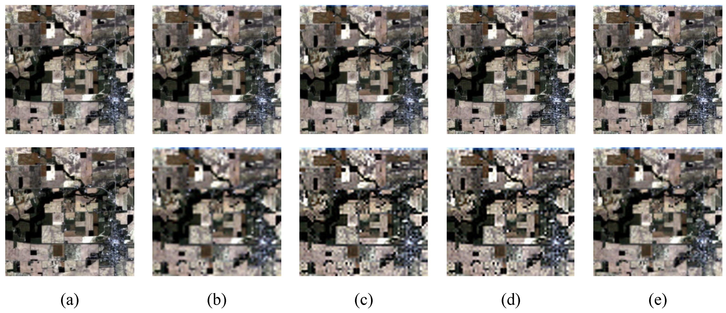
4.1. Experiments on Simulated Datasets

Two datasets are used in simulated experiments to compare the performance of our proposed method with spatial resolution enhancement methods and spectral resolution enhancement methods, respectively. Both of simulated datasets Indian pines and Cuprite are acquired by AVIRIS sensor. The spatial resolution is 20 m and there are 224 spectral bands covering from 400 nm to 2500 nm. Indian pines dataset is captured over Northwest of Indiana, USA. Cuprite dataset is obtained over the Cuprite mine district in Nevada. Sub-scenes with the size of 256 × 256 are extracted in both Indian pines and Cuprite datasets. The spectral bands with serious noises and water vapor absorption are discarded, so 162 bands remained.

The above data is considered as ground truth HR HSI with high spectral- and spatial- resolution. Input LR MSI is generated by spatial down-sampling and spectral down-sampling, respectively. A Gaussian filter and a spatial down-sampling factor are applied for spatial down-sampling [49]. For Indian pines dataset and Cuprite dataset, spectral down-sampling is implemented using the given spectral response function between Landsat TM and AVIRIS. The simulated MSI is generated with uniform spectral response functions corresponding to Landsat TM bands 1-5 and 7, which cover the wavelength of 450-520, 520-600, 630-690, 760-900, 1550-1750, and 2080-2350 nm, respectively [17]. Spatial dictionary is trained by HR PAN image simulated by the bands of ground truth over the visible wavelength. The spatial resolutions of PAN image and ground truth HSI are the same. Spectral dictionary is learned from LR prior HSIs which are generated by spatially down-sampling different AVIRIS HSIs with the same spectral configuration as ground truth HSI. In the experiment on Indian pines, the prior HSIs are Moffett Field HSI and Cuprite HSI. While Indian pines and Moffett Field are treated as prior HSIs in the experiment on Cuprite dataset.

The input of our proposed method is a MSI with low spatial and spectral resolution, which should be the same as all of compared methods to make fair comparison. Several PAN-sharpening methods are exploited to compare the performance of spatial resolution enhancement. The result of our proposed method J-SpeSpaRE is the HSI with high spatial and spectral resolution, which should be spectrally degraded in the comparison of spatial enhancement.

Spatial assessment comparison on Indian pines dataset and Cuprite dataset are respectively presented in

Table 1. Spatial assessment of our proposed method and pan-sharpening methods on Indian pines dataset.

	GSA	Indusion	SparseFI	J-SpeSpaRE (After Spectral Degradation)
MPSNR	37.030	38.234	38.735	39.097
MSSIM	0.693	0.729	0.738	0.756
MFSIM	0.797	0.823	0.844	0.899
SAM	0.160	0.151	0.147	0.120
PD	7.874	6.350	5.192	4.318

and

Table 2. Spatial assessment of our proposed method and pan-sharpening methods on Cuprite dataset.

	GSA	Indusion	SparseFI	SpeSpaRE (After Spectral Degradation)
MPSNR	41.065	42.371	43.012	43.855
MSSIM	0.699	0.728	0.740	0.759
MFSIM	0.754	0.797	0.831	0.884
SAM	0.160	0.142	0.139	0.114
PD	8.347	6.468	5.703	4.911

. The best evaluations are listed in bold letters. The pan-sharpening methods GSA, Indusion and SparseFI are used to compare the performance of spatial resolution enhancement. From Table 1 to Table 2, MPSNR, MFSIM, and MSSIM represent the average values of all spectral bands while SAM denotes the average results of all pixels. It can be found from Table 1 and Table 2 that our proposed J-SpeSpaRE method achieves better spatial performance than other compared methods. GSA is a component substitution method and Indusion is a multi-resolution analysis method, both of which are conventional pan-sharpening techniques. SparseFI proves superior spatial enhancement results than GSA and Indusion due to the high spatial resolution dictionary trained by PAN image. However, spectral correlation and constraints are ignored in SparseFI, which leads to more spectral distortions than our proposed method. The proposed J-SpeSpaRE method can simultaneously improve spatial resolution and spectral resolution. PAN images are trained to generate spatial dictionary with high spatial resolution textures and structures via sparse representation, which is assumed to be benefited for acquiring high spatial resolution abundances. On the other hand, abundances are updated in each iteration by using the spectral dictionary trained in the previous iteration. Spectral dictionary and abundances are alternately solved to ensure more accurate spatial information and less spectral distortions. Except from the assessment evaluation, visual comparisons of each method on Indian pines dataset and Cuprite dataset are also represented in Figure 4 and Figure 5, where the reconstructed results are shown as red, green and blue bands. We found that all of the compared methods can recover high spatial resolution MSIs. However, spatial distortions exist in Indusion method and SparseFI method, while GSA method leads to serious spectral distortions and blurring. As indicated from Figure 4e and Figure 5e, our proposed method proves better visual performance and less distortions than other compared methods.

Spectral super-resolution methods are used to evaluate the effectiveness of spectral resolution enhancement. For fair comparison, the result of our proposed method J-SpeSpaRE should be spatially degraded. The spectral assessments on both Indian pines dataset and Cuprite dataset are listed in

Table 3. Spectral assessment of our proposed method and spectral resolution enhancement methods on Indian pines dataset.

	Arad	SREM	J-SpeSpaRE (After Spatial Degradation)
RMSE	4.872	4.548	4.230
SAM	0.230	0.211	0.209
MPSNR	33.682	34.177	34.802
CC	0.930	0.967	0.970

and

Table 4. Spectral assessment of our proposed method and spectral resolution enhancement methods on Cuprite dataset.

	Arad	SREM	J-SpeSpaRE (After Spatial Degradation)
RMSE	4.5372	4.1020	3.5989
SAM	0.245	0.216	0.191
MPSNR	35.936	37.294	37.997
CC	0.955	0.971	0.932

, respectively. The best evaluation results are written in bold letters. The compared spectral resolution enhancement methods include Arad and SREM. In Table 3 and Table 4, our proposed method achieves better or more competitive results than the compared methods. Figure 6 and Figure 7 show visual comparison of Indian pines dataset and Cuprite dataset, where the spectral enhancement results of band 550 nm, 750 nm, and 1500 nm are presented. Arad’s method is designed based on sparse representation framework where a high-resolution spectral dictionary is trained using hyperspectral priors. Spatial constraints are ignored in Arad’s method, so it suffers from serious spatial and spectral distortions. A transformation matrix between input MSI and the desired HSI is estimated in SREM method, where spatial correlation is not used because of the pixel by pixel processing. The proposed J-SpeSpaRE method shows superior comparison results than Arad’ method and SREM. Spatial observation model and spectral observation model are designed to acquire high spectral resolution dictionary and high spatial resolution abundances in an alternative approach. These two steps are used as constraint for each other, so spectral distortions are reduced, and spatial features are maintained.

4.2. Effectiveness of Joint Spatial and Spectral Enhancement Framework

In this paper, spectral- and spatial enhancement are implemented in a unified framework where spectral dictionary and abundances are iteratively solved to achieve a high resolution HSI from the input MSI with low spatial and low spectral resolutions.

To validate the effectiveness of the proposed joint spatial and spectral enhancement framework, the spatial evaluation values of PSNR and RMSE, as well as the spectral evaluation values of SAM in each iteration are given in Figure 8, where assessments on Indian pines dataset and Cuprite dataset are presented by blue solid curves and black dashed curves, respectively. From Figure 8, the reconstruction performance increases dramatically at the first and second iterations, and then improves very slowly when iterating. In this paper, 4 and 5 are the best iteration times for Indian pines dataset and Cuprite dataset, respectively. So, the increasing performance in each iteration indicates the superiority of the proposed joint spatial and spectral enhancement framework.

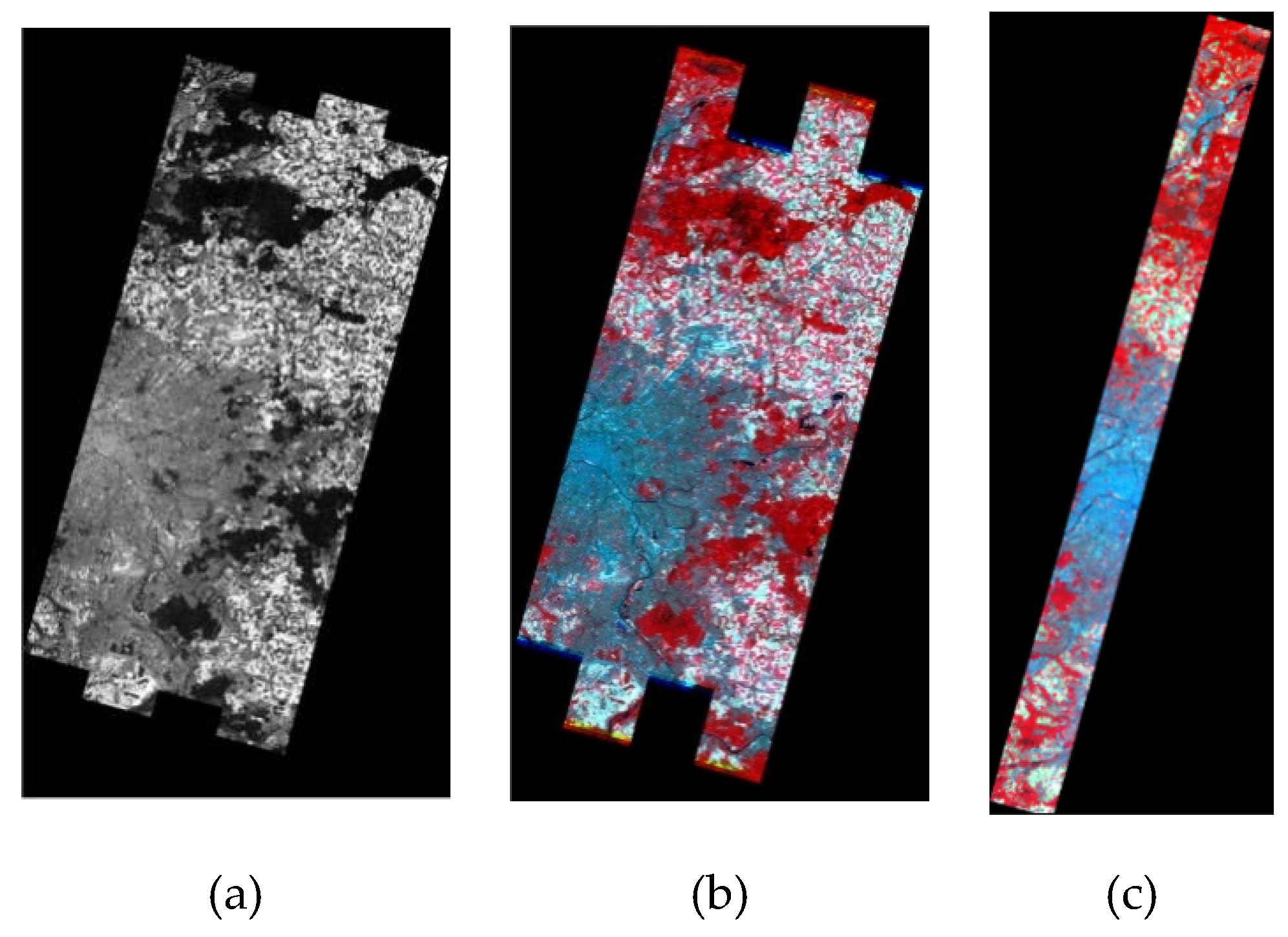
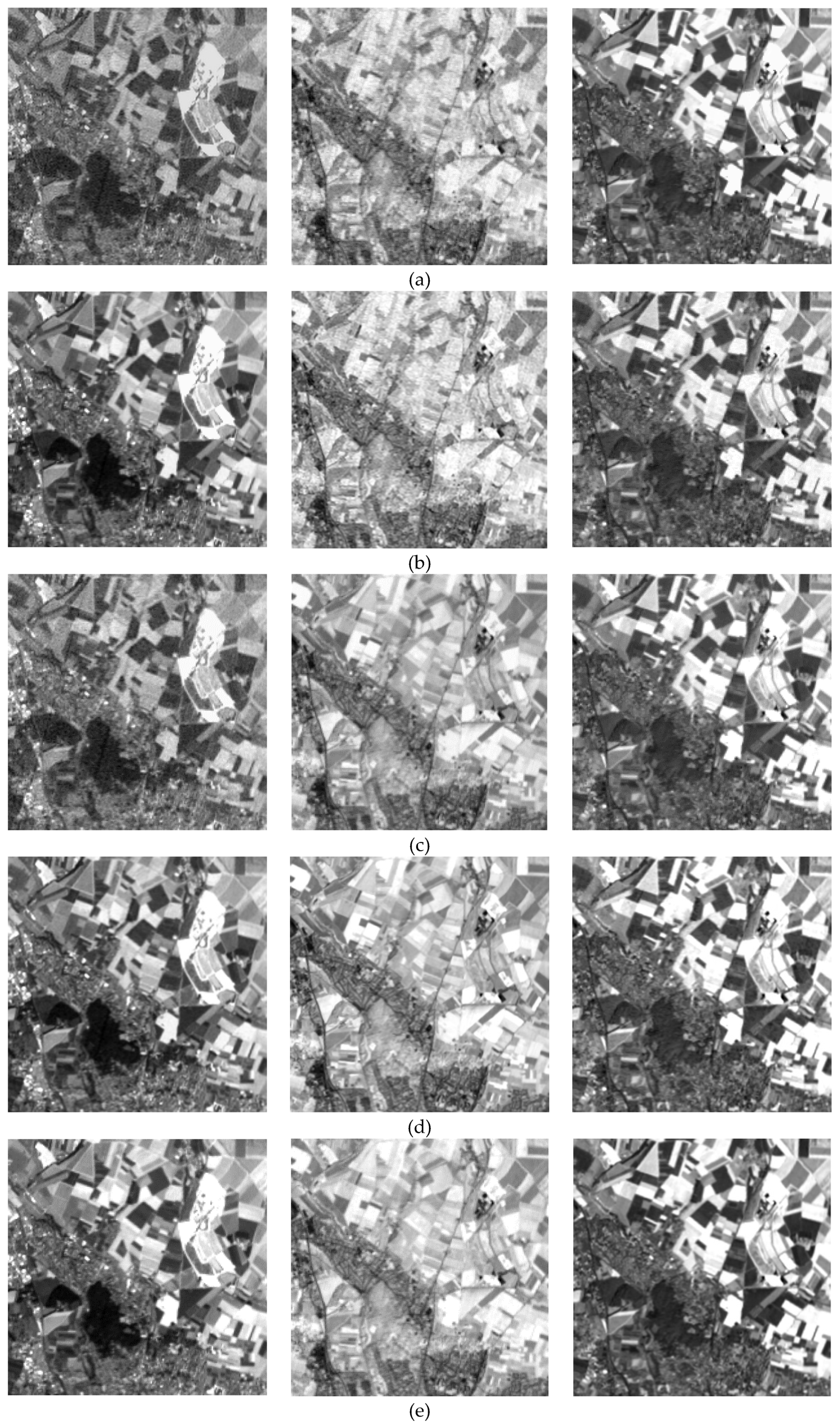
4.3. Experiment on Real Dataset

ALI/Hyperion real datasets captured by EO-1 satellite are applied to evaluate the performance of the proposed method. EO-1 satellite simultaneously carries hyperspectral Hyperion sensor and multispectral ALI sensor, where Hyperion sensor captures 242 hyperspectral bands and ALI sensor captures one PAN band and nine multispectral bands [50]. The spectral resolution of Hyperion image is 10 nm. The spatial resolutions of ALI image and Hyperion image are both 30 m. The spatial resolution of PAN image is 10 m. PAN image (10 m) and MSI (30 m) can be directly acquired to recover the corresponding HSI (10 m) using spatial dictionary trained from PAN image and spectral dictionary trained from prior HSIs (30 m) over various scenes. The selected Hyperion/ALI images are obtained in June of 2002 over the city of Paris, France. Figure 9a shows the PAN image, and RGB compositions of ALI and Hyperion images are presented in Figure 9b,c. The prior hyperspectral data used for training initial spectral dictionary are Hyperion hyperspectral data captured over the cities of Berlin, Germany, and Xi’an, China. Atmospheric correction and registration are firstly performed. Fast Line-of-sight Atmospheric Analysis in ENVI 5.3 is used for atmospheric correction [24]. The polynomial algorithm is exploited to register Hyperion image to ALI image by selecting more than 50 pairs of tie points.

Combinations of state-of-the-art spatial resolution enhancement methods and spectral resolution enhancement methods are used in this section to compare with our proposed J-SpeSpaRE method. Figure 10 shows the RGB compositions of the proposed method and all of combined methods. The input is ALI MSI with spatial resolution of 30 m, spatial resolution enhancement method (Indusion or SparseFI) and spectral resolution enhancement method (Arad’s method or SREM method) are sequentially performed to achieve the recovered Hyperion HSI with spatial resolution of 10 m, which is used to compare with the reconstruction result of our proposed J-SpeSpaRE method. There are four combinations of spatial resolution enhancement methods and spectral resolution enhancement methods, which are denoted as Indusion+Arad, Indusion+SREM, SparseFI+Arad and SparseFI+SREM. The high-resolution hyperspectral ground truth is not available in real case, so only the overlapped regions of ALI and Hyperion images could be used to evaluate the reconstruction performance of all compared methods. Comparisons of sub-scenes at band 550 nm, band 900 nm, and band 1,600 nm are presented in Figure 11.

From visual comparison, our proposed joint spatial and spectral enhancement method achieves better results than other combined methods. Clearer boundaries and less color distortions exist in our method, which proves the effectiveness of simultaneous improvement in the spatial and spectral domain. In the compared combination methods, the artifacts and errors are transformed from spatial enhancement to spectral enhancement through the sequential approach. The Indusion+Arad method and Indusion+SREM method suffer from spatial blurring and distortions due to the drawback of Indusion method. SREM method takes advantage of underlying spectral materials so less spectral distortions are presented in the combination SparseFI+SREM method. Our proposed method obtains overall better results than other compared methods, exploits spectral observation model and spatial observation model, and also unifies them into a joint framework to iteratively solve spectral dictionary and abundances. Spectral and spectral resolutions are simultaneously improved with less errors and distortions.

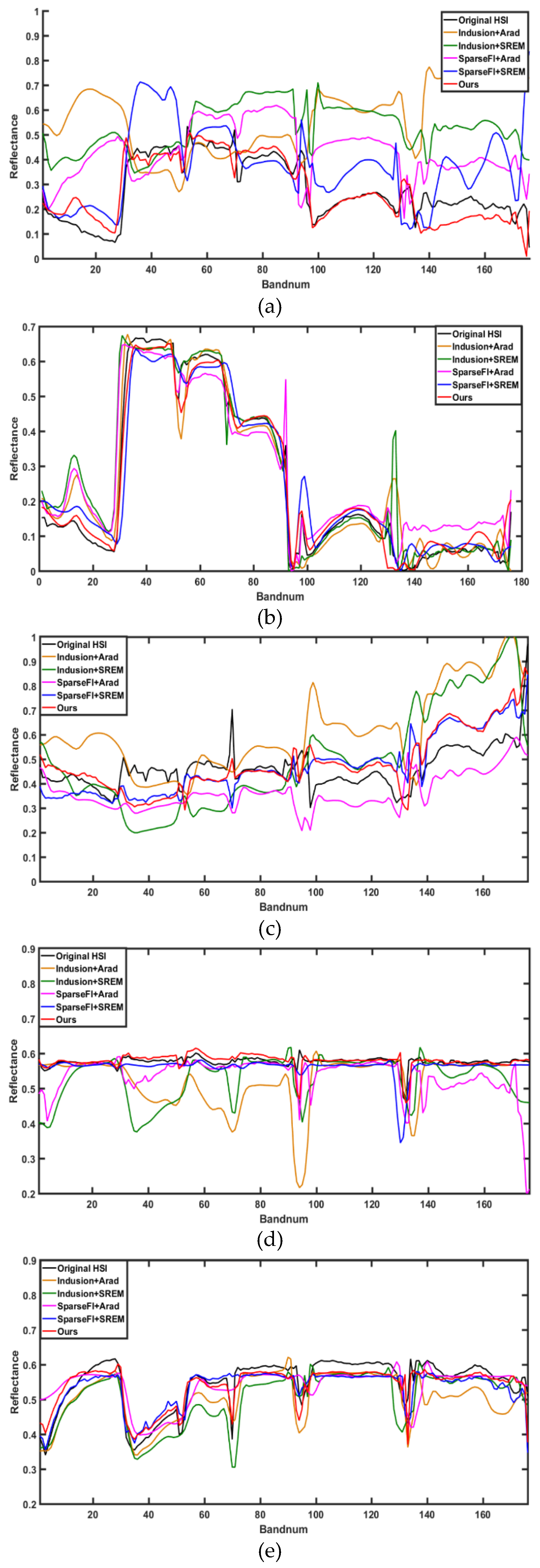
4.4. Spectral Unmixing on Real Dataset

Spectral unmixing is applied to the recovered HR HSIs of the real dataset to evaluate the performance of the proposed method. Endmembers indicate spectral reflectance of each landscape and abundances prove proportion of each endmember. VCA [51] is utilized as endmember extraction algorithm and SUnSAL [28] is exploited for abundances estimation. The sub-scenes in Figure 11 are used in spectral unmixing of the proposed and the methods for comparison. The false color composite is given in Figure 12 where five landscapes (Woods, Lawn, Residence, Sand land, and Crop land) are selected to evaluate accuracy of spectral signatures. Spectral unmixing result of the original LR Hyperion Paris HSI is also given to verify effectiveness of the proposed joint spatial and spectral resolution enhancement method.

Figure 13 shows that the reflectance of the five selected endmembers of all compared methods (Indusion+Arad, Indusion+SREM, SparseFI+Arad, and SparseFI+SREM) and the proposed method. The abundances maps of each endmember are also listed in Figure 14. In Figure 13, our proposed method achieves better performance of endmember extraction than other combined methods. Spectral reflectance of our proposed method has the lowest difference from the original HSI. More accurate spectral endmembers can be extracted after improving spatial- and spectral- resolution simultaneously than applying spatial enhancement and spectral enhancement step by step. Figure 14 shows the superiority of spatial information achieved by our method, where high spatial resolution abundance maps have more clear structures, sharp edges and spatial details than other combined methods. Reliable spectral signatures and high-resolution spatial features can be acquired through joint spatial- and spectral- resolution enhancement to verify the accuracy and effectiveness of the proposed method.

5. Conclusions

This paper proposes a joint spatial-spectral resolution enhancement algorithm based on spectral factorization and spatial sparsity to achieve an HR HSI from an input LR MSI. Spectral and spatial observation models are formulated to describe spectral and spatial relationship schemes between the input MSI and the desired HSI. Virtual intermediate variables, LSpaHSpe and HSpaLSpe, are introduced to make more comprehensive descriptions in spectral and spatial observation models which are used to respectively solve high spectral resolution dictionary and high spatial resolution abundances. Spectral dictionary can be trained by adapting prior LSpaHSpe HSIs, and abundances are obtained by using sparse coefficients as spatial constraint. A spatial observation model and a spectral observation model are unified into a joint framework to alternately solve spectral dictionary and abundances. These two steps can be used as constraints for each other and finally achieve the result of joint spatial-spectral enhancement without solving the virtual intermediate variables. The proposed joint spatial-spectral enhancement framework overcomes the drawback of a sequential implementation of spatial improvement and spectral enhancement steps to achieve more accurate reconstruction results and low distortions.

References

1. Yang, J.; Zhao, Y.Q.; Chan, J.C.W. Learning and transferring deep joint spectral-spatial features for hyperspectral classification. IEEE Trans. Geosci. Remote Sens. 2017, 55, 4729–4742. [Google Scholar] [CrossRef]
2. Zhang, Y.; Du, B.; Zhang, L.; Liu, T. Joint sparse representation and multitask learning for hyperspectral target detection. IEEE Trans. Geosci. Remote Sens. 2017, 55, 894–906. [Google Scholar] [CrossRef]
3. Lorente, D.; Aleixos, N.; Gómez-Sanchis, J.; Cubero, S.; García-Navarrete, O.L.; Blasco, J. Recent advances and applications of hyperspectral imaging for fruit and vegetable quality assessment. Food Bioprocess Technol. 2012, 5, 1121–1142. [Google Scholar] [CrossRef]
4. Yokoya, N.; Chan, J.C.W.; Segl, K. Potential of resolution-enhanced hyperspectral data for mineral mapping using simulated EnMAP and Sentinel-2 images. Remote Sens. 2016, 8, 172. [Google Scholar] [CrossRef] [Green Version]
5. Yi, C.; Zhao, Y.Q.; Chan, J.C.W. Hyperspectral image superresolution based on spatial and spectral correlation fusion. IEEE Trans. Geosci. Remote Sens. 2018, 56, 4165–4177. [Google Scholar] [CrossRef]
6. Yang, J.; Zhao, Y.Q.; Chan, J.C.W.; Xiao, L. A Multi-Scale Wavelet 3D-CNN for Hyperspectral Image Super-Resolution. Remote Sens. 2019, 11, 1557. [Google Scholar] [CrossRef] [Green Version]
7. Loncan, L.; De Almeida, L.B.; Bioucas-Dias, J.M.; Briottet, X.; Chanussot, J.; Dobigeon, N.; Fabre, S.; Liao, W.; Licciardi, G.A.; Simoes, M.; et al. Hyperspectral pansharpening: A review. IEEE Geosci. Remote Sens. Mag. 2015, 3, 27–46. [Google Scholar] [CrossRef] [Green Version]
8. Dalla Mura, M.; Vivone, G.; Restaino, R.; Addesso, P.; Chanussot, J. Global and local Gram-Schmidt methods for hyperspectral pansharpening. In Proceedings of the IEEE International Geoscience and Remote Sensing Symposium, Milan, Italy, 26–31 July 2015; pp. 37–40. [Google Scholar]
9. Licciardi, G.A.; Khan, M.M.; Chanussot, J.; Montanvert, A.; Condat, L.; Jutten, C. Fusion of hyperspectral and panchromatic images using multiresolution analysis and nonlinear PCA band reduction. EURASIP J. Adv. Signal Process. 2012, 1, 207. [Google Scholar] [CrossRef]
10. Yang, S.; Zhang, K.; Wang, M. Learning low-rank decomposition for pan-sharpening with spatial- spectral offsets. IEEE Trans. Neural Netw. Learn. Syst. 2017, 20, 3647–3657. [Google Scholar]
11. Yi, C.; Zhao, Y.Q.; Yang, J.; Chan, J.C.W.; Kong, S.G. Joint hyperspectral superresolution and unmixing with interactive feedback. IEEE Trans. Geosci. Remote Sens. 2017, 55, 3823–3834. [Google Scholar] [CrossRef]
12. Wei, Y.; Yuan, Q.; Shen, H.; Zhang, L. Boosting the Accuracy of multispectral image pansharpening by learning a deep residual network. IEEE Geosci. Remote Sens. Lett. 2017, 14, 1795–1799. [Google Scholar] [CrossRef] [Green Version]
13. Yuan, Q.; Wei, Y.; Meng, X.; Shen, H.; Zhang, L. A multiscale and multidepth convolutional neural network for remote sensing imagery pan-sharpening. IEEE J. Sel. Top. Appl. Earth Obs. Remote Sens. 2018, 11, 978–989. [Google Scholar] [CrossRef] [Green Version]
14. Chan, R.H.; Chan, T.F.; Shen, L.; Shen, Z. Wavelet algorithms for high-resolution image reconstruction. SIAM J. Sci. Comput. 2003, 24, 1408–1432. [Google Scholar] [CrossRef]
15. Eismann, M.T.; Hardie, R.C. Hyperspectral resolution enhancement using high-resolution multispectral imagery with arbitrary response functions. IEEE Trans. Geosci. Remote Sens. 2005, 43, 455–465. [Google Scholar] [CrossRef]
16. Yokoya, N.; Grohnfeldt, C.; Chanussot, J. Hyperspectral and multispectral data fusion: A comparative review of the recent literature. IEEE Geosci. Remote Sens. Mag. 2017, 5, 29–56. [Google Scholar] [CrossRef]
17. Yokoya, N.; Yairi, T.; Iwasaki, A. Coupled nonnegative matrix factorization unmixing for hyperspectral and multispectral data fusion. IEEE Trans. Geosci. Remote Sens. 2012, 50, 528–537. [Google Scholar] [CrossRef]
18. Akhtar, N.; Shafait, F.; Mian, A. Bayesian sparse representation for hyperspectral image super resolution. In Proceedings of the 2015 IEEE Conference on Computer Vision and Pattern Recognition (CVPR), Boston, MA, USA, 7–12 June 2015; pp. 3631–3640. [Google Scholar]
19. Dong, W.; Fu, F.; Shi, G.; Cao, X.; Wu, J.; Li, G.; Li, X. Hyperspectral image super-resolution via non-negative structured sparse representation. IEEE Trans. Image Process. 2016, 25, 2337–2352. [Google Scholar] [CrossRef]
20. Yi, C.; Zhao, Y.Q.; Chan, J.C.-W. Spectral super-resolution for multispectral image based on spectral improvement strategy and spatial preservation strategy. IEEE Trans. Geosci. Remote Sens. 2019, 57, 9010–9024. [Google Scholar] [CrossRef]
21. Chi, C.; Yoo, H.; Ben-Ezra, M. Multi-spectral imaging by optimized wide band illumination. Int. J. Comput. Vis. 2010, 86, 140. [Google Scholar] [CrossRef]
22. Gat, N. Imaging spectroscopy using tunable filters: A review. Proc. SPIE 2000, 4056, 50–64. [Google Scholar]
23. Oh, S.W.; Brown, M.S.; Pollefeys, M.; Kim, S.J. Do it yourself hyperspectral imaging with everyday digital cameras. In Proceedings of the 2016 IEEE Conference on Computer Vision and Pattern Recognition (CVPR), Las Vegas, NV, USA, 27–30 June 2016; pp. 2461–2469. [Google Scholar]
24. Sun, X.; Zhang, L.; Yang, H.; Wu, T.; Cen, Y.; Guo, Y. Enhancement of spectral resolution for remotely sensed multispectral image. IEEE J. Sel. Top. Appl. Earth Obs. Remote Sens. 2015, 8, 2198–2211. [Google Scholar] [CrossRef]
25. Arad, B.; Ben-Shahar, O. Sparse recovery of hyperspectral signal from natural RGB images. In Computer Vision—ECCV 2016; Springer: Cham, Switzerland, 2016; pp. 19–34. [Google Scholar]
26. Wu, J.; Aeschbacher, J.; Timofte, R. In defense of shallow learned spectral reconstruction from RGB images. In Proceedings of the 2017 IEEE International Conference on Computer Vision Workshops (ICCVW), Venice, Italy, 22–29 October 2017; pp. 471–479. [Google Scholar]
27. Galliani, S.; Lanaras, C.; Marmanis, D.; Baltsavias, E.; Schindler, K. Learned Spectral Super-Resolution. arXiv 2017, arXiv:1703.09470. Available online: https://arxiv.org/abs/1703.09470 (accessed on 28 March 2017).
28. Bioucas-Dias, J.M.; Plaza, A.; Dobigeon, N.; Parente, M.; Du, Q.; Gader, P.; Chanussot, J. Hyperspectral unmixing overview: Geometrical, statistical, and sparse regression-based approaches. IEEE J. Sel. Top. Appl. Earth Obs. Remote Sens. 2012, 5, 354–379. [Google Scholar] [CrossRef] [Green Version]
29. Chakrabarti, A.; Zickler, T. Statistics of real-world hyperspectral images. In Proceedings of the IEEE Conference on Vision Pattern Recognit (CVPR) 2011, Providence, RI, USA, 20–25 June 2011; pp. 193–200. [Google Scholar]
30. Zhu, X.X.; Bamler, R. A sparse image fusion algorithm with application to pan-sharpening. IEEE Trans. Geosci. Remote Sens. 2013, 51, 2827–2836. [Google Scholar] [CrossRef]
31. Xue, J.; Zhao, Y.; Liao, W.; Chan, J.C.W. Nonlocal tensor sparse representation and low-rank regularization for hyperspectral image compressive sensing reconstruction. Remote Sens. 2019, 11, 193. [Google Scholar] [CrossRef] [Green Version]
32. Keshava, N.; Mustard, J.F. Spectral unmixing. IEEE Signal Process. Mag. 2002, 19, 44–57. [Google Scholar] [CrossRef]
33. Akhtar, N.; Shafait, F.; Mian, A. Sparse spatio-spectral representation for hyperspectral image super-resolution. In Computer Vision; Springer: Cham, Switzerland, 2014; pp. 63–78. [Google Scholar]
34. Zhao, Y.-Q.; Yang, J. Hyperspectral image denoising via sparse representation and low-rank constraint. IEEE Trans. Geosci. Remote Sens. 2014, 53, 296–308. [Google Scholar] [CrossRef]
35. Zhu, X.X.; Grohnfeldt, C.; Bamler, R. Exploiting joint sparsity for pansharpening: The J-SparseFI algorithm. IEEE Trans. Geosci. Remote Sens. 2016, 54, 2664–2681. [Google Scholar] [CrossRef] [Green Version]
36. Aharon, M.; Elad, M.; Bruckstein, A. K-SVD: An algorithm for designing overcomplete dictionaries for sparse representation. IEEE Trans. Signal Process. 2006, 54, 4311–4322. [Google Scholar] [CrossRef]
37. Afonso, M.V.; Bioucas-Dias, J.M.; Figueiredo, M.A.T. An augmented Lagrangian approach to the constrained optimization formulation of imaging inverse problems. IEEE Trans. Image Process. 2011, 20, 681–695. [Google Scholar] [CrossRef] [PubMed] [Green Version]
38. Boyd, S.; Parikh, N.; Chu, E.; Peleato, B.; Eckstein, J. Distributed optimization and statistical learning via the alternating direction method of multipliers. Found. Trends Mach. Learn. 2011, 3, 1–122. [Google Scholar] [CrossRef]
39. Daubechies, I.; Defrise, M.; De Mol, C. An iterative thresholding algorithm for linear inverse problems with a sparsity constraint. Commun. Pure Appl. Math. 2004, 57, 1413–1457. [Google Scholar] [CrossRef] [Green Version]
40. Friedman, J.; Hastie, T.; Höfling, H.; Tibshirani, R. Pathwise coordinate optimization. Ann. Appl. Statist. 2007, 1, 302–332. [Google Scholar] [CrossRef] [Green Version]
41. Donoho, D.L. For most large underdetermined systems of equations, the minimal 1-norm near-solution approximates the sparsest nearsolution. Commun. Pure Appl. Math. 2006, 59, 907–934. [Google Scholar] [CrossRef]
42. Golub, G.H.; Van Loan, C.F. Matrix Computations; The Johns Hopkins University Press: Baltimore, MD, USA, 1983. [Google Scholar]
43. Aiazzi, B.; Baronti, S.; Selva, M. Improving Component Substitution Pansharpening through Multivariate Regression of MS $ + $Pan Data. IEEE Trans. Geosci. Remote Sens. 2007, 45, 3230–3239. [Google Scholar] [CrossRef]
44. Khan, M.M.; Chanussot, J.; Condat, L.; Montanvert, A. Indusion: Fusion of Multispectral and Panchromatic Images Using the Induction Scaling Technique. IEEE Geosci. Remote Sens. Lett. 2008, 5, 98–102. [Google Scholar] [CrossRef] [Green Version]
45. Xue, J.; Zhao, Y.; Liao, W.; Chan, J.C.W. Nonlocal Low-Rank Regularized Tensor Decomposition for Hyperspectral Image Denoising. IEEE Trans. Geos. Remote Sens. 2019, 57, 5174–5189. [Google Scholar] [CrossRef]
46. Wang, Z.; Bovik, A.C.; Sheikh, H.R.; Simoncelli, E.P. Image quality assessment: From error visibility to structural similarity. IEEE Trans. Image Process. 2004, 13, 600–612. [Google Scholar] [CrossRef] [Green Version]
47. Lanaras, C.; Baltsavias, E.; Schindler, K.K. Hyperspectral Super-Resolution with Spectral Unmixing Constraints. Remote Sens. 2017, 9, 1196. [Google Scholar] [CrossRef] [Green Version]
48. Wald, L. Data fusion. In Definitions and Architectures—Fusion of Images of Different Spatial Resolutions; Ecole de Mines de Paris: Paris, France, 2002. [Google Scholar]
49. Zhang, L.; Wei, W.; Bai, C.; Gao, Y.; Zhang, Y. Exploiting clustering manifold structure for hyperspectral imagery super-resolution. IEEE Trans. Image Process. 2018, 27, 5969–5982. [Google Scholar] [CrossRef]
50. Folkman, M.A.; Pearlman, J.; Liao, L.B.; Jarecke, P.J. EO-1/hyperion hyperspectral imager design, development, characterization, and calibration. Proc. SPIE 2001, 4151, 40–51. [Google Scholar]
51. Ma, W.K.; Bioucas-Dias, J.M.; Chan, T.H.; Gillis, N.; Gader, P.; Plaza, A.J.; Chi, C.Y. A signal processing perspective on hyperspectral unmixing. IEEE Signal Process. Mag. 2014, 31, 67–81. [Google Scholar] [CrossRef] [Green Version]
Figure 1. The framework of the proposed method.
Remotesensing 12 00993 g001
Figure 2. A spatial observation model.
Remotesensing 12 00993 g002
Figure 3. A spectral observation model.
Remotesensing 12 00993 g003
Figure 4. Spatial resolution enhancement comparison on Indian pines dataset, from top to bottom are the comparison with down-sampling factor of 2 and 4. (a) Reference HRI, spatial resolution enhancement results of (b) GSA method, (c) Indusion method, (d) SparseFI method and (e) Proposed J-SpeSpaRE method (after spectral degradation).
Remotesensing 12 00993 g004
Figure 5. Spatial resolution enhancement comparison on Cuprite dataset, from top to bottom are the comparison with down-sampling factor of 2 and 4. (a) Reference HRI, spatial resolution enhancement results of (b) GSA method, (c) Indusion method, (d) SparseFI method and (e) Proposed J-SpeSpaRE method (after spectral degradation).
Remotesensing 12 00993 g005
Figure 6. Spectral resolution enhancement comparison on Indian pines dataset, from top to bottom are the comparison of band 550 nm, 750 nm, and 1500 nm. (a) Reference HRI, spectral resolution enhancement results of (b) Arad method, (c) spectral resolution enhancement method (SREM) method, (d) Proposed J-SpeSpaRE method (after spatial degradation).
Remotesensing 12 00993 g006
Figure 7. Spectral resolution enhancement comparison on Cuprite dataset, from top to bottom denote band 550 nm, 750 nm, and 1500 nm. (a) Reference HRI, spectral resolution enhancement results of (b) Arad method, (c) SREM method, (d) Proposed J-SpeSpaRE method (after spatial degradation).
Remotesensing 12 00993 g007
Figure 8. Assessment values of each iteration on both Indian pines dataset and Cuprite dataset (a) Peak Signal-to-Noise Ratio (PSNR), (b) Root-Mean-Square Error (RMSE), and (c) Spectral Angle Mapper (SAM).
Remotesensing 12 00993 g008aRemotesensing 12 00993 g008b
Figure 9. ALI PAN image (a), RGB compositions of ALI MSI (b) and Hyperion HSI over Paris (c).
Remotesensing 12 00993 g009
Figure 10. RGB compositions of (a) Indusion+Arad method, (b) Indusion+SREM method, (c) SparseFI+Arad method, (d) SparseFI+SREM method, (e) Proposed J-SpeSpaRE method.
Remotesensing 12 00993 g010
Figure 11. Comparison of sub-scenes in real dataset at band 550nm, band 900 nm, and band 1,600 nm (from left to right) (a) Indusion+Arad method, (b) Indusion+SREM method, (c) SparseFI+Arad method, (d) SparseFI+SREM method, (e) our proposed J-SpeSpaRE method.
Remotesensing 12 00993 g011
Figure 12. False color composite of the Hyperion sub-scene and five selected landscapes.
Remotesensing 12 00993 g012
Figure 13. Comparison of reflectance of five selected endmembers in real dataset, (a) Wood, (b) Lawn, (c) Residence, (d) Sand land, and (e) Crop land.
Remotesensing 12 00993 g013
Figure 14. Comparison of abundance maps of the five selected endmembers in real dataset, (a) Original HSI, (b) Indusion+Arad, (c) Indusion+SREM, (d) SparseFI+Arad, (e) SparseFI+SREM, and (f) Our method.
Remotesensing 12 00993 g014