Article

Application of Convolutional Neural Network on Lei Bamboo Above-Ground-Biomass (AGB) Estimation Using Worldview-2

1
State Key Laboratory of Subtropical Silviculture, Zhejiang A & F University, Hangzhou 311300, China
2
Key Laboratory of Carbon Cycling in Forest Ecosystems and Carbon Sequestration of Zhejiang Province, Zhejiang A & F University, Hangzhou 311300, China
3
School of Environmental and Resources Science, Zhejiang A & F University, Hangzhou 311300, China
4
The College of Forestry, Beijing Forestry University, Beijing 100083, China
*
Author to whom correspondence should be addressed.
Remote Sens. 2020, 12(6), 958; https://doi.org/10.3390/rs12060958
Submission received: 9 February 2020 / Revised: 7 March 2020 / Accepted: 11 March 2020 / Published: 16 March 2020
(This article belongs to the Section Remote Sensing in Agriculture and Vegetation)

Abstract

:
Above-ground biomass (AGB) directly relates to the productivity of forests. Precisely, AGB mapping for regional forests based on very high resolution (VHR) imagery is widely needed for evaluation of productivity. However, the diversity of variables and algorithms and the difficulties inherent in high resolution optical imagery make it complex. In this paper, we explored the potentials of the state-of-art algorithm convolutional neural networks (CNNs), which are widely used for its high-level representation, but rarely applied for AGB estimation. Four experiments were carried out to compare the performance of CNNs and other state-of-art Machine Learning (ML) algorithms: (1) performance of CNN using bands, (2) performance of Random Forest (RF), support vector regression (SVR), artificial neural network (ANN) on bands, and vegetation indices (VIs). (3) Performance of RF, SVR, and ANN on gray-level co-occurrence matrices (GLCM), and exploratory spatial data analysis (ESDA), and (4) performance of RF, SVR, and ANN based on all combined data and ESDA+VIs. CNNs reached satisfactory results (with R2 = 0.943) even with limited input variables (i.e., only bands). In comparison, RF and SVR with elaborately designed data obtained slightly better accuracy than CNN. For examples, RF based on GLCM textures reached an R2 of 0.979 and RF based on all combined data reached a close R2 of 0.974. However, the results of ANN were much worse (with the best R2 of 0.885).

1. Introduction

The above ground biomass (AGB) of forests is related to the productivity of forests, carbon cycle, and habitation in terrestrial ecosystems [1,2]. Evaluation of biomass is crucial for monitoring and estimating forest quality [3,4]. Moreover, accurate estimation of biomass could reduce the uncertainty in monitoring global climate changes [5,6,7,8,9]. There are several methods used to evaluate the AGB of forests. Directly calculating biomass by cutting down and weighing the whole tree is accurate but destructive and too expensive. A more prevalent method is cutting down some trees as samples to construct an allometric model [10], which would be used to estimate the AGB of other trees. Recent field surveys exclusively record key growth factors, such as diameters at breast height (DBH), average tree heights, total tree numbers, and tree species, which save lots of time and resources. However, obtaining forest inventory data of large areas using allometric models is still time-consuming and labor-intensive.
Remote sensing (RS) technology provides an alternative for biomass evaluation [11]. RS data covers large areas and is available for temporal analysis. However, previous works have shown that due to the variety of RS data sources and the condition of the target area, there is no paradigm to apply RS on biomass estimation. Light Detection and Ranging (LiDAR) and radar do have many advantages [12,13] because tree height and the crown can be measured and modeled. Literature has suggested that LiDAR, especially airborne LiDAR data, are more prevailing and reliable [14]. However, limited availability constrains the application of LiDAR. Medium and low spatial resolution spectral images, such as Landsat TM (Thematic mapper), Landsat OLI (Operational Land Imager) imageryand the Moderate Resolution Imaging Spectroradiometer (MODIS) products, have been investigated for decades since spectrums indirectly relate to plant growth status [2,7,15,16]. Scholars used these data to reveal climate change and environmental shifts at impressive scales [17,18].
Nowadays, most state-of-the-art satellites are equipped with sensors of hyperspectral or high resolution indicating the increasing demands for precise RS products. Very high spatial resolution image (VHSR) provides sufficient spatial information and relatively valuable spectrums [19]. For instance, convenient Unmanned Aerial Vehicles (UAV) capture large amounts of images all around the world [12]. VHSR satellite images, such as worldview, QuickBird [20], if well utilized, are valuable data sources for precise AGB mapping. However, VHSR images, both from the airborne and spaceborne, have some drawbacks, such as within-class spectrum variance and lack of information about the vertical structure of forests.
There are several RS variables including raw bands, vegetation indices (VIs), and spatial textures, proved to be correlated with AGB [21,22,23]. Traditionally defined vegetation indices (VIs) such as Difference Vegetation Index (DVI), and Normalized Difference Vegetation Index (NDVI) are sensitive to vegetable growth status. However, bands and VIs face the “saturation” problem [19,22]. Spatial textures [24,25] aids VHSR tasks because radiational distortion that dramatically impacts optical spectrums does not impact textures very much [11]. Generally, spatial textures can be classified into three types: (1) features based on local variation measures, (2) features based on second-order statistics, such as gray-level co-occurrence matrices (GLCM), and (3) features based on spatial statistics (such as semi-variance textures) [26]. Especially, GLCM textures are vastly prevalent among RS studies including classification and forest parameters retrieve [1,11,19,24,25,26,27,28,29,30].
However, RS variables are naturally of high dimension. The algorithms used to connect the inputs and targets are crucial in this context. Traditional linear and nonlinear functions such as linear, power or logical regression models have been proven limited [31] for biomass retrieve using spectrums and other ancillary information, especially high resolution ones, for that they assume the given data come from a known statistic distribution [13,14,32]. However, most ML methods do not require such an assumption, though normally distributed data turn out to perform better. For instances, artificial neural network ANN [33], RF [34,35,36,37], and support vector regression (SVR) [38,39] are very popular these years. The explanations of these algorithms are shown in the Materials and Methods section.
To the best of our knowledge, convolutional neural networks (CNNs), though widely investigated and highly praised for classification tasks [40], are rarely used for AGB estimation. Drawbacks inherent in CNNs and VHSR images constrain the use of CNNs for biomass estimation: spatial heterogeneity and, especially, the lack of sufficient training samples [41]. Unlike classification tasks that samples could be obtained less costly, AGB samples are relatively expensive. Distant pixels are weakly related and maybe overweight on CNN due to the lack of samples (overfitting). The potential of using CNN is beyond doubt, given how dramatically texture information improves AGB estimation. The assumptions are: (1) spatial information highly relates to AGB in VHSR images and (2) CNNs could, to some extent, extract spatial information based on training samples [42,43]. Thus, in this study, we take CNN as one of the chosen methods for AGB estimation in motivation for exploring its potential.
In conclusion, the question is how all the variables and algorithms impact the estimation of VHSR AGB estimation. The objectives of this paper are: (1) explore the potential of CNN for VHSR imagery AGB estimation, (2) test state-of-art ML algorithms and compare with CNN, and (3) test the performance of widely applied variables, including VIs, GLCM textures, and exploratory spatial data analysis (ESDA) textures.

2. Materials and Methods

2.1. Study Area and Field Survey

The study area is located in Taihuyuan, Zhejiang province, South China (Figure 1). The area has a monsoon-type climate, warm and humid, with sufficient sunshine, abundant rainfall. Four seasons are distinctive. The average temperature of a year is 16.4 °C and the total precipitation for one year is 1628.6 mm. Vegetation is mainly composed of broadleaf forests, coniferous (mainly Cunninghamia lanceolate and Pinus massoniana Lamb), and lei bamboo (Phyllostachys praecox C. D. Chu et C. S. Chao ’Prevernalis’) forests. Lei bamboos are important economic crops that cover large areas inside the study area. Residents pay a lot of attention to the intensive cultivation of lei bamboo forests.
The field survey (Figure 1) was carried out in July 2019, including 45 plots. For each plot, a 5 squared area (25 m2) was placed to cover a homogenous area of lei bamboos, inside which the number of trees and average DBH were measured. An Unistrong mobile GIS was used to determine the precise location of every plot at the center. The Global Positioning System (GPS) accuracy is 2–5 m, based on one satellite, and would be improved to 1–3 m based on Satellite-Based Augmentation System (SBAS). The points were further used to extract features from satellite imagery.
Allometric models are critical in preparing samples for RS-based biomass estimates. In this study, we took the allometric model constructed in the same area for lei bamboo forests [44,45]. The AGB (Kg) of a plot is calculated by:
AGB = N 0.1939 D 1.5654
where N indicates the number of trees and D is the average DBH.

2.2. Satellite Data

Since launch in October 2009, WorldView-2 has been in orbit and acquires data of a high spatial, as well as a higher spectral resolution, hopefully giving reliable sources for monitoring environmental changes [46]. In this study, the satellite data was obtained in July 2016. The image contains 4 bands, including Green (G, 450–510 nm), Blue (B, 510–581 nm), Red (R, 630–690 nm), Near-infrared red (NIR, 770–895 nm). The spatial resolution is 1.2 m. The image preprocessing including radiation correction and atmosphere correction was performed using ENVI 5.3. The radiance image was atmospherically corrected and transformed into canopy reflectance using the Fast Line-of-Sight Atmospheric Analysis of Spectral Hypercubes (FLAASH) algorithm.

2.3. Variables Extraction

In this section, descriptions of three chosen variables are given. The detailed formulas are shown in (Table 1); 45 points represented the precise locations of the 45 plots. For every point, 5 × 5 square-shaped pixels around the center point were obtained and every pixel was regarded as a separated sample. Therefore, the samples included 1125 pixels in total. However, a question must be pointed out. Given the spatial resolution of our satellite data is 1.2 m while the plot sizes are 5 m, the obtained pixels cover 6 × 6 m2—that is slightly larger than do real plots. Besides, some studies abandoned all the partly included pixels and computed the mean value of the pixels from each plot. The design of this experiment would be explained in Section 4.3. The samples were divided into training samples and testing samples with a ratio of 3:1. The pixels belong to one plot were only divided into training or testing set.
VIs, most of which are computed directly from bands, can reveal the growth status of vegetations. In our study, VIs included Difference Vegetation Index (DVI), Normalized Difference Vegetation Index (NDVI), Normalized Difference Water Index (NDWI), and Ratio Vegetation Index (RVI) [33]. The NDWI was included mainly for classification purpose.
Exploratory spatial data analysis (ESDA) represents a series of techniques that are used to statistically analyze spatial data and mine necessary knowledge of features’ spatial structure and correlation [47]. Information provided by ESDA is valuable for classification and spatial analysis [48,49]. However, few studies have taken ESDA into AGB estimation. In this study, we took two 3 indicators of ESDA into consideration: Moran’s I, Geary’s C, and G statistic [50,51,52,53]. Thus, for each band, there are 3 ESDA textures. We got 12 ESDA textures for each window size of ESDA.
The GLCM [54] is a tabulation of how often different combinations of pixel brightness values (grey levels) occur in an image. They are based on differences between pairs of pixels in a spatially defined relationship and consider all pixel pairs within the neighborhood. More information about GLCM could be found in [55,56]. GLCM textures have been proven to be vastly informative for high resolution AGB estimate [19,25,26]. Though are widely used, the window sizes of GLCM textures worth paying attention to. Especially, GLCM textures based VHRS would be much more informative than these based on high or middle resolution imagery. In our study, GLCM window sizes were set from 3 to 53 to explore the influence of spatial scales. For each window size, there were 4 bands, 4 directions and 8 kinds of GLCM textures Mean (MEA), Variance (VAR), Homogeneity (HOM), Contrast (CON), Dissimilarity (DIS), Entropy (ENT), Augular Second Moment (ASM), Correlation (COR). Therefore, we got 128 GLCM textures for each window size.

2.4. Machine Learning Algorithms

The relationships between biomass and RS variables are usually nonlinear. Using nonparametric models to estimate biomass in a data-driven manner is prevalent. However, it is hard to determine which ML algorithm is the best without experiment. Comparing different algorithms is helpful for revealing the relationships between biomass and RS variables [13]. Four ML models, including Convolutional neural networks (CNNs), Random forest (RF), Support vector regression (SVR), Artificial Neural Networks (ANNs), were applied to estimate AGB. Unless otherwise stated, every algorithm was run for 50 times to reduce the uncertainty that existed in algorithms and sample splits.

2.4.1. CNN

Convolutional neural networks (CNNs) in our study served as spatial information extractors. The formula of convolution [40] is given by:
m a p l , j x , y = f ( m h = 0 H l 1 w = 0 W l 1 k l , j . m h , w m a p ( l 1 ) ,   m ( x + h ) , ( y + w ) + b l , j )
where k l , j . m h , w is the value at the position (h, w) of the kernel connected to the mth feature map in the (l − 1)th layer, Hi and Wi are the height and width of the kernel, respectively, bl,j is the bias of the jth feature map in the lth layer, f(x) is an activation function.
The derivatives of the loss function with respect to parameters are computed based on the chain derivative rule along the computational graph during backward propagation. We denoted the gradient of a trainable parameter w with respect to loss as gradw. Based on gradw, we applied the Adam [60] algorithm as the optimizer, by which the learning rate changes adaptively during the training process. The formulas of the Adam algorithm are given by:
M 1 = β 1 × M 1 + ( 1 β 1 ) × g r a d w
M 2 = β 2 × M 2 + ( 1 β 2 ) × ( g r a d w ) 2
b 1 = M 1 1 β 1 t
b 2 = M 2 1 β 2 t
w = w b 1 × l r b 2 + ε
where M1 and M2 are the first and second momentum, while b1 and b2 are the amendments to M1 and M2 to avoid having a ‘big step’ at the beginning of the training. t is the number of training epochs. Other hyperparameters must be defined by empirical studies: β1 and β2 are the decay rates of the momentum, usually set as 0.9 and 0.999, respectively; lr is the learning rate, which is set as 3e-4; ε is a small number used to avoid the exception of being divided by 0.
In our study, CNN was designed as a simple structure to conduct more repeats to reduce the uncertainty of samples and test the inputs’ window sizes. For every pixel, the biomass of the pixel is estimated based on spatial and spectral properties from proximal pixels [26] as shown in Figure 2, or in other words, sliding windows. The CNN used included 8 convolutional layers and 2 linear fully connected layers at the end. Adam algorithm was used for optimization with a learning rate of 3e-4. The loss function was MSE (mean-squared error), the same as ANN. The activation function was Relu: f(x) = max(x, 0). The parameter settings of CNN were all the same over different inputs in our study.

2.4.2. RF

RF [61] is a state-of-art ensemble algorithm, which is widely applied for classification and regression for its robustness and understandable feature-selection procedures [12,23]. On the other hand, RF provides other appealing statistical properties, such as the useful internal estimates of error, correlation and variable importance [20]. RF constructs numerous regression trees to determine the final result by an average of all regression trees. RF is built up by these steps: (1) firstly, bootstrap is used to randomly select one sample of the training data with replacement. (2) Repeat step 1 until the number of selected samples is the same as the training data. This procedure is called bagging. Some samples may be picked up more than once, some may not be picked up at all. Around 37% of training data are not selected in a bagging. (3) A classification and Regression Tree (CART) is built upon the selected data in (2) without pruning. Several variables (n = mtry) are randomly selected to determine the best split of the node based on the Gini Impurity of all the variables, and (4) numerous trees (n = ntree) are put together and vote (average in regression) for final outputs. In this study, RF algorithm was carried out based on R [62] add-in package randomForest [63].
The classification map is obtained using an RF classifier. Bands, VIs, and 8 kinds of GLCM textures for 4 bands with window sizes of 3, 5, 7, 9, 11, 13 were included. In order to reduce the dimension of samples in the classification procedure, the mean values of the 4 direction (0°, 45°, 90°, 135°) of GLCM were calculated. Therefore, 4 bands, 4 VIs, and 192 GLCM textures (4 bands × 8 kinds × 6 window sizes) consisted of 200 variables in total. The samples were obtained by expert experience. 4000 pixels were randomly selected as samples for an RF classifier and were divided into training samples and testing samples with a ratio of 3:1. The optimal value of mtry in classification experiment was obtained by traversing all possible values and the ntree was set to 2000.
The AGB estimate based on the 1125 pixels we obtained. Variables were extracted and RF regression was used to construct models. AGB samples were randomly divided into training samples and testing samples with a ratio of 3:1 at each repeat. Due to the extensive computation in our study and the insensitiveness of RF to parameter settings, we took 1/3 of the number of variables as the value of mtry, as recommended by previous studies [63,64]. The ntree values of all repeats were set to 2000. Detailed parameters were listed in the Result section.

2.4.3. SVR

Support vector machine (SVM) [14] is a supervised non-parametric statistical learning technique; therefore, there is no assumption made on the underlying data distribution nor on the dimensions of the input space [38,65]. SVMs presented with a set of labeled data instances and the SVMs training algorithm aims to find a hyperplane that separates the groups of input data into a discrete predefined number of classes in a fashion consistent with the training examples. Besides, SVM is appealing for regression, denoted as SVR. Many excellent works apply SVR for RS tasks, such as retrieval of oceanic chlorophyll concentration [66], biomass estimation [14].
In our study, SVR algorithm was carried out based on R [62] and RBF kernel was used. The optimization of SVR mostly bases on C and ε, where C balances the minimization of errors and the regularization term and ε defines a loss-free tube around the calibration data where the deviation is not penalized [39]. SVR algorithm is sensitive to parameter settings. Therefore, for every feature set, the C and ε were tested at a range of values to determine the value that max the accuracies. Detailed parameters were listed in the Result section.

2.4.4. ANN

ANNs have been developed for decades. Standard ANNs have one input layer, one output layer, numerous hidden layers, and use activation functions such as Sigmoid, Relu, Tanh for non-linearization. Recently, new computer technology and the development of artificial intelligence make deeper and larger neural networks possible. For example, the dropout [67] algorithm could dramatically and efficiently reduce the risk of overfitting.
In our study, dropout and ormalization [68] were used for the improvement of the models. The ANN used included 9 hidden layers. Adam algorithm was used for optimization [60] with the learning rate of 3e-4. MSE (mean-squared error) was applied as the loss function. The activation function was Relu: f(x) = max(x, 0). The parameter settings of ANN were all the same over different input in our study.

2.5. Experiment Design

The flowchart of steps is shown in Figure 3. The experiments were designed as 5 parts: (1) classification map is produced using RF, (2) CNN was used to estimate AGB with bands as inputs, (3) RF, SVR, and ANN are individually applied on the widely applied variables, and (4) according to the performances of all these methods, several relatively better methods were selected for mapping AGB with land-use cover map. Three indicators were used to evaluate the performance of all the AGB estimation: coefficient of determination (R2), root mean squared error (RMSE), and relative RMSE (RMSEr).

3. Results

3.1. AGB Samples and Land Cover Mapping

3.1.1. AGB Samples

Using the allometric model, the AGB of each plot was computed and then divided by plot size (25 m2). The basic statistics of the field measured plant density, DBH, and AGB are shown in (Table 2).

3.1.2. Land Cover Mapping

The vegetation of the study area is complex. In order to map AGB of lei bamboos and provide the spatial distribution of major local vegetation, a classification map is a requisite. Using the RF as described in Section 2.4.2, the classification results are produced and shown in Figure 4 and Table 3. Though bamboo forests cover most of the study area, but are scattered and mixed with other landcover types. Bamboo forests are intensively raised at the center of the study area. Coniferous forests mainly grow on mountains and broadleaf forests mainly distribute in the north of the study area.

3.2. AGB Estimation Based on CNN

In this section, CNN was tested as an automatic extractor of spatial information in comparison with other variables. Window sizes from 5 to 53 with a step of 4 pixels were tested. For every training/testing sample set, CNN was trained for 500 epochs. The results of CNN are reported in Figure 5 and Figure 6. The best results were found in CNN_13 with RMSE = 0.274 Kg/m2, RMSEr = 23.1%, and R2 = 0.943. The next was CNN_17 with RMSE = 0.276 Kg/m2, RMSEr = 23.5%, and R2 = 0.940. Figure 6 shows some test results of different training epochs and window sizes.

3.3. AGB Estimation Based on Other ML Algorithms

In this section, RF, ANN, and SVR are applied on all the RS variables we obtained. To simplify the description in the following sections, parameter settings and denotations of all the scenarios are listed in Table 4.

3.3.1. Bands and VIs

The AGB estimation results using bands and Vis + bands are reported in this section. The Bands scenario used visible bands (R, G, B) and NIR band as inputs. The VIs scenario used the 4 kinds of VIs (DVI, NDVI, NDWI, RVI) and the 4 raw bands as inputs. Detailed results are reported in (Figure 7) where box plots are used to represent the distribution of 50 repeats. The results of Bands and VIs are not satisfactory. R2 of all the ML algorithms are lower than 0.3 and RMSE are higher than 1.0 Kg/m2. The differences between 1/4 quantile and 3/4 quantile of each box are around 0.1, which means there are not much variation when different subsets of samples were used.
For further and simplified comparison, the averaged results of 50 repeats are reported in (Table 5) to represent the performance of Bands and Vis + Bands. The best performing model using bands was ANN_Bands with RMSE = 1.041 Kg/m2, RMSEr = 87.2%, and R2 = 0.238. Moreover, the best perform model using VIs was ANN_VIs with RMSE = 1.032 Kg/m2, RMSEr = 86.7%, and R2 = 0.248. Both SVR and RF performed worse than ANN (Table 5).

3.3.2. Textures

GLCM + bands had 132 variables for each window size (128 GLCM textures and 4 bands). ESDA had 16 variables for each window size (12 ESDA textures and 4 bands). Detailed results are reported in (Figure 8) where box plots are used to represent the distribution of 50 repeats. The GLCM textures of different window sizes were used independently. When GLCM textures are used, RF and SVR reached much higher accuracy than ANN. At the same time, RF and SVR are more stable than ANN, especially when the window sizes are larger than 19 pixels. Values of R2 of RF are much stable than SVR when window sizes are large. Window sizes of GLCM textures make great impact on the results. For all 3 algorithms, values of R2 are improved about 0.6 when window sizes of GLCM are enlarged from 3 to 19. ESDA textures of different window sizes are not very different, except for window sizes from 31–35 pixels.
The averaged results of 50 repeats are computed and the highest values of all window sizes are reported in (Table 6) to represent the performance of GLCM and ESDA. In the GLCM scenarios, the best result is obtained in GLCM_RF_37 with RMSE = 0.169 Kg/m2, RMSEr = 14.2%, and R2 = 0.979. The next was GLCM_SVR_35 with RMSE = 0.203 Kg/m2, RMSEr = 17.0%, and R2 = 0.970, that was close to the GLCM_RF_37. In the ESDA scenarios, the best result was obtained in ESDA_RF_51 with RMSE = 0.610 Kg/m2, RMSEr = 51.4%, and R2 = 0.735. The next was ESDA_ANN_41 with RMSE = 0.708 Kg/m2, RMSEr = 59.4%, and R2 = 0.646.

3.3.3. Combined Features

For each window size, all combined data included GLCM and ESDA of the same window size, and VIs and Bands, which had 148 variables (128 GLCM textures, 12 ESDA textures, 4 VIs, and 4 bands). ESDA+VIs had 20 variables for each window size (12 ESDA textures, 4 VIs, and 4 bands). Detailed results are reported in (Figure 9) where box plots are used to represent the distribution of 50 repeats. When all combined data are used, results of ANN outperform RF and SVR at the first several window sizes, but much lower than RF and SVR when larger window sizes are used. The values of R2 increase from around 0.5 to around 0.9 when the window sizes are enlarged from 3 to 19 pixels, while the improvement of ANN is limited (from around 0.7 to around 0.8). In ANN_ESDA scenario, the window sizes of ESDA make little influence on the accuracies of AGB estimate. The incorporation of VIs and ESDA reached similar accuracy compared to using ESDA alone.
The averaged results of 50 repeats are computed and the highest values of all window sizes are reported in Table 7 to represent the performance of all combined data and ESDA + VIs. The best model using all combined data was All_RF_51 with RMSE = 0.193 Kg/m2, RMSEr = 16.2%, and R2 = 0.974. The best model using ESDA + VIs was ESDA + VIs_ANN_41 with RMSE = 0.574 Kg/m2, RMSEr = 48.2%, and R2 = 0.765.

3.4. AGB Mapping

After comparison among all the variables that we took into consideration, GLCM textures were chosen for AGB mapping and the window sizes of each algorithm were selected based on Table 6. Thus, the models used for AGB mapping included GLCM_RF_37, GLCM_SVR_35, GLCM_ANN_27. CNN model selected from the best and stable model according to Figure 5, that CNN_13 was selected for AGB mapping. For each scene, the algorithm was run for 10 repeats and generated 10 AGB maps. Then the mean values (Mean) and standard deviation (Std) were computed based on the 10 repeats. The results were shown in Figure 10. The Std of RF and SVR were much lower than ANN and CNN.

4. Discussion

4.1. AGB Estimation Using Different Algorithms

In our study, four algorithms including RF, SVR, ANN, and CNN were used for AGB estimation. Though some parameter settings used in this study were less strict compared to recent studies that focus on the comparison of different models, the discussion and comparison of different models could provide valuable information about models and, more important, reveal the information behind variables by reducing the uncertainty caused by models.
It is widely acknowledged that both CNN and ANN are sensitive to structure and parameter settings and are computation-intensive. In particular, ANN is hard to cope with, though it has been taken into applications for decades [69,70]. Even with recently developed techniques, such as dropout, deep layers, and more nodes in hidden layers, ANN was still uncertain and time-consuming. Amid the four used algorithms in our study, only CNN took no affiliate information, that only bands were used. CNN reached very satisfactory results as shown in Figure 5 and Figure 6. However, the uncertainty existed in structures chooses and input window sizes were hard to be fully understood. We investigated the uncertainty that existed mainly in training processes and window size in our study. It was obvious that some of the CNNs showed low accuracy (Figure 5). This may be due to the gradient-driven training that the model got stuck into “locally optimal”. However, this rarely happened. When the window sizes were larger than nine, the accuracy decreased as the window sizes getting larger. CNN as aforementioned was of simpler structure in our study than mainstream structures that are complex and deep. The results of CNN showed that certain input window sizes (CNN with widow sizes of five and seven were much better and stable than others) were more promising. Here is the hypothesis for the results: (1) when the window sizes are too small, there is not enough information that AGB estimation needs, (2) when the window sizes are too large, there is too much information that CNN overestimates unimportant information and lead to overfitting. Thus, the optimal scale for CNN may relate to the number of samples, land-cover, spatial, and spectral resolution, and sensor type. It is unjust to compare CNN with SVR, RF, and ANN for that we did not input more data into CNN. However, the results showed that CNN was comparable with other ML, even with bands. In conclusion, deep learning models can become powerful tools for applications in precision forest biomass monitoring if being properly adjusted and tuned.
Figure 10 revealed the stability of algorithms directly. The only difference of four algorithms in Figure 10 was that inputs were randomly selected from the sample set. RF and SVR showed much better stability than ANN and CNN, which suggested that ANN and CNN were much sensitive to inputs even when the inputs were from the same dataset. Considering previously discussed the widely acknowledged truth that DL methods are sensitive to structures and hyper-parameter settings, DL algorithms need improvements concerning stability. As aforementioned, we generated 25 pixels from each 5×5 m plot. In order to test the consistency of this discrete of samples, the mean value of the 25 pixels of each plot was computed and shown in Figure 11. The results were obtained from the AGB maps as explained, that included GLCM_RF_37, GLCM_SVR_35, GLCM_ANN_27, CNN_13. Additionally, Figure 11 showed that the split of pixels from one plot is feasible for AGB mapping. Especially, CNN showed great consistency in one model, though the variation between different CNN model was large (Figure 10).
SVMs are particularly appealing in the remote sensing field due to their ability to successfully handle small training data sets, often producing higher classification accuracy than the traditional methods [38]. The results of our study are consistent with many previous works that suggested SVR outperforms neural network and traditional regression algorithms on most occasions, even the best ANN model at the time. The problem is that SVR is sensitive to parameter initialization in terms of C, ε, and kernel choose. In other words, the result of SVR is completely dependent on the regularization of model parameters [71]. RF, on the other hand, is robust and insensitive to parameter settings. There were investigations showed that whether the optimal parameters were determined affected about 10% accuracy or less [61]. Moreover, the understandable procedures of decision- making and variable selection makes RF the hot spot of many fields. Thus, the results of RF are generally more informative and should be paid more attention. In our study, RF performed much worse when used Bands and VIs (with R2 of 0.076 and 0.049, respectively) and showed slightly higher accuracy than SVR in GLCM and All combined scenarios.

4.2. AGB Estimation Using Different Variables

Bands (RMSE = 1.041 Kg/m2, RMSEr = 87.2%, and R2 = 0.238) and Vis + bands (RMSE = 1.032 Kg/m2, RMSEr = 86.7%, and R2 = 0.248) showed bad accuracy compared to other variables and combined variables. The improvement expressed by using SVR was the highest. Literature shows different attitudes toward the idea that VIs significantly correlated to AGB for VHSR. Some suggested that bands and VIs could not work well as an indicator of AGB based on VHSR. In our study, however, we have to accept the VIs were not comprehensively studied such as some other excellent works [22,23,26]. We only took VIs in forms of widely used and did not take all possible combined bands into consideration.
In our study, GLCM textures of different window sizes were used independently. A very promising result was obtained using GLCM_RF_37 (with RMSE = 0.169 Kg/m2, RMSEr = 14.2%, and R2 = 0.979), which is consistent with many studies that claimed GLCM to be excellent. For example, Nichol et al. [1] reports R2 = 0.954 and RMSE = 30.10 by using GLCM and two optical VHSR images. Moreover, GLCM textures are not useful exclusively for optical data, Kuplich el al. [25] reports the incorporation of GLCM textures improved ra2 (adjusted coefficient of determination) from 0.74 to 0.82 based on Synthetic Aperture Radar (SAR). The difference in our study is that GLCM textures of large window sizes are used. Using a single window size of GLCM, different from previous studies that gathered several smaller window sizes such as 3 × 3, 5 × 5, 7 × 7, could reach excellent AGB estimation results. In our study, small window sizes GLCM textures did not perform well in all algorithms. The influence of GLCM window sizes in our study shows an increasing tendency [46], no matter which algorithm was used. The increasing tendency started unstable when the size was larger than 43. Some studies suggested that a larger window size could result in lower R2 [19]. Moreover, some studies indicate that large windows may not extract the texture information efficiently due to over-smoothing of the textural variations, though most studies did not conduct comprehensive experiments about this conclusion [1]. For instance, Janet et al. [46] tested GLCM textures with window sizes of 15 to 23 and zhang et al. [19] tested from three to nine. Therefore, the large window size GLCM textures should be concluded as potentially useful, since the window sizes of ours were not enough to conclude that large window size would lead to worse results.
ESDA textures are informative, though limited. In our study, adds of ESDA does make some improvements. For example, ESDA_RF, ESDA_SVR, ESDA_ANN were 0.659, 0.3, 0.408 higher than Bands_RF, Bands_SVR, Bands_ANN in terms of R2. ESDA+VIs_RF, ESDA+VIs_SVR, ESDA+VIs_ANN were 0.663, 0.539, 0.517 higher than VIs_RF, VIs_SVR, VIs_ANN in terms of R2. Though here we took the best results of ESDA into comparison, the differentials between different window sizes of ESDA were not very large (Figure 8 and Figure 9). All combined data made some improvement in comparison with GLCM when the window sizes were small. The incorporation of all these variables expands the dimension of inputs quickly. However, the excellent advantage of applying ML algorithms that no assumption and distribution was required made it possible. The problem is that all combined data make little or no improvement in average or when the window sizes are large. We speculate it is because GLCM textures are much more informative than other variables in our study. However, when the window sizes are small, ESDA performed better than GLCM, which lead to an improvement in small window sizes.

4.3. Experimental Settings

The accuracies obtained in this paper are very high. It is necessary to provide information about extrapolation to other landscape and data. Worldview-2 and other very high-resolution images have long been considered a useful data source for precise agriculture. However, the design of an experiment is difficult due to the variation of data attributes, landcover types, etc. There are lot of ways to related ground measured AGB with RS variables. Ling et al. [72] placed 18 × 18 m2 plots. Inside every plot, they measured the AGB of 3–5 subplots with a size of 1 × 1 m2 and extracted 1 × 1 pixel from worldview2 images (1.8 m) according to the coordinate of the subplots. Adam et al. [73] placed 84 20 × 20 m2 plots. Then they extracted 8 × 8 pixels from a worldview2 image (2 m) around the center coordinate of each plot, which covered a 16 × 16 m2 area, and used the average values of the 64 pixels. Sibanda et al. [74] set 54 plots measuring 13.7 × 18.3 m2. They randomly extracted 20 pixels from each plot to represent the spectral characteristics of the plot and got 1080 pixels by this way. The sampling method we used mostly based on Sibanda et al. [74] and used the method of Adam et al. [73] for validation.
The number of plots and the sizes of plots and subplots are a tradeoff between accuracy and efficiency. According to Justice et al. [75], in order to relate ground measured data with RS variables, plot sizes should satisfy M i n i m u m   p l o t   a r e a = ( P i x e l   d i a m e t e r × ( 1 + ( 2 × G e o m e t r i c   a c c u r a c y ) ) ) 2 . However, large plot size may lead to bias concerning both biomass and spectral bands. Brogaard et al. [76] suggest that the number of plot should exceed 30. The field survey for AGB is costly in most case, especially when no allometric model is available. Moreover, landcover types have to be taken into consideration. The landcover of our study area are complex. Bamboo forests grow closely to road, villages, and other vegetations. Other crops and non-forest land types have to be masked out precisely. Therefore, we set relatively small plot size and plot number to cover the center of the study area. More works about sizes and numbers of plot would be needed concerning the application of very high-resolution images.
Algorithms and RS variables have been discussed and compared. Landcover types and data types could impact the applicability of these methods and variables. For examples, NIR band may not be available in some UAV data. According to our study, GLCM and ESDA have their own advantages. We would like to suggest the use of large window size GLCM combined with small window size ESDA to improve the results. However, how large the GLCM should be is a problem. The application of CNN is worthy for this reason. CNN has not requirement for the data and land types and could be useful by exclusively taking bands as input. However, CNN is computationally intensive.

5. Conclusions

In this study, we applied state-of-the-art ML for AGB mapping using Worldview-2 optical imagery. Algorithms, including CNN, RF, SVM, and ANN, and variables including GLCM, VIs, and ESDA were compared. To further the comparison, large ranges of window sizes of GLCM, ESDA, and CNN were tested. The conclusion of the impact of algorithms and variables are listed as follows:
  • CNNs reached a satisfactory result (R2 = 0.943) with little inputs. Clearly, CNN could be used for AGB estimation and reach satisfactory results if being rightly adjusted. The main drawback is the high variance among different trained CNNs. However, there are still some aspects of CNN worth investigating. For example, data augment methods such as rotation and flip and CNN structures worth paying attention to. There is a probability that adding additional variables into CNN would make further improvement.
  • SVR and RF reached very promising results, were computationally inexpensive, and easy to apply with little requirement of data amount and distribution. In our study, GLCM_RF_37 reached the best combination in our study with an R2 of 0.979. Moreover, All_RF_51 was the next with an R2 of 0.974. ANN was not as great, but the rapid development of DL may make an unforeseeable change in the future. The performance of algorithms or variables may be case-specific, but provide a reference for algorithms and variables selection.
  • GLCM textures with no doubts were of the first class for that GLCM textures showed superiority in all the algorithms we used. However, the determining of the scale of GLCM texture was not well motivated for long, especially for VHSR, the impact of scales was deeper and more complicated. Our study showed that a GLCM texture with a single-proper window size could be useful, especially large ones. ESDA textures could be incorporated into AGB estimate but enlarging window size of ESDA made little improvement.

Author Contributions

Conceptualization, H.D.; methodology, L.D.; software, M.Z.; validation, F.M.; formal analysis, X.L.; investigation, D.Z., Z.H., S.H., and J.Z.; resources, H.L.; data curation, N.H.; writing—original draft preparation, L.D.; writing—review and editing, H.D. All authors have read and agreed to the published version of the manuscript.

Funding

This research was funded by the National Natural Science Foundation (No. U1809208, 31670644), the State Key Laboratory of Subtropical Silviculture (No. ZY20180201), the Joint Research fund of Department of Forestry of Zhejiang Province, the Chinese Academy of Forestry (2017SY04), the Zhejiang Provincial Collaborative Innovation Center for Bamboo Resources and High-efficiency Utilization (No. S2017011), and the National Natural Science Foundation (No.31901310).

Acknowledgments

The authors gratefully acknowledge the supports of various foundations.

Conflicts of Interest

The authors declare no conflict of interest.

References

  1. Nichol, J.E.; Sarker, M.L.R. Improved biomass estimation using the texture parameters of two high-resolution optical sensors. IEEE Trans. Geosci. Remote Sens. 2010, 49, 930–948. [Google Scholar] [CrossRef] [Green Version]
  2. Lu, D. Aboveground biomass estimation using landsat tm data in the brazilian amazon. Int. J. Remote Sens. 2005, 26, 2509–2525. [Google Scholar] [CrossRef]
  3. Poulain, M.; Peña, M.; Schmidt, A.; Schmidt, H.; Schulte, A. Aboveground biomass estimation in intervened and non-intervened nothofagus pumilio forests using remotely sensed data. Int. J. Remote Sens. 2012, 33, 3816–3833. [Google Scholar] [CrossRef]
  4. Yang, C.; Huang, H.; Wang, S. Estimation of tropical forest biomass using landsat tm imagery and permanent plot data in xishuangbanna, china. Int. J. Remote Sens. 2011, 32, 5741–5756. [Google Scholar] [CrossRef]
  5. St-Onge, B.; Hu, Y.; Vega, C. Mapping the height and above-ground biomass of a mixed forest using lidar and stereo ikonos images. Int. J. Remote Sens. 2008, 29, 1277–1294. [Google Scholar] [CrossRef]
  6. Hutchinson, J.; Campbell, C.; Desjardins, R. Some perspectives on carbon sequestration in agriculture. Agric. For. Meteorol. 2007, 142, 288–302. [Google Scholar] [CrossRef]
  7. Zheng, D.; Rademacher, J.; Chen, J.; Crow, T.; Bresee, M.; Le Moine, J.; Ryu, S.-R. Estimating aboveground biomass using landsat 7 etm+ data across a managed landscape in northern wisconsin, USA. Remote Sens. Environ. 2004, 93, 402–411. [Google Scholar] [CrossRef]
  8. Brown, S.; Hall, C.A.; Knabe, W.; Raich, J.; Trexler, M.C.; Woomer, P. Tropical forests: Their past, present, and potential future role in the terrestrial carbon budget. Water Air Soil Pollut. 1993, 70, 71–94. [Google Scholar] [CrossRef]
  9. Dixon, R.K.; Solomon, A.; Brown, S.; Houghton, R.; Trexier, M.; Wisniewski, J. Carbon pools and flux of global forest ecosystems. Science 1994, 263, 185–190. [Google Scholar] [CrossRef]
  10. Chave, J.; Réjou-Méchain, M.; Búrquez, A.; Chidumayo, E.; Colgan, M.S.; Delitti, W.B.; Duque, A.; Eid, T.; Fearnside, P.M.; Goodman, R.C. Improved allometric models to estimate the aboveground biomass of tropical trees. Glob. Chang. Biol. 2014, 20, 3177–3190. [Google Scholar] [CrossRef]
  11. Boyd, D.; Danson, F. Satellite remote sensing of forest resources: Three decades of research development. Prog. Phys. Geogr. 2005, 29, 1–26. [Google Scholar] [CrossRef]
  12. Greaves, H.E.; Vierling, L.A.; Eitel, J.U.; Boelman, N.T.; Magney, T.S.; Prager, C.M.; Griffin, K.L. High-resolution mapping of aboveground shrub biomass in arctic tundra using airborne lidar and imagery. Remote Sens. Environ. 2016, 184, 361–373. [Google Scholar] [CrossRef]
  13. Lu, D.; Chen, Q.; Wang, G.; Liu, L.; Li, G.; Moran, E. A survey of remote sensing-based aboveground biomass estimation methods in forest ecosystems. Int. J. Digit. Earth 2016, 9, 63–105. [Google Scholar] [CrossRef]
  14. Zhang, L.; Shao, Z.; Liu, J.; Cheng, Q. Deep learning based retrieval of forest aboveground biomass from combined lidar and landsat 8 data. Remote Sens. 2019, 11, 1459. [Google Scholar] [CrossRef] [Green Version]
  15. Avitabile, V.; Baccini, A.; Friedl, M.A.; Schmullius, C. Capabilities and limitations of landsat and land cover data for aboveground woody biomass estimation of uganda. Remote Sens. Environ. 2012, 117, 366–380. [Google Scholar] [CrossRef]
  16. Zhang, M.; Lin, H.; Zeng, S.; Li, J.; Shi, J.; Wang, G. Impacts of plot location errors on accuracy of mapping and scaling up aboveground forest carbon using sample plot and landsat tm data. IEEE Geosci. Remote Sens. Lett. 2013, 10, 1483–1487. [Google Scholar] [CrossRef]
  17. Griffiths, P.; Kuemmerle, T.; Baumann, M.; Radeloff, V.C.; Abrudan, I.V.; Lieskovsky, J.; Munteanu, C.; Ostapowicz, K.; Hostert, P. Forest disturbances, forest recovery, and changes in forest types across the carpathian ecoregion from 1985 to 2010 based on landsat image composites. Remote Sens. Environ. 2014, 151, 72–88. [Google Scholar] [CrossRef]
  18. Li, X.; Mao, F.; Du, H.; Zhou, G.; Xing, L.; Liu, T.; Han, N.; Liu, Y.; Zheng, J.; Dong, L. Spatiotemporal evolution and impacts of climate change on bamboo distribution in china. J. Environ. Manag. 2019, 248, 109265. [Google Scholar] [CrossRef]
  19. Zhang, L.; Shao, Z.; Wang, Z. Estimation of forest aboveground biomass using the integration of spectral and textural features from gf-1 satellite image. In Proceedings of the 2016 4th International Workshop on Earth Observation & Remote Sensing Applications, Guangzhou, China, 4–6 July 2016. [Google Scholar]
  20. Dube, T.; Mutanga, O.; Elhadi, A.; Ismail, R. Intra-and-inter species biomass prediction in a plantation forest: Testing the utility of high spatial resolution spaceborne multispectral rapideye sensor and advanced machine learning algorithms. Sensors 2014, 14, 15348–15370. [Google Scholar] [CrossRef] [Green Version]
  21. Liu, N.; Harper, R.; Handcock, R.; Evans, B.; Sochacki, S.; Dell, B.; Walden, L.; Liu, S. Seasonal timing for estimating carbon mitigation in revegetation of abandoned agricultural land with high spatial resolution remote sensing. Remote Sens. 2017, 9, 545. [Google Scholar] [CrossRef] [Green Version]
  22. Zhu, Y.; Liu, K.; Liu, L.; Wang, S.; Liu, H. Retrieval of mangrove aboveground biomass at the individual species level with worldview-2 images. Remote Sens. 2015, 7, 12192–12214. [Google Scholar] [CrossRef] [Green Version]
  23. Mutanga, O.; Adam, E.; Cho, M.A. High density biomass estimation for wetland vegetation using worldview-2 imagery and random forest regression algorithm. Int. J. Appl. Earth Obs. Geoinf. 2012, 18, 399–406. [Google Scholar] [CrossRef]
  24. Cohen, W.B.; Spies, T.A. Estimating structural attributes of douglas-fir/western hemlock forest stands from landsat and spot imagery. Remote Sens. Environ. 1992, 41, 1–17. [Google Scholar] [CrossRef]
  25. Kuplich, T.; Curran, P.J.; Atkinson, P.M. Relating sar image texture to the biomass of regenerating tropical forests. Int. J. Remote Sens. 2005, 26, 4829–4854. [Google Scholar] [CrossRef]
  26. Tuominen, S.; Pekkarinen, A. Performance of different spectral and textural aerial photograph features in multi-source forest inventory. Remote Sens. Environ. 2005, 94, 256–268. [Google Scholar] [CrossRef]
  27. Cutler, M.E.J.; Boyd, D.S.; Foody, G.M.; Vetrivel, A. Estimating tropical forest biomass with a combination of sar image texture and landsat tm data: An assessment of predictions between regions. ISPRS J. Photogramm. Remote Sens. 2012, 70, 66–77. [Google Scholar] [CrossRef] [Green Version]
  28. Ouma, Y.; Tateishi, R. Optimization of second-order grey-level texture in high-resolution imagery for statistical estimation of above-ground biomass. Journal of Environmental Informatics 2006, 8. [Google Scholar] [CrossRef]
  29. Yu, W.; Zhou, W.; Qian, Y.; Yan, J. A new approach for land cover classification and change analysis: Integrating backdating and an object-based method. Remote Sens. Environ. 2016, 177, 37–47. [Google Scholar] [CrossRef]
  30. Bharati, M.H.; Liu, J.J.; Macgregor, J.F. Image texture analysis: Methods and comparisons. Chemom. Intell. Lab. Syst. 2004, 72, 57–71. [Google Scholar] [CrossRef]
  31. Chen, L.; Ren, C.; Zhang, B.; Wang, Z.; Xi, Y. Estimation of forest above-ground biomass by geographically weighted regression and machine learning with sentinel imagery. Forests 2018, 9, 582. [Google Scholar] [CrossRef] [Green Version]
  32. Meng, S.; Pang, Y.; Zhang, Z.; Jia, W.; Li, Z. Mapping aboveground biomass using texture indices from aerial photos in a temperate forest of northeastern china. Remote Sens. 2016, 8, 230. [Google Scholar] [CrossRef] [Green Version]
  33. Foody, G.M.; Cutler, M.E.; Mcmorrow, J.; Pelz, D.; Tangki, H.; Boyd, D.S.; Douglas, I. Mapping the biomass of bornean tropical rain forest from remotely sensed data. Glob. Ecol. Biogeogr. 2001, 10, 379–387. [Google Scholar] [CrossRef]
  34. Vincenzi, S.; Zucchetta, M.; Franzoi, P.; Pellizzato, M.; Pranovi, F.; De Leo, G.A.; Torricelli, P. Application of a random forest algorithm to predict spatial distribution of the potential yield of ruditapes philippinarum in the venice lagoon, italy. Ecol. Model. 2011, 222, 1471–1478. [Google Scholar] [CrossRef]
  35. Tanase, M.A.; Panciera, R.; Lowell, K.; Tian, S.; Hacker, J.M.; Walker, J.P. Airborne multi-temporal l-band polarimetric sar data for biomass estimation in semi-arid forests. Remote Sens. Environ. 2014, 145, 93–104. [Google Scholar] [CrossRef]
  36. Pflugmacher, D.; Cohen, W.B.; Kennedy, R.E.; Yang, Z. Using landsat-derived disturbance and recovery history and lidar to map forest biomass dynamics. Remote Sens. Environ. 2014, 151, 124–137. [Google Scholar] [CrossRef]
  37. Marabel, M.; Alvarez-Taboada, F. Spectroscopic determination of aboveground biomass in grasslands using spectral transformations, support vector machine and partial least squares regression. Sensors 2013, 13, 10027–10051. [Google Scholar] [CrossRef] [Green Version]
  38. Mountrakis, G.; Im, J.; Ogole, C. Support vector machines in remote sensing: A review. ISPRS J. Photogramm. Remote Sens. 2011, 66, 247–259. [Google Scholar] [CrossRef]
  39. Axelsson, C.; Skidmore, A.K.; Schlerf, M.; Fauzi, A.; Verhoef, W. Hyperspectral analysis of mangrove foliar chemistry using plsr and support vector regression. Int. J. Remote Sens. 2013, 34, 1724–1743. [Google Scholar] [CrossRef]
  40. Ying, L.; Zhang, H.; Xue, X.; Jiang, Y.; Qiang, S. Deep learning for remote sensing image classification: A survey. Wiley Interdiscip. Rev. Data Min. Knowl. Discov. 2018, 8, e1264. [Google Scholar]
  41. Zhu, H.; Jiao, L.; Ma, W.; Liu, F.; Zhao, W. A novel neural network for remote sensing image matching. IEEE Trans. Neural Netw. Learn. Syst. 2019, 30, 2853–2865. [Google Scholar] [CrossRef]
  42. Tao, Y.; Xu, M.; Lu, Z.; Zhong, Y. Densenet-based depth-width double reinforced deep learning neural network for high-resolution remote sensing image per-pixel classification. Remote Sens. 2018, 10, 779. [Google Scholar] [CrossRef] [Green Version]
  43. Yu, Y.; Liu, F. Dense connectivity based two-stream deep feature fusion framework for aerial scene classification. Remote Sens. 2018, 10, 1158. [Google Scholar] [CrossRef] [Green Version]
  44. Du, H.; Mao, F.; Zhou, G.; Li, X.; Li, Y. Estimating and analyzing the spatiotemporal pattern of aboveground carbon in bamboo forest by combining remote sensing data and improved biome-bgc model. IEEE J. Sel. Top. Appl. Earth Obs. Remote Sens. 2018, 11, 2282–2295. [Google Scholar] [CrossRef]
  45. Huaqiang, D.; Guomo, Z.; Xiaojun, X. Quantitative Methods Using Remote Sensing in Estimating Biomass and Carbon Storage of Bamboo Forest; Science Press: Beijing, China, 2012; pp. 68–69. [Google Scholar]
  46. Eckert, S. Improved forest biomass and carbon estimations using texture measures from worldview-2 satellite data. Remote Sens. 2012, 4, 810–829. [Google Scholar] [CrossRef] [Green Version]
  47. Charoenjit, K.; Zuddas, P.; Allemand, P.; Pattanakiat, S.; Pachana, K. Estimation of biomass and carbon stock in para rubber plantations using object-based classification from thaichote satellite data in eastern thailand. J. Appl. Remote Sens. 2015, 9, 096072. [Google Scholar] [CrossRef] [Green Version]
  48. Chica-Olmo, M.; Abarca-Hernandez, F. Computing geostatistical image texture for remotely sensed data classification. Comput. Geosci. 2000, 26, 373–383. [Google Scholar] [CrossRef] [Green Version]
  49. Griffith, D.A. Which Spatial Statistics Techniques Should Be Converted to Gis Functions? Springer: Berlin/Heidelberg, Germany, 1993; pp. 103–114. [Google Scholar]
  50. Cliff, A.D. Spatial Autocorrelation; Pion: London, UK, 1973. [Google Scholar]
  51. Getis, A.; Ord, J.K. The analysis of spatial association by use of distance statistics. Geogr. Anal. 2010, 24, 189–206. [Google Scholar] [CrossRef]
  52. Anselin, L. Local indicators of spatial association—Lisa. Geogr. Anal. 2010, 27, 93–115. [Google Scholar] [CrossRef]
  53. Dubin, R.A. Spatial autocorrelation: A primer. J. Hous. Econ. 1998, 7, 304–327. [Google Scholar] [CrossRef]
  54. Haralick, R.M. Haralic rm.Statistical and structural approaches to texture. Proc. IEEE 1979, 67, 786–804. [Google Scholar] [CrossRef]
  55. Hall-Beyer, M. Practical guidelines for choosing glcm textures to use in landscape classification tasks over a range of moderate spatial scales. Int. J. Remote Sens. 2017, 38, 1312–1338. [Google Scholar] [CrossRef]
  56. Hall-Beyer, M. Glcm Texture: A Tutorial v. 3.0 March 2017; University of Calgary: Calgary, AB, Canada, 2017. [Google Scholar]
  57. Kaufman, Y.J.; Tanre, D.; Holben, B.N.; Markham, B. Atmospheric Effects on the Ndvi—Strategies for Its Removal; International Geoscience & Remote Sensing Symposium; IEEE: Houston, TX, USA, 1992; pp. 1238–1241. [Google Scholar]
  58. Mcfeeters, S.K. The use of the normalized difference water index (ndwi) in the delineation of open water features. Int. J. Remote Sens. 1996, 17, 1425–1432. [Google Scholar] [CrossRef]
  59. Getis, A.; Ord, J.K. The analysis of spatial association by use of distance statistics. In Perspectives on Spatial Data Analysis; Springer: Berlin/Heidelberg, Germany, 2010; pp. 127–145. [Google Scholar]
  60. Kingma, D.P.; Ba, J. Adam: A method for stochastic optimization. Comput. Sci. 2014, 313, 504–507. [Google Scholar]
  61. Breiman, L. Random forests. Mach. Learn. 2001, 45, 5–32. [Google Scholar] [CrossRef] [Green Version]
  62. RDC Team (2004) R: A language and environment for statistical computing. Vienna: R Foundation for Statistical Computing. Available online: http://www.R-project.org (accessed on 28 September 2005).
  63. Liaw, A.; Wiener, M. Classification and regression by randomforest. R News 2002, 2, 18–22. [Google Scholar]
  64. Abdel-Rahman, E.M.; Ahmed, F.B.; Ismail, R. Random forest regression and spectral band selection for estimating sugarcane leaf nitrogen concentration using eo-1 hyperion hyperspectral data. Int. J. Remote Sens. 2013, 34, 712–728. [Google Scholar] [CrossRef]
  65. Drucker, H.; Burges, C.J.; Kaufman, L.; Smola, A.J.; Vapnik, V. Support Vector Regression Machines; Advances in Neural Information Processing Systems; MIT press: Cambridge, MA, USA, 1997; pp. 155–161. [Google Scholar]
  66. Camps-Valls, G.; Gómez-Chova, L.; Muñoz-Marí, J.; Vila-Francés, J.; Amorós-López, J.; Calpe-Maravilla, J. Retrieval of oceanic chlorophyll concentration with relevance vector machines. Remote Sens. Environ. 2006, 105, 23–33. [Google Scholar] [CrossRef]
  67. He, K.; Zhang, X. Deep residual learning for image recognition. In Proceedings of the IEEE Conference on Computer Vision and Pattern Recognition, Las Vegas, NV, USA, 26 June–1 July 2016. [Google Scholar]
  68. Ioffe, S.; Szegedy, C. Batch Normalization: Accelerating Deep Network Training by Reducing Internal Covariate Shift; Amphitheatre Pkwy: Mountain View, CA, USA, 2015; pp. 448–456. [Google Scholar]
  69. Joibary, S.S. Forest attributes estimation using aerial laser scanner and tm data. For. Syst. 2013, 22, 484–496. [Google Scholar]
  70. Jia, M.; Tong, L.; Chen, Y.; Wang, Y.; Zhang, Y. Rice biomass retrieval from multitemporal ground-based scatterometer data and radarsat-2 images using neural networks. J. Appl. Remote Sens. 2013, 7, 073509. [Google Scholar] [CrossRef]
  71. Shataee, S.; Kalbi, S.; Fallah, A.; Pelz, D. Forest attribute imputation using machine-learning methods and aster data: Comparison of k-nn, svr and random forest regression algorithms. Int. J. Remote Sens. 2012, 33, 6254–6280. [Google Scholar] [CrossRef]
  72. Ling, C.; Sun, H.; Zhang, H.; Lin, H.; Ju, H.; Liu, H. Study on above-ground biomass estimation of east dong ting lake wetland based on worldview-2 data. In Proceedings of the 2014 Third International Workshop on Earth Observation and Remote Sensing Applications (EORSA), Changsha, China, 11–14 June 2014. [Google Scholar]
  73. Adam, E.M.; Mutanga, O. Estimation of High Density Wetland Biomass: Combining Regression Model with Vegetation Index Developed from Worldview-2 Imagery. In Remote Sensing for Agriculture, Ecosystems, and Hydrology XIV; International Society for Optics and Photonics: Edinburgh, UK, 2012. [Google Scholar]
  74. Sibanda, M.; Mutanga, O.; Rouget, M.; Kumar, L. Estimating biomass of native grass grown under complex management treatments using worldview-3 spectral derivatives. Remote Sens. 2017, 9, 55. [Google Scholar] [CrossRef] [Green Version]
  75. Justice, C.O.; Townshend, J.R.; Cook, A. Terrain Analysis and Remote Sensing; Allen & Unwin: London, UK, 1981. [Google Scholar]
  76. Brogaard, S.; Ólafsdóttir, R. Lund Electronic Reports in Physical Geography; Lund University: Lund, Sweden, 1997. [Google Scholar]
Figure 1. Location of the study area and distribution of field survey points.
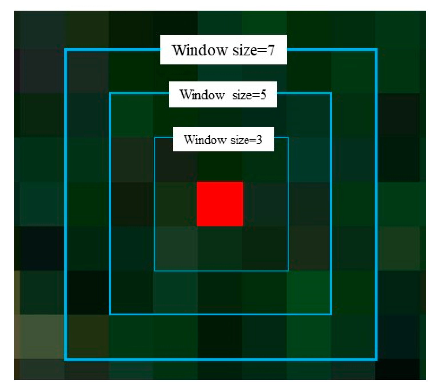
Remotesensing 12 00958 g001
Figure 2. An explanation of convolutional neural networks (CNN) inputs.
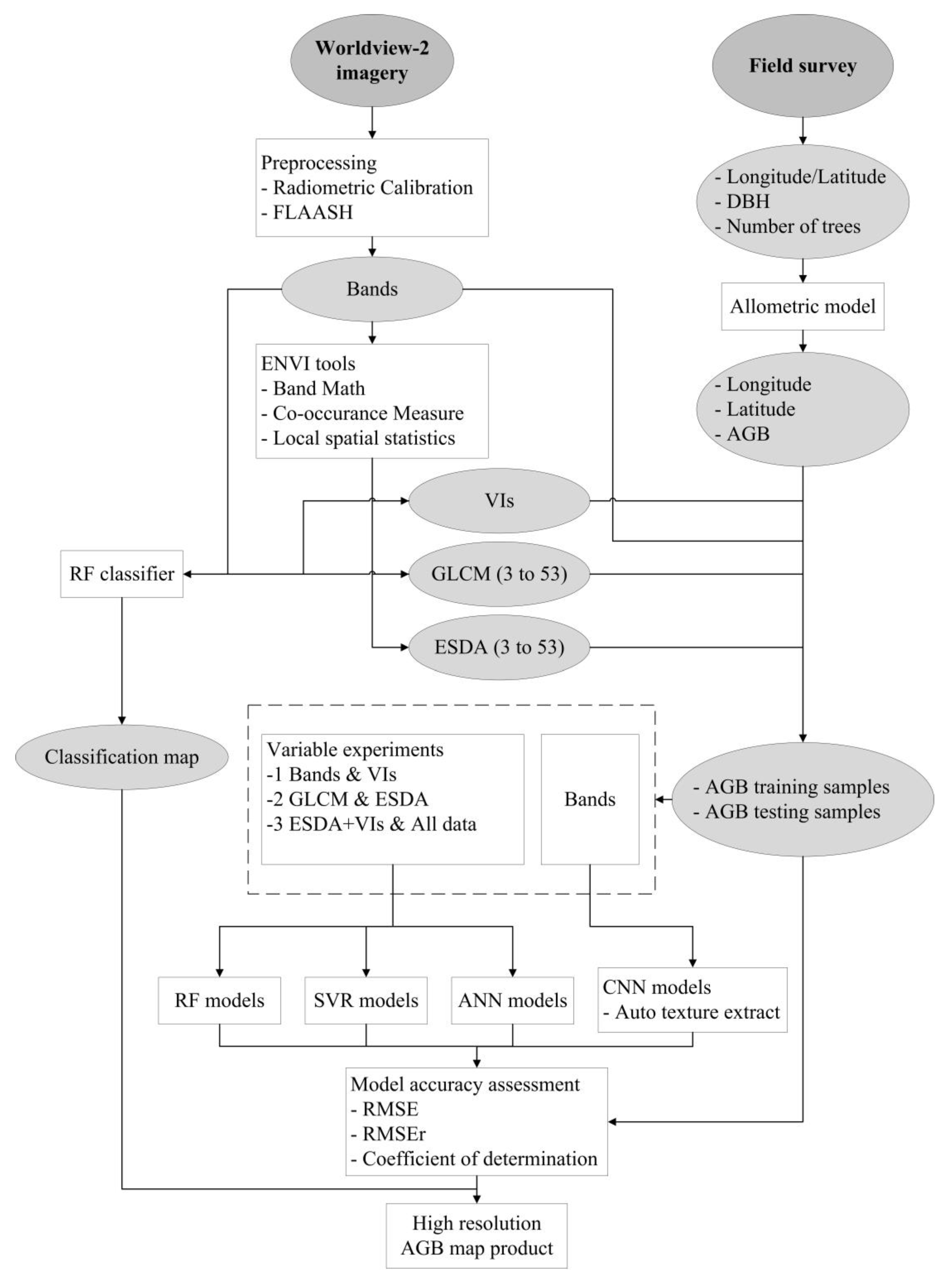
Remotesensing 12 00958 g002
Figure 3. Flowchart of steps used in our study for comparison of different algorithms and variables for above-ground biomass (AGB) estimation. The meanings of the abbreviations are listed as follows: The Environment for Visualizing Images (ENVI), the Fast Line-of-Sight Atmospheric Analysis of Spectral Hypercubes (FLAASH), Diameters at Breast Height (DBH), Random Forest (RF), Support Vector Regression (SVR), Artificial Neural Network (ANN), Root Mean Square Error (RMSE), Relative Root Mean Square Error (RMSEr).
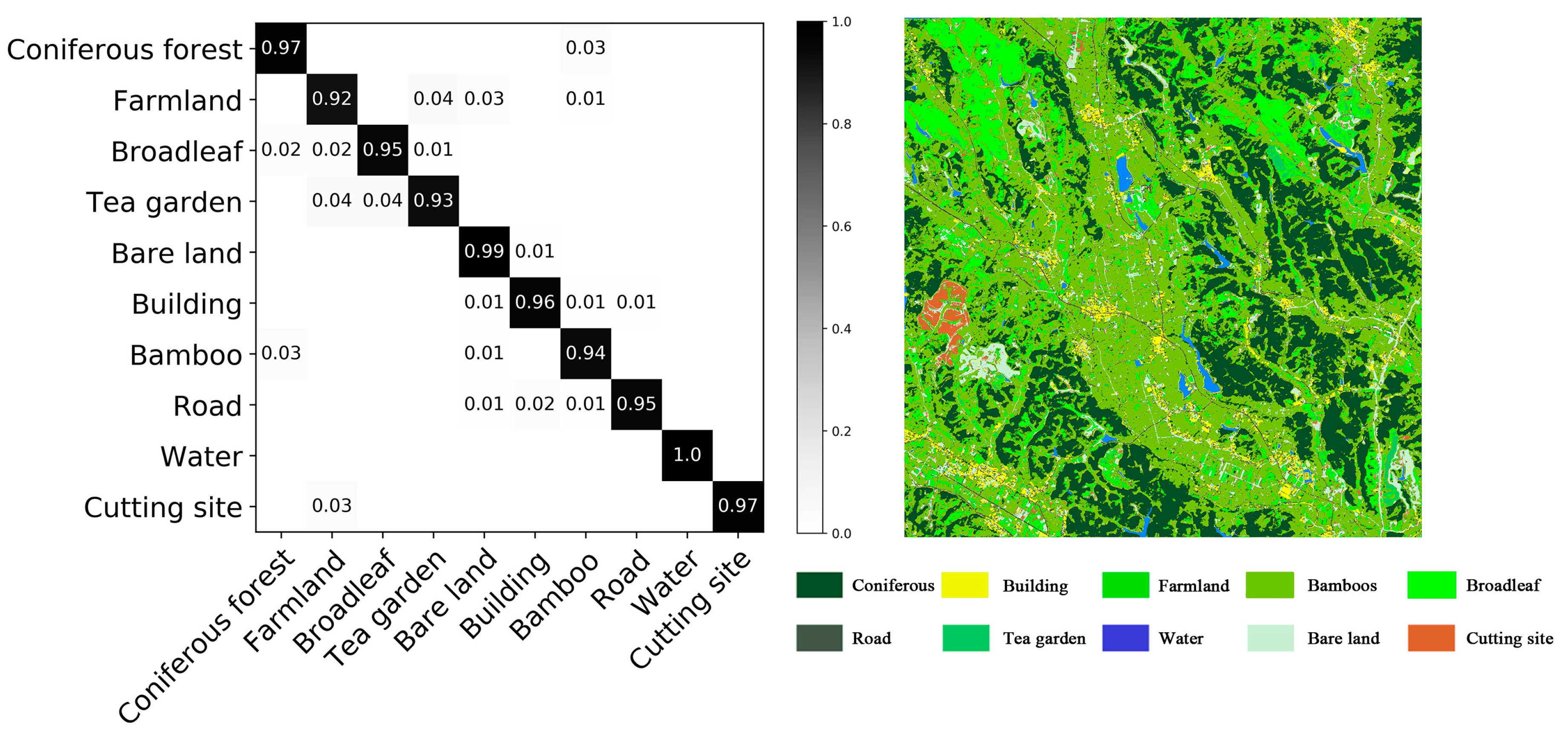
Remotesensing 12 00958 g003
Figure 4. Confusion matrix of classification results and classification map.
Remotesensing 12 00958 g004
Figure 5. The results of CNN with different window sizes. RMSE, RMSEr, and R square (R2) are used to evaluate the results. The average results of the 50 repeats are shown with triangles and the values are written right beside.
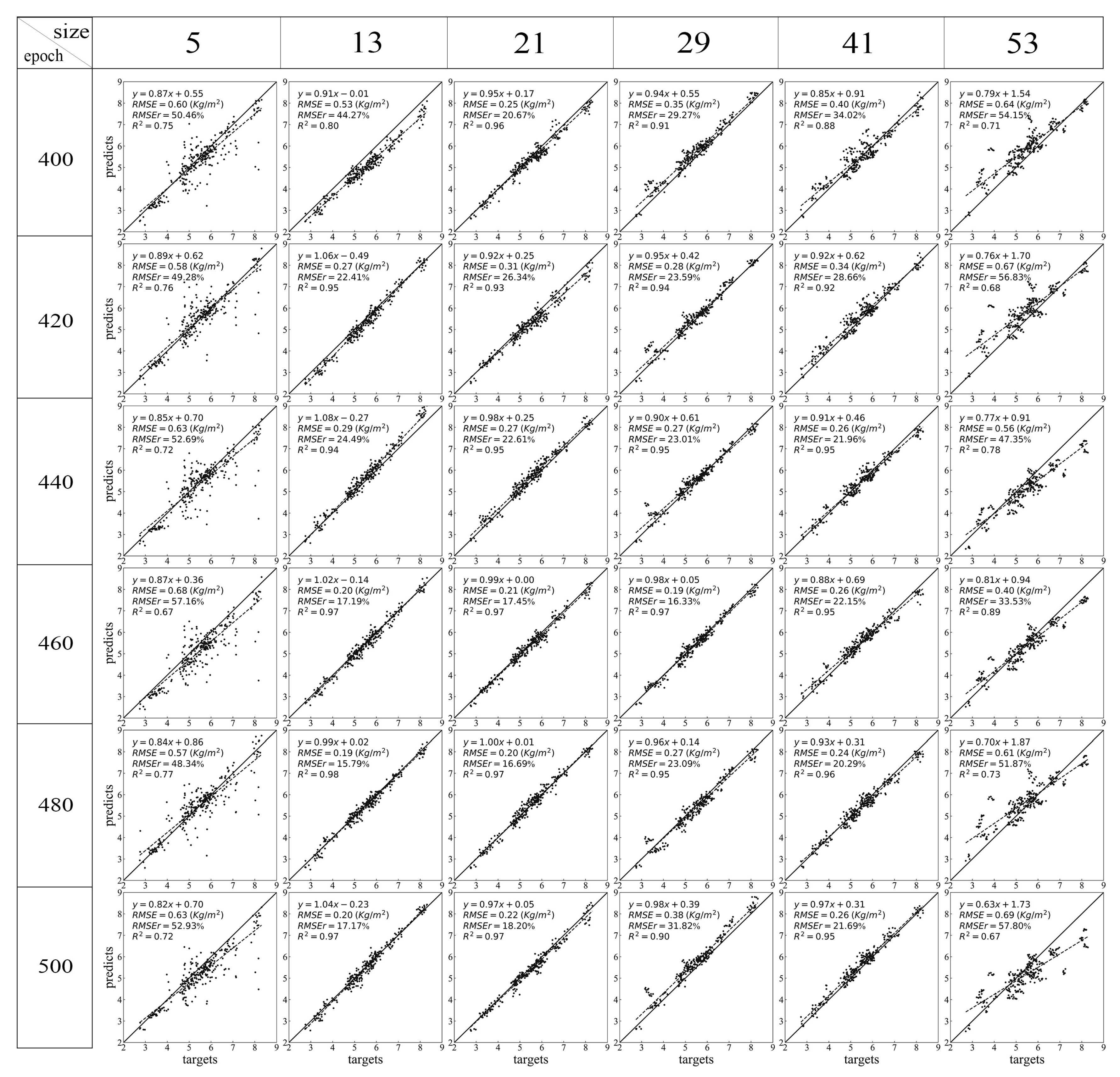
Remotesensing 12 00958 g005
Figure 6. Scatter plots of different epochs and window sizes of CNN. Different rows indicate the results from different training epochs and different columns indicate the results from inputs with different window sizes.
Remotesensing 12 00958 g006
Figure 7. The results (RMSE, RMSEr, R2) of bands and Vis + Bands using 3 Machine Learning (ML) algorithms with all the window sizes. (1) Figures of the left column are the results of three algorithms using bands. (2) Figures of the right column are the results of three algorithms using Vis + Bands.
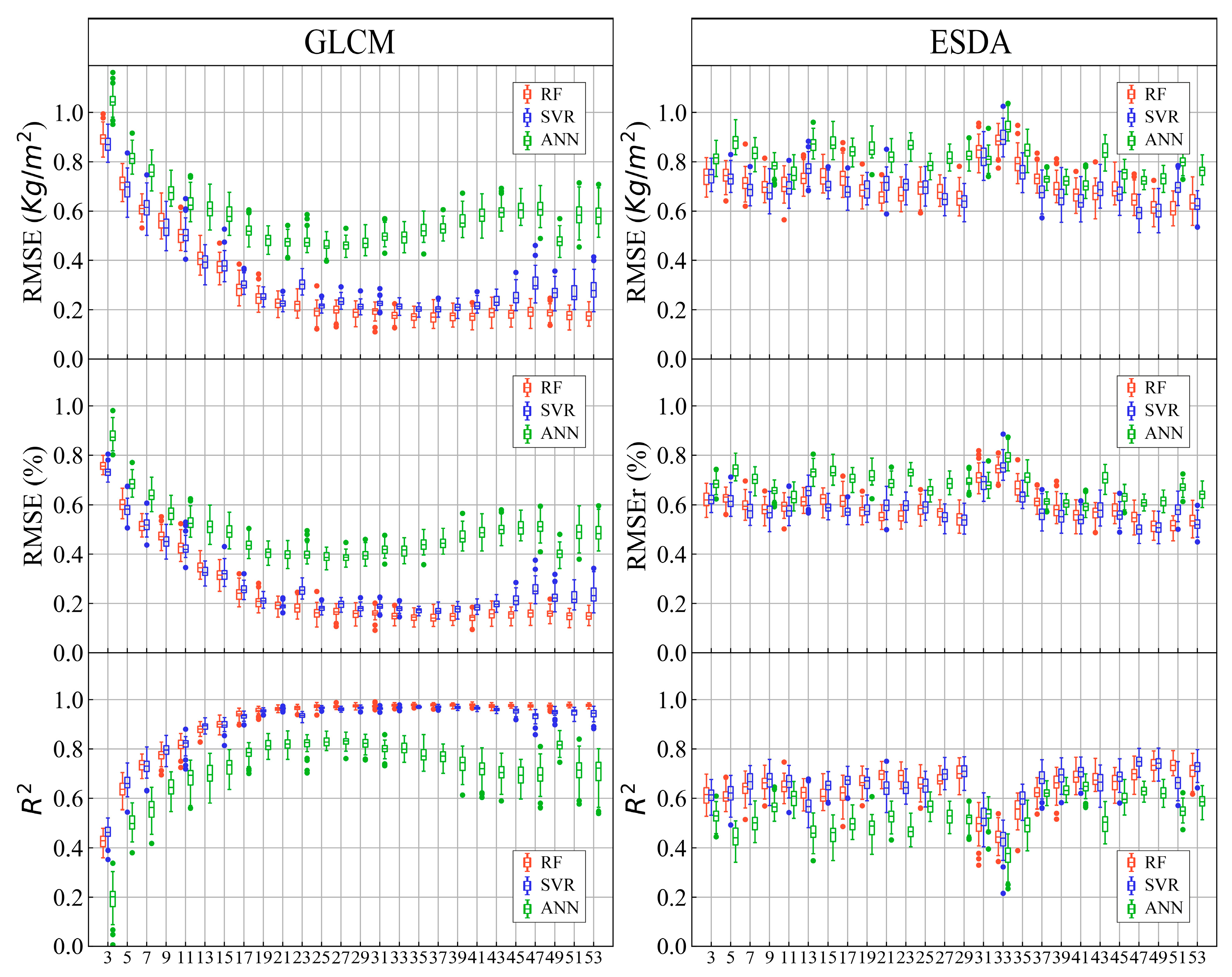
Remotesensing 12 00958 g007
Figure 8. The results (RMSE, RMSEr, R2) of GLCM + bands and ESDA + bands using 3 ML algorithms with all the window sizes. (1) Figures of the left column are the results of three algorithms using GLCM + band. (2) Figures of the right column are the results of three algorithms using ESDA + bands. Boxplots in red indicate RF; boxplots in blue indicate SVR; boxplots in green indicate ANN.
Remotesensing 12 00958 g008
Figure 9. The results (RMSE, RMSEr, R2) of all combined and ESDA + VIs using 3 ML algorithms with all the window sizes. (1) Figures of the left column are the results of three algorithms using All combined. (2) Figures of the right column are the results of three algorithms using ESDA + VIs. Boxplots in red indicate RF; boxplots in blue indicate SVR; boxplots in green indicate ANN.
Remotesensing 12 00958 g009
Figure 10. AGB maps using the 4 algorithms (RF, SVR, ANN, CNN). The mean values and standard deviation of 10 repeats were shown. RF algorithm used GLCM with a window size of 37, SVR of 35, and ANN with 27. CNN used bands as inputs and used a window size of 13.
Remotesensing 12 00958 g010
Figure 11. The mean value of 25 pixels of each plot. RF algorithm used GLCM with a window size of 37, SVR of 35, and ANN of 27. CNN used bands as inputs and used a window size of 13.
Remotesensing 12 00958 g011
Table 1. Formulas of the selected variables.
Feature TypesFeature NamesDetailsReferences
bandsGreen (G)450–510 nm\
Blue (B)510–581 nm
Red (R)630–690 nm
Near-infrared red (NIR)770–895 nm
Vegetation Indices (VIs)Difference Vegetation Index (DVI) N I R - R
Normalized Difference Vegetation Index (NDVI) ( NIR - R ) / ( NIR + R ) [57]
Normalized Difference Water Index (NDWI) ( G - NIR ) / ( G + NIR ) [58]
Ratio Vegetation Index (RVI) N I R / R
Exploratory spatial data analysis (ESDA)Moran’s I I i = z i j w i j z j c[50]
Geary’s C c i = j w i j ( z i z j ) 2 [50]
G statistic G i ( d ) = j w i j ( d ) z j z j [59]
Gray-level co-occurrence matrices (GLCM)Mean (MEA) M E A = i ,   j = 0   N 1 i P i , j [54]
Variance (VAR) V A R = i ,   j = 0   N 1 P i , j ( 1 μ i )
Homogeneity (HOM) H O M = i ,   j = 0   N 1 i P i , j 1 + ( i j ) 2
Contrast (CON) C O N = i ,   j = 0   N 1 i P i , j ( i j )
Dissimilarity (DIS) D I S = i ,   j = 0   N 1 i P i , j | i j |
Entropy (ENT) E N T = i ,   j = 0   N 1 P i , j l n P i , j
Augular Second Moment (ASM) A S M = i ,   j = 0   N 1 i P i , j 2
Correlation (COR) C O R = i ,   j = 0   N 1 i i , j   N 1 i j P i , j μ i μ i σ i 2 σ j 2
Note: μ i = i = 0 N 1 i j = 0 N 1 P i , j
σ i = j = 0 N 1 ( i μ i ) 2 j = 0 N 1 P i , j
Table 2. Basic statistics of the field measured plant density, average DBH (D), and above ground biomass (AGB). Maximum value (Max), Minimum value (Min), mean value (Mean), Standard Deviation (SD) and Coefficient of Variation (CV) are listed.
Density (Plant/m2)D (cm)AGB (kg/m2)
Max5.1604.6718.175
Min1.8402.9432.815
Mean3.3473.9135.451
SD0.7550.3721.200
CV22.5%9.5%22%
Table 3. Classification results using GLCM and bands. The meanings of columns are as follows: CF: coniferous forest, FA: farmland, BR: broadleaf forest, TE: tea garden, BL: bare land, BU: building, BB: bamboo, RO: road, WA: water, CS: cutting site.
CFFABRTEBLBUBBROWACS
User Accuracy (UA)0.970 0.918 0.952 0.927 0.988 0.965 0.941 0.955 1.000 0.966
Producer Accuracy (PA)0.946 0.882 0.962 0.950 0.934 0.953 0.960 0.988 1.000 1.000
Overall Accuracy (OA)0.957
Kappa coefficient (kappa)0.952
Table 4. Parameter settings of random forest (RF) and support vector regression (SVR). For RF, the values of mtry and ntree for all the feature set are listed. For SVR, the values of C (cost of misclassification) and ε (the influence of a single sample).
FeatureRFSVRANN
mtryntreeDenotationCεDenotationDenotation
bands22000Bands_RF10000.1Bands_SVRBands_ANN
VIs32000VIs_RF100.1VIs_SVRVIs_ANN
GLCM412000GLCM_RF_x0.80.01GLCM_SVR_xGLCM_ANN_x
ESDA52000ESDA_RF_x150.01ESDA_SVR_xESDA_ANN_x
ESDA+VIs62000ESDA+VIs_RF_x0.80.1ESDA+VIs_SVR_xESDA+VIs_ANN_x
All combined482000All_RF_x0.80.1All_SVR_xAll_ANN_x
x is a number to indicate the window size of the texture variables.
Table 5. The results (RMSE, RMSEr, R2) of bands and Vis + bands using 3 different algorithms. In this table, the mean values of 50 repeats are calculated. The highest result of each scenario is denoted in bold.
AlgorithmsBandsBands+VIs
RMSE (Kg/m2)RMSErR2RMSE (Kg/m2)RMSErR2
RF1.1470.9610.0761.1580.9750.049
SVR1.1710.9740.0461.1600.9730.052
ANN1.0410.8720.2381.0320.8670.248
Table 6. The results (RMSE, RMSEr, R2) of GLCM + bands and ESDA + bands using 3 different algorithms. In this table, the mean values of 50 repeats were calculated. Then the best result of all window sizes is reported as well as the window size. The highest result of each scenario is denoted in bold.
AlgorithmsGLCMESDA
RMSE (Kg/m2)RMSErR2Window SizeRMSE (Kg/m2)RMSErR2Window Size
RF0.1690.1420.979370.6100.5140.73551
SVR0.2030.1700.970350.7490.5000.59147
ANN0.4600.3870.831270.7080.5940.64641
Table 7. The results (RMSE, RMSEr, R2) of all combined and ESDA + VIs using 3 different algorithms. In this table, the mean values of 50 repeats are calculated. Then the best result of all window sizes is reported as well as the window size. The highest result of each scenario is denoted in bold.
AlgorithmsAll CombinedESDA + VIs
RMSE (Kg/m2)RMSErR2Window SizeRMSE (Kg/m2)RMSErR2Window Size
RF0.1930.1620.974510.6410.5360.71249
SVR0.2110.1780.968350.6270.5280.72147
ANN0.4300.3610.855310.5740.4820.76541

