Design of Feedforward Neural Networks in the Classification of Hyperspectral Imagery Using Superstructural Optimization

Abstract

Artificial Neural Networks (ANNs) have been used in a wide range of applications for complex datasets with their flexible mathematical architecture. The flexibility is favored by the introduction of a higher number of connections and variables, in general. However, over-parameterization of the ANN equations and the existence of redundant input variables usually result in poor test performance. This paper proposes a superstructure-based mixed-integer nonlinear programming method for optimal structural design including neuron number selection, pruning, and input selection for multilayer perceptron (MLP) ANNs. In addition, this method uses statistical measures such as the parameter covariance matrix in order to increase the test performance while permitting reduced training performance. The suggested approach was implemented on two public hyperspectral datasets (with 10% and 50% sampling ratios), namely Indian Pines and Pavia University, for the classification problem. The test results revealed promising performances compared to the standard fully connected neural networks in terms of the estimated overall and individual class accuracies. With the application of the proposed superstructural optimization, fully connected networks were pruned by over 60% in terms of the total number of connections, resulting in an increase of 4% for the 10% sampling ratio and a 1% decrease for the 50% sampling ratio. Moreover, over 20% of the spectral bands in the Indian Pines data and 30% in the Pavia University data were found statistically insignificant, and they were thus removed from the MLP networks. As a result, the proposed method was found effective in optimizing the architectural design with high generalization capabilities, particularly for fewer numbers of samples. The analysis of the eliminated spectral bands revealed that the proposed algorithm mostly removed the bands adjacent to the pre-eliminated noisy bands and highly correlated bands carrying similar information.

1. Introduction

Since the introduction of perceptron by Rosenblatt in 1958 [1], numerous studies in almost all scientific fields have been conducted to apply neural network models and test their performances. Starting with the first pioneering study of Benediktsson et al. [2], artificial neural networks (ANNs) have been extensively used in remote sensing fields, frequently for the supervised classification of remotely sensed images in the production of thematic maps [3,4,5,6]. Historical development reveals that ANNs were initially applied for comparative studies with conventional classifiers (e.g., maximum likelihood classifier), and later with other machine learning algorithms (e.g., support vector machines, random forest) for a wide range of problems [7,8,9,10,11]. In the last decade, new and advanced satellite sensors were launched, producing a vast amount of data repeatedly, at a higher number of bands. Both spatial and spectral resolutions of the sensors have increased; thus, the selection of the most appropriate data as inputs, known as feature selection, has become a more critical issue, particularly for neural networks. For this purpose, the pruning of neural networks has been suggested as an alternative to existing statistical methods [12,13,14,15].

The topology of Multi-Layer Perceptron (MLP) networks includes three types of layers called input, hidden, and output layers, each consisting of fully interconnected processing nodes, except that there are no interconnections between the nodes within the same layer. These networks typically have one input layer, one or more hidden layers, and one output layer. The input layer nodes correspond to individual data sources, which can be either spectral bands or other sources of data. The output nodes correspond to the desired classes of information, such as land use/land cover (LULC) classes in classification. Hidden layers are required for computational purposes. The values at each node are estimated through the summation of the multiplications between previous node values and weights of the links connected to that node. Since the nodes on input and output layers are usually pre-defined, except for the feature selection case where some irrelevant or highly correlated inputs are eliminated, the number of hidden layers and their nodes are the unknown hyper-parameters in the network, the choice of which directly affects the performance and generalization capabilities of the network. Several heuristics and formulations have been suggested in literature to estimate the optimal size for the hidden layer(s), but there is no universally accepted method that exists for estimating the optimal number of hidden layer nodes for a particular problem [16,17,18,19]. The use of ANNs in remote sensing has been reviewed by several studies, including [17,19,20,21]. Furthermore, the limitations and crucial issues in the application of neural networks have been discussed in [17,19,21,22].

Several approaches or methods exist in literature for the construction of optimal network architecture in addition to the heuristics mentioned above. These methods can be categorized as exhaustive search algorithms, also known as brute-force, constructive, pruning, and a combination of these methods. In the brute-force approach, after many small network architectures are formed and trained, the best smallest architecture producing the lowest error level or the highest accuracy for the dataset is selected. This approach is computationally expensive since many networks must be trained to obtain a solution [22,23]. Constructive methods start with a small network and add new hidden nodes to the network after each epoch if the training error or the proposed accuracy is not at the acceptable level. On the other hand, pruning methods work opposite to the constructive methods, in that a large network is selected and unimportant or ineffective links and/or hidden layer nodes are removed. Thus, overfitting to the training data can be avoided. These methods have the advantages of both small and large networks. For a start, the user has to determine the initial large network structure for the problem and the stopping criterion to end the training process. It was reported that training a large network and then pruning it is advantageous and favorable compared to that of training a small network [17,24]. There are also hybrid methods, also known as growing and pruning methods, that can both add and remove hidden layer units [25,26,27,28]. These methods are less popular due to the training of small networks suffering from the noisy fitness evaluation problem, and they are likely to be stuck into a local minimum together with a longer training time requirement.

The design of a neural network is not a simple task. The number of nodes in the hidden layer(s) should be large enough for the correct representation of the problem, but at the same time low enough to have adequate generalization capabilities [29]. The optimum number of hidden layer nodes depends on various factors including the numbers of input and output units, the number of training cases, the complexity of the classification to be learned, the level of noise in the data, the network architecture, the nature of the hidden unit activation function, the training algorithm, and regularization [30]. It is impractical to state that neural network topology is minimal and optimal since the optimality criteria actually varies for each problem under consideration [31]. If the network is too small, it cannot learn from the data, resulting in a high training error, which is a characteristic of underfitting. Small networks can have better generalization capabilities, but there is a risk of not learning the problem under consideration due to the insufficient number of processing elements [23,32]. On the other hand, if the network is too large, a well-known overfitting problem occurs. In other words, it becomes over-specific to the training data and likely to fail with the test data, producing lower classification accuracies. However, large networks have better fault tolerance [33]. Ideally, a close correspondence between training and testing errors is desired [34]. From the above argument, it can be concluded that a large network should be preferred to a small one since underfitting is a more serious issue than overfitting as it can be avoided using training strategies and pruning techniques by downsizing the network wisely. The optimum structure for a neural network should be large enough to learn the underlying characteristics of the problem and small enough to generalize for other datasets [17,32]. The motivation in this study is to not only remove some interconnections or eliminate some hidden layer neurons to improve generalization capabilities, but also to reduce the dimension of the input layer by eliminating the least effective and correlated spectral bands, and thus achieve improved performance. This is particularly important for the processing of hyperspectral images that comprise many correlated and sometimes irrelevant spectral bands for the problem under consideration.

Sildir and Aydin [35] suggested using a mixed-integer programming method in order to optimally and simultaneously design and train ANNs via superstructure optimization and parameter identifiability. In this study, a similar superstructure-based optimization technique is proposed for the classification of two benchmark hyperspectral images. The first essential part of the suggested method is to set up the superstructure formulation where inputs, number of neurons, and connections between inputs, hidden neurons, and outputs are all binary decision variables. At the same time, standard ANN parameters, e.g., connection weights, can take continuous values. This strong formulation brings about a mixed-integer program, usually, a nonlinear one (MINLP), which has to be solved with respect to a certain design metric. As a result, ‘redundant’ input variables, neurons, and connections for larger datasets are eliminated automatically.

In addition to the superstructure formulation, we also suggest integrating the use of statistical measures, namely parameter uncertainty for the purpose of enhancing the prediction performance of ANNs. This statistical approach takes the covariance of ANN parameters into account and integrates the measure with the objective function of the training algorithm. To the best of authors’ knowledge, this paper is the first application of such an optimal and robust ANN algorithm addressing the classification of remotely sensed imagery. In addition to this novel application concept, extra linking constraints are added to this newer formulation that forces the optimization algorithm not to iterate for the continuous variables when certain binary variables are equal to zero, which in turn decreases the computational load of the resulting mixed-integer type ANN related problems significantly.

2. Test Sites and Datasets

For the experiments, aimed to show the effectiveness of the proposed optimization algorithm, two well-known hyperspectral datasets that are widely used in literature to test new algorithms and approaches were employed in this study. The effectiveness of the proposed method was investigated with different sampling ratios using 10% and 50% of the ground reference data.

2.1. The Indian Pines Dataset

The Indian Pines scene recorded by the Airborne Visible/Infrared Imaging Spectrometer (AVIRIS) sensor on June 12, 1992, was used in this study. The image and its ground reference data are made available by Purdue University (https://purr.purdue.edu/publications/1947/1). The dataset, covering a 2.9 by 2.9 km (145 by 145 pixels) agriculture dominated land in Tippecanoe County of Indiana, USA, has 220 spectral bands at 20 m spatial resolution (Figure 1). Twenty spectral bands (104–108, 150–163, 220) comprising the region of water absorption were removed from the dataset. The ground reference dataset including 16 LULC classes was collected through a field study in June 1992 [36]. The Indian Pines dataset has been employed in many publications to test and compare the performances of various algorithms [37,38]. The dataset is regarded as a challenging one for classification problems because of three major reasons. Firstly, the crops in the study site (mainly corn and soybeans) were very early in their growth cycle (about 5% canopy cover). Secondly, the imagery has a moderate spatial resolution of 20 m, resulting in a high number of mixed pixels. Lastly, the number of reference samples for the 16 LULC classes varies greatly among the classes, ranging from 20 samples to 2,455, which is regarded as an imbalanced dataset. Because of the availability of the limited number of samples for each LULC class, many researchers either combined the particular class types into a single one or avoid using some of the classes (e.g., oats, alfalfa, stone-steel towers). Considering that 20 pixels of the oats class must be divided into training and testing in the application that makes the learning process theoretically challenging, this class is left out in further processes. Thus, the Indian Pines dataset with 15 LULC classes, which are shown in

Table 1. Descriptions of the classes for Indian Pines data.

Index	Description	Number of Samples
O1	Alfalfa	54
O2	Corn-notill	1,434
O3	Corn-min	834
O4	Corn	234
O5	Grass-pasture	497
O6	Grass-trees	747
O7	Grass-pasture-mowed	26
O8	Hay-windrowed	489
O9	Soybean-notill	968
O10	Soybean-min	2468
O11	Soybean-clean	614
O12	Wheat	212
O13	Woods	1294
O14	Buildings-Grass-Trees-Drives	380
O15	Stone-Steel towers	95

, was considered in this study.

2.2. The Pavia University Dataset

The Pavia University hyperspectral image was acquired with a Reflective Optics Spectrographic Image System (ROSIS) sensor during a flight campaign over Pavia, northern Italy. The ROSIS optical sensor provides images at a spectral range from 0.43 to 0.86μm with 115 bands. Twelve bands that were noisy or impacted by water absorption were removed from the dataset and the remaining 103 bands were employed in this study. The dataset captured over the Engineering School of the Pavia University has 610 × 340 pixels with a spatial resolution of 1.3 m. The Pavia University dataset has ground truth maps of 9 classes and 42,776 labeled samples. The image and the ground reference data are shown in Figure 2 and details about the samples of all classes are given in

Table 2. Descriptions of the classes for Pavia University data.

Index	Description	Number of Samples
O1	Asphalt	6631
O2	Meadows	18,649
O3	Gravel	2099
O4	Trees	3064
O5	Painted metal sheets	1345
O6	Bare soil	5029
O7	Bitumen	1330
O8	Self-blocking bricks	3682
O9	Shadows	947

.

3. Optimal ANN Structure Detection and Training Methodology

Typical ANN structures usually contain a single hidden layer in addition to input and output layers containing identity activation functions. All those layers are fully connected in a traditional sense. The expression for a typical fully connected ANN (FC-ANN) is given by:

$$y=f_1\left(A\cdot f_2\left(B\cdot u+C\right)+D\right)$$

(1)

where A, B, C, and D are continuous weights with proper dimensions; f₁ and f₂ are output and hidden layer activation functions, respectively. For classification problems, the selected output activation function usually used for normalization. The softmax function is a typical example among other alternatives [39]. Note that the output activation function also calculates the individual probabilities for the classification problems, whereas the hidden layer activation function is not necessarily limited to normalization.

For an FC-ANN, the weights are traditionally assigned as non-zero in order to represent the connections among the neural network variables and layers. Those weights are estimated in the training by nonlinear optimization through the solution of:

$$Mi{n}_{A,B,C,D}{\displaystyle \sum }_{i=1}^N\Vert f_1\left(A\cdot f_2\left(B\cdot u_i+C\right)+D\right)-y_i\Vert$$

(2)

where N is the number of training samples; $y_i$ is the i^th sample vector; $u_i$ is the i^th input vector. Note that Equation (2) might also include additional box constraints to either reduce the search space for the training of ANNs or for specifically tailoring the training formulation.

As mentioned above, the solution of Equation (2) is usually obtained via programming a non-linear optimization problem (NLP). This solution delivers the FC-ANN weights (continuous variables), which minimize the training error without considering parameter identifiability issues, architecture orientation, and overfitting. In theory, as the number of decision variables and connections increases, the ANN training formulation should generate more flexibility, which in turn enhances the representative nature of ANNs on more complex datasets. The numbers of outputs, inputs, and hidden layer neurons together represent the number of decision variables. Traditionally, the structural hyper-parameters including the number of neurons, contained layers with the neurons, and the activation functions are manually tuned after trial and error. In addition to the structural parameters, the selection of proper input variables is another vital decision that is not included in (2) explicitly. However, it should be noted that complex and large datasets contain a significant amount of correlation and redundancy, especially in the big data era. On the other hand, it should be mentioned that deep neural networks including dropout layers can easily deal with the overfitting issues in a sequential manner. Yet, using deep neural nets is not in the scope of this paper. The integration of the proposed novel structure detection and training algorithm with the deep neural networks, which can be carried out without a loss of generality, is left for a future study.

Once the number of neurons lifts up, the dimension of continuous variables increases proportionally, and more connections are introduced in FC-ANNs. As a result, FC-ANN architecture becomes more challenging to train. Moreover, the optimal estimation of those parameters suffers from identifiability issues when the ANN architecture is poorly designed, or the training data do not contain statistically significant information [40,41,42,43].

The covariance matrix of the continuous ANN parameters have been adopted as a measure of identifiability in previous studies ([44]) and is used as a statistical metric in this study, for the elimination of the ANN variables including the number of neurons, connections, and input variables. Once the sum of the elements of the covariance matrix has a higher numerical value, the accompanying uncertainty in that estimated parameter leads to much larger prediction bounds due to the prorogation of uncertainty ([45]). In addition, a significant amount of computational power might be required for the training of ANNs, since there are many combinations of parameter values resulting in similar training performances.

Sildir and Aydin ([35]) proposed an MINLP formulation that realizes the optimal training of ANNs via superstructure modifications and parameter identifiability. They showed the contribution of the proposed formulation on regression problems. Results showed that the suggested method increases the predictive capabilities of ANNs with a significant reduction in the ANN superstructure compared to FC-ANNs. The MINLP formulation introduces additional binary variables to the traditional ANN equations in order to detect the optimal ANN architecture and to favor the optimal determination of input variables, hidden neurons, and connections for larger datasets among a maximum ANN structure. The modified one hidden layer ANN output equation is given as follows:

$$y=f_1\left(\left(A\circ A_{binary}\right)\cdot diag\left(N_{binary}\right)\cdot f_2\left(\left(B\circ B_{binary}\right)\cdot diag\left(U_{binary}\right)\cdot u+C\right)+D\right)$$

(3)

where $\circ$ is the Hadamard product operator; $A_{binary}$ and $B_{binary}$ are matrices with binary values representing the existence of connections. The existence of a particular connection is defined by the binary variable $A_{binary,ij}$. A_ij is the continuous weight parameter of the connection between the j^th neuron and the i^th output and can be non-zero only if the connection is decided to exist after solving the training optimization problem. Similarly, B_ij represents the connection between the input and corresponding neurons. In practice, once a particular column of B_ij is zero, then the j^th input does not deliver information to the hidden layer and thus to the outputs as a result of feed-forward design. $N_{binary}$ and $U_{binary}$ are the binary vectors defining the existence of the neuron and input, respectively. For instance, if a particular element of $U_{binary}$ is zero, it makes the corresponding column of $B_{binary}$ zero, eliminating all the connections from the particular input; thus, the corresponding input is eliminated. These rules are realized via the introduction of extra linking constraints to the formulation, and the resulting problem exhibits a strong mixed-integer program formulation. The training optimization problem is given by:

$$\begin{array}{c}Mi{n}_{A,A_{binary},B,B_{binary},C,D,N_{binary},U_{binary}}\gamma \sum diag\left(co{v}_p\right)+F\\ s.t.\\ F={\displaystyle {\displaystyle \sum }_{i=1}^N}\Vert f_1\left(\left(A\circ A_{binary}\right)\cdot diag\left(N_{binary}\right)\cdot f_2\left(\left(B\circ B_{binary}\right)\cdot diag\left(U_{binary}\right)\cdot u_i+C\right)+D\right)-y_i\Vert \\ A_{binary,ij}\le N_{binary,j}\\ B_{binary,ij}\le U_{binary,j}\\ -A_{LB}\times A_{binary,j}\le A_{i,j}\le A_{UB}\times A_{binary,j}\\ -B_{LB}\times B_{binary,j}\le B_{i,j}\le B_{UB}\times B_{binary,j}\\ A_{binary},B_{binary},N_{binary},U_{binary}\in \left\{0,1\right\}\end{array}$$

(4)

where γ is the tuning parameter for the multi-objective optimization; $A_{LB}$ and $A_{UB}$ are lower and upper bounds on A respectively; $B_{LB}$ and $B_{UB}$ are lower and upper bounds on B respectively ([35]). $co{v}_p$, which is a measure of parameter identifiability in this formulation, is the covariance matrix of the estimated ANN weights. Intuitively, diagonal elements of this refer to the variances of the corresponding weight. In theory, those values would increase significantly when overfitting occurs.

The problem given in Equation (4) is a relatively large scale and non-convex MINLP, which is quite challenging to solve to the global optimum. There are various efficient commercial solvers utilizing branch and bound ([46]), generalized benders decomposition ([47]), and outer approximation methods ([48]) for solving convex MINLPs. Nevertheless, solving non-convex MINLPs to global optimality is still an open research area and is not in the scope of this study. We should also mention that both the training and testing performances of the ANNs can be increased dramatically when a global solution algorithm is implemented to solve the problem given in Equation (4).

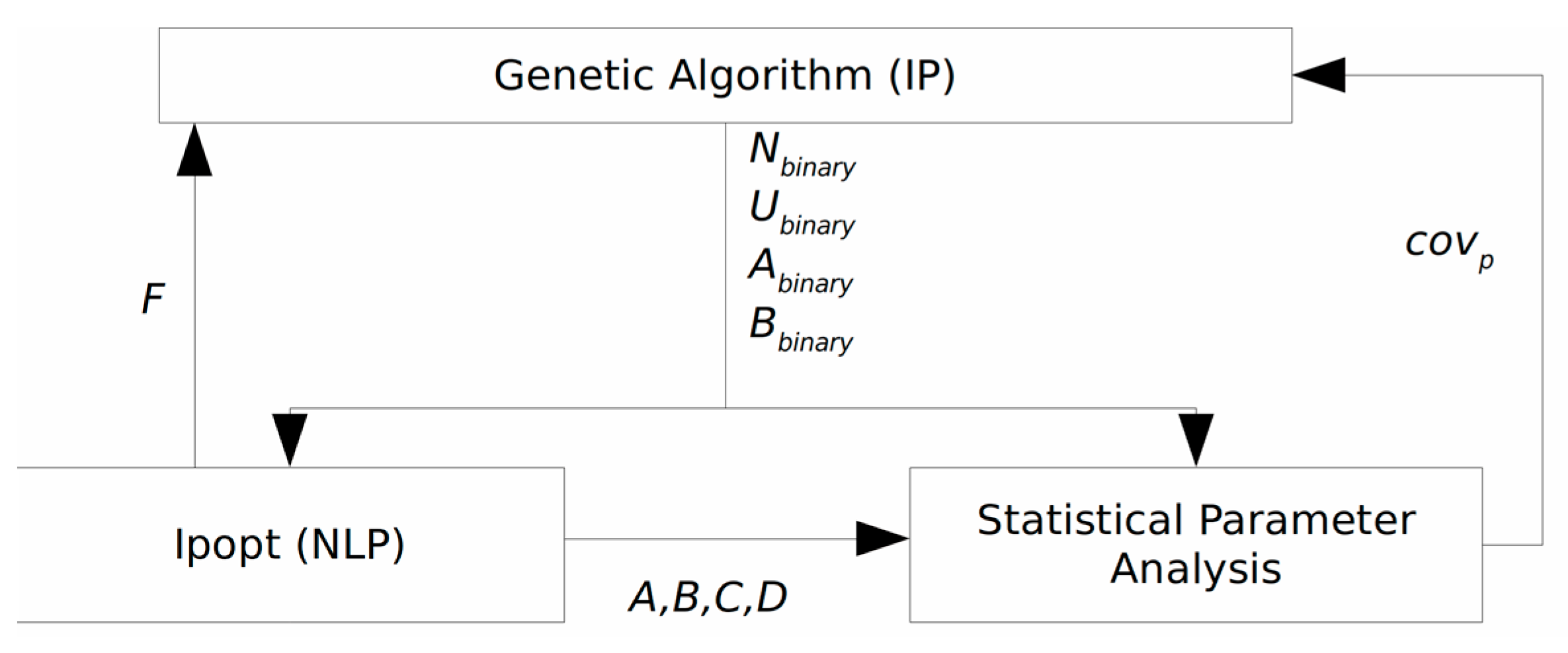
In this work, the adaptive, hybrid evolutionary algorithm suggested in [35] is used to solve the non-convex MINLP program given by (4). This method decomposes the original MINLP into integer programming (IP) and nonlinear programming (NLP) problems ([49,50,51]). IPs only include integer (or binary) decision variables that can be adjusted during optimization, whereas NLPs only involve continuous decision variables. For detailed information about the aforementioned optimization problems and their solution methods, we refer the reader to [52]. The IP stands on the outer loop and is solved via the genetic algorithm-based IP solver of Matlab while the inner loop NLP is solved by an interior point-based open source nonlinear programming solver IPOPT ([53]). Two problems are solved sequentially until the tolerance value of the original problem objective value or the maximum wall clock time is reached. This quasi decomposition feature is usually beneficial for solving large-scale problems. It should be noted that all the experiments in this study were carried out using our in-house programs in Matlab software (v.2019b). The fully connected network (FC) was trained using the Matlab Neural Net Toolbox, implementing a standard back-propagation algorithm for training. A pseudo-algorithm for the mentioned optimal ANN structure detection and training approach is shown in

Table 3. Pseudo algorithm adopted in this study for superstructure optimization.

Begin Start with an initial guess and calculate the objective function While (t<Maximum Wall Cock Time) or (Stopping Criterion)  Assign binary decision variables  Update linking constraints  While (Iteration number < Criterion) or (Stopping Criterion)   Update continuous decision variables  End While  Calculate the covariance matrix of parameters  Calculate the objective function  If (Objective function is improved)   Update binary decision variables (e.g., the ANN structure)  End If End While

. Also, a simplified diagram of the problem solution is shown in Figure 3.

There are efficient duality-based decomposition algorithms, which have proven to be very powerful for solving non-convex MINLP problems to global optimality. Nevertheless, these methods often require the NLP to be solved to global optimality, which is a challenging task for highly nonlinear relations (e.g., the tanh function of ANNs), and they demand high computational power. Unless the NLP converges to global optima, the decomposition algorithm may converge to an infeasible point or even diverge. On the other hand, these requirements do not usually apply to adaptive black-box optimization methods, with the possible drawback of converging to local optima. As mentioned above, the solution of the suggested ANN training problem to global optimality is not in the scope of this work and is left to a future study.

4. Results

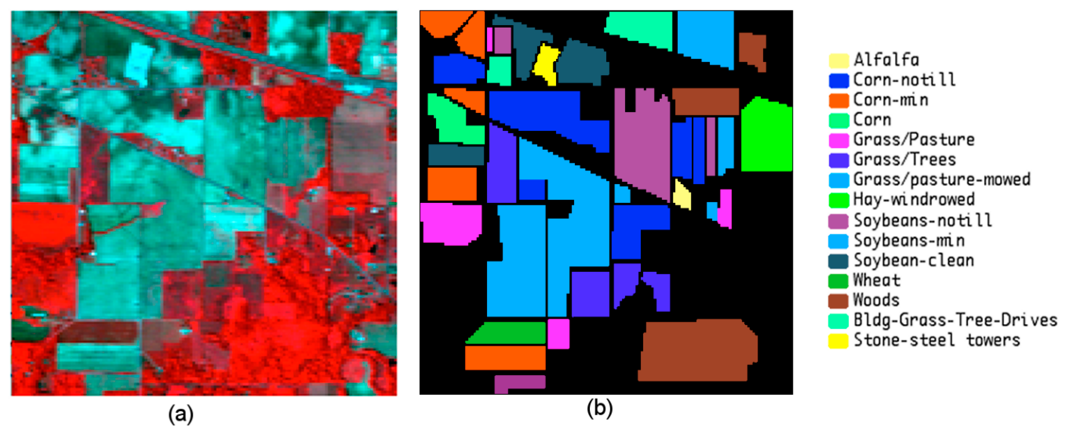
The optimization problem given in Equation (4) was solved for the two public datasets considered in this study. The ANN architecture obtained from Equation (4) is called the optimal superstructure ANN (designated as OS hereafter) whose performance is compared to the fully connected ANN (designated as FC hereafter) to show the contribution of the current approach. Unlike FC, OS contains a significantly smaller number of neurons and connections, produced by eliminating the least effective or redundant hidden neurons, interconnections, and input variables. In order to test the effect of sample sizes used in the training process, 10% and 50% samples of the whole dataset were employed in the processing of FC and OS neural networks. For the Indian Pines dataset, 1082 training samples for the 10% sampling ratio and 5,173 training samples for the 50% sampling ratio using 200 spectral bands as inputs were considered for the prediction of 15 LULC classes.

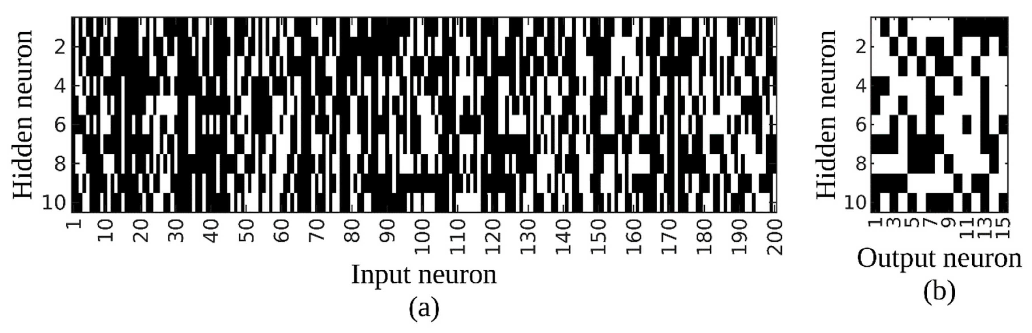
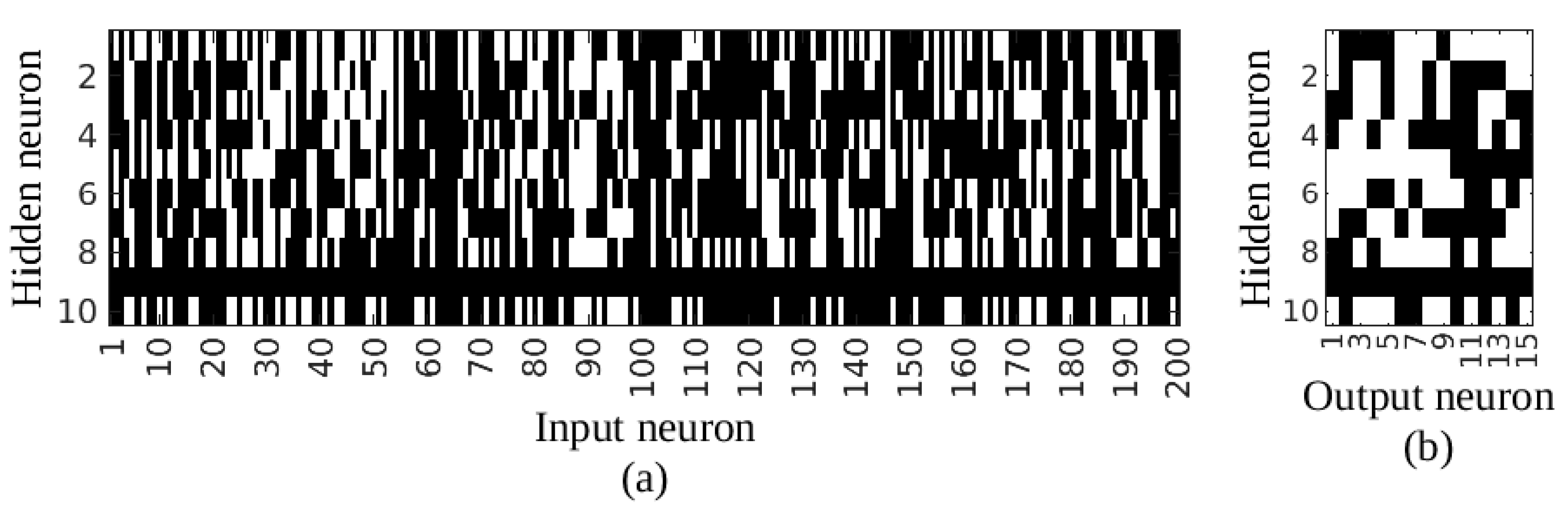
Figure 4 represents the remaining connections within the network with the white color representing a non-zero value, and thus existing connections, and the black color showing the removed connections for the network trained with approximately 10% sampling ratio. Whilst Figure 4a shows the connections between input and hidden layers, Figure 4b shows the connections between hidden and output layers. It can be noticed easily that no hidden layer node was removed from the network; thus, only the connections were removed by the proposed method. The final structure of the network was estimated as 158-10-15, indicating that 42 inputs (i.e., spectral bands) that have no connection to any hidden neuron were eliminated, represented by a black column in Figure 4a. On the other hand, 1,271 of 2,150 connections, representing 61% of the total connections, were also removed from the network to simplify the network and improve its generalization capabilities.

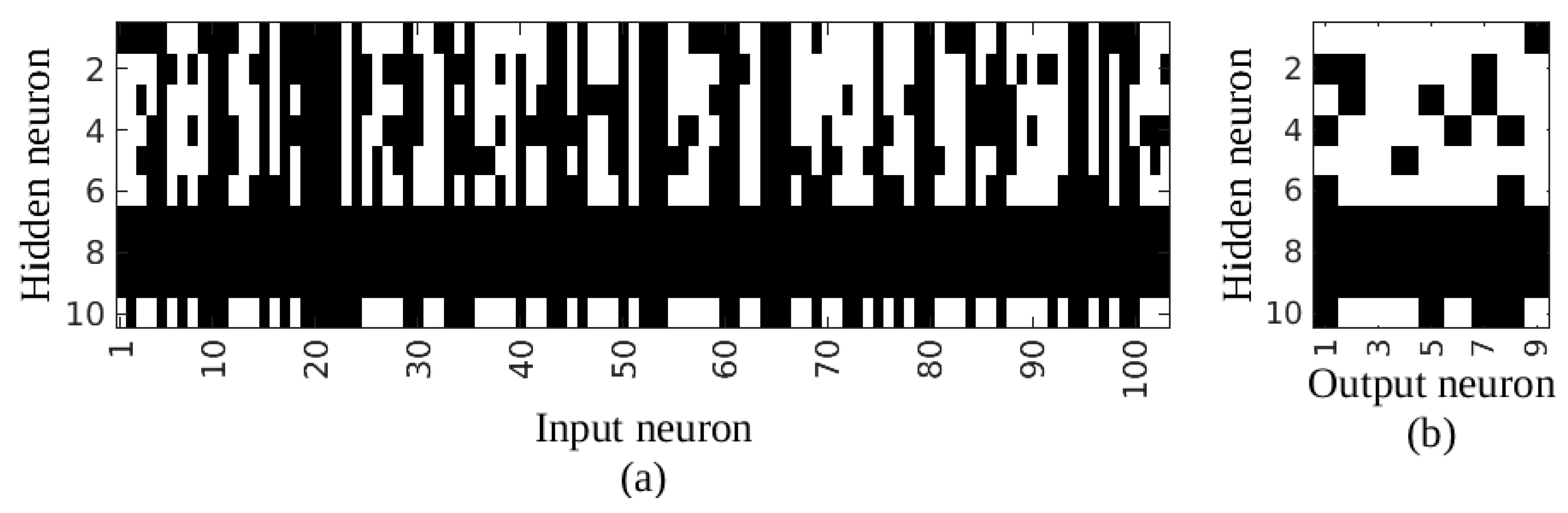
For the 50% sampling ratio, an optimal network superstructure with dimensions of 147-9-15 was calculated through the proposed approach, resulting in a significant reduction compared to the fully connected network of 200-10-15. The result of the process is given in Figure 5, showing the ultimate connections in the network between input and hidden layers, and hidden and output layers, respectively.

Note that, due to the linking constraints in Equation (4), the connections to and from a neuron are eliminated once a particular neuron is eliminated. In that case, the connection to and from the hidden neuron nine was removed, shown as a black row in Figure 5a,b. Therefore, it can be said that there is no information flow through the corresponding neuron. Similarly, 53 inputs that have no connection to any hidden neuron were eliminated, represented by a black column in Figure 5a. As a result, a considerable number of connections were removed from the network. To be more specific, 1413 of 2150 connections (i.e., almost 66% of the total connections) were removed from the network.

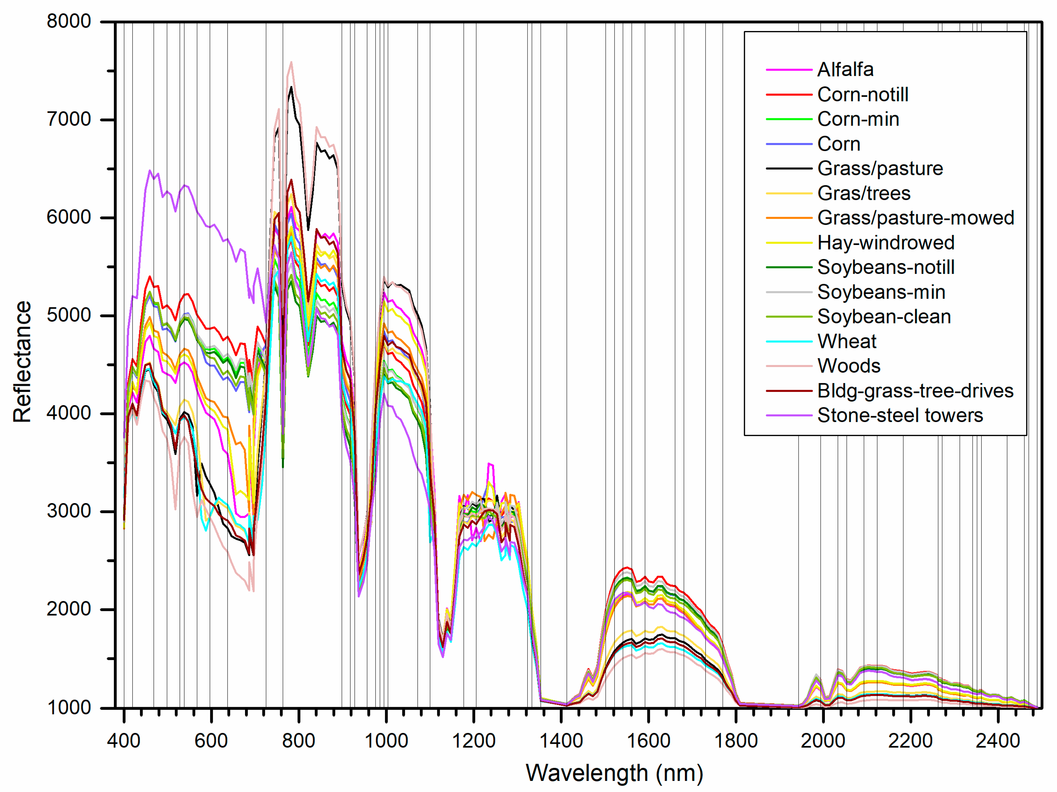
In order to show the position of the eliminated inputs (i.e., spectral bands), mean spectral signatures of 15 LULC classes in the Indian Pines dataset were extracted from the ground reference and the eliminated 53 bands for the 50% sampling ratio were depicted on the figure with vertical lines for further analysis (Figure 6). Perhaps the most striking result is that the proposed method removed the spectral bands adjacent to the previously eliminated noisy bands from the original datasets. It was also noticed that the algorithm detected some spectral ranges (e.g., 764–898 nm, 1004–1071 nm, 1205–1322 nm, 1591–1660 nm) as more beneficial compared to the others for discriminating the LULC classes. However, the spectral bands at the ranges of 918–1004 nm and 1501–1591 nm that indicate similar reflectance measures with the remaining ones were eliminated. Therefore, it can be concluded that the proposed algorithm removed the bands carrying similar information by considering the change or trend in the spectral curves. It is clear from the figure that most of the vegetation types have similar spectral signatures, but they have a varying range of reflectances at blue, green, near-infrared, and shortwave infrared (~1500–1700 nm) regions. The distinct spectral signature of stone-steel towers class can be also noticed.

For the analyses of the OS and FC networks using the test datasets, individual and overall accuracy measures were calculated (

Table 4. Classification accuracies obtained by different training sample sizes for the Indian Pines hyperspectral dataset using fully connected (FC) and optimal superstructure (OS) networks.

Class	10% of Samples			50% of Samples
	Train Pixels	F-Score (FC)	F-Score (OS)	Train Pixels	F-Score (FC)	F-Score (OS)
Alfalfa	22	48.48	64.10	27	77.55	87.27
Corn-notill	144	68.81	74.94	717	78.84	79.77
Corn-min	84	54.30	57.47	417	74.64	70.79
Corn	24	47.72	53.14	117	59.23	64.80
Grass-pasture	50	74.40	76.48	248	88.29	83.86
Grass–trees	75	88.08	87.03	373	92.95	91.72
Grass-pasture-mowed	19	9.92	40.00	13	81.48	92.31
Hay-windrowed	49	90.02	95.34	245	95.35	97.75
Soybean-notill	97	67.00	74.31	484	79.84	79.79
Soybean-min	247	74.84	76.08	1234	84.34	80.97
Soybean-clean	62	54.70	65.03	307	82.93	78.42
Wheat	22	82.90	85.86	106	93.90	92.73
Woods	130	88.54	89.72	647	92.03	92.73
Bldg–Grass–Trees–Drives	38	45.41	62.15	190	67.91	69.54
Stone-Steel towers	19	74.59	81.44	48	95.92	91.11
Overall Acc. (%)		71.98	76.37		83.80	82.72
Kappa		0.680	0.730		0.815	0.802
Weighted kappa		0.715	0.753		0.848	0.850

). While the F-score measure indicating the harmonic mean of user’s and producer’s accuracies was estimated for individual class accuracy assessment, overall accuracy (OA), Kappa, and weighted Kappa coefficients were used to evaluate the accuracy of the thematic maps. When the 10% sampling strategy was employed, the total number of connections in the network decreased from 2,150 to 879, indicating a 61% shrinkage. Although the network was highly compressed, the overall accuracy increased by about 4%, Kappa and weighted Kappa coefficients increased by about 5%. The performance of the FC network dropped, which is obviously a result of the occurrence of overfitting (over 99% overall accuracy on the training data). In the case of OS, the network was prevented from overfitting to training data. On the other hand, for the 50% sampling case, the overall accuracy decreased from 83.80% to 82.72%, indicating only a 1% decrease in the classification performance by decreasing the size of the network by about 66%. Similar results were calculated for Kappa and weighted Kappa coefficients.

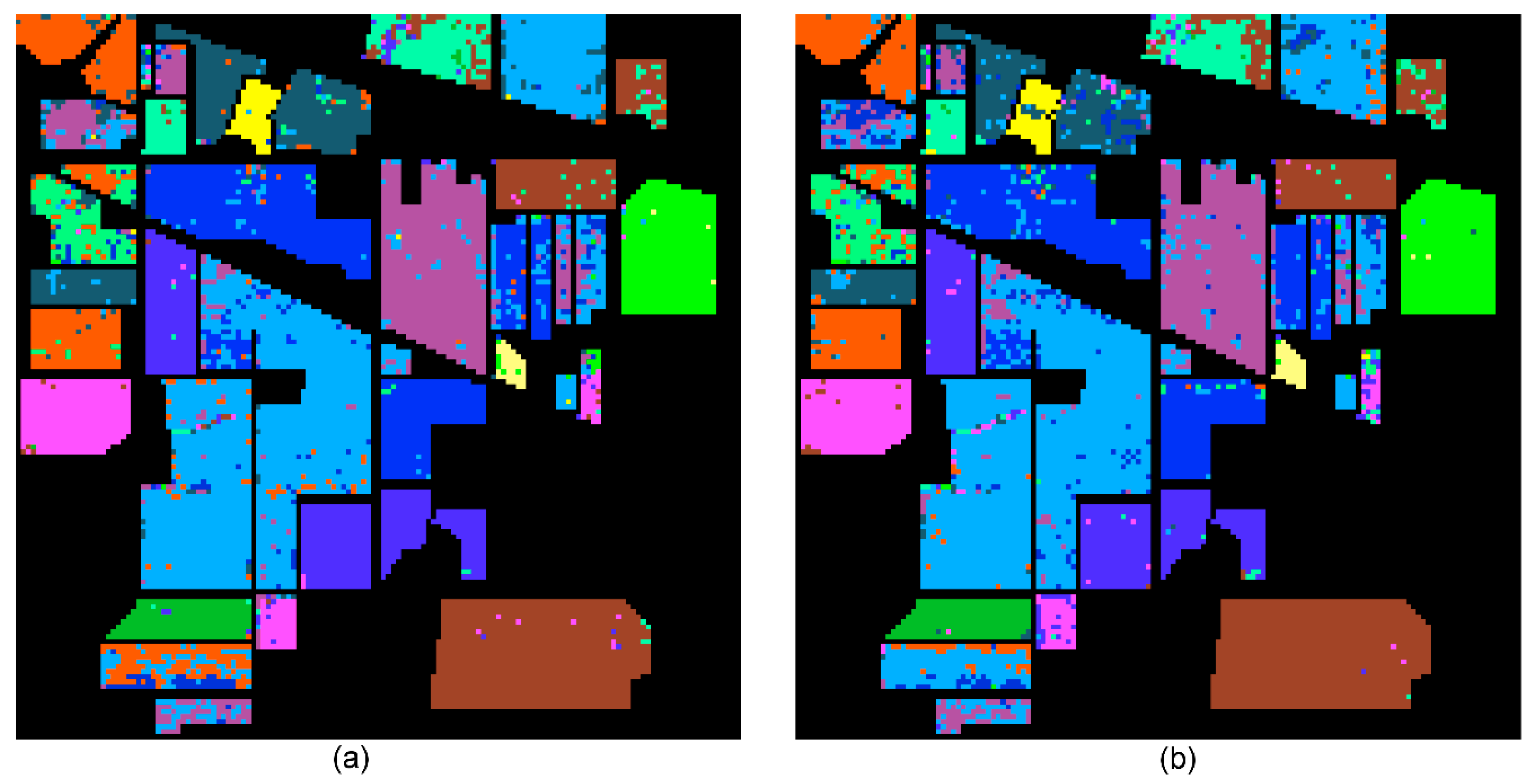
When individual class accuracies estimated for each class were analyzed, some important results were obtained. Firstly, both FC and OS networks produced highly accurate results for some classes, namely grass–trees, hay-windrowed, wheat, woods, and stone-steel towers. However, networks performed poorly for two particular classes, namely corn, and building–grass–trees–drives. The corn class was mostly confused with other corn related classes (i.e., corn-notill and corn-min). The confusion was severe for the fully connected network, producing a 9.92% F-score value for grass-pasture-mowed class, which clearly shows failure in the delineation of this particular cover type. The negative effects of limited and imbalanced data can be easily seen from this class since individual class accuracy varies by about 30% for the 10% sampling case and 11% for the 50% sampling case. The building–grass–trees–drives class covering buildings and their surrounding pervious and impervious features were mainly mixed with the woods class that resulted in a decrease in classification accuracy. Thematic maps produced for the whole dataset using FC and OS networks trained with 50% of whole samples are shown in Figure 7. Misclassified pixels, particularly for the corn related ones, can be easily observed from the comparison of the thematic maps.

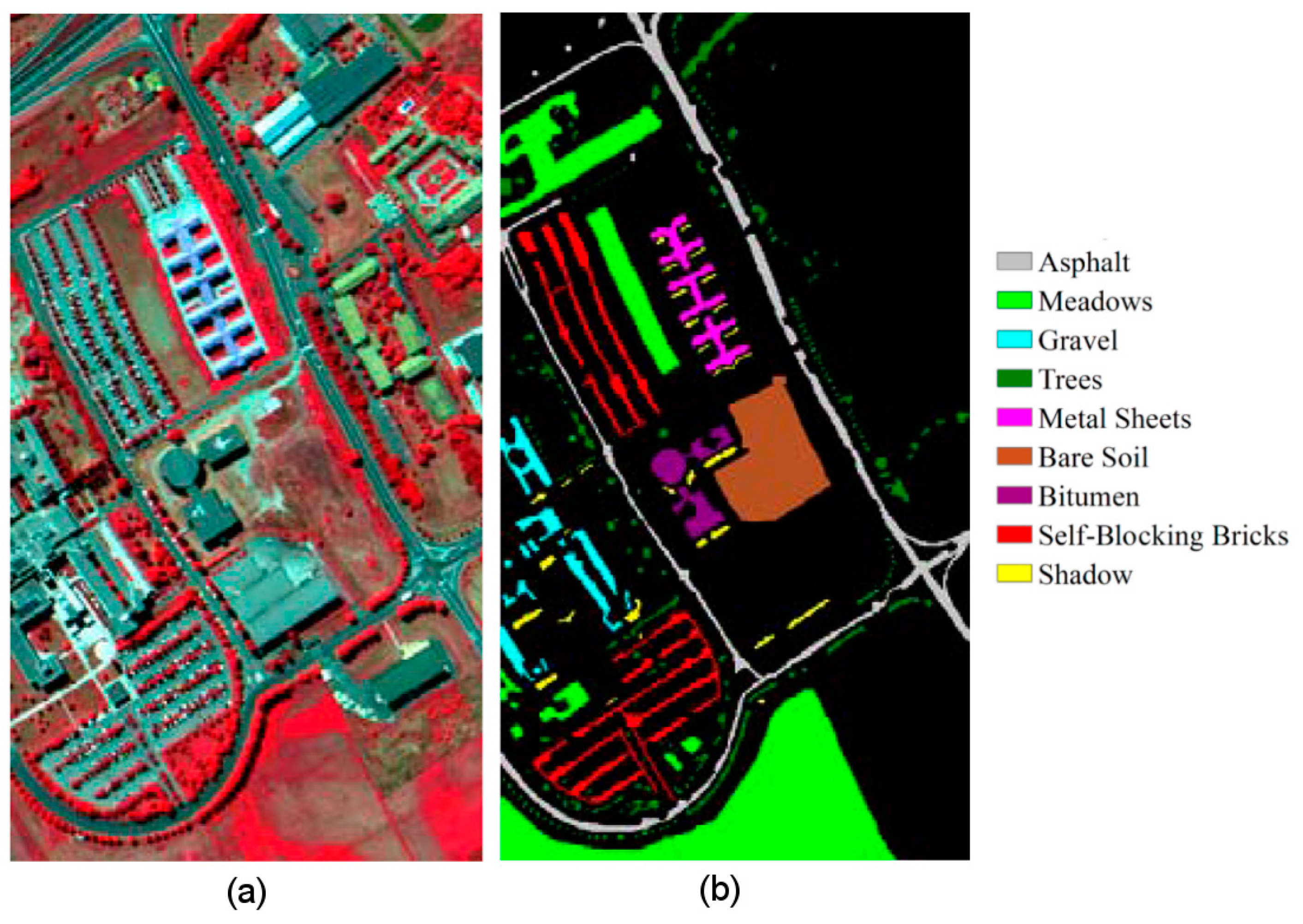
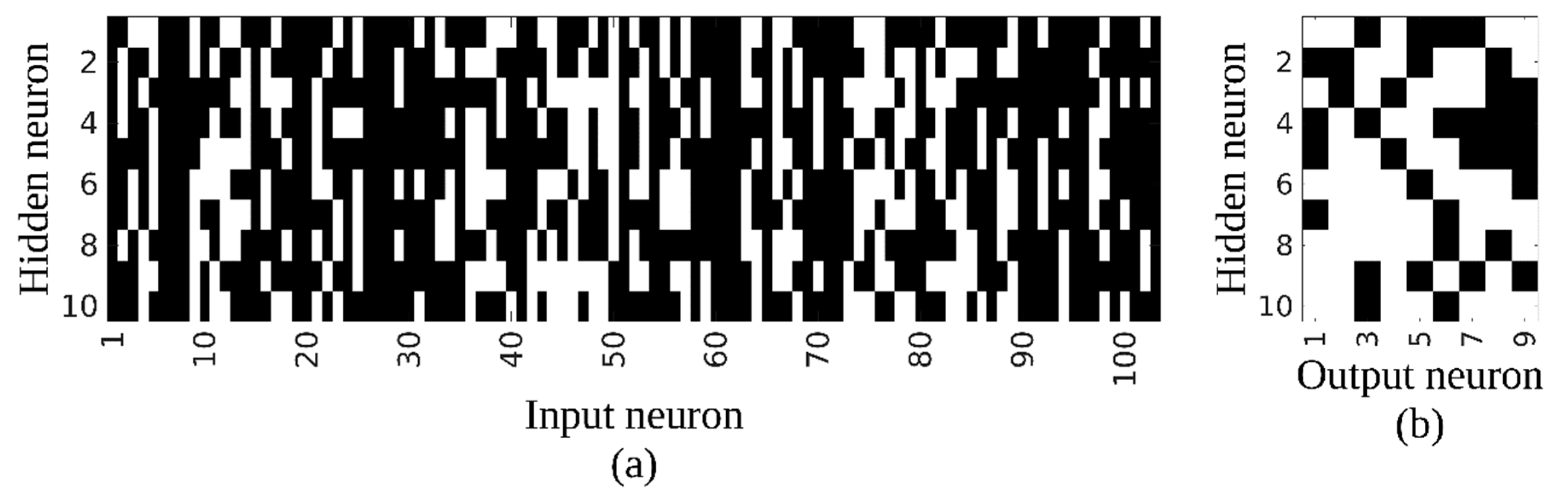
For the Pavia University dataset, a fully connected network of 103-10-9 was optimized throughout the training process to learn the characteristics of the nine LULC classes from 103 spectral bands, and networks of 69-10-9 and 69-7-9 were found optimal in terms of its size and performance for the 10% and 50% sampling ratios, respectively. For the 10% sampling ratio, 697 of 1120 connections were removed from the network, showing a 58% shrinkage. For the 50% sampling ratio, 718 of 1120 links were removed from the network, indicating a 64% shrinkage in the network. For both sampling cases, 34 inputs were removed, indicating a feature selection rate of 33%. In other words, the fully connected network was trimmed by an average of 61%, and 33% of the spectral bands were disregarded as a result of the input selection process. The eliminated and remaining network connections for the 10% sampling ratio were shown in Figure 8. It can be noticed that a comparably smaller number of connections were removed between hidden and output layers, and none of the hidden layer nodes were removed by the proposed algorithm.

Figure 9 shows the final network connections between the layers for the case of the 50% sampling ratio. The removal of three hidden neurons, namely seven, eight, and nine can be easily noticed from the figure (black horizontal lines). Similar to the results produced for the 10% sampling ratio, a smaller number of connections were removed between hidden and output layers.

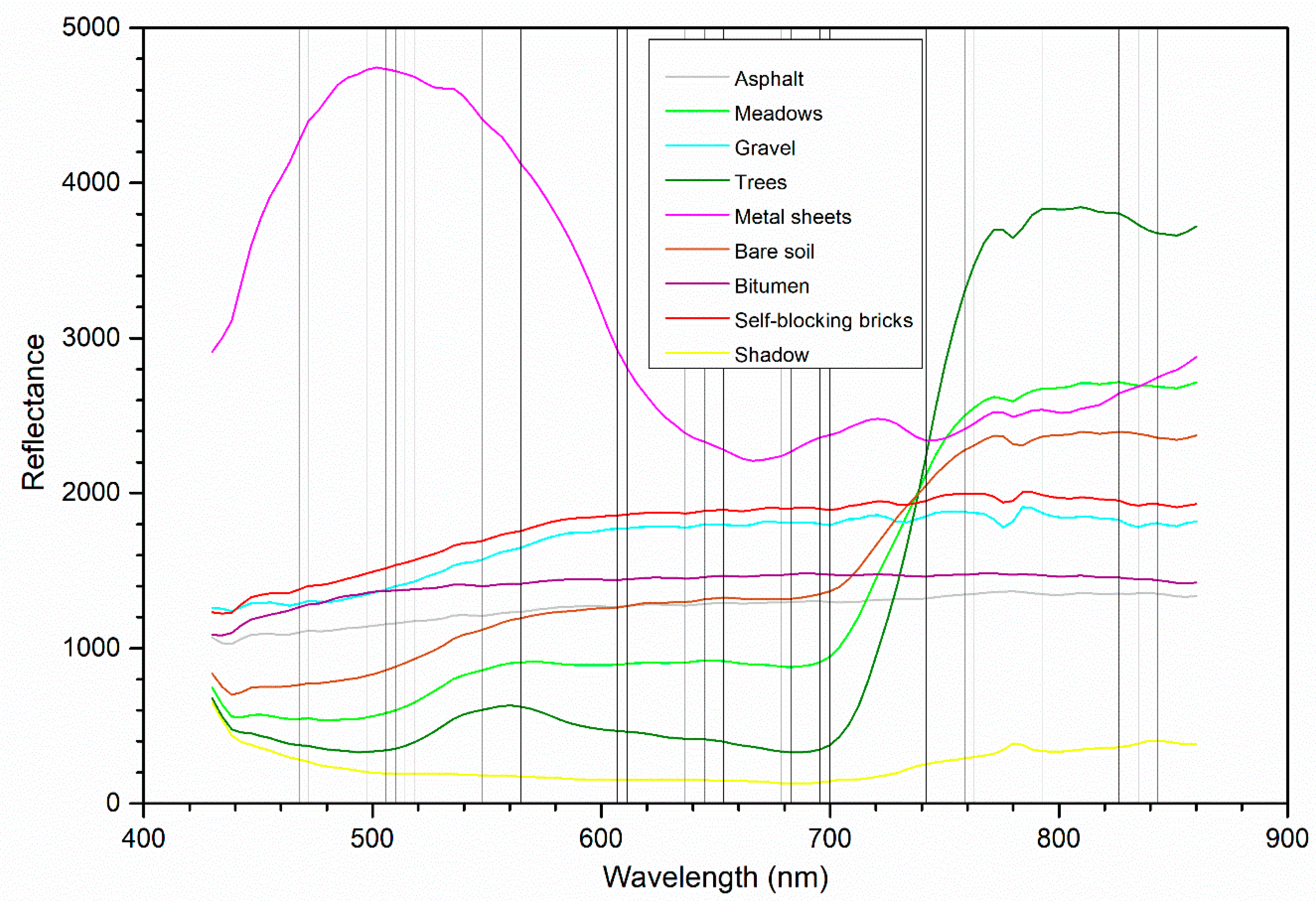
For a clear explanation of the eliminated spectral bands, mean spectral signatures of the classes in Pavia University data were obtained from the ground reference and the location of the eliminated 34 spectral bands for the 50% sampling ratio were shown on the same figure with vertical lines (Figure 10). Similar results with the Indian Pines dataset were observed for the elimination of spectral bands as the highly correlated neighboring bands introducing similar reflectance values were mostly removed from the dataset. The method determines the spectral regions of 573–607, 704–742, and 793–822 nm as discriminating ones for the delineation of the characteristics of the LULC classes. In addition, it removed the spectral bands in the ranges of 468–527 and 607–653 nm. It can be observed that green and red-edge bands were mainly selected for the modeling of the problem. Spectral signature curves also revealed that there were high resemblances between bitumen and asphalt classes, also between gravel and self-blocking bricks classes. Metal sheets and shadow classes had distinct spectral reflectances compared to the other classes. On the other hand, a typical vegetation curve was observed for trees and meadows.

After the training stage for the FC and OS networks, the test data including the rest of the ground reference data for Pavia University were introduced to those networks, and corresponding network performances were presented in

Table 5. Classification accuracies obtained by different training sample sizes for the University of Pavia hyperspectral dataset using FC and OS networks.

Class	10% of Samples			50% of Samples
	Train Pixels	F-Score (FC)	F-Score (OS)	Train Pixels	F-Score (FC)	F-Score (OS)
Asphalt	668	80.24	86.84	3276	90.47	88.56
Meadows	1872	93.18	93.68	9366	95.38	95.07
Gravel	188	65.31	70.87	1032	78.57	72.31
Trees	306	90.28	91.00	1520	93.13	93.48
Painted metal sheets	135	99.34	98.84	670	99.12	99.34
Bare soil	513	75.28	76.47	2529	83.27	80.99
Bitumen	132	62.38	72.23	660	84.66	76.77
Self-blocking bricks	373	70.43	75.03	1860	80.94	77.32
Shadows	91	84.69	91.23	475	94.04	90.85
Overall Acc. (%)		84.63	87.26		90.76	89.21
Kappa		0.796	0.830		0.877	0.856
Weighted kappa		0.813	0.864		0.867	0.871

. With the 10% sampling ratio, the overall accuracy of 87.26%, and a Kappa coefficient of 0.830 were obtained with the optimal superstructure network (OS) while overall accuracy of 84.63% and a Kappa coefficient of 0.796 was achieved by the fully connected network (FC). This clearly shows the robustness of the proposed method, producing about 4% improvement in classification accuracy. With the 50% sampling ratio, the overall accuracy of 89.21% and the Kappa coefficient of 0.856 was obtained with the optimal superstructure network (OS) while the fully connected network (FC) achieved an overall accuracy of 90.76% and Kappa coefficient of 0.877. The accuracy decrease was about 1% for overall accuracy. From these results, it can be stated that the proposed method performs well for a fewer number of samples.

When the individual class accuracies measured by the F-score accuracy measure were analyzed, it was noticed that the lowest accuracies were estimated for the gravel class that was mainly confused with the self-blocking bricks for both FC and OS networks. Similarly, bitumen pixels were confused with asphalt pixels. 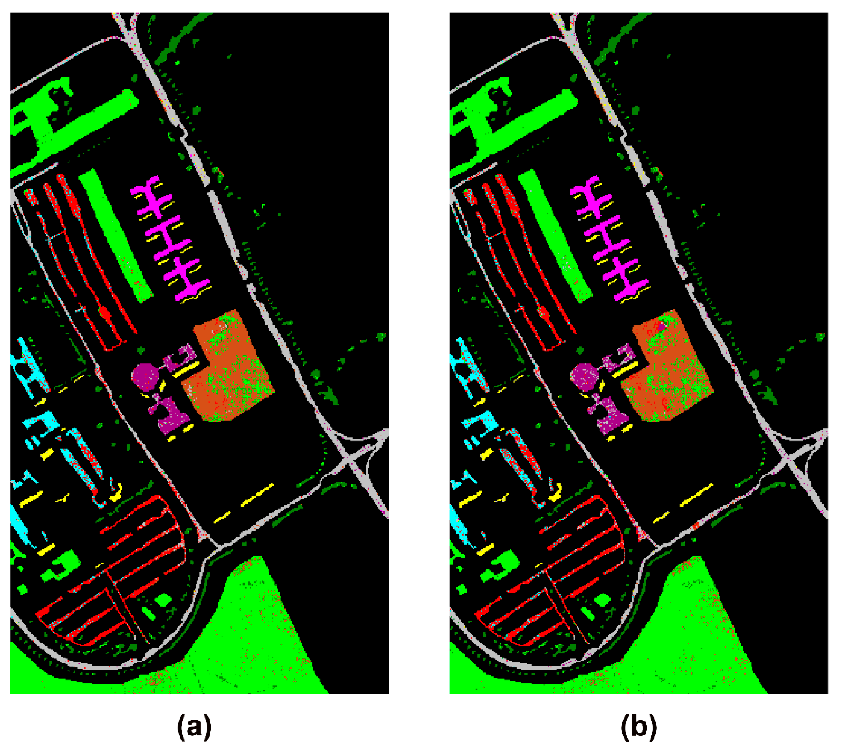This is certainly related to the spectral similarity of the corresponding classes that can be easily observed from the mean spectral reflectance curves (spectral signatures) given in Figure 10. The highest individual class accuracy was achieved for the metal sheets class (over 99%), which has a distinct spectral signature compared to the other classes. The trained networks using the 50% sampling ratio were applied to the whole image to produce the thematic maps of the study, which is presented in Figure 11. Confusion in the class definition for the above-mentioned classes can be observed clearly from the figure. The mixture of gravel and self-blocking bricks pixels is quite obvious in the thematic map produced with the OS network (Figure 11b). Moreover, misclassified pixels within the meadows and asphalt fields are in the form of “salt-and-pepper” noise.

Performances of the FC and OS networks for both datasets were summarized in

Table 6. Performance comparison and network architecture for FC and OS for 10% and 50% samples. Note that OA indicates overall accuracy.

	Indian Pines				Pavia University
	10% Sample		50% Sample		10% Sample		50% Sample
	FC	OS	FC	OS	FC	OS	FC	OS
OA (training)	99.91	97.04	90.37	86.45	99.53	92.10	92.06	90.23
OA (test)	71.98	76.37	83.80	82.72	84.63	87.26	90.76	89.21
$\gamma \sum diag\left(co{v}_p\right)$	6.57	0.08	9.80	0.11	2.34	0.04	1.01	0.03
Number of hidden neurons	10	10	10	9	10	10	10	7
Number of inputs	200	158	200	147	103	69	103	69
Number of connections	2150	879	2150	737	1120	423	1120	402

. For the considered datasets, no hidden neuron was removed from the networks when limited training data (only 10% of the whole datasets) were considered. When the 50% sampling ratio was employed in the training phase, one hidden neuron was eliminated from the FC network for the Indian Pines data and three hidden neurons were removed for the Pavia University data. Smaller networks were found sufficient to learn the underlying characteristics of the LULC classes, and for both cases, the initial networks were trimmed by about 60% in terms of the total number of links, which can be regarded as a success of the proposed algorithm. In addition, a considerable number of inputs (i.e., spectral bands) were removed from the datasets, achieving even better classification performances (about 4% overall accuracy difference). With the implementation of the proposed superstructure optimization, the networks avoided overfitting, thus producing higher classification accuracies for the limited training data (i.e., 10% sampling ratio). It should be mentioned that the FC networks had low generalization capabilities, producing very high accuracy for the training data but comparatively lower accuracies for the test data. The obtained results are promising for the proposed algorithm, being a good alternative to feature selection methods, especially the statistical ones. $\gamma \sum diag\left(co{v}_p\right)$ values in the table indicate the level of overfitting that occurred in the training process. The computed values were much higher for the fully connected networks, particularly the one calculated for the Indian Pines data. Finally, it should be also mentioned that the multiply accumulates (MACS) are directly proportional to the number of connections; therefore, they can be estimated from Table 6.

The comparison of the CPU times of different sampling ratios for the two datasets is given in

Table 7. CPU time comparison for FC and OS for 10% and 50% sampling ratios.

	Indian Pines				Pavia University
	10% Sampling		50% Sampling		10% Sampling		50% Sampling
	FC	OS	FC	OS	FC	OS	FC	OS
Training (s)	41.5	7213	65.3	10823	40.2	5418	63.7	9036
Test (s)	0.015	0.010	0.007	0.005	0.05	0.03	0.02	0.01

. All the results were obtained using an Intel Core i5-6400 CPU 2.7 GHz 4 core 16 Gb RAM machine using a Linux operating system. It was observed that the CPU times of the proposed training method were larger than the FCs because of the MINLP programs. MINLPs are known to be NP-hard and cannot be solved in polynomial time, whereas standard training algorithms (NLPs) are P-only types. Therefore, the required computational time can be much higher for the proposed method. On the other hand, reduced and optimal ANN structures should result in faster CPU times since the number of required multiplication operations is much lower, which might also be a beneficial feature for testing larger ANNs, e.g., deep neural networks.

5. Conclusions

This study investigates the optimal training of multi-layer perceptrons through formulating and solving a mixed-integer non-linear optimization problem, delivering a significant reduction in the number of network connections, neurons, and input variables. It differs from the other methods proposed in literature as it introduces both a strong and general mixed-integer programming method for optimal structural design and allows automatic and simultaneous design and training. This feature is particularly advantageous since the presence of redundant inputs and connections decreases the prediction performance of the ANNs and increases the computational load for training. Furthermore, classical input selection (i.e., feature selection) and pruning methods, including dropout layers into deep neural networks, usually require many sequential iterations between design and training instead of automatic and simultaneous design and training. Two classification case studies with two sampling ratios (10% and 50% sampling ratios), namely Indian Pines and Pavia University datasets, were considered as benchmark test sites, and the results showed that optimal ANN structures contained a significantly lower number of inputs, connections, and neuron numbers. To be more specific, although about 60% of the network connections and 25% of the inputs (i.e., spectral bands) were removed by the proposed algorithm, superior classification performances (~4% in terms of overall accuracy) were achieved with the estimated optimal superstructure for the case of limited training samples (10% of the whole samples). It was observed that the method eliminated the least effective and correlated spectral bands that have an insignificant or trivial contribution to the delineation of the LULC characteristics. To the best of authors’ knowledge, this paper is the first application of such an automatic and optimal design and training method for MLP type neural networks for classification problems. Finally, the method presented in this work can be applied using global optimization algorithms for further enhancement in terms of the prediction performance of ANNs. Moreover, reduced and optimal ANN structures should result in faster CPU times, since the number of required multiplication operations is much smaller, which could be a beneficial feature for testing larger ANNs, e.g., deep neural networks.