Abstract
This study proposes a deep quadruplet network (DQN) for hyperspectral image classification given the limitation of having a small number of samples. A quadruplet network is designed, which makes use of a new quadruplet loss function in order to learn a feature space where the distances between samples from the same class are shortened, while those from a different class are enlarged. A deep 3-D convolutional neural network (CNN) with characteristics of both dense convolution and dilated convolution is then employed and embedded in the quadruplet network to extract spatial-spectral features. Finally, the nearest neighbor (NN) classifier is used to accomplish the classification in the learned feature space. The results show that the proposed network can learn a feature space and is able to undertake hyperspectral image classification using only a limited number of samples. The main highlights of the study include: (1) The proposed approach was found to have high overall accuracy and can be classified as state-of-the-art; (2) Results of the ablation study suggest that all the modules of the proposed approach are effective in improving accuracy and that the proposed quadruplet loss contributes the most; (3) Time-analysis shows the proposed methodology has a similar level of time consumption as compared with existing methods.
1. Introduction
A hyperspectral image covers hundreds of bands with high spectral resolution and provides a detailed spectral curve for each pixel [1,2]. Both the spatial and the spectral information are gathered in a hyperspectral image. Hyperspectral image classification is aimed at identifying the specific class (i.e., label) for each pixel (for example, cropland, lake, river, grassland, forest, mineral rocks, building, and roads). As the first step in many hyperspectral remote sensing applications, image classification is vital in the fields of agricultural statistics, disaster reduction, mineral exploration, and environmental monitoring.
In recent decades, many methods have been proposed for the hyperspectral image classification, such as spectral angle mapper (SAM), mixture tuned matched filtering (MTMF), spectral feature fitting (SFF) [3,4], neural network (NN) [5], support vector machine (SVM) [6,7], and random forest (RF) [8,9]. SAM, MTMF, and SFF are heavily influenced by anthropogenic decision-making, while NN, SVM, and RF are gradually becoming more dependent on new machine learning methods. Since the concept of deep learning was introduced into hyperspectral image classification for the first time [10], deep neural network has been gaining popularity and has triggered global research interest in establishing deep learning models for hyperspectral image classification [11,12,13,14]. In particular, some deep-learning methods have been proposed by combining spectral and spatial features to improve classification accuracy [15,16,17,18,19,20,21].
However, the aforementioned methods still require substantial improvements in hyperspectral image classification, especially under the condition of small-samples. For supervised classification of remotely sensed images, the training samples are usually acquired by two methods: (1) from field surveys and (2) directly from images with higher resolution. In particular, higher classification accuracy is usually acquired from training samples collected by field surveys. However, compared with laboratory work, field survey is costly, complicated, and time-consuming, which can significantly restrict the number of training samples. A small dataset of training samples can substantially diminish accuracy in hyperspectral image classification. Moreover, hyperspectral images suffer more from data redundancy in the spectral dimension compared with multi-spectral images, which creates additional difficulties for classification.
Few-shot learning involves solving the problem using a limited number of samples and has been used for various applications such as image segmentation, image caption, object recognition, and face identification. [22,23,24,25]. Given the limited accuracy due to having only a few labeled samples per class, few-shot learning usually trains the model based on a well-labeled dataset, and the model is then generalized into new classes [26]. A metric learning strategy is usually adopted to learn the features of the object and distinguish based on the absolute distance between samples [27]. In recent years, several few-shot learning methods have been proposed for hyperspectral image classification, e.g., DFSL (deep few-shot learning) [28,29]. However, absolute distance ignores the relationship between inter-class and intra-class and limits classification accuracy. The use of relative distance, based on widening inter-class distance and shortening the intra-class distance, has been proposed in lieu of absolute distance [30]. Proposing new methods that account for the relative relationship between inter-class and intra-class is therefore crucial in improving the accuracy of hyperspectral image classification with a limited number of samples.
This study proposes a deep quadruplet network (DQN) for hyperspectral image classification with a small number of samples. To improve the accuracy, we designed a quadruplet network, in particular, a new quadruplet loss function, and a deep 3-D CNN with double branches consisting of dense convolution and dilated convolution.
2. Materials and Methods
2.1. Data
2.1.1. Training Data
The training data used in this study are four well-known public hyperspectral datasets: “Houston”, “Chikusei”, “KSC”, and “Botswana” [28]. The details of the four hyperspectral datasets used in training are presented in Table 1.

Table 1.
The details of the four hyperspectral datasets for training networks [28].
2.1.2. Testing Data
The testing data used in this study are three widely-known public hyperspectral datasets: “Salinas”, “Indian Pines” (IP), and “University of Pavia” (UP). The details of the three hyperspectral datasets used in testing are summarized in Table 2. The ground-truth maps of the three hyperspectral datasets are shown in Figure 1, Figure 2 and Figure 3.
Table 2.
The details of the three hyperspectral datasets for testing networks [28].
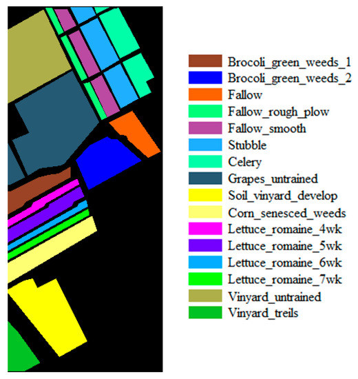
Figure 1.
Ground-truth map of the Salinas dataset.
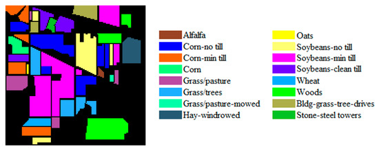
Figure 2.
Ground-truth map of the Indian Pines (IP) dataset.
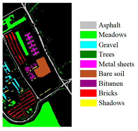
Figure 3.
Ground-truth map of the UP dataset.
The training datasets “Houston” and “Chikusei” can be acquired from the following websites, respectively: “http://hyperspectral.ee.uh.edu/2egf4tg8hial13gt/2013_DFTC.zip” and “http://park.itc.u-tokyo.ac.jp/sal/hyperdata/Hyperspec_Chikusei_MATLAB.zip”. The training datasets “KSC” and “Botswana” and all the testing datasets can be acquired from the website “http://www.ehu.eus/ccwintco/index.php?title=Hyperspectral_Remote_Sensing_Scenes”.
2.2. Structure of the Proposed Method
The structure of the proposed methodology in this study is shown in Figure 4. A deep quadruplet network is trained to learn a feature space. The testing data is transferred to the learned feature space to extract features. The classification is accomplished using the Euclidean distance and the nearest neighbor (NN) classifier.
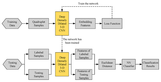
Figure 4.
The structure of the proposed methodology.
2.3. Quadruplet Learning
Metric learning refers to the transfer of input data from the original space RF into a new feature space RD (i.e., fθ: RF→RD). F and D refer to the dimension of the original space and the new space, respectively, and θ is the learnable parameter. In the new feature space RD, samples from the same class are expected to be closer than those from different classes so that the classification can be finished in RD using nearest neighbor classifier. Several networks have been developed to accomplish this task, including the siamese network, triplet network [31], and quadruplet network [32].
In a siamese network, a contrastive loss function is designed to train the network to distinguish between pairs of samples from the same class and those from different classes. The designed loss function limits the samples within the same class and enlarges the samples from the different classes. However, for classification purposes, the feature space learned by the siamese network is inferior to that of the triplet network. In addition, siamese networks are sensitive to calibration in order to contextualize similarity vs. dissimilarity [31]. The loss function for a siamese network is:
where xa(i) and xp(i) are two samples from the same class, which has been transferred by fθ: RF→RD; Ns is the number of siamese pairs; and d (·) is the Euclidean distance of two elements.
Triplet network refers to training based on the use of many triplets. A triplet contains three different samples (xa(i), xp(i), xn(i)), where xa(i) and xp(i) are two samples from the same class (i.e., positive pairs), while xa(i) and xn(i) are samples from different classes (i.e., negative pairs). Each sample in a triplet has been transferred by fθ: RF→RD. The loss function for the triplet network is given by [32]:
where γ is the value of the margin set that segregates the positive pairs with the negative pairs; Nt is the number of triplets; and (z)+ = max (0, z). The first term is intended to shorten the distance between two samples from the same class, while the second term is designed to enlarge the distance between two samples from different classes. For the loss function in triplet networks, each positive pair and negative pair share a given sample (i.e., xa(i)), which compels triplet networks to focus more on obtaining the correct ranks for the pair distances. In other words, the triplet loss only considers the relative distances of the positive and negative pairs, which results in poor generalization for the triplet network and difficulty applying in tracking tasks [32].
The quadruplet loss (QL) [30] introduces a different negative pair into the triplet loss. The quadruplet loss function contains four different samples: (xa(i), xp(i), xn1(i), xn2(i)), where xa(i) and xp(i) are samples from a same class while xn1(i) and xn2(i) are samples from another two classes. All the samples have been transferred to the featured space by fθ: RF→RD. The quadruplet loss is given by the equation:
where γ and β are the margins for the two terms; and Nq is the number of quadruplets. The first term in quadruplet loss is the same as that in the triplet loss (Equations (2) and (3)). The second term constrains the intra-class distances to be smaller than the inter-class distances [30]. However, the loss function in Equation (3) usually performs poorly because the number of quadruplets and quadruplet pairs would grow rapidly when the dataset gets more extensive. Moreover, most samples are not so useful towards adequately training the network and can overwhelm the relevant hard-learning samples, leading to the poor performance of the network [32].
Hence, this study designed a new quadruplet loss function, as shown in Equation (4):
where xp(i) is the farthest sample to the reference xa(i) in the same class; xm(i) and xn(i) are the closest negative pairs in the whole batch; Nnq is the number of quadruplets in the new loss function; and γ is the value of the margin. Each sample in Equation (4) has been transferred by fθ: RF→RD. The conceptual diagram of the quadruplet network, as proposed in this study, is presented in Figure 5. The proposed loss function compensates for the shortcomings of Equations (2)–(4). The procedure for batch training using the proposed loss function is shown in Table 3, where T= {t1, t2, t3, …, ts} is the training dataset for this batch, and s is the number of labeled samples. In a batch (shown in Table 3), Nnq = s, and tj or tk represents a sample in the dataset T. (tj, tk) represents a pair of samples, C (tj) is the class label of the sample tj, and α is the learning rate. The variables ta, tp, tm, and tn are the quadruplets before the deep network, while xa, xp, xm, and xn are the corresponding quadruplets after the deep network.
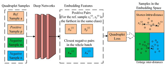
Figure 5.
The concept of the quadruplet network proposed in this study.
Table 3.
The procedure for training a batch.
2.4. Deep Dense Dilated 3-D CNN
2.4.1. Deep Network Framework
As shown in Figure 6, the overall framework of the proposed deep dense dilated 3-D CNN contains two branches: a dense CNN and a dilated CNN.
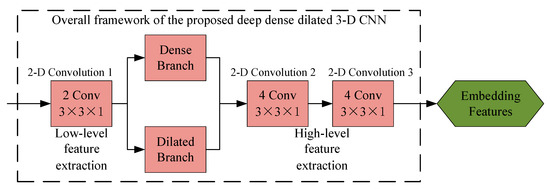
Figure 6.
The overall framework of the proposed deep dense dilated 3-D convolutional neural network (CNN).
2.4.2. Dense CNN
The dense CNN block consists of five convolutional layers (see Figure 7a). “Conv” is a convolutional operation with a 3 × 3 × 3 kernel, while “2 Conv” represents a convolutional layer with two kernels (i.e., two convolutional operations). For a normal CNN block with five layers, there are five connections (a connection is between a layer and its subsequent layer) [33] (see Figure 7b). However, as the network becomes more and more deep, the problem with a normal CNN is that the features contained in the input can vanish after it passes through many layers until it reaches the end [33]. So instead of using the normal CNN, a dense CNN was used in this study. Aside from the preserving the five connections from the normal CNN block, the dense CNN provides six other connections: three connections are between the 1st layer and the 3rd, 4th, and 5th layers; two connections are between the 2nd Conv and the 4th and 5th Conv; and one connection is between the 3rd Conv and the 5th Conv. Figure 7a shows the operation at a connection point in the dense CNN, and “⊕” represents the sum of all the imported connected lines.
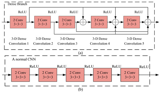
Figure 7.
The dense CNN block in this study and a normal CNN block. (a) The structure of the dense CNN block with 5 layers in this study; (b) a normal CNN block with 5 layers.
The use of the dense CNN in this study alleviates the problem regarding information vanishing when passing through numerous layers and make full use of the features extracted by all the layers.
2.4.3. Dilated CNN
For normal convolutional operation, the convolutional kernel covers an image area using the same size (Figure 8a). A normal CNN employed in image classification represents the image using many tiny feature scenes, resulting in obscure spatial structures [34]. Moreover, the spatial acuity and details that are lost are almost impossible to restore through upsampling and training. Hence, the image classification accuracy is limited using the normal CNN, especially for images requiring detailed scene understanding [34]. Dilated convolution is an operation in which the convolutional kernel covers an image area with a bigger size (Figure 8b). For example, a 3 × 3 convolutional kernel only covers a 3 × 3 image area in normal convolutional operation (Figure 8a), but a 3 × 3 convolutional kernel can enlarge the receptive field to 5 × 5 (Figure 8b), or even bigger field. The dilated CNN represents the image features on a bigger scale and alleviates the disadvantage of data redundancy in a hyperspectral dataset without increasing the network’s depth or complexity [34]. The structure of the dilated branch in this study is shown in Figure 9.
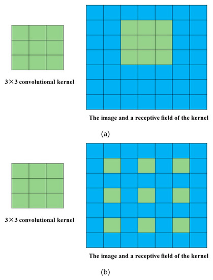
Figure 8.
The convolutional operation in a normal and dilated CNN. (a) The convolutional operation in a normal CNN using a 3 × 3 convolutional kernel; (b) the convolutional operation in a dilated CNN using a 3 × 3 convolutional kernel.
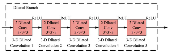
Figure 9.
The structure of the dilated branch in this study.
In both the dense CNN block and the dilated CNN block, there is an operation called ReLU. ReLU is an activation function defined as:
f(x)=max(0, x)
2.5. Nearest Neighbor (NN) for Classification
In this study, an embedded feature space is learned after training the proposed deep quadruplet CNN using the training data. For the testing data, the supervised samples and the samples to be classified are transferred to the embedded feature space by the trained deep quadruplet CNN. The classification is completed using the average Euclidean distance between the supervised samples and the samples to be classified using the nearest neighbor classifier.
2.6. Parameters Setting
Details of the network architecture for the proposed deep quadruplet network are summarized in Table 4. The layer names in Table 4 correspond with the blocks in Figure 6, Figure 7, and Figure 9. N is the band number of the hyperspectral dataset. The N bands are selected by graph representation based band selection (GRBS) [35]. “ceil (N/2)” is the ceiling function, which is equal to the rounded-up integer of N/2. The learning rate α for optimizing DQN is set to be 10-3 with a weight decay of 10-4 and a momentum of 0.9. The sensitivity of the margin γ to the classification accuracy was tested with 15 supervised samples per class. The overall accuracy (OA) for all three testing datasets is shown in Figure 10. The value of γ was set to be 0.4, which refers to the best accuracy obtained for all the three testing datasets, as presented in Figure 10.
Table 4.
The network architecture details of the proposed deep quadruplet network.
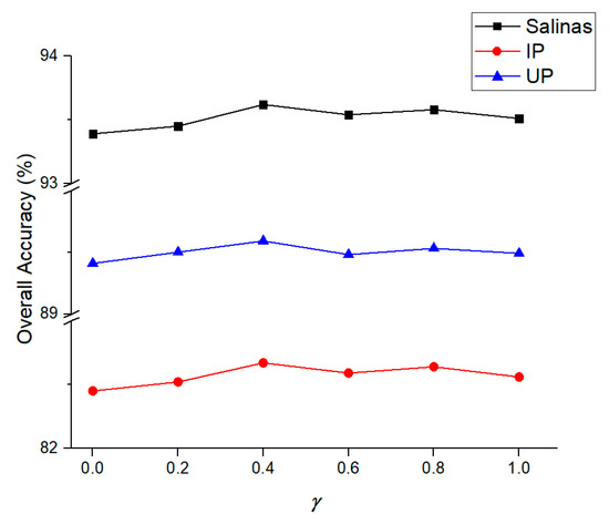
Figure 10.
The overall accuracy with different γ for all the three testing datasets.
3. Results and Discussion
3.1. Accuracy
For the Salinas and the UP datasets, the number of supervised samples (L) used in the testing experiments was set to 5, 10, 15, 20, and 25. Given the limited total number of labeled samples in the IP dataset, the number of supervised samples (L) used in the testing experiments was set to 5, 10, and 15. For each case of L, the supervised samples are selected randomly and ten runs were performed. The overall accuracy of each run was recorded. The results of the classification using the proposed method (DQN+NN) are presented in Figure 11, Figure 12 and Figure 13. The overall accuracy of the proposed approach was then compared with other methods, including: SVM [6], LapSVM [36], TSVM [37], SCS3VM [38], SS-LPSVM [39], KNN+SNI [40], MLR+RS [41], SVM+S-CNN, 3D-CNN [19], DFSL+NN, and DFSL+SVM [28]. The average value and the standard deviation (STD) of the overall accuracy in the ten runs for the three testing datasets using the different methods are shown in Table 5, Table 6 and Table 7. The overall accuracy of 3D-CNN was examined based on the method described by Hamida et al. [19]. The accuracy of the SVM, LapSVM, TSVM, SCS3VM, SS-LPSVM, KNN+SNI, MLR+RS, SVM+S-CNN, DFSL+NN, and DFSL+SVM are derived from the study of Liu et al. [28]. The training datasets and testing datasets in our paper are exactly same with that in Reference [28], which are public and have been widely used for comparing different methods for hyperspectral image classification [28,38,39,40,41]. Hence, the comparison of different methods is appropriate.
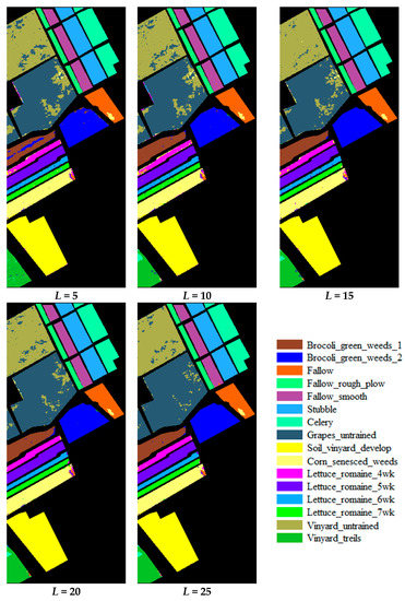
Figure 11.
The classification results of the Salinas dataset.
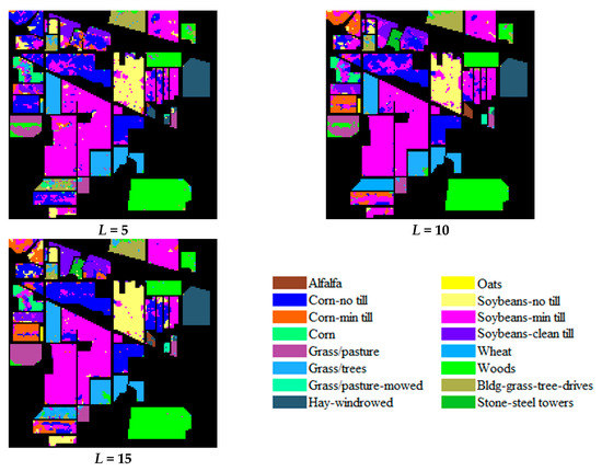
Figure 12.
The classification results of the IP dataset.
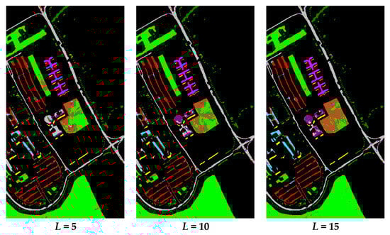
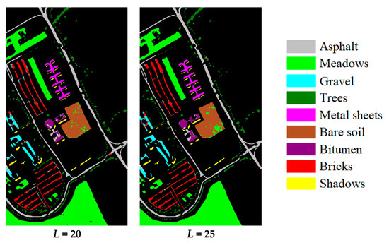
Figure 13.
The classification results of the University of Pavia (UP) dataset.
Table 5.
The average ± STD overall accuracy (OA, %) with Salinas dataset using different methods (The bold value is the best accuracy in each case).
Table 6.
The average ± STD overall accuracy (OA, %) with IP dataset for different methods (The bold value is the best accuracy in each case).
Table 7.
The average ± STD overall accuracy (OA, %) with UP dataset for different methods (The bold value is the best accuracy in each case).
Table 5, Table 6 and Table 7 show that the accuracy of the proposed method with different numbers of supervised samples is better compared to other methods in all three testing datasets. From Table 5, Table 6 and Table 7, it can be inferred that the proposed method is state-of-the-art for few-shot hyperspectral image classification in terms of classification accuracy.
There are some other results reported in existing publications [28]. The OA could reach 97.81%, 98.35%, and 98.62% for Salinas, IP, and UP dataset, respectively [28]. However, these results are obtained based on 200 supervised samples per class (L = 200). It is obvious that more supervised samples lead to better accuracy. Our paper pays attention to the hyperspectral image classification with a small number of samples, so the situation with L = 200 is out of our discussion.
Here is an explanation about the generalization of the network from some classes to new classes. Traditional artificial neural network has been successful in data-intensive applications, but it is hard to learn from a limited number of examples. To solve this problem, few-shot learning (FSL) is proposed [42]. Few-shot learning (FSL) is a type of machine learning problems where there is a little supervised information for the target. A strategy is that the network learns prior knowledge, and it can be generalized to new tasks with limited supervised samples. In fact, it is an important and famous branch of machine learning and has been widely used to solve many problems [28,32,42] (e.g., face recognition). The feature space learned from hyperspectral image has been demonstrated the ability to generalize to the new classes [28]. The network trained in this paper is also essentially a generalized feature extractor. The extracted features of supervised samples and samples to be classified are put into the classifier (nearest neighbor) to finish the classification.
Here we make it clear that the L specific supervised samples are not exactly the same as those in [28], due to the randomness of selecting supervised samples. However, the way of selection of supervised samples and comparative analysis in this paper is the same as that in [28,39]. It is common to randomly select supervised samples and conduct several runs of experiments (e.g., 10 runs in [28,39], and also our paper). The purpose is to avoid the occasionality of accuracy in one run.
3.2. Ablation Study
There are three key modules in the proposed methodology: the quadruplet loss, the dense branch, and the dilated branch. To demonstrate the effectiveness of each module, the classification accuracy was calculated when one of the modules is replaced. Simply put, an ablation study was performed. The proposed quadruplet loss was replaced by the siamese loss, the triplet loss, and the original quadruplet loss. The dense branch or dilated branch was replaced using a normal CNN module. In the proposed methodology, when one module is replaced, the other modules are kept the same. The summary of average values ± STD of OA in the ten runs is shown in Table 8, Table 9 and Table 10 for all three testing datasets.
Table 8.
The OA of the Salinas dataset when the modules are replaced.
Table 9.
The OA of the IP dataset when the when the modules are replaced.
Table 10.
The OA of the UP dataset when the modules are replaced.
In every method where a module was replaced, the accuracy was lower compared with the proposed methodology (see Table 8, Table 9 and Table 10). The inclusion of the quadruplet loss, the dense branch, and the dilated branch contributes to improving the accuracy, which was demonstrated by the ablation study. In particular, the decrease in accuracy was most substantial when the quadruplet loss was replaced, which suggests that the designation of the quadruplet loss contributes the most in improving the accuracy in the proposed methodology.
Table 11, Table 12 and Table 13 shows the average accuracy (AA) and Kappa coefficients of the proposed method, 3D-CNN, and the five experiments in ablation study. There is no enough information in publications for other existing methods. Table 11, Table 12 and Table 13 suggest that the proposed method obtains satisfying results in terms of average accuracy and Kappa coefficient.
Table 11.
The average accuracy (AA, %) and the Kappa coefficient (%) for Salinas dataset.
Table 12.
The average accuracy (AA, %) and the Kappa coefficient (%) for IP dataset.
Table 13.
The average accuracy (AA, %) and the Kappa coefficient (%) for UP dataset.
3.3. Time Consumption
In terms of the overall accuracy of the three datasets, SS-LPSVM, 3D-CNN, DFSL+NN, and DFSL+SVM show the closest accuracy performance with our method. Hence, these methods were selected for the comparative analysis of time consumption. The time consumption of 3D-CNN, DFSL+NN, DFSL+SVM, and the proposed method based on the IP dataset is shown in Table 14. Details regarding the computer configuration and program coding used in analyzing the time consumption are presented in Table 15. Based on the comparative analysis of time consumption, the proposed approach is similar to other classification techniques. SS-LPSVM has been demonstrated that it takes much longer time than DFSL+NN and DFSL+SVM based on the IP dataset [28] (198.30s vs. 11.14s + 0.36s and 11.14s + 2.21s). Hence, it can be inferred that the proposed method shows obvious advantage over SS-LPSVM.
Table 14.
The time consumption of the proposed approach and other methods (“+”: the time of feature extraction + the time of classification).
Table 15.
The details about computer configuration and program coding for testing operation time.
4. Conclusions
This study integrates quadruplet loss with deep 3-D CNN with dense and dilated characteristics in proposing a quadruplet deep learning method for few-shot hyperspectral image classification. Verification and comparative analysis were performed using public hyperspectral datasets, and the results suggest the following conclusions:
(1) The proposed approach was found to have higher overall accuracy than existing methods, which suggests that the classification method is state-of-the-art.
(2) An ablation study was conducted replacing each module of the proposed approach (i.e., quadruplet loss, dense branch, and dilated branch) to demonstrate the effectiveness of their contributions. The results show that all modules are effective and necessary in improving classification accuracy, with the proposed quadruplet loss providing the highest contribution.
(3) The time consumption for the different methods was tested under the same operating environment. The analysis shows the proposed methodology has a similar level of time consumption compared to existing methods.
In the future, given the scarcity of training samples in some cases, a sample-synthesis method can be explored for a few-shot hyperspectral image classification.
Author Contributions
C.Z. and J.Y. together proposed the idea and contributed to the experiments, writing, and figures, and contributed equally to this work; Q.Q. contributed to the writing of this paper. All authors have read and agreed to the published version of the manuscript.
Funding
This research was funded by National Natural Science Foundation of China (Grant number 41901291), National key research and development program (Grant number 2018YFC1800102), Open Fund of State Key Laboratory of Coal Resources and Safe Mining (Grant number SKLCRSM19KFA04), the Key Laboratory of Surveying and Mapping Science and Geospatial Information Technology of Ministry of Natural Resources (Grant number 201917), the Key Laboratory for National Geographic Census and Monitoring, National Administration of Surveying, Mapping and Geoinformation (Grant number 2018NGCM07).
Acknowledgments
The authors gratefully acknowledge the National Center for Airborne Laser Mapping (NCALM) for providing the “Houston” dataset, the Space Application Laboratory, Department of Advanced Interdisciplinary Studies, University of Tokyo for providing the “Chikusei” dataset, and Grupo de Inteligencia Computacional (GIC) for providing other datasets. The authors thanks to the professional English editing service from EditX.
Conflicts of Interest
The authors declare no conflict of interest.
References
- Magendran, T.; Sanjeevi, S. Hyperion image analysis and linear spectral unmixing to evaluate the grades of iron ores in parts of Noamundi, Eastern India. Int. J. Appl. Earth Obs. Geoinf. 2014, 26, 413–426. [Google Scholar] [CrossRef]
- Zhang, C.; Qin, Q.; Chen, L.; Wang, N.; Zhao, S.; Hui, J. Rapid determination of coalbed methane exploration target region utilizing hyperspectral remote sensing. Int. J. Coal Geol. 2015, 150, 19–34. [Google Scholar] [CrossRef]
- Kruse, F. Preliminary results—Hyperspectral mapping of coral reef systems using EO-1 Hyperion. In Proceedings of the 12th JPL Airborne Geoscience Workshop, Buck Island and U.S. Virgin Islands, Buck Island, USVI, USA, 24–28 February 2003. [Google Scholar]
- Van der Meer, F.D.; Van der Werff, H.M.A.; Van Ruitenbeek, F.J.A.; Hecker, C.A.; Bakker, W.H.; Noomen, M.F.; van der Meijde, M.; Carranza, E.J.M.; de Smeth, J.B.; Woldai, T. Multi- and hyperspectral geologic remote sensing: A review. Int. J. Appl. Earth Obs. Geoinf. 2012, 14, 112–128. [Google Scholar] [CrossRef]
- Benediktsson, J.A.; Swain, P.H.; Ersoy, O.K. Neural Network Approaches Versus Statistical Methods in Classification of Multisource Remote Sensing Data. In Proceedings of the 12th Canadian Symposium on Remote Sensing Geoscience and Remote Sensing Symposium, Vancouver, BC, Canada, 10–14 July 1989; pp. 489–492. [Google Scholar]
- Melgani, F.; Bruzzone, L. Classification of hyperspectral remote sensing images with support vector machines. IEEE Trans. Geosci. Remote Sens. 2004, 42, 1778–1790. [Google Scholar] [CrossRef]
- Gao, L.; Li, J.; Khodadadzadeh, M.; Plaza, A.; Zhang, B.; He, Z.; Yan, H. Subspace-Based Support Vector Machines for Hyperspectral Image Classification. IEEE Geosci. Remote Sens. Lett. 2015, 12, 349–353. [Google Scholar]
- Ham, J.; Chen, Y.C.; Crawford, M.M.; Ghosh, J. Investigation of the random forest framework for classification of hyperspectral data. IEEE Trans. Geosci. Remote Sens. 2005, 43, 492–501. [Google Scholar] [CrossRef]
- Gislason, P.O.; Benediktsson, J.A.; Sveinsson, J.R. Random Forests for land cover classification. Pattern Recognit. Lett. 2006, 27, 294–300. [Google Scholar] [CrossRef]
- Chen, Y.; Lin, Z.; Zhao, X.; Wang, G.; Gu, Y. Deep Learning-Based Classification of Hyperspectral Data. IEEE J. Sel. Top. Appl. Earth Obs. Remote Sens. 2014, 7, 2094–2107. [Google Scholar] [CrossRef]
- Zhao, W.; Guo, Z.; Yue, J.; Zhang, X.; Luo, L. On combining multiscale deep learning features for the classification of hyperspectral remote sensing imagery. Int. J. Remote Sens. 2015, 36, 3368–3379. [Google Scholar] [CrossRef]
- Yue, J.; Mao, S.; Li, M. A deep learning framework for hyperspectral image classification using spatial pyramid pooling. Remote Sens. Lett. 2016, 7, 875–884. [Google Scholar] [CrossRef]
- Singhal, V.; Majumdar, A. Row-Sparse Discriminative Deep Dictionary Learning for Hyperspectral Image Classification. IEEE J. Sel. Top. Appl. Earth Obs. Remote Sens. 2018, 11, 5019–5028. [Google Scholar] [CrossRef]
- Paoletti, M.E.; Haut, J.M.; Plaza, J.; Plaza, A. A new deep convolutional neural network for fast hyperspectral image classification. ISPRS J. Photogramm. Remote Sens. 2018, 145, 120–147. [Google Scholar] [CrossRef]
- Zhao, W.; Du, S. Spectral-Spatial Feature Extraction for Hyperspectral Image Classification: A Dimension Reduction and Deep Learning Approach. IEEE Trans. Geosci. Remote Sens. 2016, 54, 4544–4554. [Google Scholar] [CrossRef]
- Ghamisi, P.; Maggiori, E.; Li, S.; Souza, R.; Tarabalka, Y.; Moser, G.; De Giorgi, A.; Fang, L.; Chen, Y.; Chi, M.; et al. New Frontiers in Spectral-Spatial Hyperspectral Image Classification The latest advances based on mathematical morphology, Markov random fields, segmentation, sparse representation, and deep learning. IEEE Geosci. Remote Sens. Mag. 2018, 6, 10–43. [Google Scholar] [CrossRef]
- Li, J.; Xi, B.; Du, Q.; Song, R.; Li, Y.; Ren, G. Deep Kernel Extreme-Learning Machine for the Spectral-Spatial Classification of Hyperspectral Imagery. Remote Sens. 2018, 10, 2036. [Google Scholar] [CrossRef]
- Song, A.; Choi, J.; Han, Y.; Kim, Y. Change Detection in Hyperspectral Images Using Recurrent 3D Fully Convolutional Networks. Remote Sens. 2018, 10, 1827. [Google Scholar] [CrossRef]
- Hamida, A.B.; Benoit, A.; Lambert, P.; Ben Amar, C. 3-D Deep Learning Approach for Remote Sensing Image Classification. IEEE Trans. Geosci. Remote Sens. 2018, 56, 4420–4434. [Google Scholar] [CrossRef]
- Xu, Y.; Zhang, L.; Du, B.; Zhang, F. Spectral-Spatial Unified Networks for Hyperspectral Image Classification. IEEE Trans. Geosci. Remote Sens. 2018, 56, 5893–5909. [Google Scholar] [CrossRef]
- Shen, H.; Jiang, M.; Li, J.; Yuan, Q.; Wei, Y.; Zhang, L. Spatial-Spectral Fusion by Combining Deep Learning and Variational Model. IEEE Trans. Geosci. Remote Sens. 2019, 57, 6169–6181. [Google Scholar] [CrossRef]
- Choe, J.; Park, S.; Kim, K.; Park, J.H.; Kim, D.; Shim, H. Face Generation for Low-shot Learning using Generative Adversarial Networks. In Proceedings of the IEEE International Conference on Computer Vision, ICCV 2017, Venice, Italy, 22–29 October 2017; pp. 1940–1948. [Google Scholar]
- Dong, X.; Zhu, L.; Zhang, D.; Yang, Y.; Wu, F. Fast Parameter Adaptation for Few-shot Image Captioning and Visual Question Answering. In Proceedings of the ACM Multimedia Conference on Multimedia Conference, Seoul, Korea, 22–26 October 2018; pp. 54–62. [Google Scholar]
- Shaban, A.; Bansal, S.; Liu, Z.; Essa, I.; Boots, B. One-Shot Learning for Semantic Segmentation. In Proceedings of the British Machine Vision Conference (BMVC), London, UK, 4–7 September 2017; Available online: https://kopernio.com/viewer?doi=arXiv:1709.03410v1&route=6 (accessed on 12 February 2020).
- Schwartz, E.; Karlinsky, L.; Shtok, J.; Harary, S.; Marder, M.; Kumar, A.; Feris, R.; Giryes, R.; Bronstein, A.M. Delta-encoder: An effective sample synthesis method for few-shot object recognition. In Proceedings of the Annual Conference on Neural Information Processing Systems, Montréal, QC, Canada, 3–8 December 2018. [Google Scholar]
- Sung, F.; Yang, Y.; Zhang, L.; Xiang, T.; Torr, P.H.S.; Hospedales, T.M. Learning to Compare: Relation Network for Few-Shot Learning. In Proceedings of the IEEE Conference on Computer Vision and Pattern Recognition, Salt Lake City, UT, USA, 18–22 June 2018; pp. 1199–1208. [Google Scholar]
- Koch, G.; Zemel, R.; Salakhutdinov, R. Siamese neural networks for one-shot image recognition. In Proceedings of the 32nd International Conference on Machine Learning (ICML), Lille, France, 6–11 July 2015. [Google Scholar]
- Liu, B.; Yu, X.; Yu, A.; Zhang, P.; Wan, G.; Wang, R. Deep Few-Shot Learning for Hyperspectral Image Classification. IEEE Trans. Geosci. Remote Sens. 2019, 57, 2290–2304. [Google Scholar] [CrossRef]
- Xu, S.; Li, J.; Khodadadzadeh, M.; Marinoni, A.; Gamba, P.; Li, B. Abundance-Indicated Subspace for Hyperspectral Classification With Limited Training Samples. IEEE J. Sel. Top. Appl. Earth Obs. Remote Sens. 2019, 12, 1265–1278. [Google Scholar] [CrossRef]
- Chen, W.; Chen, X.; Zhang, J.; Huang, K. Beyond triplet loss: A deep quadruplet network for person re-identification. In Proceedings of the IEEE Conference on Computer Vision and Pattern Recognition, Honolulu, HI, USA, 21–26 July 2017; pp. 1704–1719. [Google Scholar]
- Hoffer, E.; Ailon, N. Deep Metric Learning Using Triplet Network. In Lecture Notes in Computer Science; Feragen, A., Pelillo, M., Loog, M., Eds.; Springer: New York, NY, USA, 2015; Volume 9370, pp. 84–92. [Google Scholar]
- Xiao, Q.; Luo, H.; Zhang, C. Margin Sample Mining Loss: A Deep Learning Based Method for Person Re-Identification. 2017. Available online: https://arxiv.org/pdf/1710.00478.pdf (accessed on 22 October 2019).
- Huang, G.; Liu, Z.; Maaten, L.V.D.; Weinberger, K.Q. Densely Connected Convolutional Networks. In Proceedings of the IEEE Conference on Computer Vision and Pattern Recognition, Honolulu, HI, USA, 21–26 July 2017; pp. 2261–2269. [Google Scholar]
- Yu, F.; Koltun, V.; Funkhouser, T. Dilated Residual Networks. In Proceedings of the IEEE Conference on Computer Vision and Pattern Recognition, Honolulu, HI, USA, 21–26 July 2017; pp. 636–644. [Google Scholar]
- Sun, K.; Geng, X.; Chen, J.; Ji, L.; Tang, H.; Zhao, Y.; Xu, M. A robust and efficient band selection method using graph representation for hyperspectral imagery. Int. J. Remote Sens. 2016, 37, 4874–4889. [Google Scholar] [CrossRef]
- Belkin, M.; Niyogi, P.; Sindhwani, V. Manifold regularization: A geometric framework for learning from labeled and unlabeled examples. J. Mach. Learn. Res. 2006, 7, 2399–2434. [Google Scholar]
- Joachims, T. Transductive inference for text classification using Support Vector Machines. In Proceedings of the 16th International Conference on Machine Learning, Bled, Slovenia, 27–30 June 1999; pp. 200–209. [Google Scholar]
- Kuo, B.; Huang, C.; Hung, C.; Liu, Y.; Chen, I. Spatial information based support vector machine for hyperspectral image classification. In Proceedings of the IEEE International Symposium on Geoscience and Remote Sensing, Honolulu, Hawaii, USA, 25–30 July 2010; pp. 832–835. [Google Scholar]
- Wang, L.; Hao, S.; Wang, Q.; Wang, Y. Semi-supervised classification for hyperspectral imagery based on spatial-spectral Label Propagation. ISPRS J. Photogra. Remote Sens. 2014, 97, 123–137. [Google Scholar] [CrossRef]
- Tan, K.; Hu, J.; Li, J.; Du, P. A novel semi-supervised hyperspectral image classification approach based on spatial neighborhood information and classifier combination. ISPRS J. Photogra. Remote Sens. 2015, 105, 19–29. [Google Scholar] [CrossRef]
- Dópido, I.; Li, J.; Marpu, P.R.; Plaza, A.; Dias, J.M.B.; Benediktsson, J.A. Semisupervised Self-Learning for Hyperspectral Image Classification. IEEE Trans. Geosci. Remote Sens. 2013, 51, 4032–4044. [Google Scholar]
- Wang, Y.A.; Kwok, J.; Ni, L.M.; Yao, Q. Generalizing from a Few Examples: A Survey on Few-Shot Learning. 2019. Available online: https://arxiv.org/pdf/1904.05046.pdf (accessed on 1 February 2020).


© 2020 by the authors. Licensee MDPI, Basel, Switzerland. This article is an open access article distributed under the terms and conditions of the Creative Commons Attribution (CC BY) license (http://creativecommons.org/licenses/by/4.0/).