Change Detection of Deforestation in the Brazilian Amazon Using Landsat Data and Convolutional Neural Networks

 ,
,  , and
, and
Abstract
1. Introduction
2. Material and Methods
2.1. Training and Test Sites
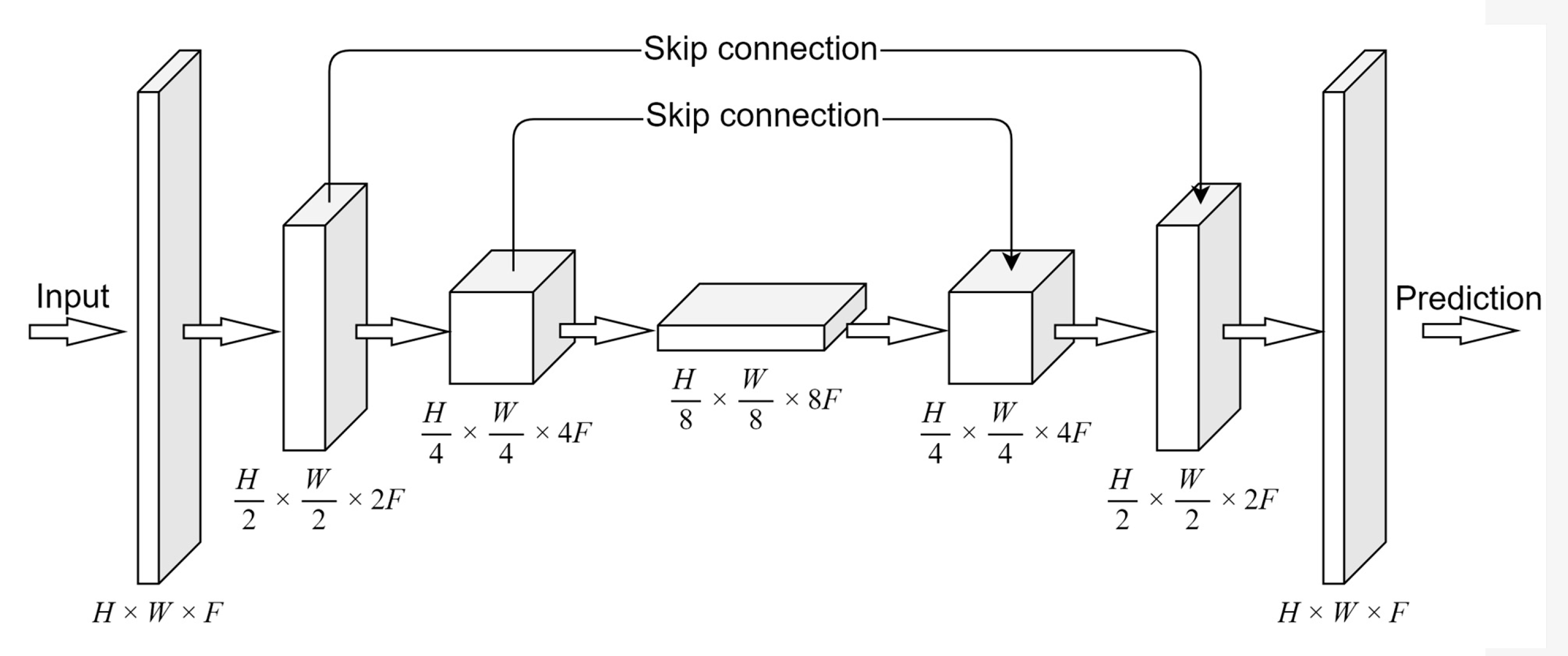
2.2. Deep Learning Models
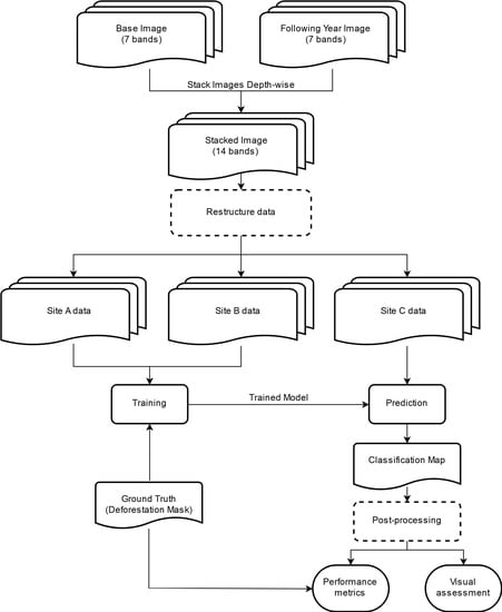
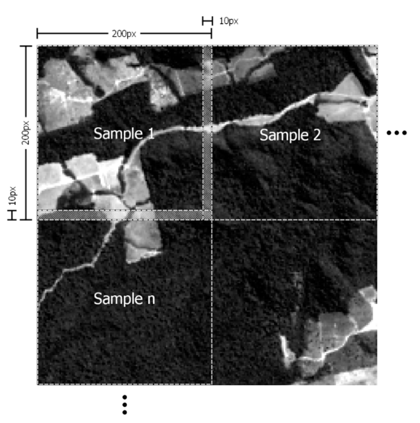
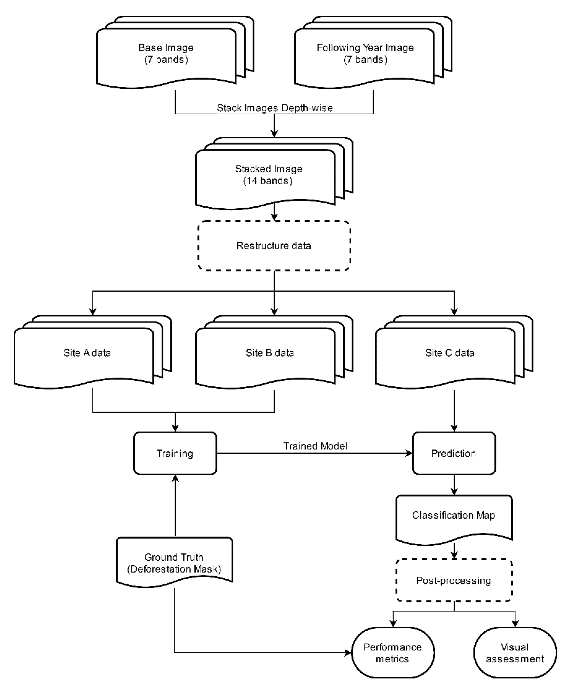
2.3. Data Structure
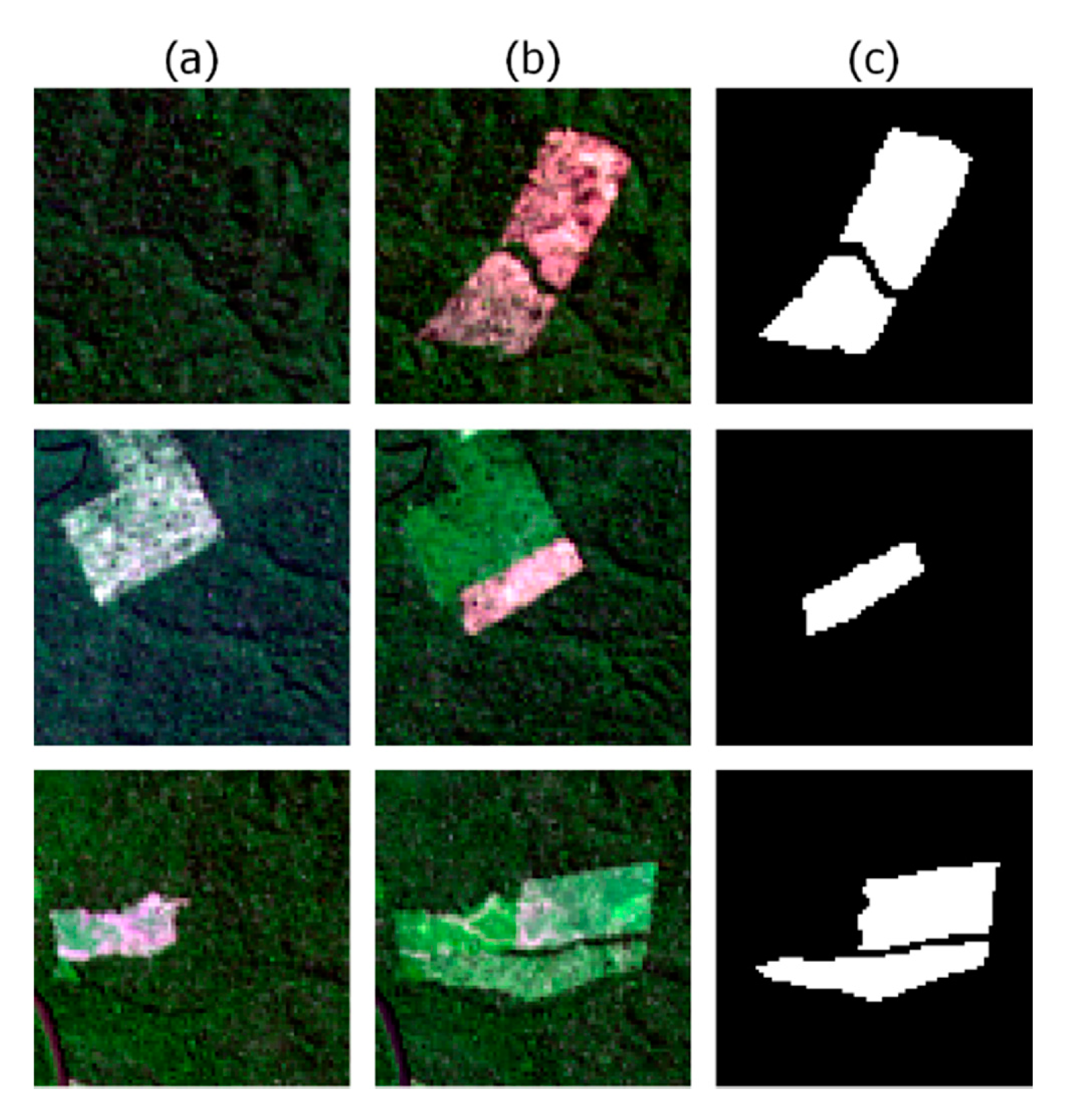
2.4. Ground Truth
2.5. Hyperparameters
2.6. Modeling Approach
2.7. Accuracy Assessment
3. Results
4. Discussion
5. Conclusions
Author Contributions
Funding
Acknowledgments
Conflicts of Interest
References
- Le Quéré, C.; Andrew, R.M.; Friedlingstein, P.; Sitch, S.; Hauck, J.; Pongratz, J.; Pickers, P.A.; Korsbakken, J.I.; Peters, G.P.; Canadell, J.G.; et al. Global carbon budget 2018. Earth Syst. Sci. Data 2018, 10, 2141–2194. [Google Scholar] [CrossRef]
- Aragão, L.E.O.C.; Poulter, B.; Barlow, J.B.; Anderson, L.O.; Malhi, Y.; Saatchi, S.; Phillips, O.L.; Gloor, E. Environmental change and the carbon balance of Amazonian forests: Environmental change in Amazonia. Biol. Rev. 2014, 89, 913–931. [Google Scholar] [CrossRef] [PubMed]
- Rosa, I.M.D.; Smith, M.J.; Wearn, O.R.; Purves, D.; Ewers, R.M. The environmental legacy of modern tropical deforestation. Curr. Biol. 2016, 26, 2161–2166. [Google Scholar] [CrossRef] [PubMed]
- Vedovato, L.B.; Fonseca, M.G.; Arai, E.; Anderson, L.O.; Aragão, L.E.O.C. The extent of 2014 forest fragmentation in the Brazilian Amazon. Reg. Environ. Chang. 2016, 16, 2485–2490. [Google Scholar] [CrossRef]
- Spracklen, D.V.; Garcia-Carreras, L. The impact of Amazonian deforestation on Amazon basin rainfall: Amazonian deforestation and rainfall. Geophys. Res. Lett. 2015, 42, 9546–9552. [Google Scholar] [CrossRef]
- Boisier, J.P.; Ciais, P.; Ducharne, A.; Guimberteau, M. Projected strengthening of Amazonian dry season by constrained climate model simulations. Nat. Clim. Chang. 2015, 5, 656–660. [Google Scholar] [CrossRef]
- INPE Projeto PRODES: Monitoramento da Floresta Amazônica Brasileira por satélite. Available online: http://www.obt.inpe.br/OBT/assuntos/programas/amazonia/prodes (accessed on 7 October 2019).
- INPE Projeto TerraClass. Available online: http://www.inpe.br/cra/projetos_pesquisas/dados_terraclass.php (accessed on 7 October 2019).
- Pearson, T.R.H.; Brown, S.; Murray, L.; Sidman, G. Greenhouse gas emissions from tropical forest degradation: An underestimated source. Carbon Balance Manag. 2017, 12, 3. [Google Scholar] [CrossRef]
- Singh, A. Review article digital change detection techniques using remotely-sensed data. Int. J. Remote Sens. 1989, 10, 989–1003. [Google Scholar] [CrossRef]
- Guo, E.; Fu, X.; Zhu, J.; Deng, M.; Liu, Y.; Zhu, Q.; Li, H. Learning to Measure Change: Fully Convolutional Siamese Metric Networks for Scene Change Detection. arXiv 2018, arXiv:1810.09111. [Google Scholar]
- Coppin, P.; Jonckheere, I.; Nackaerts, K.; Muys, B.; Lambin, E. Digital change detection methods in ecosystem monitoring: A review. Int. J. Remote Sens. 2004, 25, 1565–1596. [Google Scholar] [CrossRef]
- Lu, D.; Mausel, P.; Brondízio, E.; Moran, E. Change detection techniques. Int. J. Remote Sens. 2004, 25, 2365–2401. [Google Scholar] [CrossRef]
- Radke, R.J.; Andra, S.; Al-Kofahi, O.; Roysam, B. Image change detection algorithms: A systematic survey. IEEE Trans. Image Process. 2005, 14, 294–307. [Google Scholar] [CrossRef] [PubMed]
- Warner, T.; Almutairi, A.; Lee, J.Y. Remote sensing of land cover change. In The SAGE Handbook of Remote Sensing; Warner, T.A., Nellis, D.M., Foody, G.M., Eds.; SAGE Publications: London, UK, 2009; pp. 459–472. [Google Scholar]
- Hecheltjen, A.; Thonfeld, F.; Menz, G. Recent Advances in Remote Sensing Change Detection—A Review. In Land Use and Land Cover Mapping in Europe; Manakos, I., Braun, M., Eds.; Springer: Dordrecht, The Netherlands, 2014; Volume 18, pp. 145–178. [Google Scholar]
- Zhu, Z. Change detection using landsat time series: A review of frequencies, preprocessing, algorithms, and applications. ISPRS J. Photogramm. Remote Sens. 2017, 130, 370–384. [Google Scholar] [CrossRef]
- Tewkesbury, A.P.; Comber, A.J.; Tate, N.J.; Lamb, A.; Fisher, P.F. A critical synthesis of remotely sensed optical image change detection techniques. Remote Sens. Environ. 2015, 160, 1–14. [Google Scholar] [CrossRef]
- Ghosh, S.; Roy, M.; Ghosh, A. Semi-supervised change detection using modified self-organizing feature map neural network. Appl. Soft Comput. 2014, 15, 1–20. [Google Scholar] [CrossRef]
- Schneider, A. Monitoring land cover change in urban and peri-urban areas using dense time stacks of Landsat satellite data and a data mining approach. Remote Sens. Environ. 2012, 124, 689–704. [Google Scholar] [CrossRef]
- Zhang, L.; Zhang, L.; Du, B. Deep learning for remote sensing data: A technical tutorial on the state of the art. IEEE Geosci. Remote Sens. Mag. 2016, 4, 22–40. [Google Scholar] [CrossRef]
- Ma, L.; Liu, Y.; Zhang, X.; Ye, Y.; Yin, G.; Johnson, B.A. Deep learning in remote sensing applications: A meta-analysis and review. ISPRS J. Photogramm. Remote Sens. 2019, 152, 166–177. [Google Scholar] [CrossRef]
- Hughes, L.; Schmitt, M.; Zhu, X. Mining hard negative samples for SAR-optical image matching using generative adversarial networks. Remote Sens. 2018, 10, 1552. [Google Scholar] [CrossRef]
- Ma, W.; Zhang, J.; Wu, Y.; Jiao, L.; Zhu, H.; Zhao, W. A Novel Two-Step Registration Method for Remote Sensing Images Based on Deep and Local Features. IEEE Trans. Geosci. Remote Sens. 2019, 57, 4834–4843. [Google Scholar] [CrossRef]
- Merkle, N.; Auer, S.; Müller, R.; Reinartz, P. Exploring the potential of conditional adversarial networks for optical and SAR image matching. IEEE J. Sel. Top. Appl. Earth Obs. Remote Sens. 2018, 11, 1811–1820. [Google Scholar] [CrossRef]
- Wang, S.; Quan, D.; Liang, X.; Ning, M.; Guo, Y.; Jiao, L. A deep learning framework for remote sensing image registration. ISPRS J. Photogramm. Remote Sens. 2018, 145, 148–164. [Google Scholar] [CrossRef]
- Carranza-García, M.; García-Gutiérrez, J.; Riquelme, J. A Framework for Evaluating Land Use and Land Cover Classification Using Convolutional Neural Networks. Remote Sens. 2019, 11, 274. [Google Scholar] [CrossRef]
- Kussul, N.; Lavreniuk, M.; Skakun, S.; Shelestov, A. Deep Learning Classification of Land Cover and Crop Types Using Remote Sensing Data. IEEE Geosci. Remote Sens. Lett. 2017, 14, 778–782. [Google Scholar] [CrossRef]
- Li, M.; Wang, L.; Wang, J.; Li, X.; She, J. Comparison of land use classification based on convolutional neural network. J. Appl. Remote Sens. 2020, 14, 1. [Google Scholar] [CrossRef]
- Scott, G.J.; England, M.R.; Starms, W.A.; Marcum, R.A.; Davis, C.H. Training Deep Convolutional Neural Networks for Land–Cover Classification of High-Resolution Imagery. IEEE Geosci. Remote Sens. Lett. 2017, 14, 549–553. [Google Scholar] [CrossRef]
- Chen, F.; Ren, R.; Van de Voorde, T.; Xu, W.; Zhou, G.; Zhou, Y. Fast Automatic Airport Detection in Remote Sensing Images Using Convolutional Neural Networks. Remote Sens. 2018, 10, 443. [Google Scholar] [CrossRef]
- Kang, M.; Ji, K.; Leng, X.; Lin, Z. Contextual Region-Based Convolutional Neural Network with Multilayer Fusion for SAR Ship Detection. Remote Sens. 2017, 9, 860. [Google Scholar] [CrossRef]
- Qian, X.; Lin, S.; Cheng, G.; Yao, X.; Ren, H.; Wang, W. Object Detection in Remote Sensing Images Based on Improved Bounding Box Regression and Multi-Level Features Fusion. Remote Sens. 2020, 12, 143. [Google Scholar] [CrossRef]
- Yu, L.; Wang, Z.; Tian, S.; Ye, F.; Ding, J.; Kong, J. Convolutional Neural Networks for Water Body Extraction from Landsat Imagery. Int. J. Comput. Intell. Syst. 2017, 16, 1750001. [Google Scholar] [CrossRef]
- Liu, X.; Liu, Q.; Wang, Y. Remote sensing image fusion based on two-stream fusion network. Inf. Fusion 2020, 55, 1–15. [Google Scholar] [CrossRef]
- Liu, Y.; Chen, X.; Wang, Z.; Wang, Z.J.; Ward, R.K.; Wang, X. Deep learning for pixel-level image fusion: Recent advances and future prospects. Inf. Fusion 2018, 42, 158–173. [Google Scholar] [CrossRef]
- Scarpa, G.; Vitale, S.; Cozzolino, D. Target-Adaptive CNN-Based Pansharpening. IEEE Trans. Geosci. Remote Sens. 2018, 56, 1–15. [Google Scholar] [CrossRef]
- Yuan, Q.; Wei, Y.; Meng, X.; Shen, H.; Zhang, L. A Multiscale and Multidepth Convolutional Neural Network for Remote Sensing Imagery Pan-Sharpening. IEEE J. Sel. Top. Appl. Earth Obs. Remote Sens. 2018, 11, 978–989. [Google Scholar] [CrossRef]
- Kemker, R.; Salvaggio, C.; Kanan, C. Algorithms for semantic segmentation of multispectral remote sensing imagery using deep learning. ISPRS J. Photogramm. Remote Sens. 2018, 145, 60–77. [Google Scholar] [CrossRef]
- Malambo, L.; Popescu, S.; Ku, N.-W.; Rooney, W.; Zhou, T.; Moore, S. A Deep Learning Semantic Segmentation-Based Approach for Field-Level Sorghum Panicle Counting. Remote Sens. 2019, 11, 2939. [Google Scholar] [CrossRef]
- Xiao, X.; Zhou, Z.; Wang, B.; Li, L.; Miao, L. Ship Detection under Complex Backgrounds Based on Accurate Rotated Anchor Boxes from Paired Semantic Segmentation. Remote Sens. 2019, 11, 2506. [Google Scholar] [CrossRef]
- Zhuo, X.; Fraundorfer, F.; Kurz, F.; Reinartz, P. Optimization of openstreetmap building footprints based on semantic information of oblique UAV images. Remote Sens. 2018, 10, 624. [Google Scholar] [CrossRef]
- Xing, H.; Meng, Y.; Wang, Z.; Fan, K.; Hou, D. Exploring geo-tagged photos for land cover validation with deep learning. ISPRS J. Photogramm. Remote Sens. 2018, 141, 237–251. [Google Scholar] [CrossRef]
- Khan, S.H.; He, X.; Porikli, F.; Bennamoun, M. Forest change detection in incomplete satellite images with deep neural networks. IEEE Trans. Geosci. Remote Sens. 2017, 55, 5407–5423. [Google Scholar] [CrossRef]
- Mou, L.; Bruzzone, L.; Zhu, X.X. Learning Spectral-Spatial-Temporal Features via a Recurrent Convolutional Neural Network for Change Detection in Multispectral Imagery. IEEE Trans. Geosci. Remote Sens. 2018, 57, 924–935. [Google Scholar] [CrossRef]
- Ajami, A.; Ku er, M.; Persello, C.; Pfeffer, K. Identifying a slums’ degree of deprivation from VHR images using convolutional neural networks. Remote Sens. 2019, 11, 1282. [Google Scholar] [CrossRef]
- Cao, G.; Li, Y.; Liu, Y.; Shang, Y. Automatic change detection in high-resolution remote-sensing images by means of level set evolution and support vector machine classification. Int. J. Remote Sens. 2014, 35, 6255–6270. [Google Scholar] [CrossRef]
- Mboga, N.; Persello, C.; Bergado, J.R.; Stein, A. Detection of informal settlements from VHR images using convolutional neural networks. Remote Sens. 2017, 9, 1106. [Google Scholar] [CrossRef]
- Liu, R.; Kuffer, M.; Persello, C. The Temporal Dynamics of Slums Employing a CNN-Based Change Detection Approach. Remote Sens. 2019, 11, 2844. [Google Scholar] [CrossRef]
- Cao, C.; Dragićević, S.; Li, S. Land-use change detection with convolutional neural network methods. Environments 2019, 6, 25. [Google Scholar] [CrossRef]
- Zhang, X.; Shi, W.; Lv, Z.; Peng, F. Land cover change detection from high-resolution remote sensing imagery using multitemporal deep feature collaborative learning and a semi-supervised chan–vese model. Remote Sens. 2019, 11, 2787. [Google Scholar] [CrossRef]
- Zhang, C.; Sargent, I.; Pan, X.; Li, H.; Gardiner, A.; Hare, J.; Atkinson, P.M. An object-based convolutional neural network (OCNN) for urban land use classification. Remote Sens. Environ. 2018, 216, 57–70. [Google Scholar] [CrossRef]
- Liu, Y.; Wu, L. Geological disaster recognition on optical remote sensing images using deep learning. Procedia Comput. Sci. 2016, 91, 566–575. [Google Scholar] [CrossRef]
- Peng, D.; Zhang, Y.; Guan, H. End-to-End Change Detection for High Resolution Satellite Images Using Improved UNet++. Remote Sens. 2019, 11, 1382. [Google Scholar] [CrossRef]
- Hou, B.; Wang, Y.; Liu, Q. Change Detection Based on Deep Features and Low Rank. IEEE Geosci. Remote Sens. Lett. 2017, 14, 2418–2422. [Google Scholar] [CrossRef]
- Niu, X.; Gong, M.; Zhan, T.; Yang, Y. A Conditional Adversarial Network for Change Detection in Heterogeneous Images. IEEE Geosci. Remote Sens. Lett. 2019, 16, 45–49. [Google Scholar] [CrossRef]
- Zhang, M.; Xu, G.; Chen, K.; Yan, M.; Sun, X. Triplet-Based Semantic Relation Learning for Aerial Remote Sensing Image Change Detection. IEEE Geosci. Remote Sens. Lett. 2019, 16, 266–270. [Google Scholar] [CrossRef]
- Gong, M.; Zhan, T.; Zhang, P.; Miao, Q. Superpixel-based difference representation learning for change detection in multispectral remote sensing images. IEEE Trans. Geosci. Remote Sens. 2017, 55, 2658–2673. [Google Scholar] [CrossRef]
- Ma, W.; Xiong, Y.; Wu, Y.; Yang, H.; Zhang, X.; Jiao, L. Change Detection in Remote Sensing Images Based on Image Mapping and a Deep Capsule Network. Remote Sens. 2019, 11, 626. [Google Scholar] [CrossRef]
- Wang, Q.; Yuan, Z.; Du, Q.; Li, X. GETNET: A General End-to-End 2-D CNN Framework for Hyper- spectral Image Change Detection. IEEE Trans. Geosci. Remote Sens. 2018, 57, 3–13. [Google Scholar] [CrossRef]
- Zhang, W.; Lu, X. The Spectral-Spatial Joint Learning for Change Detection in Multispectral Imagery. Remote Sens. 2019, 11, 240. [Google Scholar] [CrossRef]
- Lebedev, M.; Vizilter, Y.V.; Vygolov, O.; Knyaz, V.; Rubis, A.Y. Change detection in remote sensing images using conditional adversarial networks. Int. Arch. Photogramm. Remote Sens. Spat. Inf. Sci. 2018, 42, 565–571. [Google Scholar] [CrossRef]
- Lei, T.; Zhang, Y.; Lv, Z.; Li, S.; Liu, S.; Nandi, A.K. Landslide Inventory Mapping from Bi-temporal Images Using Deep Convolutional Neural Networks. IEEE Geosci. Remote Sens. Lett. 2019, 16, 982–986. [Google Scholar] [CrossRef]
- Daudt, R.C.; Le Saux, B.; Boulch, A.; Gousseau, Y. High Resolution Semantic Change Detection. arXiv 2018, arXiv:1810.08452v1. [Google Scholar]
- Arima, E.Y.; Walker, R.T.; Perz, S.; Souza, C. Explaining the fragmentation in the Brazilian Amazonian forest. J. Land Use Sci. 2015, 1–21. [Google Scholar] [CrossRef]
- Godar, J.; Tizado, E.J.; Pokorny, B. Who is responsible for deforestation in the Amazon? A spatially explicit analysis along the Transamazon Highway in Brazil. Forest Ecol. Manag. 2012, 267, 58–73. [Google Scholar] [CrossRef]
- Carrero, G.C.; Fearnside, P.M. Forest clearing dynamics and the expansion of landholdings in Apuí, a deforestation hotspot on Brazil’s Transamazon Highway. Ecol. Soc. 2011, 16, 26. [Google Scholar] [CrossRef]
- Li, G.; Lu, D.; Moran, E.; Calvi, M.F.; Dutra, L.V.; Batistella, M. Examining deforestation and agropasture dynamics along the Brazilian TransAmazon Highway using multitemporal Landsat imagery. Gisci. Remote Sens. 2019, 56, 161–183. [Google Scholar] [CrossRef]
- Soares-Filho, B.; Alencar, A.; Nepstad, D.; Cerqueira, G.; Vera Diaz, M.D.C.; Rivero, S.; Solórzano, L.; Voll, E. Simulating the response of land-cover changes to road paving and governance along a major Amazon highway: The Santarem–Cuiaba corridor. Glob. Chang. Biol. 2004, 10, 745–764. [Google Scholar] [CrossRef]
- Müller, H.; Griffiths, P.; Hostert, P. Long-term deforestation dynamics in the Brazilian Amazon—Uncovering historic frontier development along the Cuiabá–Santarém highway. Int. J. Appl. Earth Obs. 2016, 44, 61–69. [Google Scholar] [CrossRef]
- Barber, C.P.; Cochrane, M.A.; Souza, C.M., Jr.; Laurance, W.F. Roads, deforestation, and the mitigating effect of protected areas in the Amazon. Biol. Conserv. 2014, 177, 203–209. [Google Scholar] [CrossRef]
- Fearnside, P.M. Highway construction as a force in destruction of the Amazon forest. In Handbook of Road Ecology; van der Ree, R., Smith, D.J., Grilo, C., Eds.; John Wiley & Sons Publishers: Oxford, UK, 2015; pp. 414–424. [Google Scholar]
- Alves, D.S. Space-time dynamics of deforestation in Brazilian Amazônia. Int. J. Remote Sens. 2002, 23, 2903–2908. [Google Scholar] [CrossRef]
- Arima, E.; Walker, R.T.; Perz, S.G.; Caldas, M. Loggers and forest fragmentation: Behavioral models of road building in the Amazon basin. Ann. Assoc. Am. Geogr. 2005, 95, 525–541. [Google Scholar] [CrossRef]
- Arima, E.Y.; Walker, R.T.; Sales, M.; Souza, C., Jr.; Perz, S.G. The fragmentation of space in the Amazon basin: Emergent road networks. Photogramm. Eng. Remote Sens. 2008, 74, 699–709. [Google Scholar] [CrossRef]
- Asner, G.P.; Broadbent, E.N.; Oliveira, P.J.C.; Keller, M.; Knapp, D.E.; Silva, J.N.M. Condition and fate of logged forests in the Brazilian Amazon. Proc. Natl. Acad. Sci. USA 2006, 103, 12947–12950. [Google Scholar] [CrossRef] [PubMed]
- Pfaff, A.; Robalino, J.; Walker, R.; Aldrich, S.; Caldas, M.; Reis, E.; Perz, S.; Bohrer, C.; Arima, E.; Laurance, W.; et al. Road investments, spatial spillovers, and deforestation in the Brazilian Amazon. J. Reg. Sci. 2007, 47, 109–123. [Google Scholar] [CrossRef]
- USGS. Landsat Collections: Landsat Collection 1. Available online: https://www.usgs.gov/land-resources/nli/landsat/landsat-collection-1 (accessed on 3 March 2020).
- Ronneberger, O.; Fischer, P.; Brox, T. U-Net: Convolutional Networks for Biomedical Image Segmentation. arXiv 2015, arXiv:1505.04597. [Google Scholar]
- Pinheiro, P.O.; Lin, T.-Y.; Collobert, R.; Dollàr, P. Learning to Refine Object Segments. arXiv 2016, arXiv:1603.08695. [Google Scholar]
- Zhang, Z.; Liu, Q.; Wang, Y. Road Extraction by Deep Residual U-Net. IEEE Geosci. Remote Sens. Lett. 2018, 15, 749–753. [Google Scholar] [CrossRef]
- Wei, S.; Zhang, H.; Wang, C.; Wang, Y.; Xu, L. Multi-Temporal SAR Data Large-Scale Crop Mapping Based on U-Net Model. Remote Sens. 2019, 11, 68. [Google Scholar] [CrossRef]
- Chollet, F. Keras. 2015. Available online: https://github.com/fchollet/keras (accessed on 3 March 2020).
- Abadi, M.; Agarwal, A.; Barham, P.; Brevdo, E.; Chen, Z.; Citro, C.; Corrado, G.S.; Davis, A.; Dean, J.; Devin, M.; et al. TensorFlow: Large-Scale Machine Learning on Heterogeneous Systems. arXiv 2016, arXiv:1603.04467. [Google Scholar]
- Shimabukuro, Y.E.; Arai, E.; Duarte, V.; Jorge, A.; Santos, E.G.; Gasparini, K.A.C.; Dutra, A.C. Monitoring deforestation and forest degradation using multi-temporal fraction images derived from Landsat sensor data in the Brazilian Amazon. Int. J. Remote Sens. 2019, 40, 5475–5496. [Google Scholar] [CrossRef]
- Cabral, A.I.R.; Saito, C.; Pereira, H.; Laques, A.E. Deforestation pattern dynamics in protected areas of the Brazilian Legal Amazon using remote sensing data. Appl. Geogr. 2018, 100, 101–115. [Google Scholar] [CrossRef]
- Quantum GIS Geographic Information System. Open Source Geospatial Foundation Project. Available online: http://www.qgis.org/it/site/ (accessed on 1 January 2020).
- Lin, T.-Y.; Goyal, P.; Girshick, R.; He, K.; Dollar, P. Focal Loss for Dense Object Detection. In Proceedings of the 2017 IEEE International Conference on Computer Vision (ICCV), Venice, Italy, 22–29 October 2017; pp. 2999–3007. [Google Scholar]
- Kingma, D.P.; Ba, J. Adam: A Method for Stochastic Optimization. arXiv 2014, arXiv:1412.6980. [Google Scholar]
- Belgiu, M.; Drăguţ, L. Random forest in remote sensing: A review of applications and future directions. ISPRS J. Photogramm. Remote Sens. 2016, 114, 24–31. [Google Scholar] [CrossRef]
- Mahmon, N.A.; Ya’acob, N. A review on classification of satellite image using Artificial Neural Network (ANN). In Proceedings of the 2014 IEEE 5th Control and System Graduate Research Colloquium, Shah Alam, Malaysia, 11–12 August 2014; pp. 153–157. [Google Scholar]
- Stehman, S.V. Sampling designs for accuracy assessment of land cover. Int. J. Remote Sens. 2009, 30, 5243–5272. [Google Scholar] [CrossRef]
- Foody, G.M. Status of land cover classification accuracy assessment. Remote Sens. Environ. 2002, 80, 185–201. [Google Scholar] [CrossRef]
- Stehman, S. Comparing estimators of gross change derived from complete coverage mapping versus statistical sampling of remotely sensed data. Remote Sens. Environ. 2005, 96, 466–474. [Google Scholar] [CrossRef]
- McNemar, Q. Note on the sampling error of the difference between correlated proportions or percentages. Psychometrika 1947, 12, 153–157. [Google Scholar] [CrossRef]
- Liu, T.; Abd-Elrahman, A.; Morton, J.; Wilhelm, V.L. Comparing fully convolutional networks, random forest, support vector machine, and patch-based deep convolutional neural networks for object-based wetland mapping using images from small unmanned aircraft system. Gisci. Remote Sens. 2018, 55, 243–264. [Google Scholar] [CrossRef]
- Rakshit, S.; Debnath, S.; Mondal, D. Identifying Land Patterns from Satellite Imagery in Amazon Rainforest using Deep Learning. arXiv 2018, arXiv:1809.00340. [Google Scholar]
- Helber, P.; Bischke, B.; Dengel, A.; Borth, D. EuroSAT: A Novel Dataset and Deep Learning Benchmark for Land Use and Land Cover Classification. arXiv 2019, arXiv:1709.00029. [Google Scholar] [CrossRef]
- Ortega, M.X.; Bermudez, J.D.; Happ, P.N.; Gomes, A.; Feitosa, R.Q. Evaluation of Deep Learning Techniques for Deforestation Detection the Amazon Forest. ISPRS Ann. Photogramm. Remote Sens. Spatial Inf. Sci. 2019, IV-2/W7, 121–128. [Google Scholar] [CrossRef]
- Liu, C.-C.; Zhang, Y.-C.; Chen, P.-Y.; Lai, C.-C.; Chen, Y.-H.; Cheng, J.-H.; Ko, M.-H. Clouds Classification from Sentinel-2 Imagery with Deep Residual Learning and Semantic Image Segmentation. Remote Sens. 2019, 11, 119. [Google Scholar] [CrossRef]
- Li, L.; Liang, J.; Weng, M.; Zhu, H. A Multiple-Feature Reuse Network to Extract Buildings from Remote Sensing Imagery. Remote Sens. 2018, 10, 1350. [Google Scholar] [CrossRef]
- Ghorbanzadeh, O.; Blaschke, T.; Gholamnia, K.; Meena, S.; Tiede, D.; Aryal, J. Evaluation of Different Machine Learning Methods and Deep-Learning Convolutional Neural Networks for Landslide Detection. Remote Sens. 2019, 11, 196. [Google Scholar] [CrossRef]


| Site | Landsat Scene | Acquisition Date | ||
|---|---|---|---|---|
| 2017 | 2018 | 2019 | ||
| A | 227_63 | July 18 | July 21 | July 24 |
| B | 227_65 | July 18 | July 21 | July 24 |
| C | 230_65 | June 21 | June 24 | July 13 |
| Architecture | Layers | Parameters |
|---|---|---|
| U-Net | 69 | 1,933,866 |
| SharpMask | 114 | 221,386 |
| ResUnet | 93 | 2,068,554 |
| Model | 2017–2018 | 2017–2019 | ||||||||||
|---|---|---|---|---|---|---|---|---|---|---|---|---|
| F1 | Kappa | mIoU | Precision | Recall | Overall Accuracy | F1 | Kappa | mIoU | Precision | Recall | Overall Accuracy | |
| RF | 0.8014 | 0.8003 | 0.8332 | 0.9414 | 0.6976 | 0.9979 | 0.8902 | 0.8892 | 0.9000 | 0.8877 | 0.8928 | 0.9979 |
| MLP | 0.8926 | 0.8920 | 0.9024 | 0.9282 | 0.8597 | 0.9987 | 0.9101 | 0.9093 | 0.9167 | 0.9314 | 0.8898 | 0.9983 |
| Resunet | 0.9432 | 0.9428 | 0.9459 | 0.9252 | 0.9619 | 0.9993 | 0.9465 | 0.9460 | 0.9487 | 0.9358 | 0.9574 | 0.9990 |
| Unet | 0.9112 | 0.9106 | 0.9179 | 0.9223 | 0.9003 | 0.9989 | 0.9339 | 0.9332 | 0.9373 | 0.9175 | 0.9508 | 0.9987 |
| Sharpmask | 0.9223 | 0.9218 | 0.9274 | 0.9173 | 0.9274 | 0.9990 | 0.9337 | 0.9331 | 0.9372 | 0.9218 | 0.9460 | 0.9987 |
| 2017–2018 | 2018–2019 | |||||||||
|---|---|---|---|---|---|---|---|---|---|---|
| MLP | ResUnet | RF | SharpMask | U-Net | MLP | ResUnet | RF | SharpMask | U-Net | |
| MLP | ||||||||||
| ResUnet | <0.001 | <0.001 | ||||||||
| RF | <0.001 | <0.001 | <0.001 | <0.001 | ||||||
| SharpMask | <0.001 | <0.001 | <0.001 | <0.001 | <0.001 | <0.001 | ||||
| U-Net | <0.001 | <0.001 | <0.001 | <0.001 | <0.001 | <0.001 | <0.001 | <0.001 | ||
| Reference | Deforested Area (km2) | Difference from Ground Truth (%) | ||
|---|---|---|---|---|
| 2017–2018 | 2018–2019 | 2017–2018 | 2018–2019 | |
| Ground Truth | 152.73 | 233.44 | --- | --- |
| Random Forest | 113.17 | 234.79 | −25.90 | +0.58 |
| MultiLayer Perceptron | 141.45 | 223.01 | −7.39 | -4.47 |
| SharpMask | 154.40 | 239.56 | +1.10 | +2.62 |
| U-Net | 149.10 | 241.90 | −2.38 | +3.62 |
| ResUnet | 158.78 | 238.84 | +3.96 | +2.31 |
© 2020 by the authors. Licensee MDPI, Basel, Switzerland. This article is an open access article distributed under the terms and conditions of the Creative Commons Attribution (CC BY) license (http://creativecommons.org/licenses/by/4.0/).
Share and Cite
de Bem, P.P.; de Carvalho Junior, O.A.; Fontes Guimarães, R.; Trancoso Gomes, R.A. Change Detection of Deforestation in the Brazilian Amazon Using Landsat Data and Convolutional Neural Networks. Remote Sens. 2020, 12, 901. https://doi.org/10.3390/rs12060901
de Bem PP, de Carvalho Junior OA, Fontes Guimarães R, Trancoso Gomes RA. Change Detection of Deforestation in the Brazilian Amazon Using Landsat Data and Convolutional Neural Networks. Remote Sensing. 2020; 12(6):901. https://doi.org/10.3390/rs12060901
Chicago/Turabian Stylede Bem, Pablo Pozzobon, Osmar Abílio de Carvalho Junior, Renato Fontes Guimarães, and Roberto Arnaldo Trancoso Gomes. 2020. "Change Detection of Deforestation in the Brazilian Amazon Using Landsat Data and Convolutional Neural Networks" Remote Sensing 12, no. 6: 901. https://doi.org/10.3390/rs12060901
APA Stylede Bem, P. P., de Carvalho Junior, O. A., Fontes Guimarães, R., & Trancoso Gomes, R. A. (2020). Change Detection of Deforestation in the Brazilian Amazon Using Landsat Data and Convolutional Neural Networks. Remote Sensing, 12(6), 901. https://doi.org/10.3390/rs12060901