Evaluation of Deep Learning Techniques for Deforestation Detection in the Brazilian Amazon and Cerrado Biomes From Remote Sensing Imagery

 ,
,  , ,
, ,  and
and
Abstract
1. Introduction
Goals And Contributions
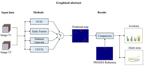
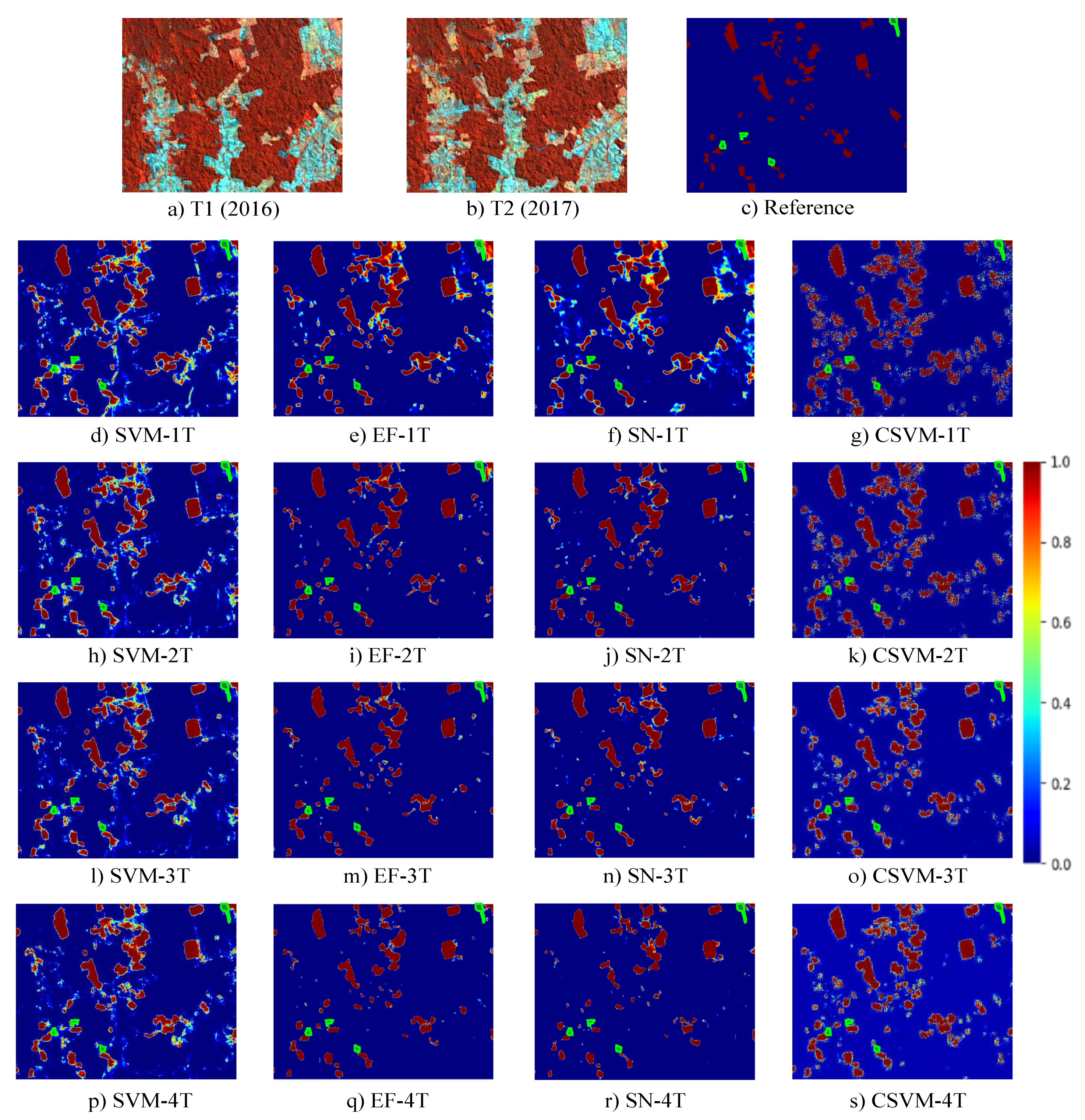
- An evaluation and comparison of three Deep Learning techniques for automatic deforestation detection in Brazilian Amazon and Cerrado biomes; namely, Early Fusion (EF), Siamese Network (SN), and Convolutional SVM (CSVM).
- An assessment of these methods’ accuracy under scarce training samples.
- An estimation for each method of the relation: area assigned as deforestation vs. area of true deforestation.
2. Materials and Methods
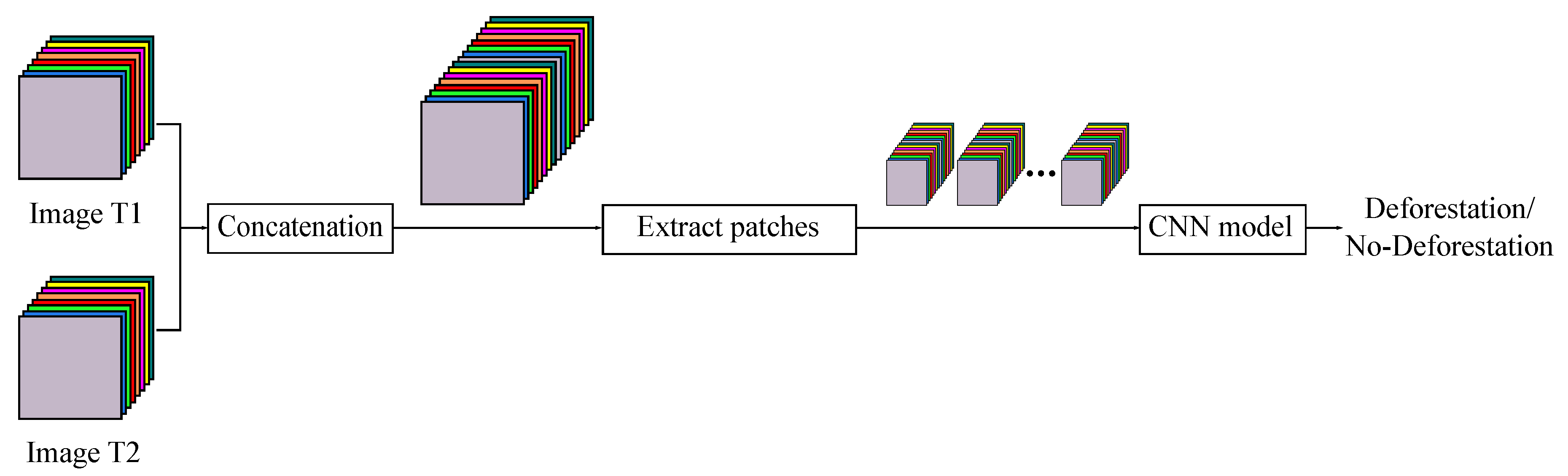
2.1. Early Fusion (EF)
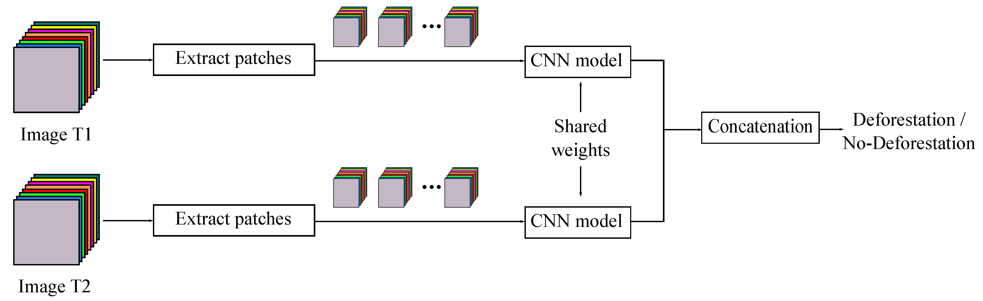
2.2. Siamese Network (SN)
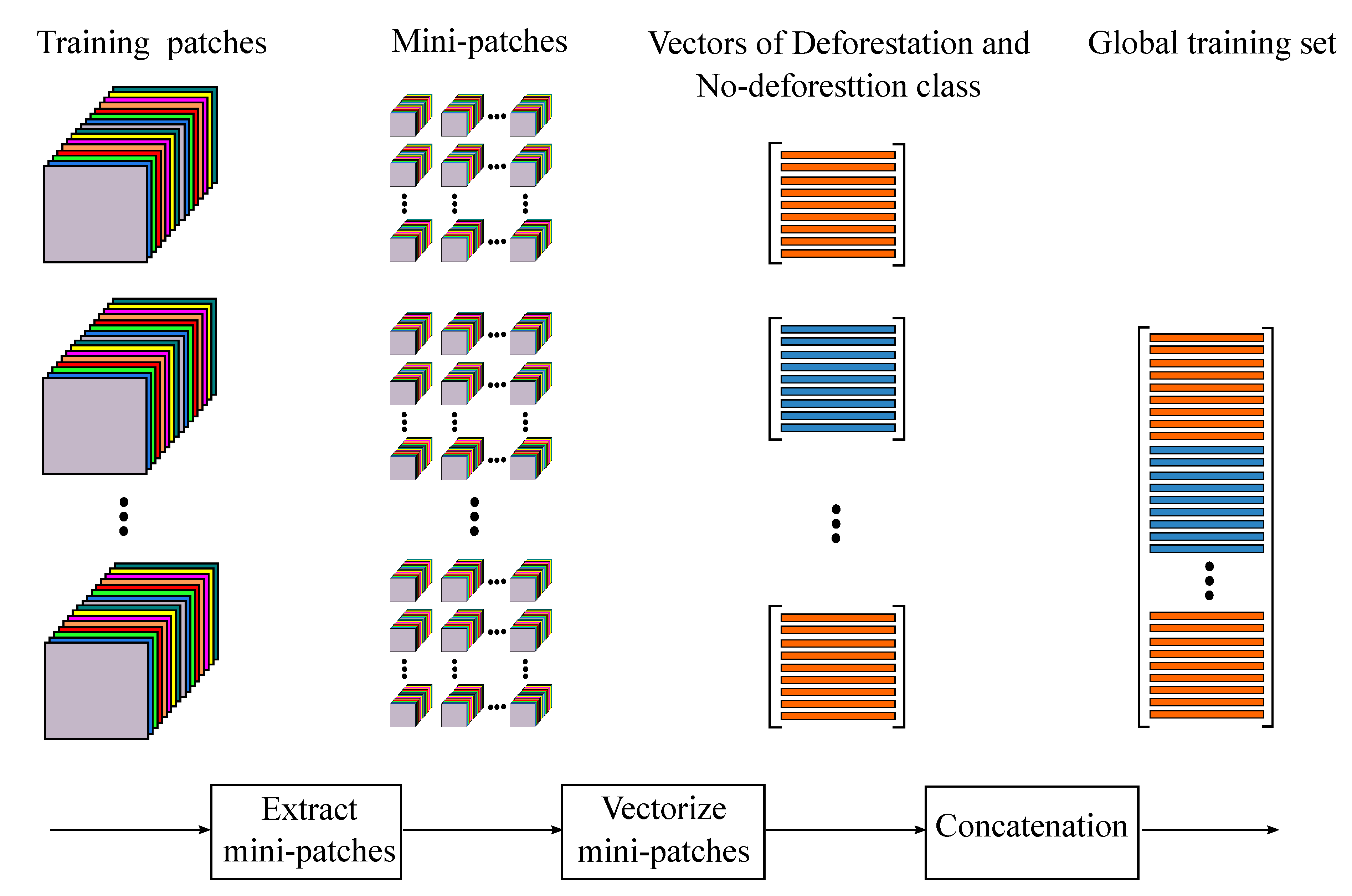
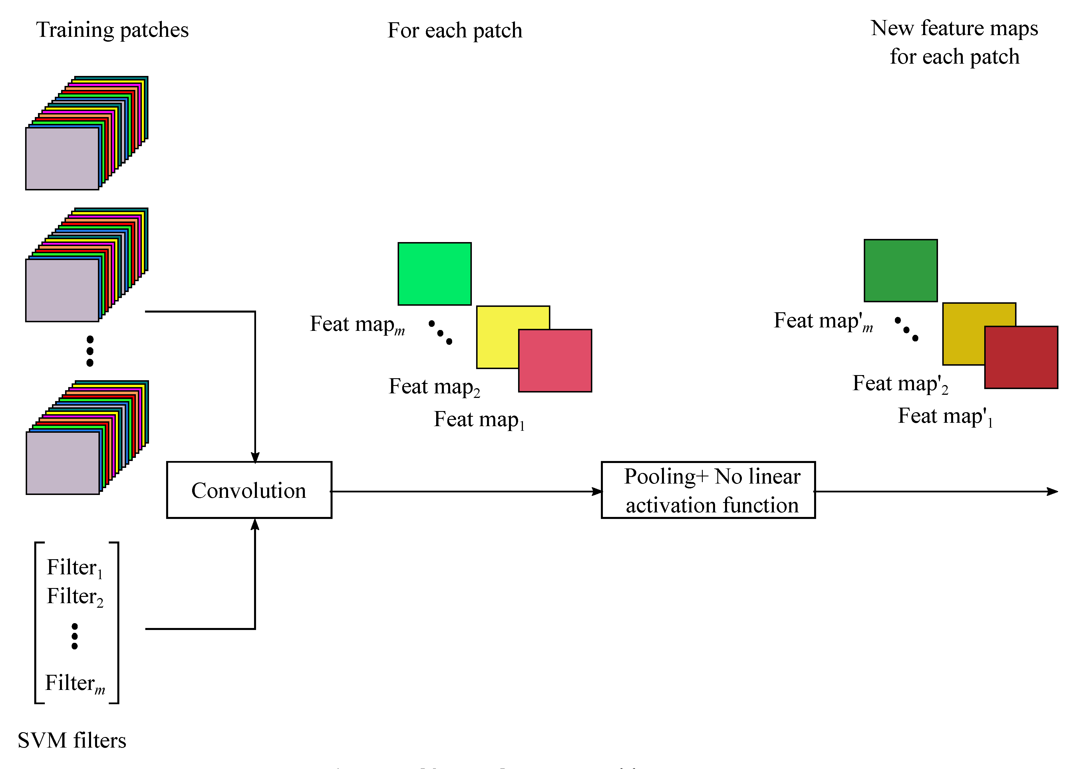
2.3. Convolutional SVM (CSVM)
2.3.1. Construction of Training Set
2.3.2. Training the SVMs Filter Bank
2.3.3. Generation of Feature Maps
2.3.4. Classification
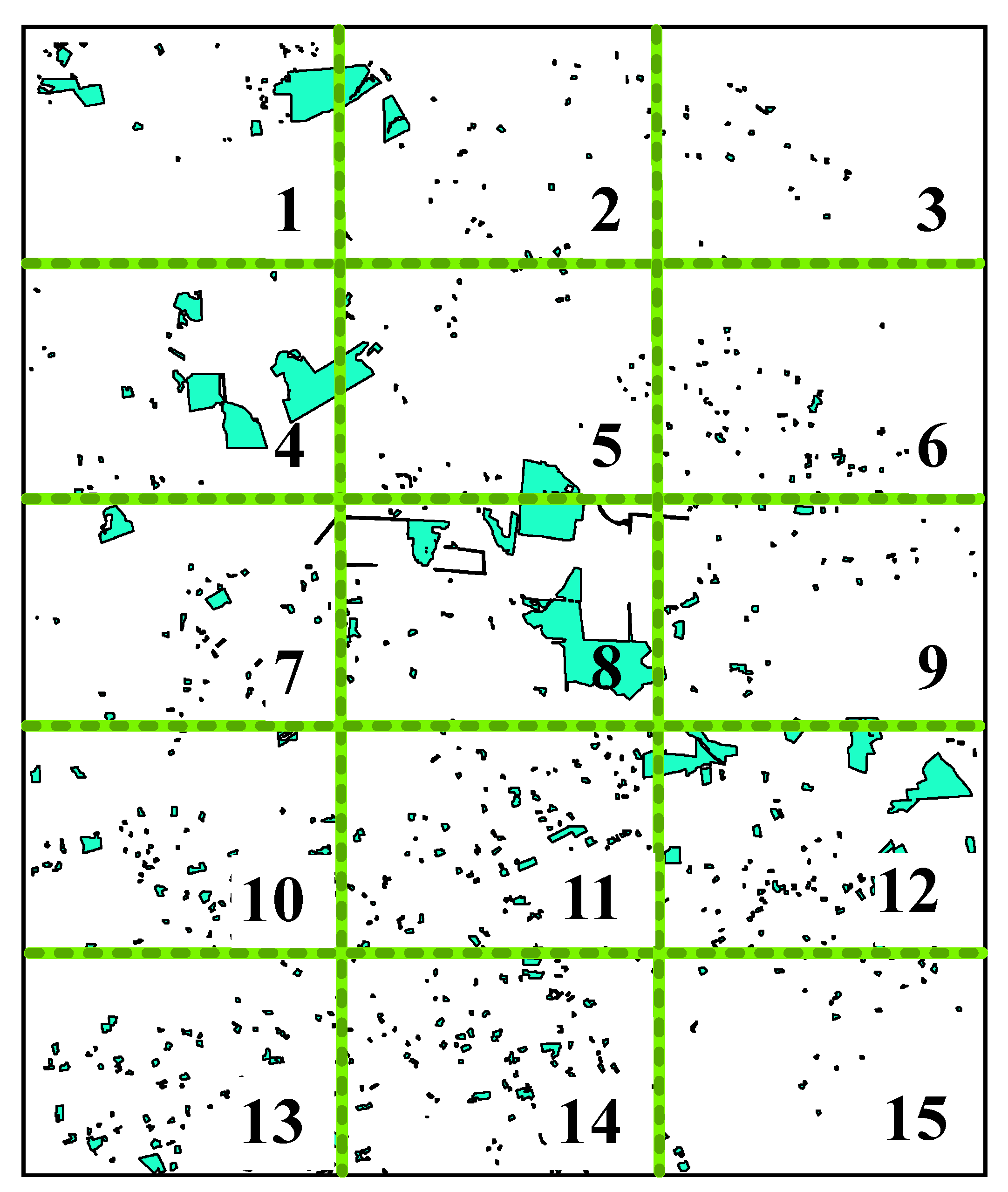
2.4. Study Areas
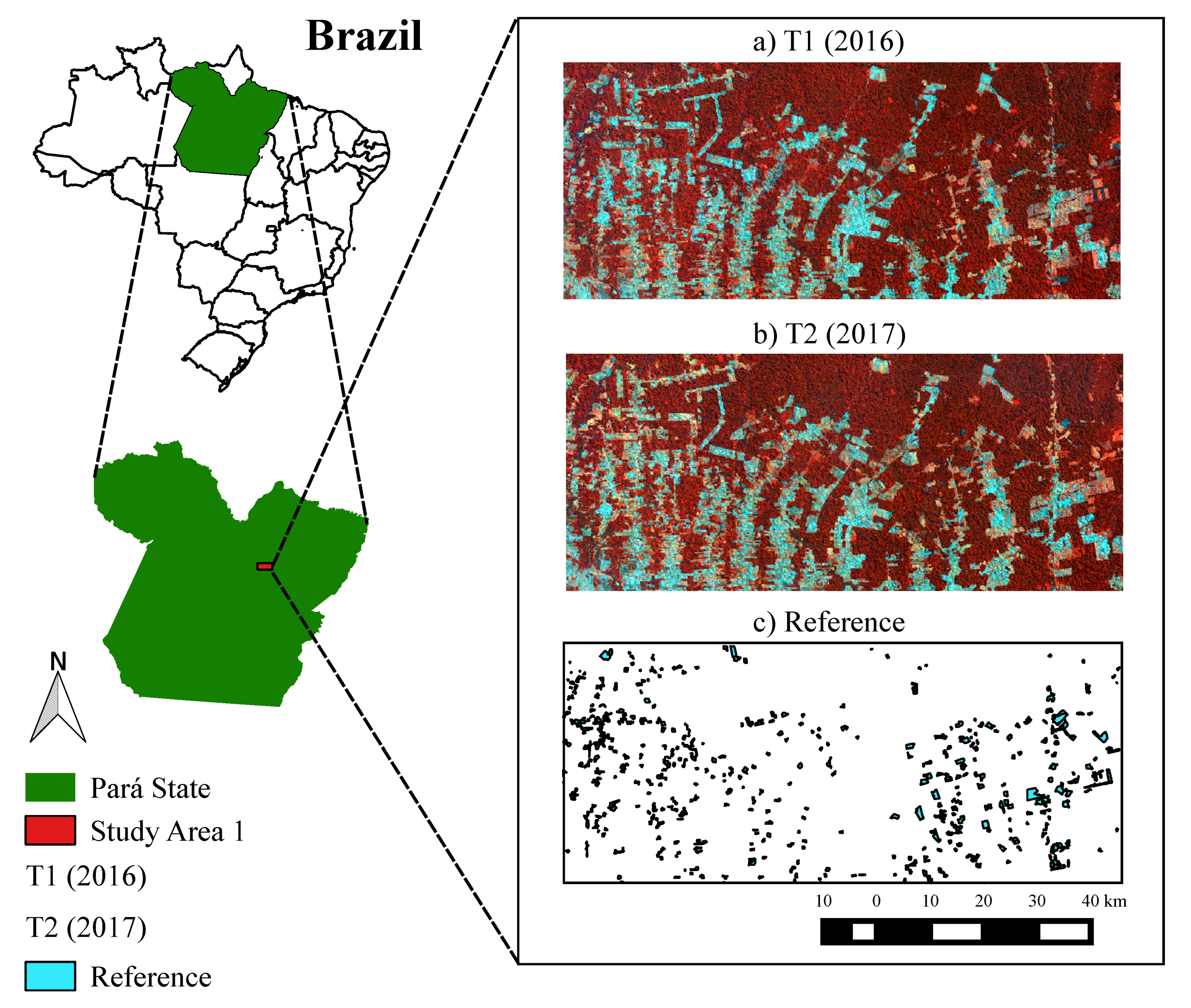
2.4.1. Amazon Biome
- Polygons of areas deforested in previous years (before August 2016) were disregarded.
- An external buffer of two pixels inside the polygons of class “deforestation” was not considered for the training, validation, and test. The reason was to avoid the impact of the variation between the photointerpreters estimation.
- Areas lower than 6.25 ha (69 pixels) were also not considered in our evaluation because PRODES data does not record deforestation areas smaller than that for the Amazon biome.
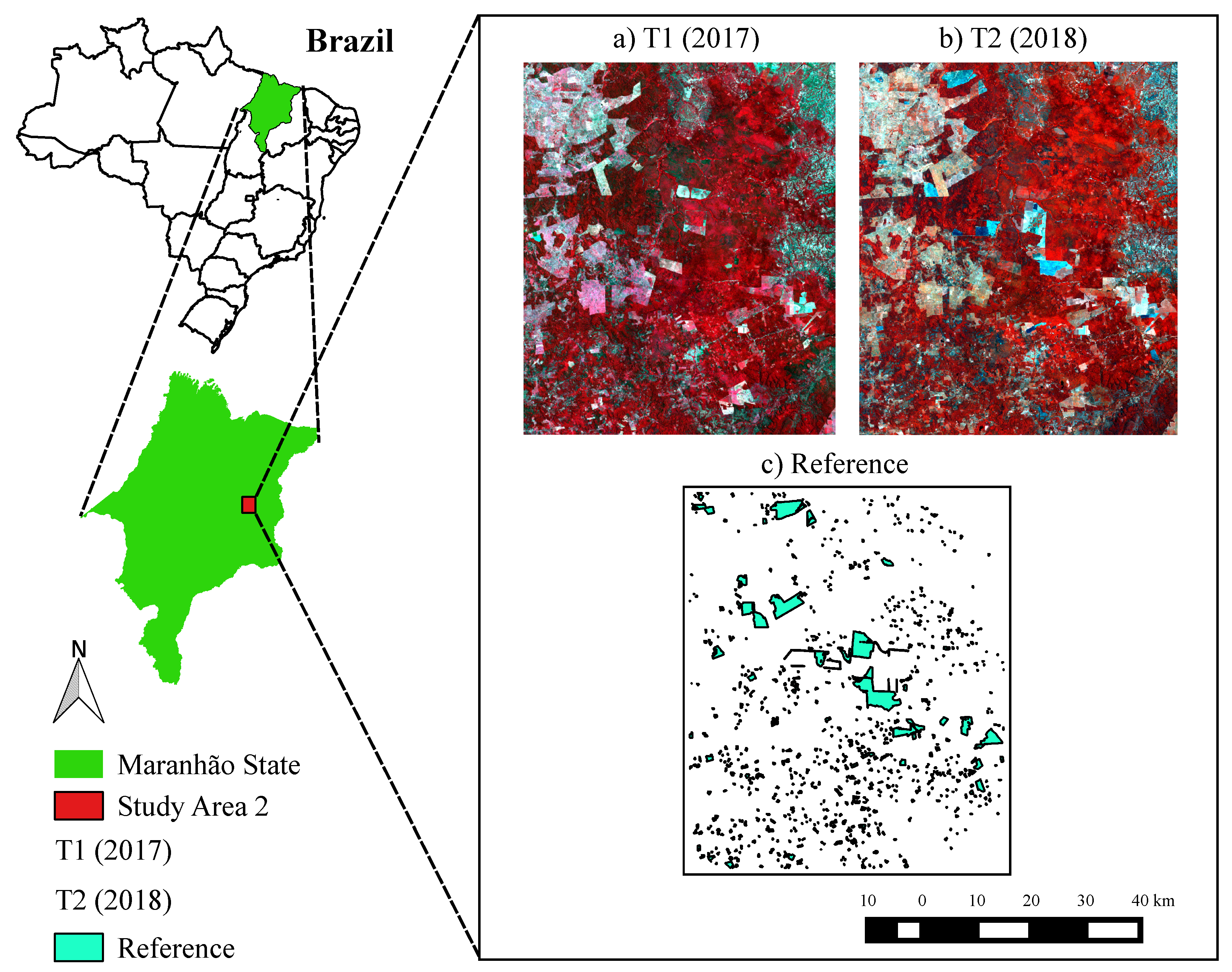
2.4.2. Cerrado Biome
- Some areas that suffered deforestation after the PRODES report were included in the reference. The added polygons were reviewed and approved by an expert photointerpreter. The final reference change map of the Cerrado is presented in Figure 6.
- An external buffer of two pixels around the samples of class “deforestation” was not considered in our evaluation to avoid the aforesaid inaccuracy problem along the borders.
- Areas lower than 1 ha (11 pixels) were not considered in the computation of the accuracy metrics because PRODES data does not consider deforested areas smaller than this value for the Cerrado biome.
2.5. Experimental Setup
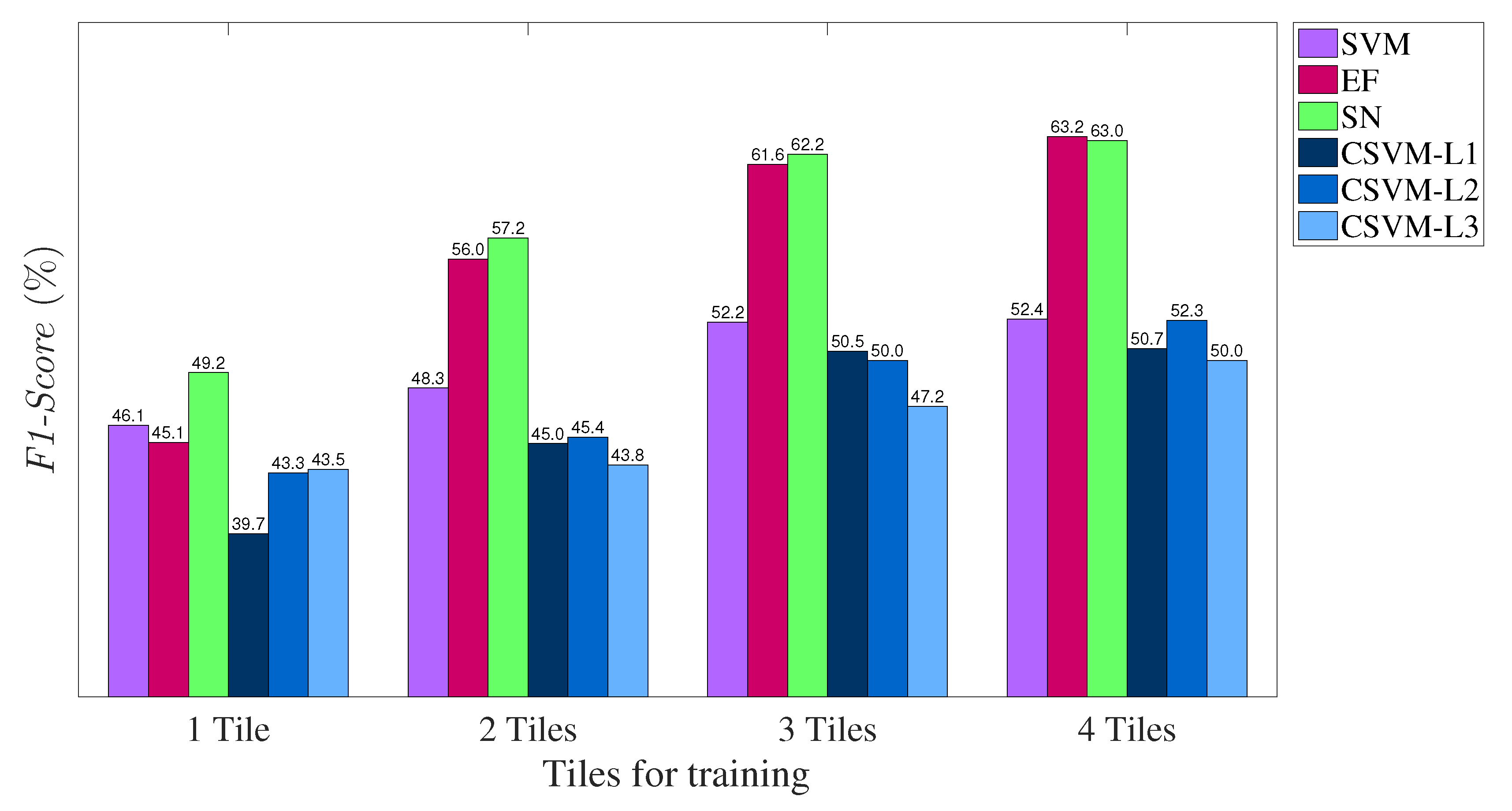
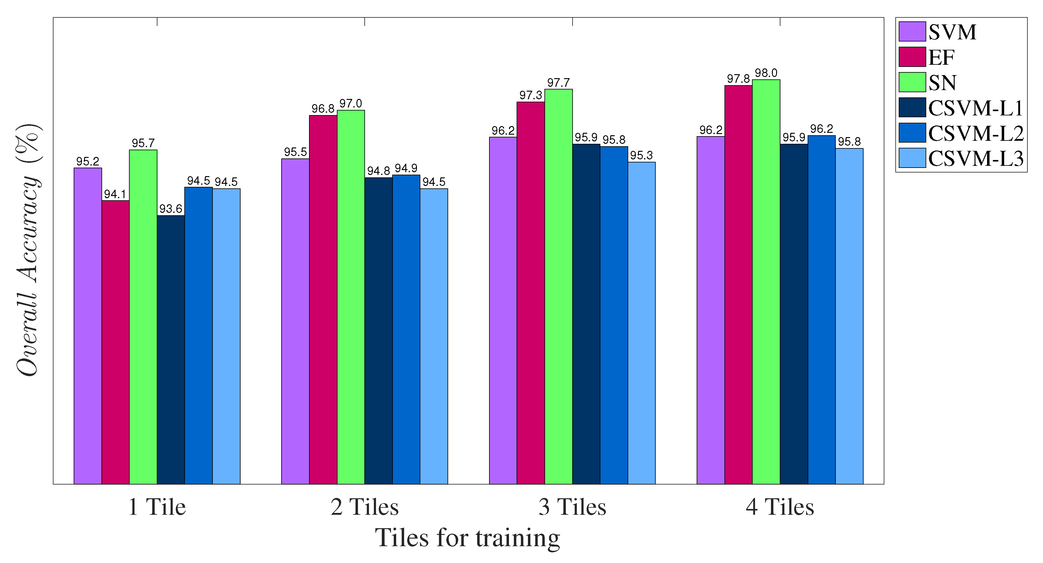
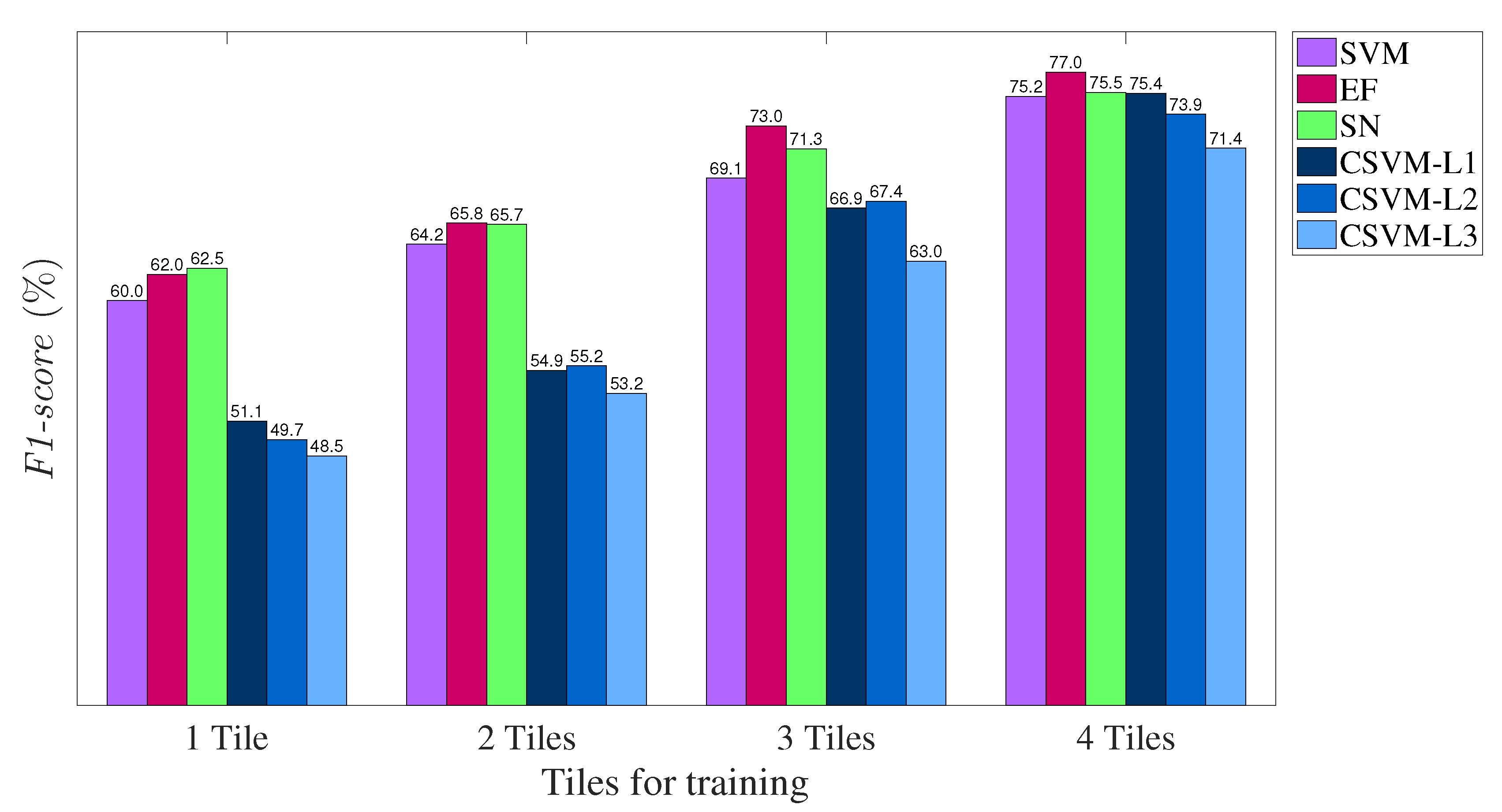
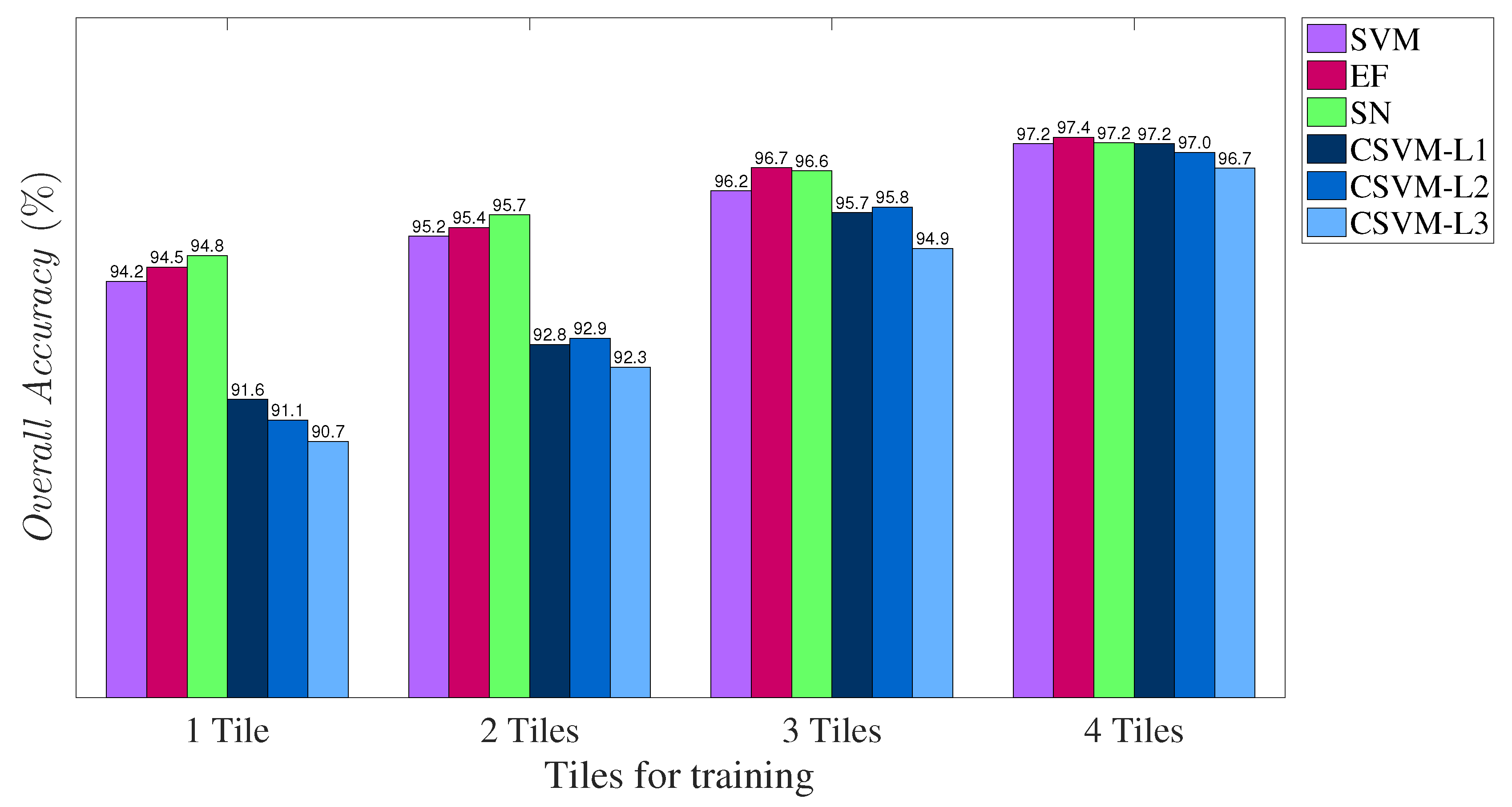
2.6. Influence of the Number of Training Samples
2.7. Accuracy Assessment
- Overall Accuracy (): is a global metric that indicates the percentage of samples correctly classified in relation to the total samples. It is defined by:where true positives () is the number of samples correctly assigned to the class “deforestation”, false positives () refer to the number of samples erroneously assigned to the class “deforestation”. Analogously, true negatives () and false negatives () correspond to the number of samples correctly and incorrectly assigned to the class “no-deforestation”, respectively. P and N denote the total number of positive and negative samples in the test set.
- Precision, also known as Correctness, represents the proportion of samples assigned by the classifier to the class “deforestation”, which truly belongs to that class, formally
- Recall, also known as Completeness, is the proportion of all “non deforestation” samples recognized by the classifier as such, i.e.,
- F1-score: is given by the harmonic mean of Precision and Recall and it also varies in a range of 0 to 1. This metric is defined by:
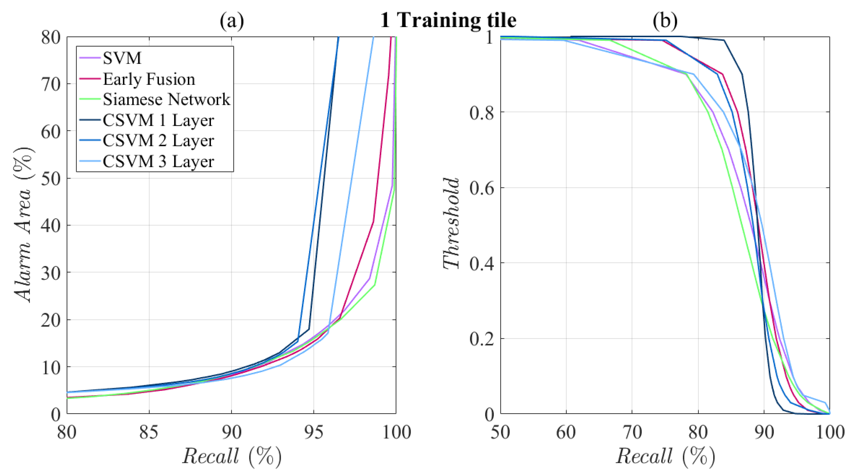
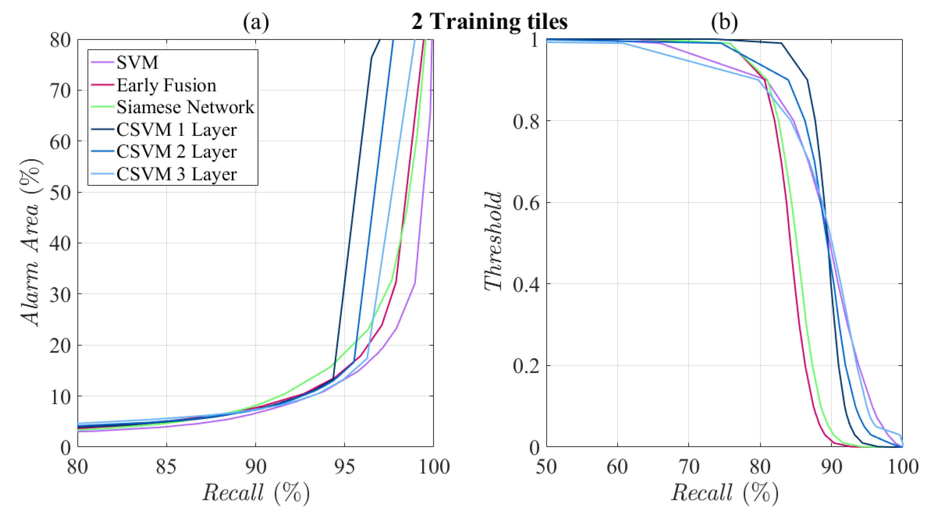
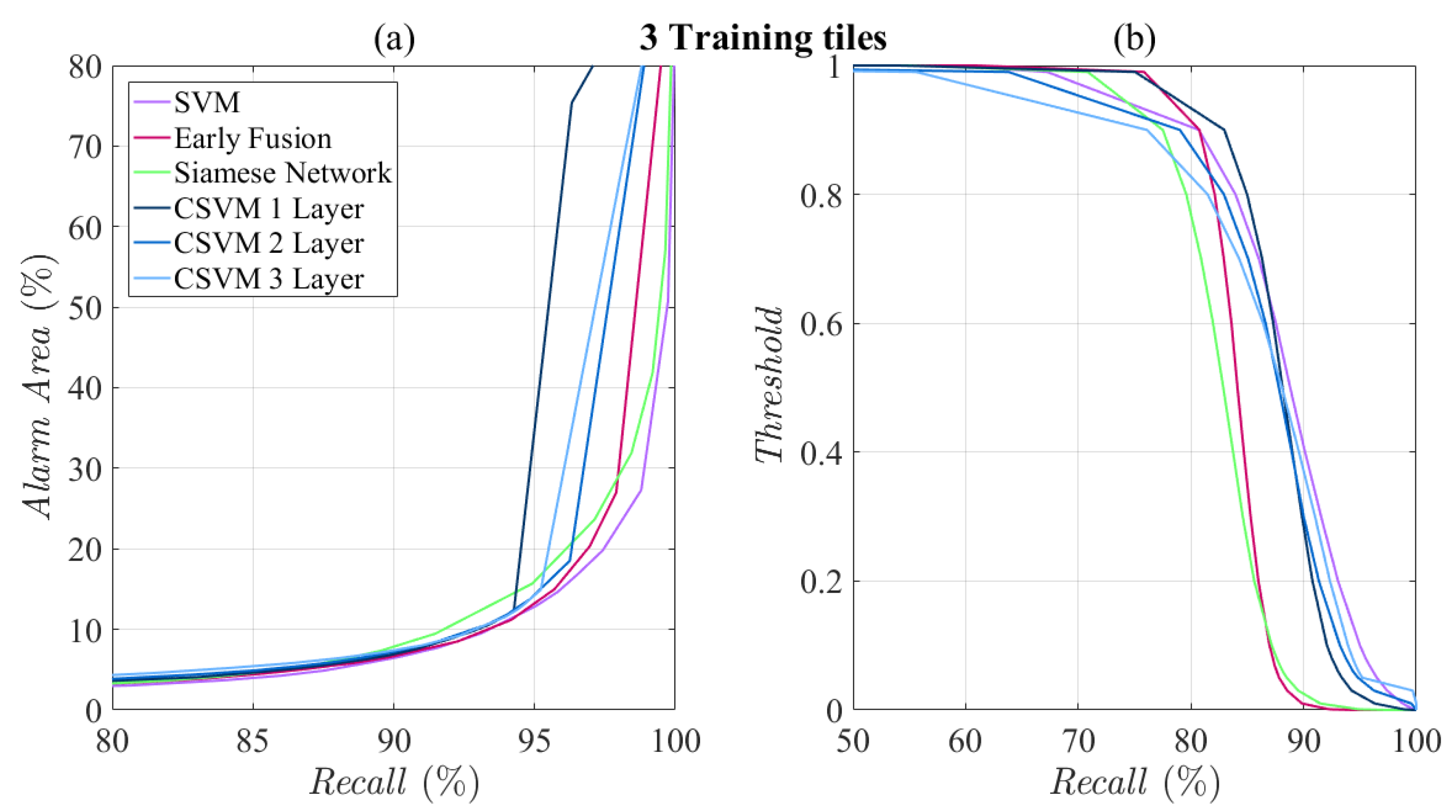
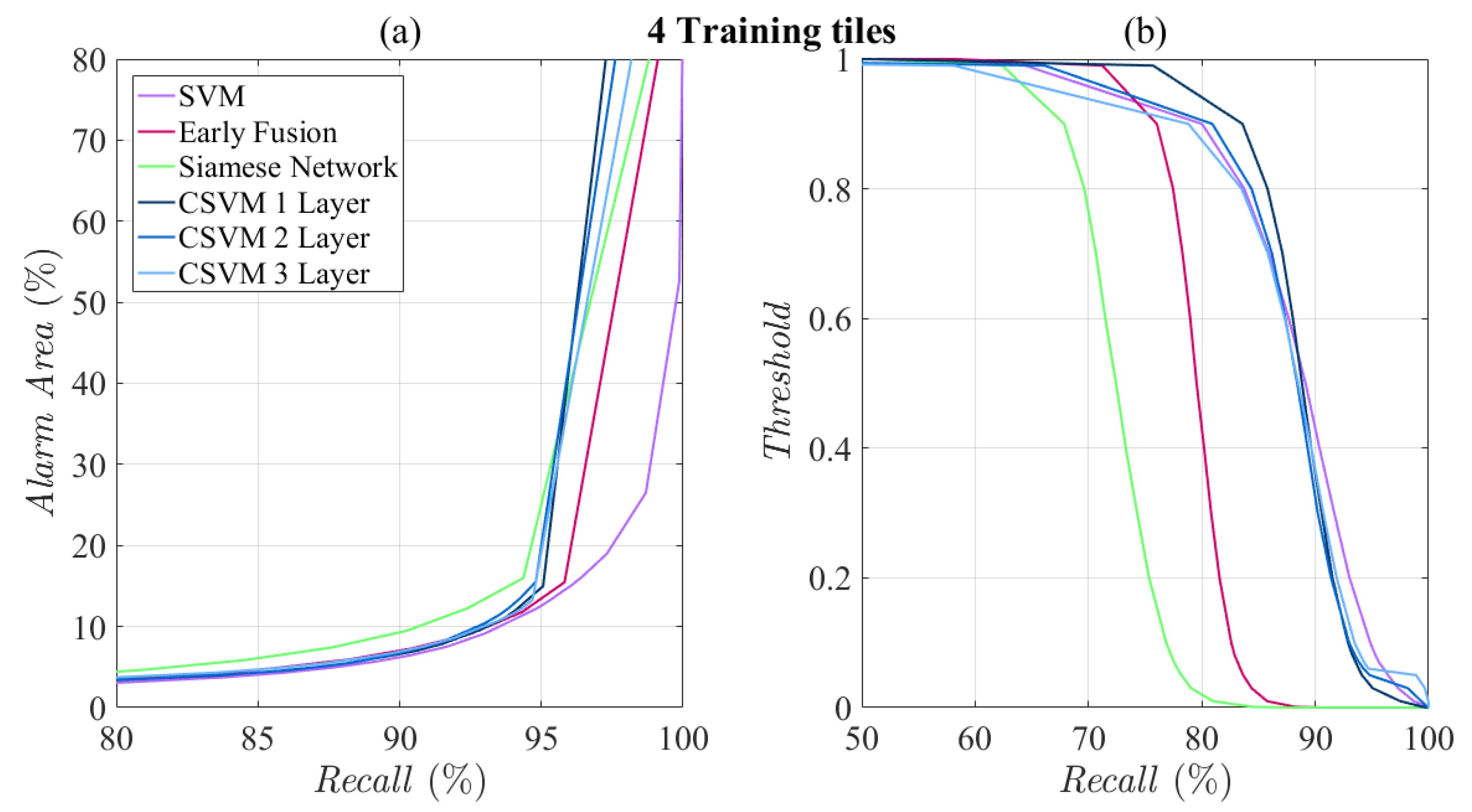
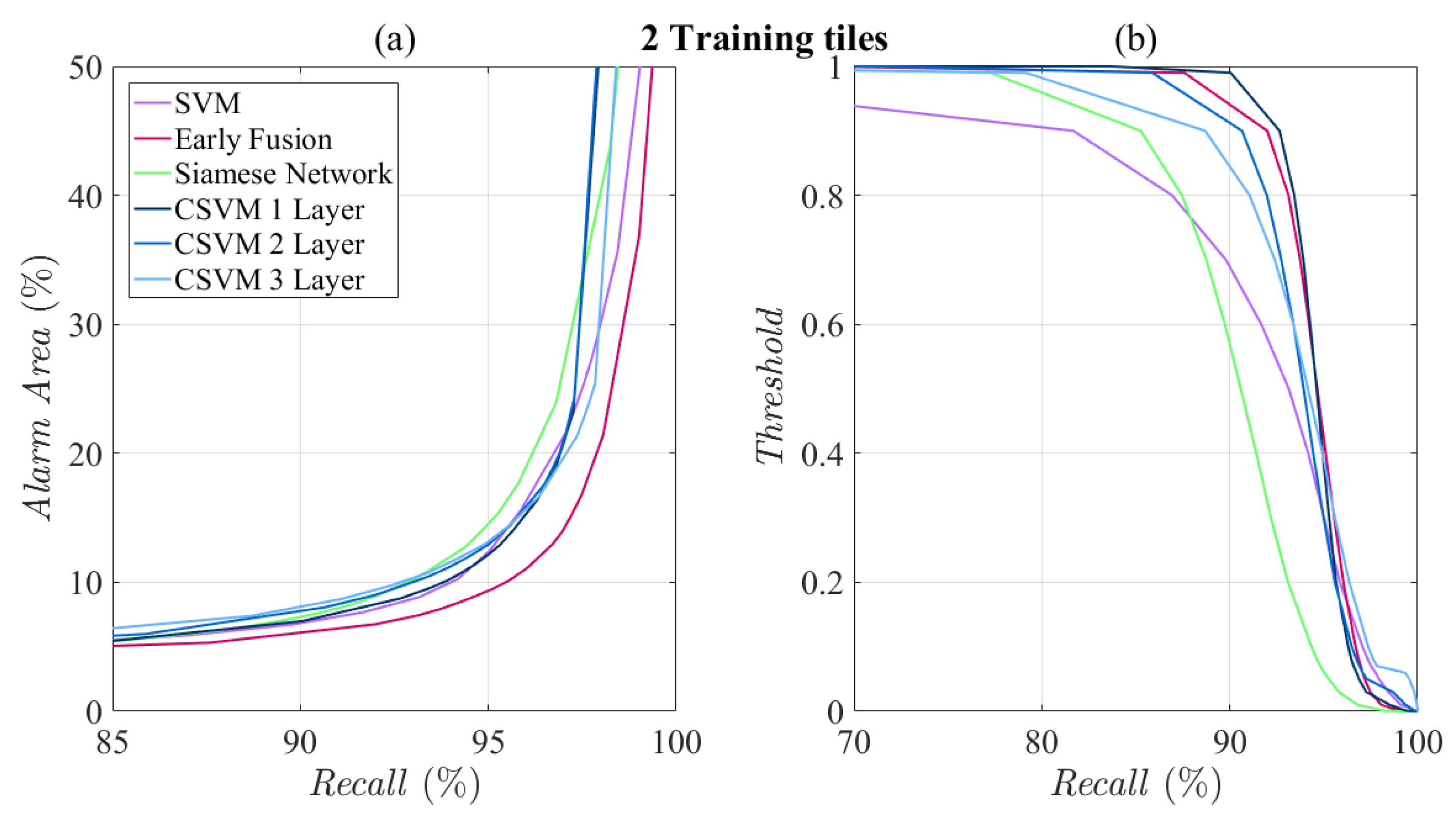
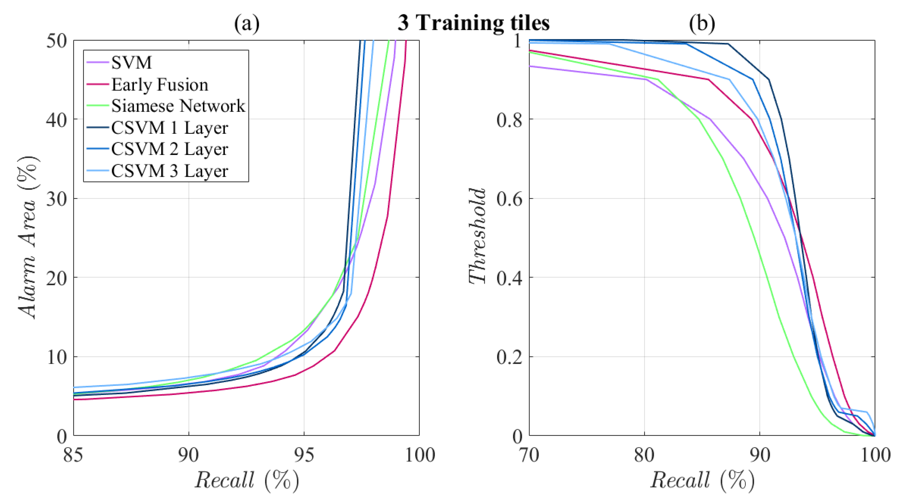
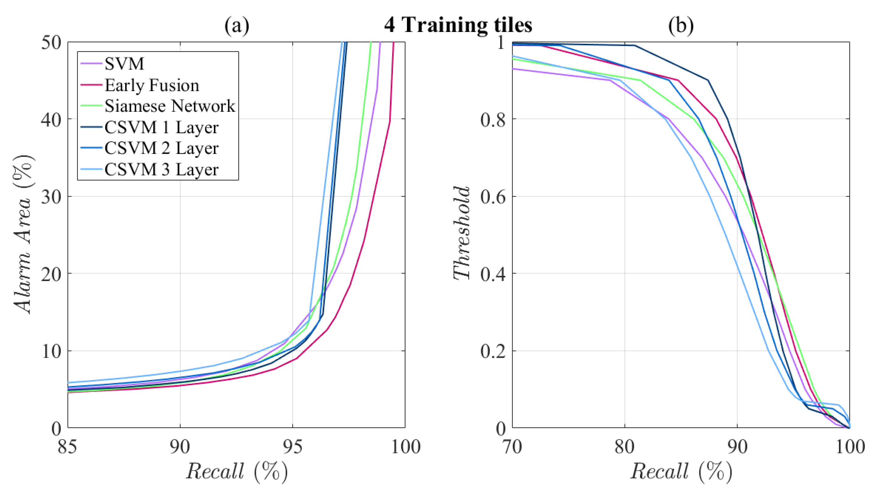
- Alarm Area: this metric is the portion of the monitored area classified as “deforestation”. We defined this metric by the rate of and between the total P and N samples in the test set.This metric is important in an operational scenario where an automatic system highlights areas suspected of deforestation (alarm), which will be subsequently evaluated visually by a human analyst to eliminate false positives. The lower the , the lower is the human effort.
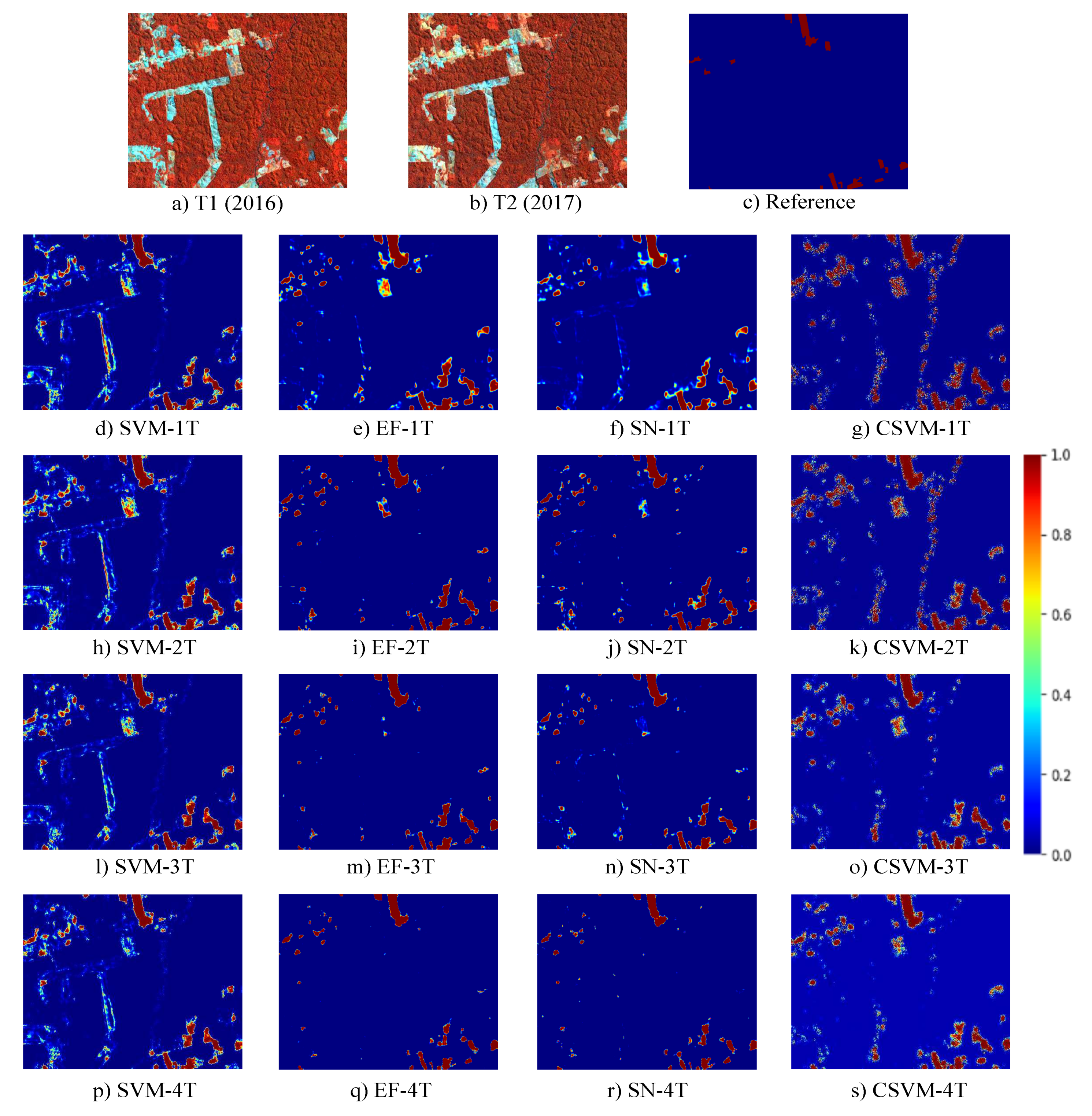
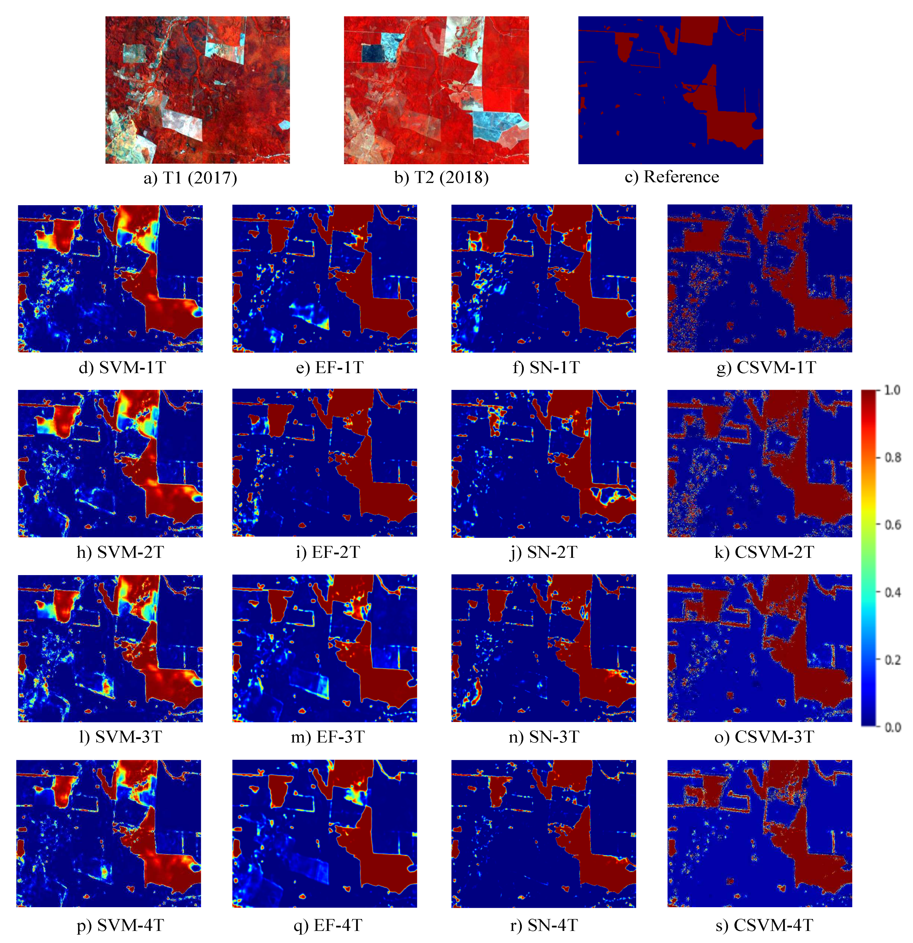
3. Results and Discussion
3.1. Amazon Biome
3.2. Alarm Area vs. Recall for Amazon Biome
3.3. Cerrado Biome
3.4. Alarm Area vs. Recall for Cerrado Biome
4. Conclusions
Author Contributions
Funding
Acknowledgments
Conflicts of Interest
References
- De Sy, V.; Herold, M.; Achard, F.; Beuchle, R.; Clevers, J.; Lindquist, E.; Verchot, L. Land use patterns and related carbon losses following deforestation in South America. Environ. Res. Lett. 2015, 10, 124004. [Google Scholar]
- MacDicken, K.; Jonsson, Ö.; Piña, L.; Maulo, S.; Contessa, V.; Adikari, Y.; Garzuglia, M.; Lindquist, E.; Reams, G.; D’Annunzio, R. Global Forest Resources Assessment 2015: How Are the World’s Forests Changing? Food and Agricultural Organization of the United Nations (FAO): Rome, Italy, 2015. [Google Scholar]
- Amin, A.; Choumert-Nkolo, J.; Combes, J.L.; Motel, P.C.; Kéré, E.N.; Ongono-Olinga, J.G.; Schwartz, S. Neighborhood effects in the Brazilian Amazônia: Protected areas and deforestation. J. Environ. Econ. Manag. 2019, 93, 272–288. [Google Scholar] [CrossRef]
- Aide, T.M.; Clark, M.L.; Grau, H.R.; López-Carr, D.; Levy, M.A.; Redo, D.; Bonilla-Moheno, M.; Riner, G.; Andrade-Núñez, M.J.; Muñiz, M. Deforestation and Reforestation of L atin A merica and the C aribbean (2001–2010). Biotropica 2013, 45, 262–271. [Google Scholar] [CrossRef]
- Brazilian Institute of Geography and Statistics (IBGE). Mapa de Biomas e de Vegetação. 2004. Available online: https://ww2.ibge.gov.br/home/presidencia/noticias/21052004biomashtml.shtm (accessed on 20 November 2019).
- Almeida, C.A.A.D.; Coutinho, A.C.; Esquerdo, J.A.C.A.D.M.; Adami, M.; Venturieri, A.; Diniz, C.G.; Dessay, N.; Durieux, L.; Gomes, A.R. High spatial resolution land use and land cover mapping of the Brazilian Legal Amazon in 2008 using Landsat-5/TM and MODIS data. Acta Amaz. 2016, 46, 291–302. [Google Scholar] [CrossRef]
- Sano, E.E.; Rosa, R.; Brito, J.L.A.s.S.; Ferreira, L.G.A. Mapeamento semidetalhado do uso da terra do Bioma Cerrado. Pesqui. Agropecuaria Bras. 2008, 43, 153–156. [Google Scholar] [CrossRef]
- Soterroni, A.C.; Ramos, F.M.; Mosnier, A.; Fargione, J.; Andrade, P.R.; Baumgarten, L.; Pirker, J.; Obersteiner, M.; Kraxner, F.; Câmara, G.; et al. Expanding the Soy Moratorium to Brazil’s Cerrado. Sci. Adv. 2019, 5. [Google Scholar] [CrossRef]
- Bueno, I.T.; Acerbi Júnior, F.W.; Silveira, E.M.; Mello, J.M.; Carvalho, L.M.; Gomide, L.R.; Withey, K.; Scolforo, J.R.S. Object-Based Change Detection in the Cerrado Biome Using Landsat Time Series. Remote Sens. 2019, 11, 570. [Google Scholar] [CrossRef]
- Goodman, R.; Aramburu, M.; Gopalakrishna, T.; Putz, F.; Gutiérrez, N.; Alvarez, J.; Aguilar-Amuchastegui, N.; Ellis, P. Carbon emissions and potential emissions reductions from low-intensity selective logging in southwestern Amazonia. For. Ecol. Manag. 2019, 439, 18–27. [Google Scholar] [CrossRef]
- Malingreau, J.; Eva, H.; De Miranda, E. Brazilian Amazon: a significant five year drop in deforestation rates but figures are on the rise again. Ambio 2012, 41, 309–314. [Google Scholar] [CrossRef]
- Barreto, P.; Souza, C., Jr.; Nogueron, R.; Anderson, A.; Salomão, R. Human Pressure on the Brazilian Amazon Forests; World Resources Institute: Washington, DC, USA, 2006. [Google Scholar]
- National Institute for Space Research (INPE). Monitoring of the Brazilian Amazonian Forest by Satellite. 1988. Available online: http://www.obt.inpe.br/OBT/assuntos/programas/amazonia/prodes (accessed on 5 November 2019).
- World Wildlife Fund (WWF). Amazon Deforestation. 1988. Available online: http://wwf.panda.org/our_work/forests/deforestation_fronts/deforestation_in_the_amazon/ (accessed on 7 December 2019).
- Ministry of the Environment (MMA); Brazilian Institute of Environment and Renewable Natural Resources (IBAMA). Monitoramento do desmatamento nos biomas brasileiros por satélite. 2011. Available online: http://www.mma.gov.br/estruturas/sbf_chm_rbbio/_arquivos/relatoriofinal_cerrado_2010_final_72_1.pdf (accessed on 15 November 2019).
- Assis, F.; Fernando, L.; Ferreira, K.R.; Vinhas, L.; Maurano, L.; Almeida, C.; Carvalho, A.; Rodrigues, J.; Maciel, A.; Camargo, C. TerraBrasilis: A Spatial Data Analytics Infrastructure for Large-Scale Thematic Mapping. ISPRS Int. J. -Geo-Inf. 2019, 8, 513. [Google Scholar] [CrossRef]
- Beuchle, R.; Grecchi, R.C.; Shimabukuro, Y.E.; Seliger, R.; Eva, H.D.; Sano, E.; Achard, F. Land cover changes in the Brazilian Cerrado and Caatinga biomes from 1990 to 2010 based on a systematic remote sensing sampling approach. Appl. Geogr. 2015, 58, 116–127. [Google Scholar] [CrossRef]
- Bonanomi, J.; Tortato, F.R.; Raphael de Souza, R.G.; Penha, J.M.; Bueno, A.S.; Peres, C.A. Protecting forests at the expense of native grasslands: Land-use policy encourages open-habitat loss in the Brazilian cerrado biome. Perspect. Ecol. Conserv. 2019, 17, 26–31. [Google Scholar] [CrossRef]
- Sathler, D.; Adamo, S.; Lima, E. Deforestation and local sustainable development in Brazilian Legal Amazonia: An exploratory analysis. Ecol. Soc. 2018, 23, 1–36. [Google Scholar] [CrossRef]
- National Institute for Space Research (INPE). Detecting Residential Land-Use Development at the Urban Fringe. 1982. Available online: https://www.asprs.org/wp-content/uploads/pers/1982journal/apr/1982_apr_629-643.pdf (accessed on 13 October 2019).
- Howarth, P.J.; Wickware, G.M. Procedures for change detection using Landsat digital data. Int. J. Remote Sens. 1981, 2, 277–291. [Google Scholar] [CrossRef]
- Ludeke, A.; Maggio, R.C.; Reid, L. An analysis of anthropogenic deforestation using logistic regression and GIS. J. Environ. Manag. 1990, 31, 247–259. [Google Scholar] [CrossRef]
- Nackaerts, K.; Vaesen, K.; Muys, B.; Coppin, P. Comparative performance of a modified change vector analysis in forest change detection. Int. J. Remote Sens. 2005, 26, 839–852. [Google Scholar] [CrossRef]
- Deng, J.S.; Wang, K.; Deng, Y.H.; Qi, G.J. PCA-based land-use change detection and analysis using multitemporal and multisensor satellite data. Int. J. Remote Sens. 2008, 29, 4823–4838. [Google Scholar] [CrossRef]
- Celik, T. Unsupervised change detection in satellite images using principal component analysis and k-means clustering. IEEE Geosci. Remote Sens. Lett. 2009, 6, 772–776. [Google Scholar] [CrossRef]
- Xiaolu, S.; Bo, C. Change detection using change vector analysis from Landsat TM images in Wuhan. Procedia Environ. Sci. 2011, 11, 238–244. [Google Scholar] [CrossRef]
- Zhan, Y.; Fu, K.; Yan, M.; Sun, X.; Wang, H.; Qiu, X. Change detection based on deep siamese convolutional network for optical aerial images. IEEE Geosci. Remote Sens. Lett. 2017, 14, 1845–1849. [Google Scholar] [CrossRef]
- Dhingra, S.; Kumar, D. A review of remotely sensed satellite image classification. Int. J. Electr. Comput. Eng. 2019, 9, 2088–8708. [Google Scholar] [CrossRef]
- Kranjčić, N.; Medak, D.; Župan, R.; Rezo, M. Support Vector Machine Accuracy Assessment for Extracting Green Urban Areas in Towns. Remote Sens. 2019, 11, 655. [Google Scholar] [CrossRef]
- Gunn, S.R. Support vector machines for classification and regression. ISIS Tech. Rep. 1998, 14, 5–16. [Google Scholar]
- Pal, M. Random forest classifier for remote sensing classification. Int. J. Remote Sens. 2005, 26, 217–222. [Google Scholar] [CrossRef]
- Maxwell, A.E.; Warner, T.A.; Fang, F. Implementation of machine-learning classification in remote sensing: An applied review. Int. J. Remote Sens. 2018, 39, 2784–2817. [Google Scholar] [CrossRef]
- Valeriano, D.M.; Mello, E.M.K.; Moreira, J.C.; Shimabukuro, Y.E.; Duarte, V.; Souza, I.M.; dos Santos, J.R.; Barbosa, C.C.F.; de Souza, R.C.M. Monitoring tropical forest from space: The PRODES digital project. Int. Arch. Photogramm. Remote Sens. Spat. Inf. Sci. 2004, 35, 272–274. [Google Scholar]
- National Institute for Space Research (INPE). Metodologia Utilizada nos Projetos Prodes e Deter. Available online: http://www.obt.inpe.br/OBT/assuntos/programas/amazonia/prodes/pdfs/Metodologia_Prodes_Deter_revisada.pdf (accessed on 15 October 2019).
- Kintisch, E. Improved monitoring of rainforests helps pierce haze of deforestation. Science 2007, 316, 536–537. [Google Scholar] [CrossRef]
- Shimabukuro, Y.; Duarte, V.; Anderson, L.; Valeriano, D.; Arai, E.; Freitas, R.; Rudorff, B.F.; Moreira, M. Near real time detection of deforestation in the Brazilian Amazon using MODIS imagery. Ambiente Agua Interdiscip. J. Appl. Sci. 2007, 1, 37–47. [Google Scholar] [CrossRef]
- Brito, A.; Valeriano, D.D.M.; Ferri, C.; Scolastrici, A.; Sestini, M. Metodologia da detecção do desmatamento no bioma Cerrado. In Mapeamento de Áreas Antropizadas Com Imagens de Média Resolução Espacial; Instituto Nacional de Pesquisas Espaciais: São José dos Campos, Brazil, 2018. [Google Scholar]
- Souza, C.; Azevedo, T. MapBiomas General Handbook; MapBiomas: São Paulo, Brazil, 2017; pp. 1–23. [Google Scholar]
- Machado, R.B.; Ramos Neto, M.B.; Pereira, P.G.P.; Caldas, E.F.; Gonçalves, D.A.; Santos, N.S.; Tabor, K.; Steininger, M. Estimativa de Perda da Área do Cerrado Brasileiro; Relatório Técnico Não Publicado; Conservação Internacional: Brasília, Brazil, 2004; pp. 1–25.
- Picoli, M.C.A.; Camara, G.; Sanches, I.; Simões, R.; Carvalho, A.; Maciel, A.; Coutinho, A.; Esquerdo, J.; Antunes, J.; Begotti, R.A.; et al. Big earth observation time series analysis for monitoring Brazilian agriculture. ISPRS J. Photogramm. Remote Sens. 2018, 145, 328–339. [Google Scholar] [CrossRef]
- Zagoruyko, S.; Komodakis, N. Learning to compare image patches via convolutional neural networks. In Proceedings of the IEEE Conference on Computer Vision and Pattern Recognition, Boston, MA, USA, 7–12 June 2015; pp. 4353–4361. [Google Scholar]
- Daudt, R.C.; Le Saux, B.; Boulch, A.; Gousseau, Y. Urban change detection for multispectral earth observation using convolutional neural networks. In Proceedings of the IGARSS 2018—2018 IEEE International Geoscience and Remote Sensing Symposium, Valencia, Spain, 22–27 July 2018; pp. 2115–2118. [Google Scholar]
- Zhang, Z.; Vosselman, G.; Gerke, M.; Tuia, D.; Yang, M.Y. Change detection between multimodal remote sensing data using siamese CNN. arXiv 2018, arXiv:1807.09562. [Google Scholar]
- Mou, L.; Bruzzone, L.; Zhu, X. Learning spectral-spatial-temporal features via a recurrent convolutional neural network for change detection in multispectral imagery. IEEE Trans. Geosci. Remote Sens. 2019, 57, 924–935. [Google Scholar] [CrossRef]
- Lovett, G.M.; Burns, D.A.; Driscoll, C.T.; Jenkins, J.C.; Mitchell, M.J.; Rustad, L.; Shanley, J.B.; Likens, G.E.; Haeuber, R. Who needs environmental monitoring? Front. Ecol. Environ. 2007, 5, 253–260. [Google Scholar] [CrossRef]
- Rahman, F.; Vasu, B.; Van Cor, J.; Kerekes, J.; Savakis, A. Siamese Network with Multi-Level Features for Patch-Based Change Detection in Satellite Imagery. In Proceedings of the 2018 IEEE Global Conference on Signal and Information Processing (GlobalSIP), Anaheim, CA, USA, 26–29 November 2018; pp. 958–962. [Google Scholar]
- Bazi, Y.; Melgani, F. Convolutional SVM networks for object detection in UAV imagery. IEEE Trans. Geosci. Remote Sens. 2018, 56, 3107–3118. [Google Scholar] [CrossRef]
- Casseb, A.d.R.; Chiang, J.O.; Martins, L.C.; Silva, S.P.d.; Henriques, D.F.; Casseb, L.M.N.; Vasconcelos, P.F.d.C. Alphavirus serosurvey in domestic herbivores in Pará State, Brazilian Amazon. Rev. Pan-Amazônica Saúde 2012, 3, 43–48. [Google Scholar] [CrossRef]
- Steinweg, T.; Gerard, R.; Thoumi, G. Cargill: Zero-Deforestation Approach Leaves Room for Land Clearing in Brazil’s Maranhão. In Chain Reaction Research. 2018, pp. 1–18. Available online: https://chainreactionresearch.com/wp-content/uploads/2018/04/Cargill-report-April-2018.pdf (accessed on 20 November 2019).
- Fan, R.E.; Chang, K.W.; Hsieh, C.J.; Wang, X.R.; Lin, C.J. LIBLINEAR: A library for large linear classification. J. Mach. Learn. Res. 2008, 9, 1871–1874. [Google Scholar]


| Set | Tiles | Available Def. Samples | Available No-def. Samples | Balanced Samples (per Class) | Total Samples |
|---|---|---|---|---|---|
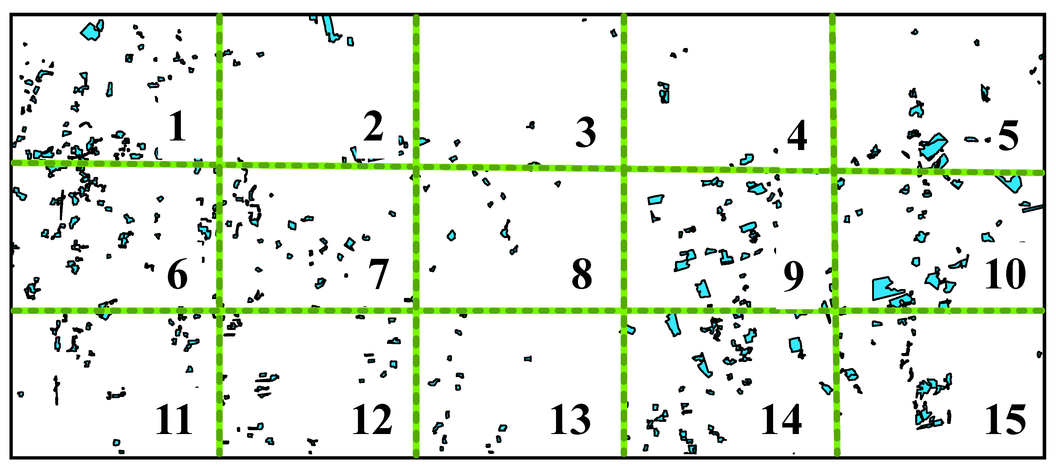
| Training | 1, 7, 9, 13 | 2706 | 78,431 | 8118 | 16,236 |
| Validation | 5, 12 | 963 | 39,697 | 2889 | 5778 |
| Test | 2, 3, 4, 6, 8, 10, 11, 14, 15 | 40,392 | 1,675,608 | - | 1,716,000 |
| Set | Tiles | Available Def. Samples | Available No-def. Samples | Balanced Samples (per Class) | Total Samples |
|---|---|---|---|---|---|
| Training | 1, 5, 12, 13 | 4182 | 65,717 | 12,546 | 25,092 |
| Validation | 6, 10 | 663 | 34,658 | 1989 | 3978 |
| Test | 2, 3, 4, 7, 8, 9, 11, 14, 15 | 68,983 | 1,416,278 | - | 1,485,261 |
| Layer | Filter Size | Output Size | Parameters |
|---|---|---|---|
| Input | - | 15 × 15 × 16 | - |
| Conv1 | 3 × 3 | 15 × 15 × 128 | 18,560 |
| MaxPool1 | 2 × 2 | 7 × 7 × 128 | - |
| Conv2 | 3 × 3 | 7 × 7 × 256 | 295,168 |
| MaxPool2 | 2 × 2 | 3 × 3 × 256 | - |
| Conv3 | 3 × 3 | 3 × 3 × 512 | 1,180,160 |
| FC1 | - | 1 × 4608 | - |
| Dropout | - | 1 × 4608 | - |
| FC2 | - | 1 × 2 | 9218 |
| Total params | - | - | 1,503,106 |
| Treinable params | - | - | 1,503,106 |
| Layer | Filter Size | Output Size | Parameters |
|---|---|---|---|
| Input | - | 15 × 15 × 8 | - |
| Conv1 | 3 × 3 | 15 × 15 × 128 | 9344 |
| MaxPool1 | 2 × 2 | 7 × 7 × 128 | - |
| Conv2 | 3 × 3 | 7 × 7 × 256 | 295,168 |
| MaxPool2 | 2 × 2 | 3 × 3 × 256 | - |
| Conv3 | 3 × 3 | 3 × 3 × 512 | 1,180,160 |
| FC1 | - | 1 × 4608 | - |
| Concatenation | - | 1 × 9216 | - |
| Dropout | - | 1 × 9216 | - |
| FC2 | - | 1 × 2 | 18,434 |
| Total params | - | - | 1,503,106 |
| Treinable params | - | - | 1,503,106 |
| Layer | Filter Size | Output Size | Parameters |
|---|---|---|---|
| Input | - | 15 × 15 × 16 | - |
| Conv1 | 3 × 3 | 13 × 13 × 12 | 1740 |
| MaxPool1 | 1 × 1 | 11 × 11 × 12 | - |
| Conv2 | 3 × 3 | 9 × 9 × 12 | 1308 |
| MaxPool2 | 1 × 1 | 7 × 7 × 12 | - |
| Conv3 | 3 × 3 | 5 × 5 × 12 | 1308 |
| MaxPool3 | 1 × 1 | 3 × 3 × 15 | - |
| Total params | - | - | 4356 |
| Treinable params | - | - | 4356 |
| Training Set | Tiles | Available Def. Samples | Available No-def. Samples | Balanced Samples (per Class) | Total Samples (tr + val) |
|---|---|---|---|---|---|
| 1 Tile | 13 | 239 | 20,306 | 717 | 1434 + 5778 |
| 2 Tiles | 1, 13 | 709 | 40,515 | 2127 | 4254 + 5778 |
| 3 Tiles | 1, 7, 13 | 1807 | 59,102 | 5421 | 10,842 + 5778 |
| 4 Tiles | 1, 7, 9, 13 | 2706 | 78,431 | 8118 | 16,236 + 5778 |
| Training Set | Tiles | Available Def. Samples | Available No-def. Samples | Balanced Samples (per Class) | Total Samples (tr + val) |
|---|---|---|---|---|---|
| 1 Tile | 5 | 671 | 17,370 | 2013 | 4026 + 3,978 |
| 2 Tiles | 5, 13 | 1240 | 33,760 | 3720 | 7440 + 3,978 |
| 3 Tiles | 1, 5, 13 | 2287 | 50,273 | 6861 | 13,722 + 3,978 |
| 4 Tiles | 1, 5, 12, 13 | 4182 | 65,717 | 12,546 | 25,092 + 3978 |
© 2020 by the authors. Licensee MDPI, Basel, Switzerland. This article is an open access article distributed under the terms and conditions of the Creative Commons Attribution (CC BY) license (http://creativecommons.org/licenses/by/4.0/).
Share and Cite
Ortega Adarme, M.; Queiroz Feitosa, R.; Nigri Happ, P.; Aparecido De Almeida, C.; Rodrigues Gomes, A. Evaluation of Deep Learning Techniques for Deforestation Detection in the Brazilian Amazon and Cerrado Biomes From Remote Sensing Imagery. Remote Sens. 2020, 12, 910. https://doi.org/10.3390/rs12060910
Ortega Adarme M, Queiroz Feitosa R, Nigri Happ P, Aparecido De Almeida C, Rodrigues Gomes A. Evaluation of Deep Learning Techniques for Deforestation Detection in the Brazilian Amazon and Cerrado Biomes From Remote Sensing Imagery. Remote Sensing. 2020; 12(6):910. https://doi.org/10.3390/rs12060910
Chicago/Turabian StyleOrtega Adarme, Mabel, Raul Queiroz Feitosa, Patrick Nigri Happ, Claudio Aparecido De Almeida, and Alessandra Rodrigues Gomes. 2020. "Evaluation of Deep Learning Techniques for Deforestation Detection in the Brazilian Amazon and Cerrado Biomes From Remote Sensing Imagery" Remote Sensing 12, no. 6: 910. https://doi.org/10.3390/rs12060910
APA StyleOrtega Adarme, M., Queiroz Feitosa, R., Nigri Happ, P., Aparecido De Almeida, C., & Rodrigues Gomes, A. (2020). Evaluation of Deep Learning Techniques for Deforestation Detection in the Brazilian Amazon and Cerrado Biomes From Remote Sensing Imagery. Remote Sensing, 12(6), 910. https://doi.org/10.3390/rs12060910