Abstract
Due to their motion, floating wind lidars overestimate turbulence intensity () compared to fixed lidars. We show how the motion of a floating continuous-wave velocity–azimuth display (VAD) scanning lidar in all six degrees of freedom influences the estimates, and present a method to compensate for it. The approach presented here uses line-of-sight measurements of the lidar and high-frequency motion data. The compensation algorithm takes into account the changing radial velocity, scanning geometry, and measurement height of the lidar beam as the lidar moves and rotates. It also incorporates a strategy to synchronize lidar and motion data. We test this method with measurement data from a ZX300 mounted on a Fugro SEAWATCH Wind LiDAR Buoy deployed offshore and compare its estimates with and without motion compensation to measurements taken by a fixed land-based reference wind lidar of the same type located nearby. Results show that the values of the floating lidar without motion compensation are around higher than the reference values. The motion compensation algorithm detects the amount of motion-induced and removes it from the measurement data successfully. Motion compensation leads to good agreement between the estimates of floating and fixed lidar under all investigated wind conditions and sea states.
1. Introduction
Wind velocity measurements are important for the wind energy industry to validate assumptions about wind conditions at a wind farm site. Lidar measurements that sense the wind remotely from the ground can be used instead of in-situ anemometry on meteorological masts. The installation of such masts offshore is even more expensive than onshore. As wind projects move further offshore into deeper water areas, masts are no longer a feasible alternative. Floating lidars are more cost-effective than masts [1] and potentially the only viable option. Validation campaigns testing floating lidar systems against data from meteorological masts have shown that estimations of the mean wind velocity by floating lidar are robust and reliable [2,3]. Even without any form of motion compensation, the errors in mean wind speed are small [4,5,6]. For estimates of the wind direction, a simple yaw compensation at the ten-minute level is sufficient [2].
By contrast, estimates of turbulence intensity () require advanced motion compensation because floating lidar systems show stronger wind velocity fluctuations than non-moving lidars [5]. The magnitude of this motion-induced error depends on the amplitude and period of the motion which result from the floating platform type used and the prevailing sea state [7]. Trusting in such erroneously high values could, for example, result in extra costs caused by choosing overdesigned wind turbines. Different methods have therefore been proposed to mitigate or remove the motion-induced error in estimates from floating lidar systems.
As suggested in Tiana-Alsina et al. [8], the lidar device could be mounted on a cardanic frame that compensates for most of the rotational motion. Such a hardware solution increases the costs for a floating lidar system and cannot compensate for errors that are caused by significant translational motion of the platform; for example, those due to heave caused by waves. Gutiérrez et al. [9] proposed simple window averaging of the time series of horizontal wind speed estimates, which acts as a low-pass filter. The basic idea is that the motion-induced turbulence has the same frequency as the buoy motion and can therefore be filtered out. The main drawback of this method is that the sampling frequency of the lidar-measured time series must be higher than the frequency of the motion of the platform. For many setups with currently available hardware, this is not the case. Gutiérrez-Antunano et al. [7] presented a simulation tool for more advanced motion compensation. Based on amplitude and period of the buoy rotation, and mean wind conditions, the simulator estimates the motion-induced error in the turbulence measurements. Corrected measurement data show overall better results compared to reference lidar measurements, but the success of the method varies depending on sea state. Yamaguchi and Ishihara [10] suggested a motion compensation algorithm based on numerical simulations that shows promising results. However, the method requires simultaneously measured line-of-sight velocities from different measurement heights, which are available only from pulsed wind lidars. Gottschall et al. [5] described a motion compensation algorithm to correct for the rotation of a floating pulsed wind lidar in roll, pitch, and yaw degrees of freedom and show promising results. In Gottschall et al. [11], they describe an algorithm that corrects the lidar derived line-of-sight velocities for the influence of motion in all six degrees of freedom but do not disclose any details of the algorithm and do not describe the motion-corrected results.
The aim of the work presented here was to develop and validate a method that corrects estimates from a floating continuous-wave wind lidar aboard a buoy being deployed offshore. For our approach, we measure the motion of the buoy in all six degrees of freedom and record the line-of-sight velocity spectra of the lidar. We then compensate for the motion of the lidar before we reconstruct the wind vectors under consideration of the rotation of the buoy. A method to synchronize the lidar and motion data is an integral feature of our approach. We applied this motion compensation algorithm to measurement data from a SEAWATCH Wind LiDAR Buoy by Fugro carrying a ZX300M by ZX Lidar (Ledbury, United Kingdom) and a MRU 6000 motion reference unit (MRU) by Norwegian Subsea (Oslo, Norway) and analyzed the results in comparison to data from a nearby land-based fixed reference lidar of the same type. The scope of this work is the question of whether a motion-compensated floating lidar system can measure as reliably as a fixed reference lidar of the same type. is the most widely-used parameter of turbulence. We will therefore limit our analysis to it after briefly presenting the horizontal mean wind speeds. This article does not discuss the effects that lead to deviations between lidar-derived turbulence estimates and in-situ anemometric values [12,13,14].
In Section 2, we describe the theory behind , the coordinate systems we use, and how the motion of a velocity–azimuth display (VAD) scanning wind lidar influences its measurements. Section 3 describes our method to compensate for the lidar motion. This includes an explanation of how to overcome the challenge of synchronizing the timing of lidar and motion data and how we emulated the internal data processing of the lidar, which is typically not accessible. We also describe the measurement setup and describe the wind and sea conditions during the experimental validation. The results of the measurements are shown and discussed in Section 4 and we conclude the findings of this study in Section 5. Readers who do not seek to understand how the motion compensation algorithm works but are interested in its validation can continue reading from Section 3.5.
2. Theory
2.1. Turbulence Intensity
Wind velocities at one point in space can be described by the vector
where is the longitudinal component of the horizontal wind velocity in mean wind direction clockwise from north , is the transversal component of the horizontal wind velocity, and is the vertical wind velocity component in a right-handed coordinate system. The mean wind conditions are determined by averaging the values of for a time interval. The ZX300 wind lidar stores the time series of reconstructed wind vectors in the form of, first, the horizontal wind speed ; second, the wind direction ; and third, the vertical wind speed . In our analysis we look at ten-minute intervals of wind data. The average wind speed is the arithmetic mean of all N estimates of within each interval according to
As a measure for the amount of variation of around , we introduce the standard deviation of the horizontal wind speed
which is an indicator of turbulence. Since turbulence is partly driven by frictional forces caused by the mean wind speed, we normalize the wind speed variations by the mean wind speed , which leads us to the definition of turbulence intensity:
increases with surface roughness and decreases with height above ground [15]. Thermal buoyancy forces are the second driver of turbulence. Their influence leads to high values at low wind speeds. Unstable atmospheric stratification is also associated with high values, while stable conditions decrease it.
2.2. Coordinate System and Vector Rotations
The SEAWATCH Wind LiDAR Buoy is depicted in Figure 1. The buoy is anchored to the seabed with a catenary mooring line and floats on the water’s surface. In its initial position without the influence of any wave, wind or current loads, its x, y, and z-axes are respectively pointing north, east, and vertically down. In the presence of external forces, the buoy can move in all six degrees of freedom. Translational motion in x, y, and z-directions is called surge, sway, and heave, respectively. The horizontal distances are limited by the mooring system, and the vertical heave position follows waves and the tide. Rotations around these three axes are called roll, pitch, and yaw, respectively. The rotation in roll and pitch can be combined and their Pythagorean sum is then called tilt. The motion in roll, pitch, and heave is mostly determined by the sea state, as the buoy follows the wave motion with its characteristic periodicity. Surge, sway, and yaw motions typically occur with much longer periods and are mostly caused by wind and current forces that balance out the restoring forces from the mooring.
Figure 1.
Visualization of the SEAWATCH Wind LiDAR Buoy in pitched orientation. Shown are the global right-handed North-West-Up (NWU) coordinate system and the north-east-down (NED) reference frame of the motion reference unit (MRU) (gray); unit vectors , , and along the rotated body coordinate axes of the (MRU) (blue); unit vectors , , and defining the lidar frame of reference (red); the line-of-sight (LOS) unit vector for the azimuth offset angle (green); and the LOS unit vector for an arbitrary (yellow). Additionally, the separation vector between the MRU and lidar prism is shown, as are the nominal and real azimuth ( and ) and zenith angles ( and ). (Sketch not to scale).
For our computations, we use a global right-handed Cartesian north-west-up (NWU) coordinate system. The MRU we use in this study is set up to calculate and record translational and rotational position and velocity data in all six degrees of freedom; namely, translations in surge, sway, and heave, and the Tait–Bryan angles roll, pitch, and yaw. The motion data is based on a right-handed north-east-down coordinate system. The MRU is located approximately below the rotating prism of the lidar. The lidar is positioned parallel to the x–y plane of the MRU but its heading is rotated around the z-axis by from the x-direction towards the y-direction. Information about the direction of each line-of-sight measurement relative to the lidar frame of reference is given in the form of the fixed zenith angle and the azimuth angle relative to the heading of the lidar. A series of vector rotations is required to transform this information and the orientation data, i.e., roll, pitch, and yaw angles, R, P, and Y, measured by the MRU, into information about the real zenith angle and real azimuth angle of the lidar beam in the global coordinate system. The unit vector in the x-direction of the MRU in global NWU coordinates after rotation is in accordance with C.3.8 in Grewal et al. [16] given by
The unit vector in the y-direction of the MRU in NWU coordinates after rotation is given by
The unit vector in the z-direction of the MRU in NWU coordinates after rotation is given by
points downwards. We change its sign to create a unit vector that points upwards into the direction of the laser beam before it is deflected by the lidar prism.
, the unit vector in the direction of the lidar heading is determined by rotating by the yaw-offset angle around . This can be done by multiplying by the rotation matrix
where is the axis of rotation and the angle of rotation. A derivation of Equation (9) can be found in Section 9.2 of Cole [17]. In order find the unit vector we simply use
, the unit vector that points into the line-of-sight direction for is defined by rotating by the half cone opening angle around . The unit vector for a line-of-sight measurement at a particular azimuth angle is found by rotating by the negative azimuth angle around .
The real zenith angle is the angle between the vertical up direction and the line-of-sight measurement direction. It can deviate from when the buoy is rotated and can be determined by
where is the unit vector in the upwards direction. The real azimuth angle is the angle between the horizontal north direction and the projection of the line-of-sight measurement direction onto the horizontal plane. It can be determined by
where is the unit vector in the north direction. The sign of must be switched for .
The next task is to determine the influence of the buoy motion on the line-of-sight velocities. We first calculate the velocity vector of the lidar at the position of its prism and define the distance vector
that separates the location of motion measurement from the location of the lidar prism. The velocity at the lidar prism is the sum of the translational velocities measured at the location of the MRU and the rigid body motion caused by the angular velocity measured at the MRU location according to
The selection of the unit vectors , , and where the subscript stands for “down” corresponds to the orientation of the velocity data , , and , as defined in the setup of the MRU. The terms for the influence of roll and pitch angular velocity and on the translational velocity are sufficient when the distance vector is oriented along the z-axis of the MRU. If contains non-zero elements for the first or second coordinate, a third term for azimuthal rotation is required.
As a last step, the velocity vector must be projected onto the line-of-sight unit vector so that
is the projection of the translational velocity onto the line-of-sight unit vector. is the motion-induced error in the line-of-sight velocity caused by motion.
2.3. The Motion-Induced Error in TI Measurements
Reconstructed wind vectors from a moving and a fixed lidar system differ. In the following subsection, we categorize the measurement errors caused by lidar motion into three different effects.
2.3.1. Error in Radial Velocities due to Translational Motion
Translational motion of the lidar window in surge, sway, and heave according to Equation (14) changes the relative velocity between the emitted laser light and the scatterers. Thus, it shifts the detected Doppler frequency, which is proportional to the measured line-of-sight velocity. Stationary motion in the three translational degrees of freedom leads to a one-to-one change in measured wind velocity; e.g., a lidar being transported on a ship with velocity along the ocean’s surface would measure a wind velocity error of the same magnitude . With the exception of a lidar being mounted on a ship [18,19], all three velocity components of a floating lidar typically average zero during a ten-minute interval, so that . This leads to zero error in mean wind speed , but the measurements of the instantaneous wind speed and the derived turbulence parameters like are affected. The effect of translational motion on the instantaneous wind measurement is frequency dependent.
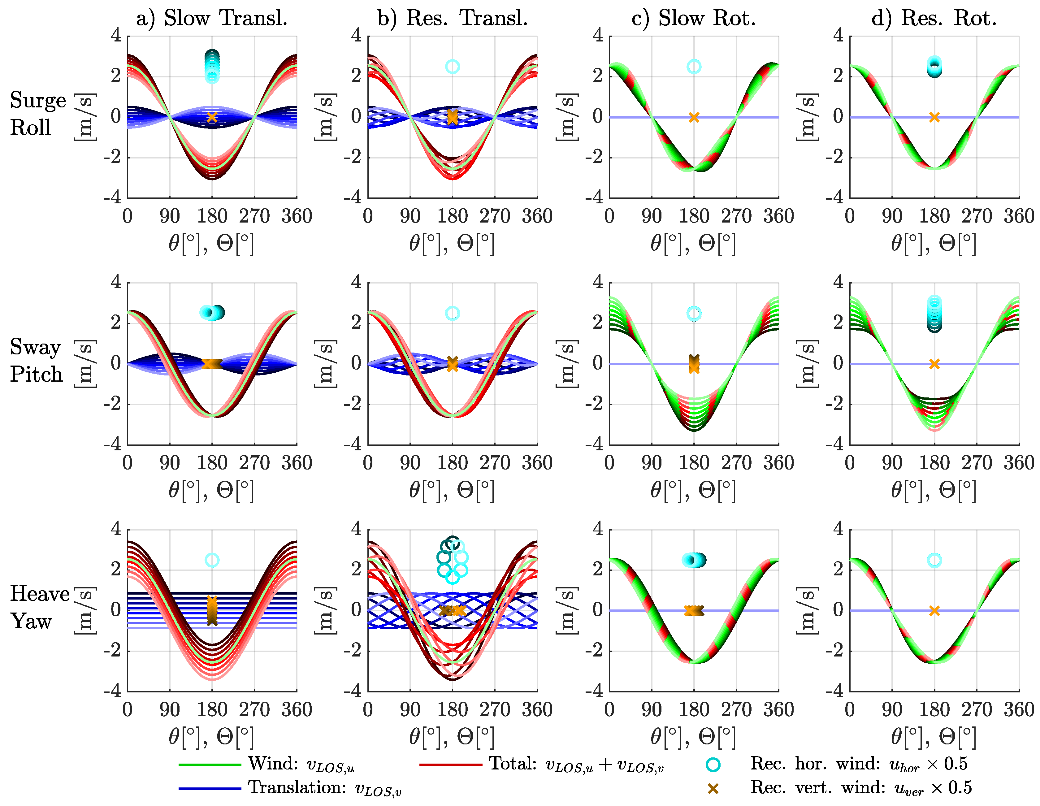
Oscillatory motion with a low frequency affects the wind component of the same orientation; i.e., the surge and sway components of motion and influence the horizontal wind speed components and ; heave velocity influences the vertical wind speed . Figure 2a shows this effect of translational motion. The figure shows line-of-sight velocities of a VAD scanning lidar on the y-axis plotted against the azimuth angle of the lidar beam on the x-axis. In all plots, the wind direction is assumed to be aligned with the heading of the lidar so that . The wind velocity is . We also define that surge motion occurs with an arbitrary amplitude of along the wind direction. Sway and heave have the same amplitude and are directed perpendicularly to the wind direction. The figure visualizes the lidar-measured LOS velocities in three ways: contribution of the wind, the lidar’s motion, and combined. The green lines represent the contribution of the wind to the line-of-sight measurement as if it were to be measured by a lidar without any translational motion. It has a cosine shape with peaks in the upward and downwind directions. The contribution of the translational motion on the line-of-sight velocities is visualized by the blue lines of varying darkness. The red lines show the sum of both contributions. We ignore that the lidar used in this study cannot detect the sign of the radial velocities. We therefore show the results of the wind vector reconstruction based on the absolute line-of-sight velocities according to Equations (20) and (21) as markers: cyan colored circle markers show the reconstructed horizontal wind speeds and brown cross markers show the reconstructed vertical wind speeds. Their location on the x-axis represents the reconstructed wind direction. It can be seen in Figure 2a that e.g., a slow back and forth motion in the wind direction (first row: surge) is detected in the same way as horizontal wind fluctuations; sideways motion (second row: sway) is perceived as transversal wind; and up and down motion (third row: heave) leads to a change of radial velocities in all line-of-sight directions. We see as expected that surge motion influences the horizontal wind speed ; sway motion influences the wind direction ; and heave motion leads exclusively to variation of the vertical wind speed component .
Figure 2.
Overview of the influence of motion on line-of-sight estimates and reconstructed wind vectors of a velocity–azimuth display (VAD) scanning floating lidar system. Shown are examples of translational motion with amplitude oscillating with frequency (a) and (b) , and the rotational motion of peak angle oscillating with (c) and (d) , where is the rotation frequency of the lidar prism. Green lines (dashed in c,d) are the radial velocity components of constant horizontal wind blowing in direction with a magnitude of as a function of the lidar azimuth angle . Blue lines are the influence of translational motion. Red lines are the total line-of-sight velocities. Color shades represent different phases of the oscillatory motion. Circle and cross markers represent the reconstructed wind vectors after conventional VAD processing, where the position on the y-axis is the magnitude and the position on the x-axis is the wind direction . More information in Section 2.3.1.
But these behaviors are valid only for translational motion that fluctuates very slowly; i.e., with a frequency much lower than one Hz, , which is the frequency of the rotating prism in the lidar corresponding to the time it takes to measure one full rotation of . Cross-contamination occurs for fluctuations that occur with a frequency close to this value. Cross-contamination in this context means that horizontal motion is interpreted as vertical wind speed fluctuations, and vertical buoy motion is interpreted as horizontal wind speed fluctuations. In other words, surge and sway motion of the buoy contribute to the estimates of vertical wind fluctuations, and heave motion is attributed to the fluctuations of horizontal wind; i.e., . We can see this in Figure 2 column b. The plots show what happens when translation occurs with a frequency of . We call this the “resonance case” because the azimuth angle and the magnitude of the surge/sway/heave velocity oscillate with the same frequency. While the azimuth angle of the laser beam rotates by , the sign of the motion velocity also changes. That means, the influence of motion on the line-of-sight velocities visualized in blue reaches its peak in this situation not after one full prism rotation as in the case of very slow fluctuations (see column a), but after every half rotation. As a consequence, the influence of motion is attributed to the wind velocity in a different orientation. Horizontal surge and sway motion in resonance leads to variations in vertical wind speed, and heave motion in resonance leads to variations in horizontal wind speed and wind direction. A lidar device with a half cone opening angle , like the one used in this study, is more sensitive to vertical heave motion than to horizontal motion in surge and sway. Heave in resonance therefore has a stronger influence on the horizontal wind speed than surge and sway have on the vertical wind speed.
From this analysis, we learn that heave motion in the resonance case and low-frequency fluctuations in surge and sway influence the estimates of a floating lidar. Heave motion must not be ignored because the period of waves is close enough to to create cross-contamination. Motion of the lidar in the surge and sway directions is not only created directly by translation of the buoy but also by tilting it when the center of rotation is not at the position of the lidar prism. Successful motion compensation therefore requires consideration of all degrees of freedom of motion.
2.3.2. Change in Scanning Geometry due to Rotational Motion
A second effect of motion-induced measurement errors on a floating lidar is caused by tilting of the platform. Rotations in pitch and roll directions change the real zenith angle of the lidar beam. For example, a beam with an increased real zenith angle has a higher sensitivity for the horizontal wind components than what is assumed in the internal wind vector reconstruction process using the constant half cone opening angle . Low-frequency tilting of the platform () can be imagined as tilting the complete measurement cone with its original half cone opening angle . The cone then has an increased real zenith angle on one side and a decreased real zenith angle on the other side. In such a situation, horizontal inflow causes the unsigned line-of-sight velocities to differ between the two sides of the cone. With the conventional VAD processing, horizontal wind is then misinterpreted as vertical wind. The third column c in Figure 2 visualizes this situation. Translational motion is no longer involved in these examples. Instead, we see that the steady inflow of horizontal wind leads to varying wind-induced line-of-sight velocities marked as dashed green lines due to the changing zenith angles . The magnitudes and shapes of these variations depend on the amplitude and orientation of the low-frequency tilt motion. Pitch motion (second row) leads to increased magnitude of the perceived wind velocity on one side of the measurement cone and a decreased value on the opposite side. Because no translational motion is involved, the total line-of-sight velocity marked in red is equal to the wind-induced line-of-sight velocity. The VAD processing leads to wind data that show nearly exclusively vertical turbulence. Roll rotation (first row) leads to a deviation from the sine shape of line-of-sight velocities but no systematic amplification on either side of the cone. The deviations result in an increased residual in the best-fit of the wind data reconstruction but do not lead to additional turbulence. Slow changes in the yaw angle (third row) lead to a phase shift in the line-of-sight velocities, and as a result, to varying wind directions but do not cause any error in because the estimates of stay the same. In summary, static misalignment and slow changes in the orientation do not have any influence on the estimates of .
However, when tilting occurs with a higher frequency close to , the measurement cone appears to become wider or narrower because the tilt angle of motion changes its sign as quickly as the lidar azimuth angle moves by to its opposite side. We can better understand this effect with the help of the plots in the last column d of Figure 2. Pitch motion in resonance with the lidar prism frequency (second row) can be understood as a stretched measurement cone with its maximum deviation from the original shape at the two ends that point into and against the mean wind direction. This geometry leads to either higher or lower sensitivity for the mean wind velocity on both sides of the cone at the same time. The result is increased horizontal turbulence in the reconstructed wind data. Rotations with resonance frequency in roll orientation (first row) also lead to increased turbulence in the wind data but to a lower extent than pitch rotations. The reason is that the apparently widened/narrowed cone has its maximum/minimum zenith angle at and where the beams point perpendicular to the wind inflow angle. Yawing with resonance frequency (third row) hardly occurs in reality, but it would have no effect on turbulence estimates. Instead, the cone averaging would swallow the resulting asymmetry in the line-of-sight velocities.
Static tilt leads to a decrease in mean wind speed, and dynamic tilting also has a small effect on mean wind speed that shall not be discussed here. We refer to Tiana-Alsina et al. [4] for more information. We have learned that dynamic tilting of the floating lidar that occurs with a frequency close to the lidar’s prism rotation frequency causes an increase in . The extent of this increase depends on the mean wind speed and the angle between wind direction and tilt orientation. By contrast, static and very low-frequency tilt motion, and yaw rotations, have no significant influence on the estimates.
2.3.3. Changing Measurement Elevation due to Rotation under the Influence of Wind Shear and Veer
Tilting the lidar not only leads to a changed scanning geometry, as described before in Section 2.3.2, but also leads to changing measurement elevations. If the horizontal mean wind speed and its direction were to be identical at all heights above the ground, this would not have any consequences for the turbulence measurements. But the presence of wind shear and veer, i.e., usually higher wind velocities at higher elevations and changing wind directions with height, respectively, leads to a third effect that is not captured in our above explanations. First, we look at the influence of wind shear. We ignore the elevation variations caused by heave motion because they are small and assume that the change in measurement elevation is exclusively created by tilting the lidar. When a lidar beam tilts towards the horizon, so that its zenith angle is increased, its sensitivity for the horizontal mean wind speed is also increased. Yet it measures the wind at a lower elevation, where the wind typically has lower horizontal mean speed. Conversely, a beam rotated towards the zenith measures a lower fraction of the horizontal mean wind speed, which is typically increased at the higher measurement elevation. That means, the effect of wind shear is always directed against the effect of changed scanning geometry. We can determine the relative magnitude between the two effects.
is the change in line-of-sight velocity of a beam pointing into the direction of the mean wind U with a half cone opening angle of that is tilted by tilt angle towards the horizon. This equation does not consider wind shear and represents only the changed scanning geometry, and therefore, the subscript that refers to the second effect described in this section. With z being the initial measurement elevation, we can calculate the change in elevation according to
The change in line-of-sight velocity that considers not only the changed geometry as in Equation (16) but also the wind shear is
With these equations, we can define a wind shear reduction factor
where the numerator is the change in line-of-sight velocity for a rotation from to when wind shear is considered. The denominator describes the same but without considering wind shear. As a result, k is the factor by which the effect of changed scanning geometry is reduced by the effect of wind shear. Measured mean wind velocities can be used to create wind profiles by linear inter and extrapolation. The resulting wind shear reduction factor is usually low. We found out that the dependency of k on the tilt angle is low, and it varies more with the measurement height z. Based on the measurement data used for this study, we calculated the average values for all height levels z and tilt angles to be %. We therefore assume that the effect of wind shear compensates for this amount of the effect of changed scanning geometry. The effect of wind veer might increase the measured turbulence again to some unknown extent. The effect is difficult to quantify, because wind veer involves dynamic changes in the wind direction which lead to significant deviations from the figures-of-eight, as explained in Section 2.3.2. However, we consider wind veer in the motion compensation algorithm that we present in Section 3.2.
All three effects described in this section are fully independent of the line-of-sight averaging. That means motion-compensated wind statistics will miss the same amount of turbulence due to averaging along the lines-of-sight as their uncompensated counterparts. The time of approximately —during which the backscatter is accumulated for each line-of-sight Doppler spectrum—is so short that we assume the motion as static during this time.
Wolken-Möhlmann et al. [20] reported that the influence of rotation on the total error is stronger than the influence of translational motion, and our study supports this finding. Our computations also show that the error of shear and veer in turbulent fluctuations is nearly negligible, but its influence on the mean wind speed might be significant.
3. Method
3.1. Emulation of Conventional VAD Processing
The method we use in this study aims at eliminating the three previously described errors: firstly, by correcting the radial velocity measurements for the influence of the lidar translation; secondly, by employing a set of linear equations in the wind vector reconstruction process that consider the real azimuth and zenith angles; and lastly, by interpolating the mean wind speed and direction onto the actual measurement elevation. The method requires access to the radial velocity measurements for each line-of-sight. The ZX300M used for this study stores wind data on its internal hard drive by default for each reconstructed wind vector (“Wind_xxx@Y20yy_Mmm_Ddd.ZPH,” 1 files) and their average over a period of ten minutes (“Wind10_xxx@Y20yy_Mmm_Ddd.ZPH,” 10-min files). None of these standard output file types contains the required information about the line-of-sight wind velocities. We therefore used the software “Waltz™” to stream the Doppler spectra of all line-of-sight measurements to the hard drive of a connected computer. Files saved in this way have user-defined filenames with the ending .RAW.ZPH and can be extracted to readable comma separated files via Waltz. These files do not contain the radial velocities as such, but they contain the Doppler spectra for each line-of-sight measurement. In order to estimate the radial velocities from the spectra, we first calculated the mean and the standard deviation of the twenty bins of highest Doppler frequency (“FFTBin236” to “FFTBin255”) for each line-of-sight measurement. We assume that these high speed bins are not influenced by the wind under normal conditions but contain only noise. We then removed this noise floor from all bins by setting all spectral values to zero that are smaller than six of the standard deviations after subtracting the mean values from all bins. Of the resulting spectra we calculated the centroid bin and multiplied it by to get the radial velocities of each line-of-sight measurement [21,22]. We know from Pitter et al. [23] that the internal data processing algorithms are more advanced than what we describe here. It likely incorporates cloud detection and fog filters. Parameters for both are not known to us and can therefore not be imitated. Instead we use the unfiltered line-of-sight velocities.
Forty-nine line-of-sight measurements which were consecutively taken at one height level are the data basis for the reconstruction of each wind vector. From the radial velocities and associated azimuth angles , the three-dimensional wind data can be calculated by applying a least-squares fit to
where A, B, and C are parameters that contain the wind data according to
The sign ambiguity of the wind direction results from the use of unsigned line-of-sight velocities. It is resolved with the help of wind direction measurements of a local weather station, though flipping the sign of the wind vector neither influences the mean wind speed nor the turbulence intensity. As a next step, we compare the time series of wind data with the results of the internal data processing (i.e., the “Wind_xxx@Y20yy_Mmm_Ddd.ZPH” files) and filter out all values that are marked with a “9998” or “9999” flag by the ZX300. Wind data processed in this way were intended to be identical to the internally processed wind data. But a comparison shows deviations that are stronger and more frequent at higher elevation levels.
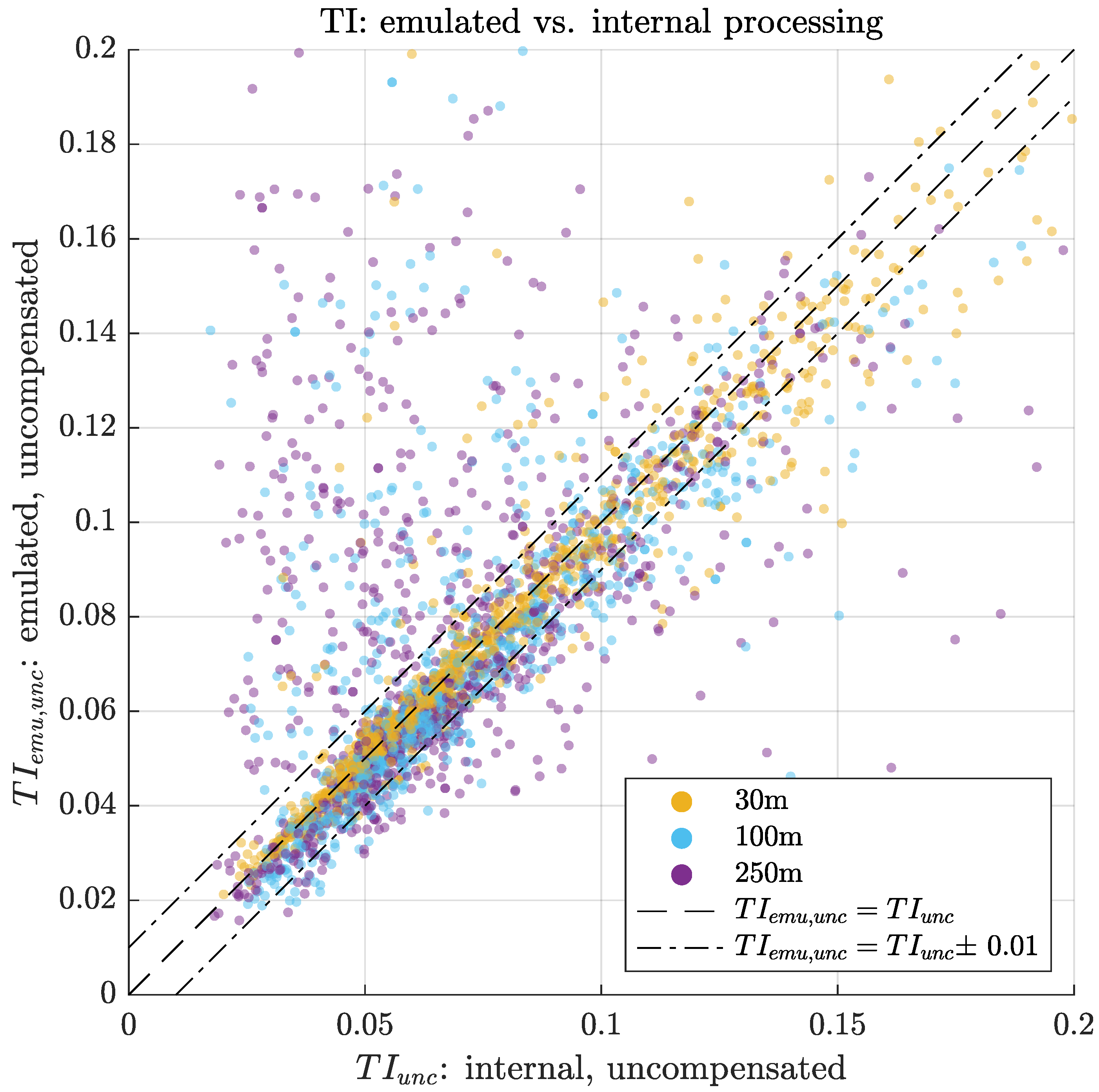
Figure 3 shows a scatter plot of values estimated from the time series of wind data of the floating lidar system. The values on the x-axis are based on horizontal wind velocities reconstructed by the internal data processing while the values on the y-axis are based on our own processing of the raw data, which emulates the internal processing. The figure shows an interval of around the 1:1 line. , , and of all values measured at , , and elevations respectively lie outside of this interval. This indicates that the simple centroid method we use for finding radial velocities deviates from the unknown method ZX lidar uses. An analysis of Doppler spectra which underlie the wind vectors showing the strongest deviations shows often double peaks that might indicate the presence of clouds. Therefore, we assume that the differences are mostly caused by filtering and cloud detection on a line-of-sight level and describe how we circumvent this problem in Section 3.4.
Figure 3.
Comparison of turbulence intensity () estimates based on wind data time series from internal data processing vs. emulated data processing. Only three height levels shown for clarity. The dashed-dotted lines limit a interval parallel to the dashed line.
3.2. The Motion Compensation Algorithm
The first challenge that must be addressed for applying motion compensation on a line-of-sight level involves the signs of the radial velocities. Radial wind velocity estimates from the ZX300 are unsigned. That means that air moving along a single laser beam away from the lidar cannot be differentiated from air moving towards the lidar, and the radial velocity is positive in both cases. In order to still be able to subtract the motion-induced velocity component, we must assign a sign to each line-of-sight velocity. We do this by reading the wind direction of each reconstructed wind vector and assigning a negative sign to the half of the line-of-sight measurements that point into the wind direction . This method requires that the mean wind determines the sign of the individual line-of-sight measurements and not turbulent fluctuations . This is an assumption which might be violated at azimuth angles that are close to orthogonal to the wind direction . These sideways beams hardly detect the mean wind but mostly the turbulence of the transversal and vertical wind velocity components. Mann et al. [24] and Dellwik et al. [25] report that radial velocity estimates from these directions are biased away from zero, and thus erroneous in any case. Additionally, in periods with very low mean wind speed, the assumption that the sign of radial velocities is determined by the wind direction could be violated. Here it should be noted that measurements of very low wind speeds are often of minor interest due to low power production and low structural loads associated with low wind speeds. Additionally, under unstable atmospheric conditions with high variance of the vertical wind speed component, sign errors are more likely because the sensitivity for vertical fluctuations is larger than the sensitivity for horizontal fluctuations because of the half-cone opening angle . The signed line-of-sight velocities can then be corrected for the influence of the buoy’s motion. First, the motion measured by the MRU in all six degrees of freedom must be projected onto unit vectors that point into the lidar beam direction according to Section 2.2. The magnitude of this projection is equal to the contribution of the motion to the radial velocity measurement, which we therefore subtract from the line-of-sight estimate.
In order to compensate for the effect of the lidar being rotated around its default orientation in roll, pitch, and yaw directions, the velocity–azimuth display wind vector reconstruction function (Equation (20)) is replaced by solving the following linear system
for u, v, and w where N is the number of line-of-sight measurements contributing to one measurement circle. Because in most cases, the linear system is overdetermined and must be solved using least squares. u and v are the two horizontal wind speed components oriented towards and respectively. Their Pythagorean sum is equal to and the angle they create is . w is equal to .
In order to compensate for the effect of wind shear and veer on the measurements, we determine the change in elevation due to rotation according to
for each line-of-sight. We must then interpolate the measured mean wind vectors at all measurement heights h to get a velocity profile that can be used to determine the resulting mean wind difference vector
which we multiply by the line-of-sight unit vector to get the value we eventually subtract from the measured line-of-sight velocity.
3.3. Time Synchronization
In order to correct the radial velocities for the influence of the motion, we must assign a timestamp to each line-of-sight measurement. This timestamp must, first, be related to the timestamp of the MRU, and second, be fine enough to resolve each line-of-sight measurement. In the default setup, two different types of temporal information are contained in the lidar raw data output: “timestamps” and “uptimems.” “Timestamps” contain information about date and time of each measurement, but they are updated only once per second, which is too coarse in the context of wave motion. “Uptimems” values, by contrast, assign a timestamp in milliseconds to each line-of-sight measurement, but these values use a different clock independent of the clock used for “timestamps.” “Uptimems” values are reset once the unit is switched off, and can therefore not be translated into date and time information directly. We decided to combine the information of both variables as follows. First, we select the first line-of-sight measurement of each day which has an updated “timestamps” but the same “reference” value as the one immediately preceding. All line-of-sight velocities that are used for one wind vector reconstruction have the same “reference” value. By using the same “reference” we avoid picking a line-of-sight measurement that is the first after the lidar refocuses to a new measurement height, which takes some unknown time. By doing so, we pick a line-of-sight measurement that was taken less than approximately after a new second of “timestamps” started. We then subtract the “uptimems” value of this measurement from all “uptimems” values of the whole day. To create new timestamps in milliseconds, we simply add the “timestamps” value of the selected measurement and these new “uptimems” values. When we compare the “uptimems” data with the original “timestamps” data over a longer period, we find that while 24 hours of “timestamps” time passes, on average less than 24 hours of “uptimems” time passes. That means that the newly created timestamps are finely resolved but contain the same drift per day relative to the lidar’s system time. We will solve this issue along with the synchronization of the MRU motion data and the lidar line-of-sight data.
Synchronization is crucial for successful motion compensation. The Doppler spectra of the lidar are streamed to an embedded PC, and the motion data is saved by means of a data acquisition system with a sample rate of . Both units are independently synchronized with a common GPS time server, but they are not synchronized with each other. Therefore, we expect an offset between the timestamps of the MRU and the lidar. To tackle this issue, we implement a method to synchronize the two measurement devices. Its underlying basic assumption is that the motion of the buoy caused by waves, current, and local wind is independent of the simultaneous wind vectors at measurement height. From this assumption it follows that the motion-induced error described in Section 2.3 and the current wind velocity are also independent variables. The turbulence measured by a floating lidar in motion must therefore be larger than measurements with a fixed lidar of the same type. The ideal motion compensation algorithm can reduce the measured turbulence down to exactly the level of a fixed lidar if the timing between motion and lidar data is correct. A timing error must lead to worse functionality; i.e., less compensation and consequently higher remaining turbulence. Due to the periodicity of ocean waves, the compensation can even become negative if the timing offset equals half the period length of the waves. In such a situation the algorithm would assume that the buoy is for example moving upwards although the real motion is directed downwards. The motion compensation would in that situation add turbulence instead of subtracting it. With these thoughts in mind, it is now simple to find the correct timing between MRU and lidar data. We need to calculate the motion compensation for different time lag values between MRU and lidar and determine the offset at which the motion-compensated turbulence reaches its minimum.
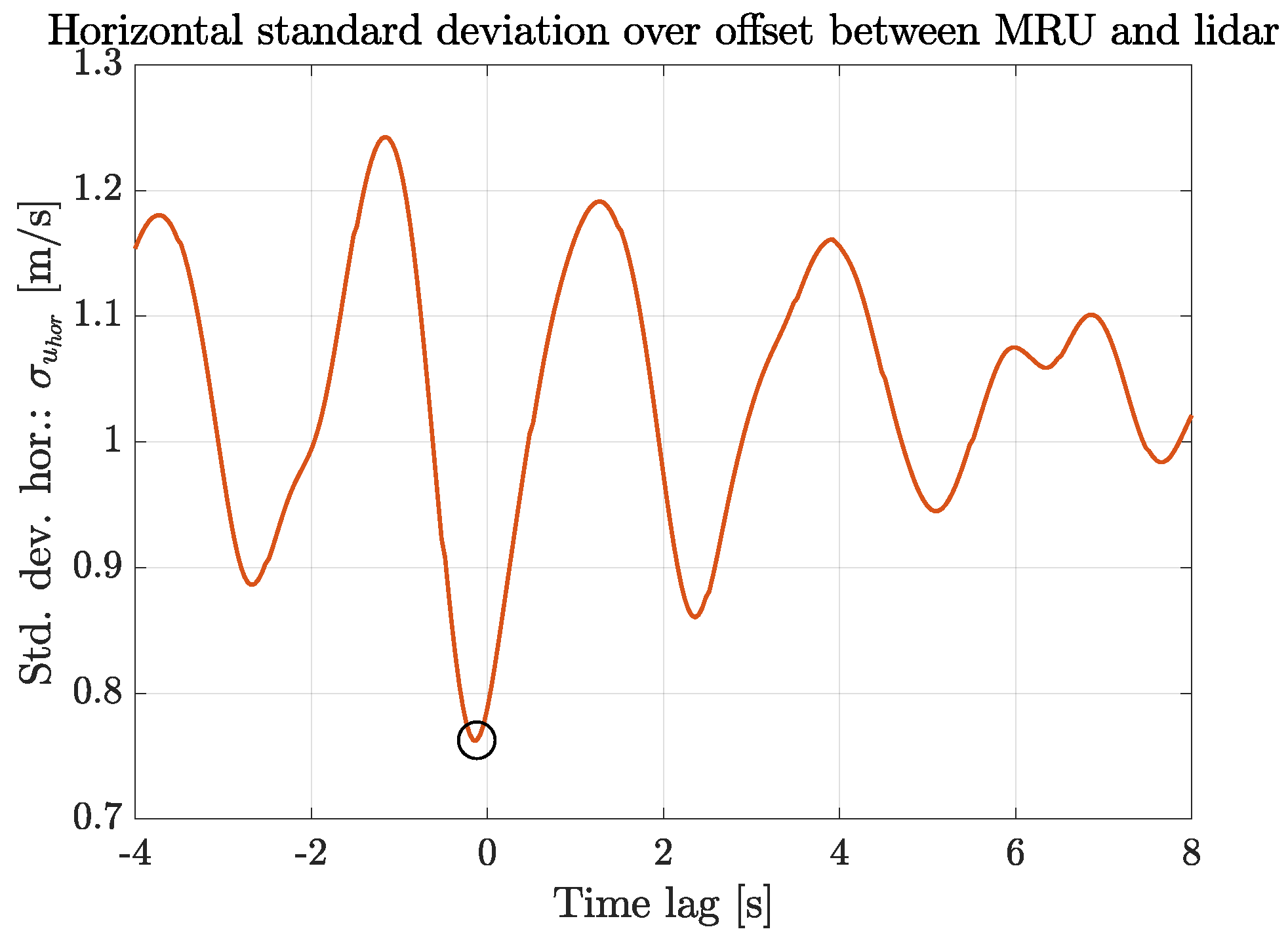
Figure 4 shows the result of this procedure for an arbitrary ten-minute interval. The y-axis shows motion-corrected standard deviation values of the horizontal wind speed averaged over all measurement heights. The corresponding time lag between lidar and MRU timestamp is shown on the x-axis. The absolute minimum is found at . This is the average offset between lidar and MRU data for this ten-minute interval. The periodicity of the waves is visible, and leads to local minima each separated by approximately . These local minima must not be confused with the absolute minimum, which is the sweet spot we aim for.
Figure 4.
Standard deviation of the motion compensated horizontal wind speed as a function of timing offset between MRU and lidar data. is the mean of all height levels for one arbitrary ten-minute interval. The absolute minimum at indicates the sweet spot that corresponds to the real offset between the two datasets.
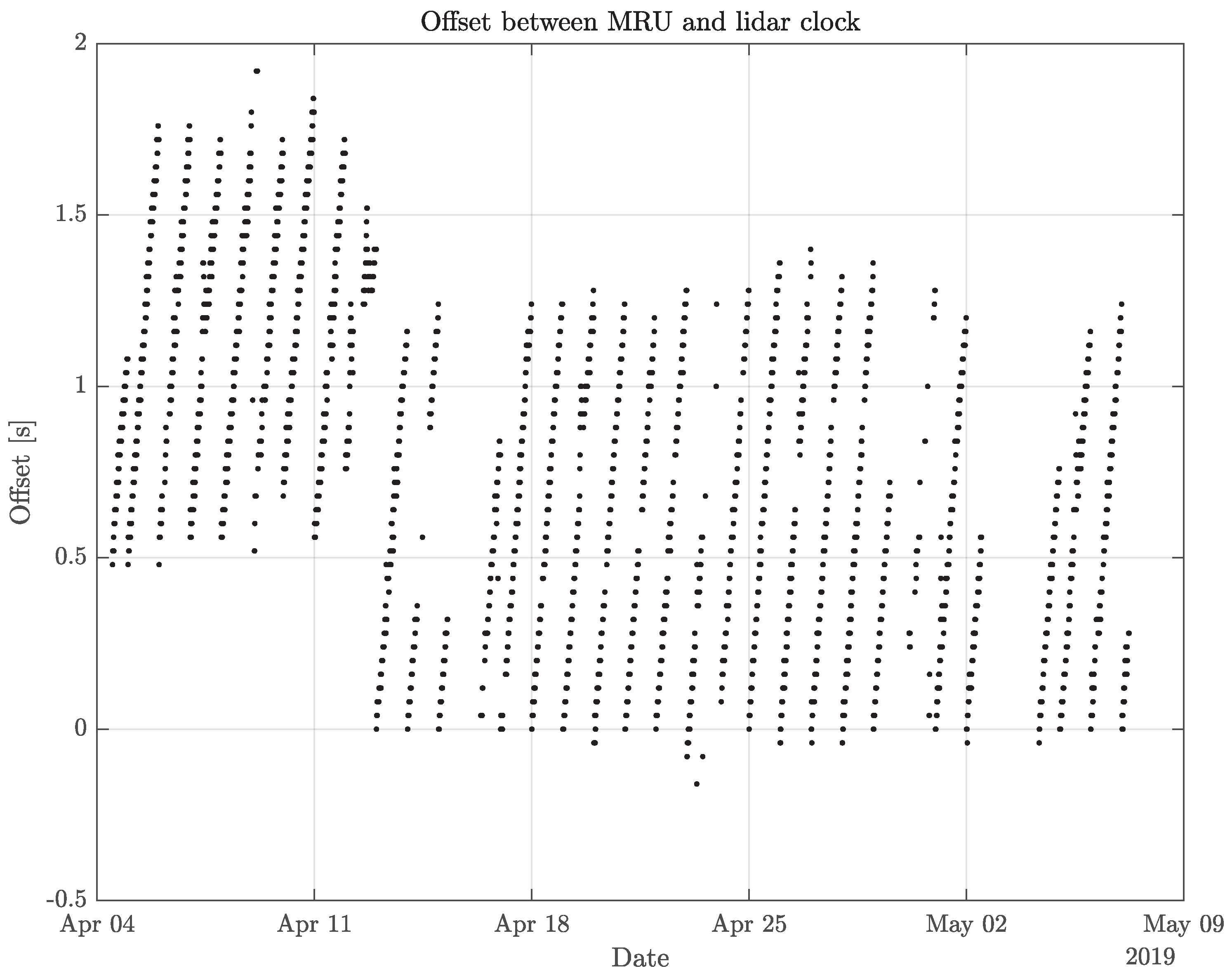
Figure 5 shows this sweet spot for all ten-minute intervals we processed for this study. We see the drift of approximately before the custom lidar timestamp is reset once per day, as described earlier in this section. The drift seems to occur linearly, and a sweet spot is found for all intervals.
Figure 5.
Timing offset at which the sweet spot from Figure 4 is found for all available ten-minute intervals.
3.4. Data Handling
After applying the motion compensation algorithm, we have three different sets of horizontal wind speed time series from the floating lidar. Of all three time series, we estimate according to Equation (4). These are from the internally-processed uncompensated values as they are stored in the 1 files, the values based on the emulated processing described in Section 3.1, and from the motion-compensated time series. As shown in Figure 3, and are not identical. In order to get motion-compensated turbulence estimates from the floating unit that are comparable to the internally-processed values of a fixed reference unit, we define the motion-compensated turbulence intensities as
Effectively, the amount of motion-induced turbulence is deducted from the uncompensated internally processed values to get compensated values that are comparable to a reference lidar with the same internal data processing.
3.5. Instrumentation and Measurement Setup
In order to validate the performance of the motion compensation algorithm, we compare measurements of the floating lidar with data from a fixed reference lidar. The validation campaign took place between 04.04.2019 and 07.05.2019 close to Titran on the Norwegian island of Frøya.
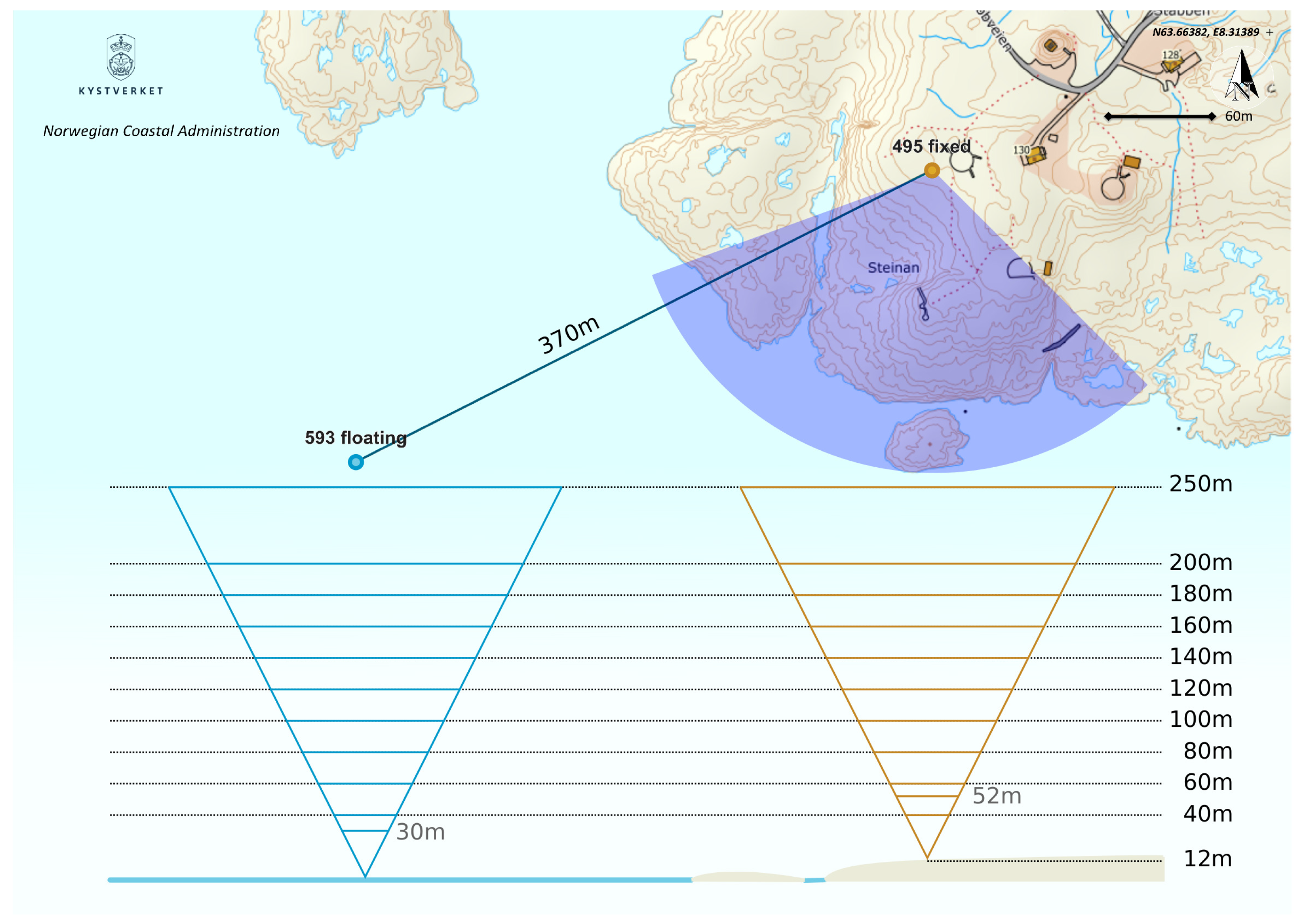
The floating lidar system is a ZX300M (unit 593, filter version 1.061) by ZX Lidars (Ledbury, United Kingdom) which is a vertical profiling, continuous-wave wind lidar. It is mounted on a SEAWATCH Wind LiDAR Buoy by Fugro (Leidschendam, Netherlands). The buoy is equipped with an MRU 6000 motion reference unit by Norwegian Subsea (Oslo, Norway) that measures the motion of the buoy in all six degrees of freedom with an update frequency of . For land-based reference measurements, a fixed ZX300 (unit 495, filter version 1.061) operating nearby onshore was used. The location of both lidars is marked on the map in Figure 6.
Figure 6.
Map indicating the location of the floating lidar unit 593 and the land-based fixed reference lidar unit 495. The elevation difference above sea level and the geometry of the measurement cones is shown for all measurement heights. The selected offshore wind sector is indicated in dark blue. (Map data adapted from www.kartverket.no).
Both lidar units are configured to measure the wind velocities at eleven heights, including the fixed reference height of above ground. The ground elevation at the location of the land-based reference lidar is above the mean sea level, and the window height is above the ground. The floating lidar is located at sea level and its window height is above sea level. The measurement heights are selected so that both lidars measure at ten identical elevations between and above sea level, as shown in Figure 6. Validation tests such as described in Mark et al. [26] support the assumption that lidar measurements with this setup are comparable for horizontal mean wind speed and wind direction. Due to the higher elevation of the fixed reference lidar compared to the floating lidar, its focus distances are slightly shorter for the same measurement height above sea level. This results in reduced line-of-sight averaging and also a reduced diameter of the measurement cone. The internal estimation of the ZX300 uses an empirical correction factor to make the lidar derived values more comparable to values from cup anemometers [27]. This correction factor is a function of measurement height and lidar measured . We do not apply this correction factor to our estimates but we can use it to get an approximate idea of the impact of the reduced line-of-sight averaging and reduced diameter of the measurement cone of the fixed reference lidar. We can take the average value of that we measured with the fixed reference lidar during the measurement period. The mean correction factor for all measurement heights is then higher for measurements taken at higher elevations. From this we can conclude that we expect the floating lidar to measure approximately less turbulence intensity at comparable heights due to its longer focus length. This is the only information we use the correction factor for in this study. All results shown in Section 4 of this paper are presented without application of the correction factor.
To make a meaningful comparison of turbulence measurements at the two locations, it is important to choose inflow wind directions in which the surface roughness is identical for both lidars. Thus, we decided to include data from the southern offshore sector with the limits and , as shown in Figure 6. In this sector, no land is present within a radius of . Because this stretch of undisturbed inflow is long compared to the distance between the two lidar units, we assume that both devices see approximately the same turbulence.
3.6. Data Filtering
The measurement campaign consists of 4860 ten-minute intervals. However, as seen in Figure 5, some data are missing due to irregularities in the required manual raw-data streaming, so only 4284 ten-minute intervals of raw data are available from the floating lidar. Before computations start, we exclude intervals where for at least one height level the output in the ten-minute files is flagged with either 9998 or 9999. These intervals are usually characterized by fog, very clear air with not enough backscatter, or very low wind speeds. We also exclude intervals during which at least at one height the measured mean wind velocity is below , since they are of low relevance for wind power and the wind vector reconstruction might be less accurate. Starting a new raw data file during one ten-minute interval causes the raw data to be split into two files. We do not merge them but filter out files for which less than of the raw dataset is available. After this initial filtering, 3863 intervals remain for data processing.
During processing of the remaining files, we check the internally-processed wind data files for 9998 and 9999 flags and filter out each reconstructed wind vector which is flagged by the lidar software. We also filter out all intervals for which the fixed reference lidar outputs a 9998 or 9999 mean value for at least one height level. This keeps all intervals for which data are available from all height levels from both lidar units. We then filter for inflow from the offshore sector , leaving us with a total of 889 intervals for comparison. Table 1 gives an overview of the wind conditions and the motion states of the buoy during the observation periods that are included in the comparison after filtering.
Table 1.
Overview of wind conditions and motion state of the buoy during the periods that are included in the results section. Wind conditions as measured by the fixed reference lidar.
3.7. Measurement Uncertainty
We know of several sources of error that might lead to uncertainties in our results. During the process of synchronizing the MRU and lidar data, we choose a time step of in order to find a good compromise between precision and computation time. For that reason, we expect that the sweet spots shown in Figure 5 are on average away from the correct values. In Figure 4 we see that the resulting error has approximately a cosine shape with an average period of . We therefore expect only a small statistical error of of the motion-induced due to this timing error.
The manufacturer of the MRU has indicated an accuracy of the roll and pitch angle measurements of . Considering that the mean tilt angle is approximately two orders of magnitude higher, we assume that the measurement error due to wrong tilt angles is below of the rotation-induced . The yaw angle error of the MRU is . A similar uncertainty should be expected from the alignment between the lidar beam direction and the x-direction of the MRU. Both can result in increased directional inaccuracy, which is not the object of investigation here. Uncertainties in surge and sway velocities are unfortunately not specified by the manufacturer, but results from a hexapod test with a JONSWAP motion spectrum with a peak period of and a significant amplitude of show a velocity error of . Velocities in the heave direction are expected to have a smaller error due to the well-defined zero baseline, which corresponds to an error of up to of the induced by translation at a horizontal mean wind speed of . We can conclude that the accuracy of the MRU is well-suited to the task, and we expect less than combined systematic error due to timing and precision of the motion measurement.
Strong statistical uncertainty arises from the test setup with two lidars measuring at two locations separated by . In most cases, the mean wind direction is not aligned with the separation distance. We assume that the wind vectors at both locations are independent. In addition, the lidars do not sample the wind continuously. Measurement at eleven height levels plus the time required to refocus the laser beam result in on average only samples for each height during one ten-minute interval. In the results (Section 4.5), we will quantify the statistical error of this slow sampling of independent wind vectors with lidar devices to approximately of the measured . We must therefore assume that even if the motion compensation algorithm were to work perfectly, a high amount of scatter would be found between the values measured by the fixed land reference lidar and the motion-compensated floating lidar.
4. Results and Discussion
4.1. Mean Wind
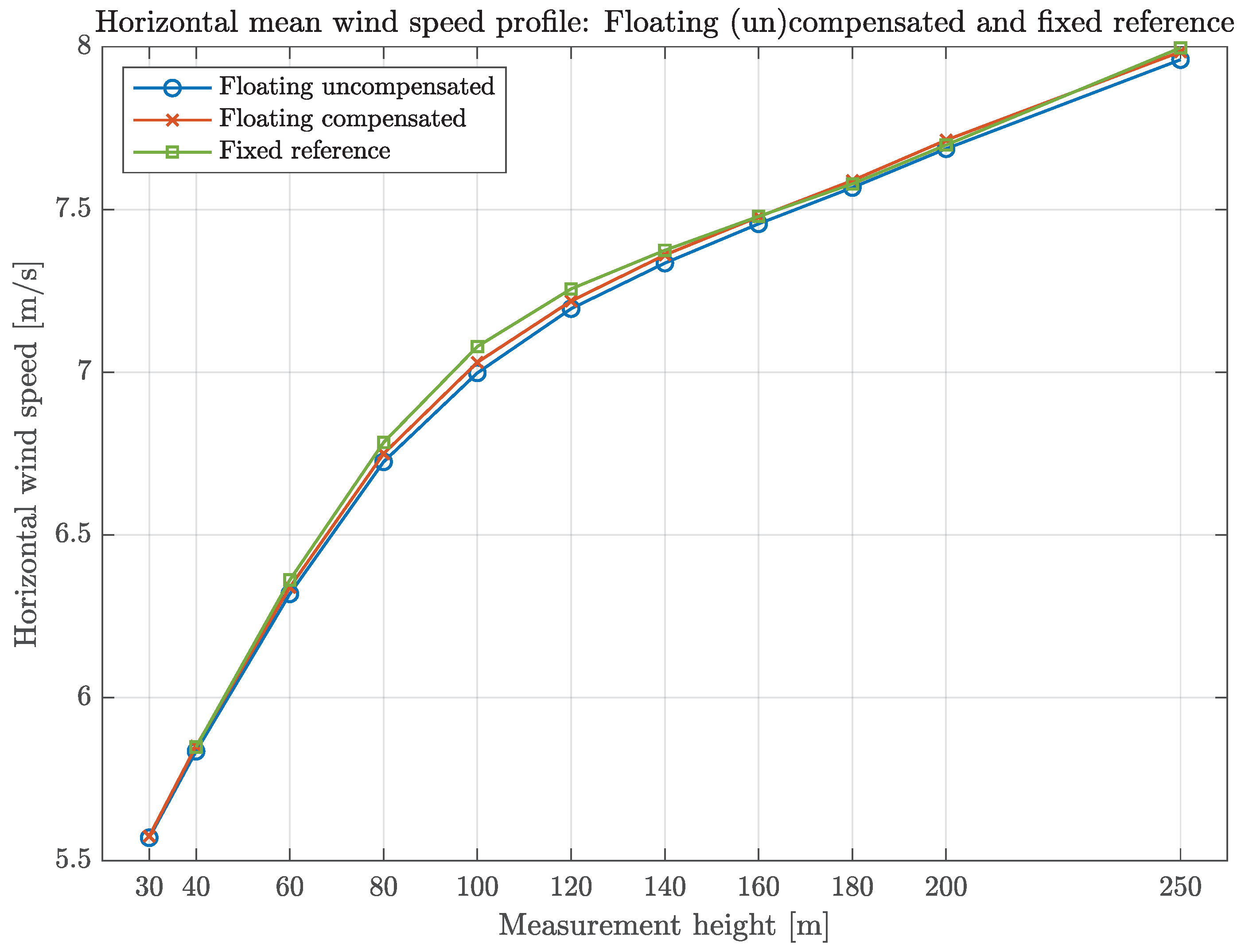
Correct measurements of the mean wind velocity are an essential prerequisite for valid estimates of . We therefore refer to Figure 7 which shows the average horizontal mean wind speeds for all intervals included by measurement height. The mean wind speed of all measurements included in the data comparison is . The floating lidar measures on average percent lower wind velocities. When motion compensation is applied, the error is reduced to . Most of this deviation is found in measurements at elevations between and . It is difficult to say if the real wind speed is absolutely identical at all elevations at both measurement locations. It is possible that the small change in ground elevation between the two lidar units leads to a small speed up or the increased surface roughness results in slowing the wind down slightly. Overall we conclude that the two measurement locations are comparable in terms of horizontal mean wind velocity, as previously reported [26], and that the motion compensation algorithm has a small influence that appears to improve the mean wind velocities.
Figure 7.
Average of measured horizontal mean wind velocities from the floating lidar with (red) and without (blue) motion compensation, as well as from the fixed reference lidar (green), sorted by measurement height.
4.2. TI Profile
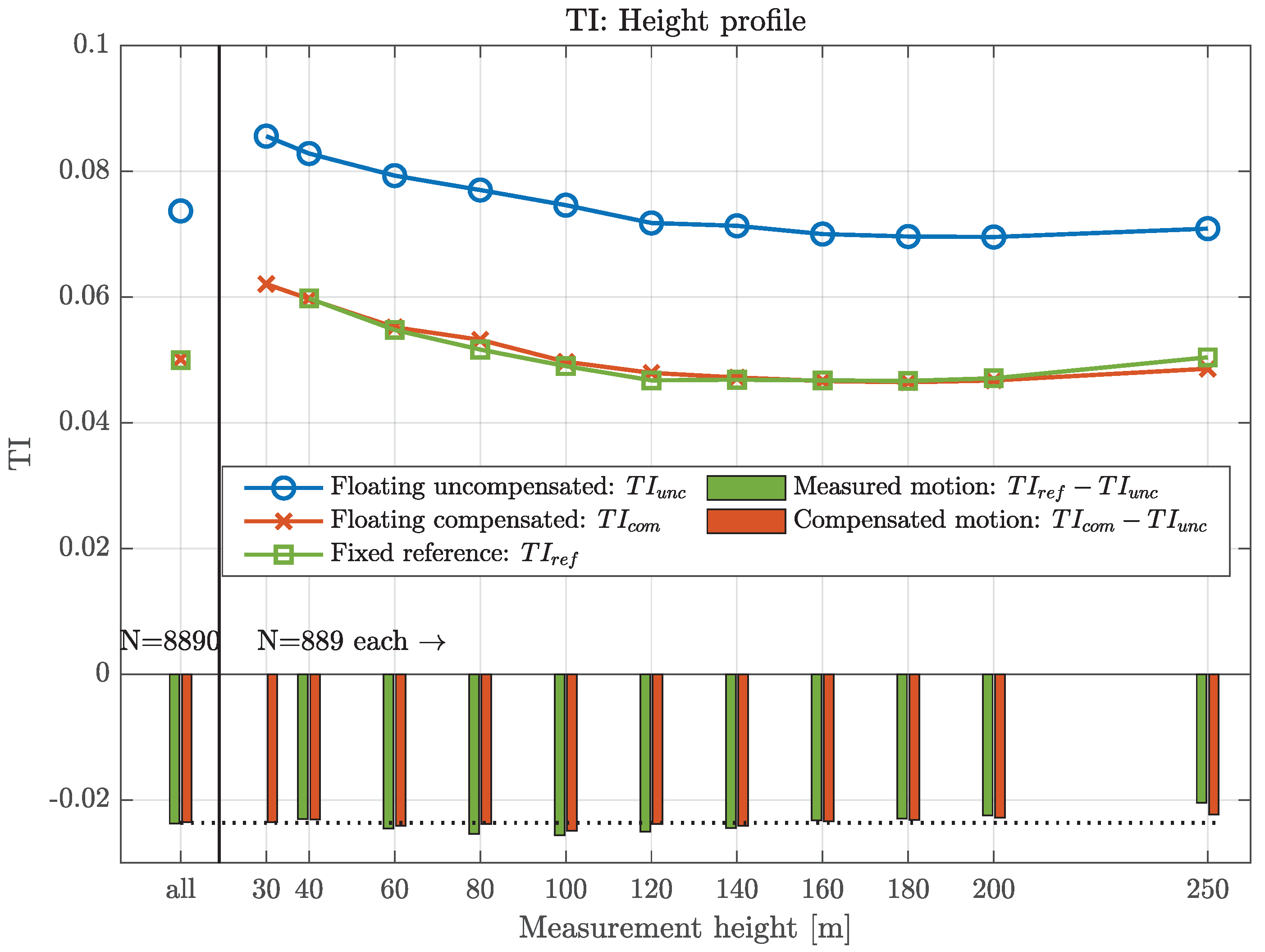
Figure 8 shows that the reference lidar measures an average value of across all test intervals. This value might seem low when compared with other offshore wind data. However, the ZX lidar correction factor of, in this case, that we did not include in our results would lift the values to what we would expect from an offshore site [28]. Looking at at different height levels, we observe a characteristic profile with higher turbulence close to the ground, which creates turbulence from uniform shear. decreases for increasing height and reaches its minimum at around . For the highest elevation at , measured increases again slightly. Such a behavior has been reported by Svensson et al. [29]. We think this could be due to lower Doppler signal quality at high elevations that lead to an increased standard error of the wind vectors and thus higher estimates.
Figure 8.
Average for all measurements and sorted by measurement heights. Blue circle markers indicate based on uncompensated measurements from the floating lidar. Red cross markers show corresponding values with motion compensation. Green square markers stand for values from the land-based fixed reference lidar for comparison. Bar plots show the motion-induced as the difference between measurements with the floating lidar and the fixed lidar (green) compared to the amount of motion-induced detected by the algorithm (red). The number of available measurement values at each height is given.
The floating lidar without any compensation measures a mean . The shape of the profile is similar to the reference profile, but all values are on average approximately higher due to motion-induced turbulence. The motion compensation reduces the estimates to a level of , which is very close to the reference value and equals a motion reduction factor of 99.8%. Overall, the profile follows the profile. The bar plots in Figure 8 visualize the amount of motion-induced in two ways: first, we present the difference between the uncompensated floating and fixed measurements (green); second, we show the amount of motion-induced detected by the algorithm (red), which is the difference between uncompensated floating and compensated floating . Each pair of bars would have the same length if the motion compensation algorithm were perfect and the measurements from both locations were fully comparable.
We will now analyze the motion-induced at all but the highest elevation, which we will analyze later. The lengths of all bars representing measured motion-induced at heights from to lie in a narrow band of around the mean of all heights marked by the horizontal dotted line. The measured motion-induced values show above-average values from to . These height levels coincide with where we measured lower values of mean wind speed from the floating lidar (see Figure 7). We can show that the lower mean wind speed is responsible for approximately half of the deviations from the mean measured motion-induced . With this correction in mind, we can say that motion-induced is only weakly dependent on measurement height, with a slight tendency towards lower values at high elevations. This suggests that rotational motion, as described in Section 2.3.2, is dominant compared to the contribution of translational motion described in Section 2.3.1. Rotational motion contributes velocity variance proportional to the mean wind speed. Because values are normalized by the mean wind speed, the influence of rotation on the results has to be identical at all measurement heights. By contrast, translational motion introduces an identical amount of velocity variance at all heights, which results in lower motion-induced values at greater heights, where the mean wind speed is faster. The effect of wind shear and veer described in Section 2.3.3 can be different at each height, but we consider it to be of minor importance.
The motion-induced detected by our algorithm is very similar to the measured values, especially when the remaining differences in mean wind speed from to are taken into consideration.
As mentioned before, the fixed reference lidar measures slightly higher at its highest measurement level, , which could be caused by weak backscatter signal quality at this elevation. The floating lidar shows the same effect but to a smaller extent. It seems that although both lidars are of the same type, the error caused by low backscatter at the highest elevation affects the reference lidar more than the floating lidar. This would explain why the measured, motion-induced is erroneously low compared to the value our algorithm calculates. If this explanation is correct, the overall measured by the reference lidar is a bit higher than what we measure with a perfectly motion-compensated floating lidar. Additionally, the shorter focus lengths and reduced measurement cone diameters lead to slightly increased values from the reference lidar, as shown with the help of the correction factor in Section 3.5. In this case, both effects combined seem to outweigh the imperfections of the motion compensation nearly exactly, which explains the overall performance of the motion compensation algorithm.
4.3. TI vs. Velocity
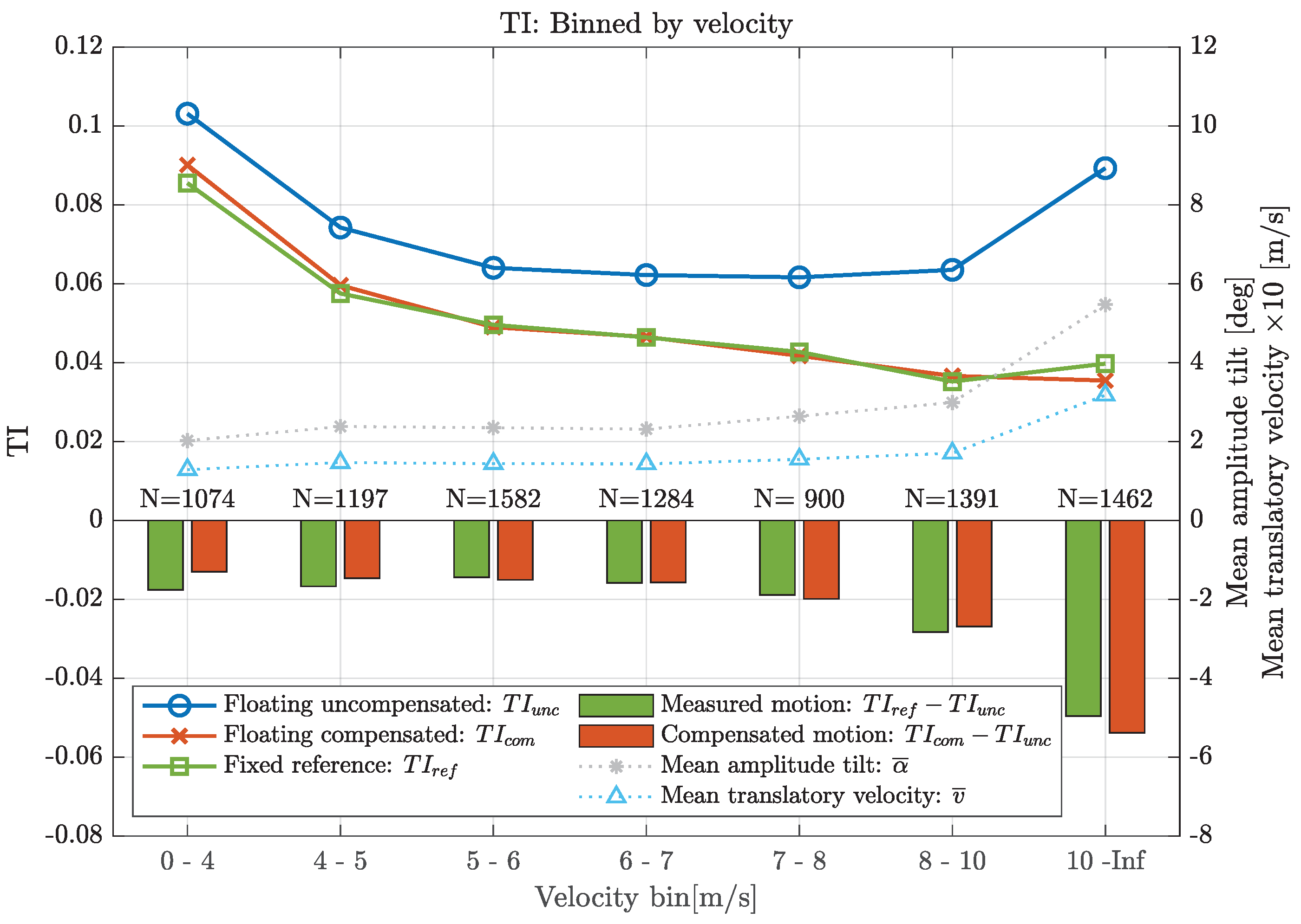
In order to find out if the motion compensation algorithm works similarly well under the influence of varying mean wind conditions, we look at Figure 9. The estimates measured by the land-based reference lidar gradually decrease with increasing wind velocity. At the lowest wind speeds, the turbulence is dominated by thermal effects that do not increase with wind speed proportionally [15]. therefore decreases at increasing wind speeds. However, for the strongest wind speed bin, is slightly higher again, which can be explained by the increased surface roughness of the wavy sea [28]. The increasingly rough sea state at increasing wind speeds is represented in the figure by the gray and blue markers that indicate the measured mean tilt amplitude and mean velocity of the buoy, respectively.
Figure 9.
from all measurement heights binned by mean wind velocity. Legend as in Figure 8 plus markers for the mean tilt amplitude and mean translational velocity that scale with the right hand side y-axis.
The floating lidar shows higher values. We see that at low wind speeds the measured motion-induced is slightly higher than at intermediate wind speeds between and , although the motion parameters tilt amplitude and translational velocity are the lowest. The reason is probably that the translational motion is more important for the total motion-induced at very low wind speeds. As an example, we can imagine two cases in which the amounts of translational and rotational motion are identical but the mean wind speed is different. The identical amount of translational motion leads to the same amount of measured velocity variance but higher motion-induced in the low wind speed case. The identical amount of rotational motion leads to an increase in velocity variance that is dependent on the wind velocity, and therefore leads to the same amount of motion-induced . Taken together, motion-induced is higher for the low wind speed case. In our lowest wind speed case, the amount of motion is lower than for higher wind speeds, but it is not as low as it would need to be to compensate for the effect we just sketched out. At higher wind speeds above motion-induced, increases with wind speed due to the dominance of the effect of rotational motion.
When the of the land reference lidar is now compared to the motion-compensated of the floating lidar, we see overall good agreement, which means that the motion compensation algorithm is able to correct for motion under all tested wind conditions. The strongest deviation is found for the lowest wind velocities, where the actual reduction is underestimated by the motion compensation algorithm. The reason could lie in how we assign a sign to the radial velocities. As described in Section 3.2, the risk of assigning the wrong sign is higher for low wind speeds. With the wrong sign assigned to some radial velocities, the motion compensation does not work correctly. This could explain why we under-compensate the motion during low wind phases. Further investigation, e.g., with in-situ anemometry, is required to test this explanation.
At high wind speeds above the algorithm slightly overestimates the amount of motion-induced . Such high mean wind speeds appear jointly with high tilt amplitudes. In the next subsection we provide a detailed analysis of this error.
4.4. TI vs. Tilt Angle
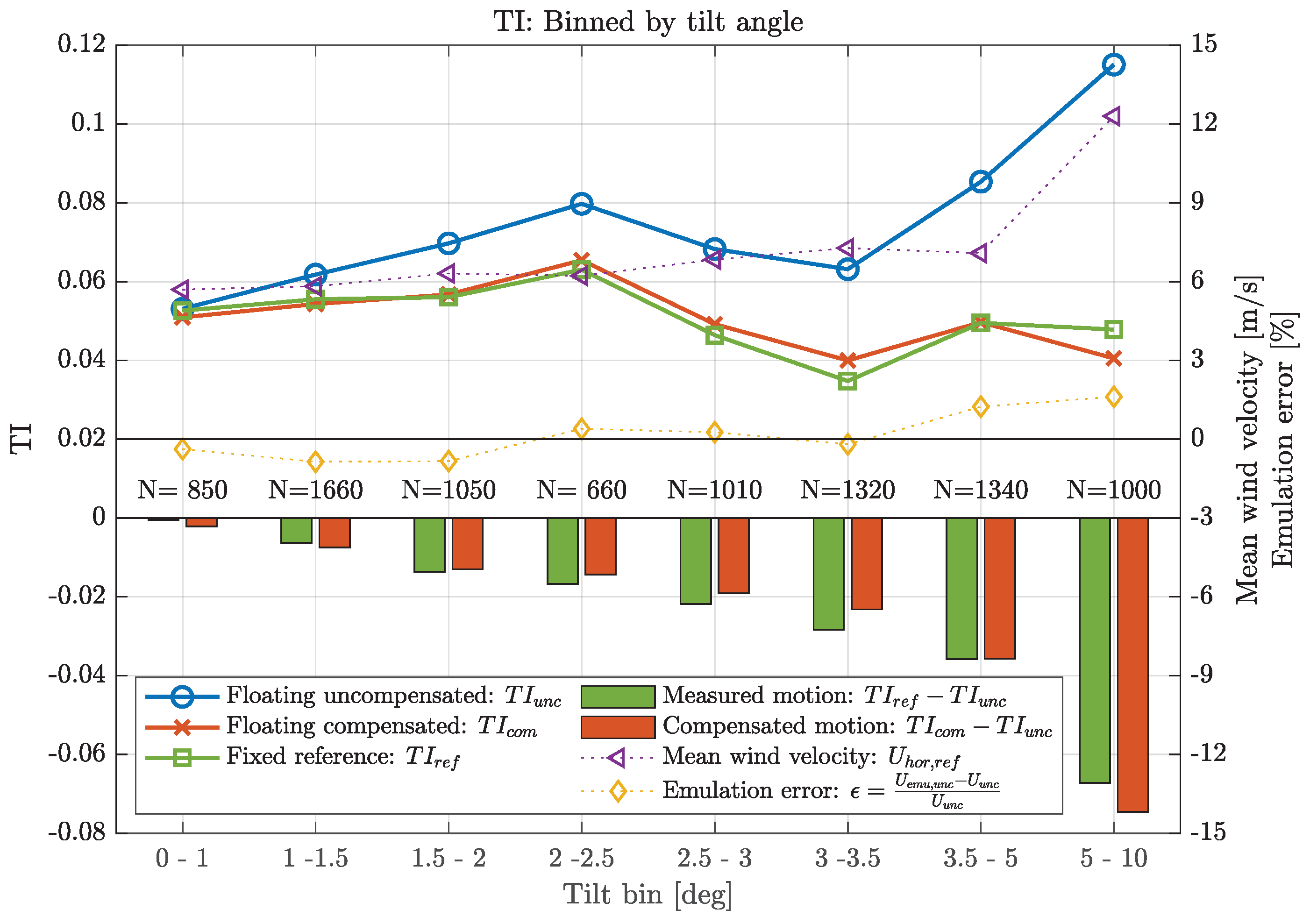
Figure 10 shows the values binned by mean tilt angles. measured by the land-based reference lidar lies between and . Low tilt angles are correlated with high values via low wind speeds. High tilt angles are also correlated with high values via rough sea states. It is therefore not surprising that we do not see a systematic trend in the fixed reference lidar measurements.
Figure 10.
from all measurement heights binned by , the mean tilt angle of the buoy. Legend as in Figure 8 plus markers for the horizontal mean wind velocity U and the relative emulation error that refer to the right hand side y-axis.
The floating lidar overestimates . The extent of this overestimation is strongly dependent on the tilt amplitude. Strong motion leads to measurements of high motion-induced . When the mean tilt amplitude is below , the measured motion-induced is only , which seems unrealistically low in comparison to the value of measured for . The reason could be that the reference lidar always measures slightly higher amounts of compared to the floating lidar due to its elevated location and lower measurement height above the ground.
Moreover, the motion compensation algorithm shows steadily increasing motion-induced turbulence intensities for increasing tilt angles. However, while it slightly underestimates the real conditions in most cases, an overestimation of the motion-induced turbulence is found at high tilt angles . We suspect that deviations between the lidar’s internal data processing and the results of our emulated processing correlate with the overestimation of motion-induced . We therefore included the relative deviation of the mean wind speeds from internal processing and emulated processing into Figure 10 and see that the highest emulation error coincides with the overestimation of motion-induced at high tilt amplitudes. A high emulation error is probably due to the presence of clouds or fog that are handled differently by internal and emulated data processing. Nearly all of the 100 intervals in the high tilt bin are shown in the strong motion example given in Figure 11, which we will analyze next.
Figure 11.
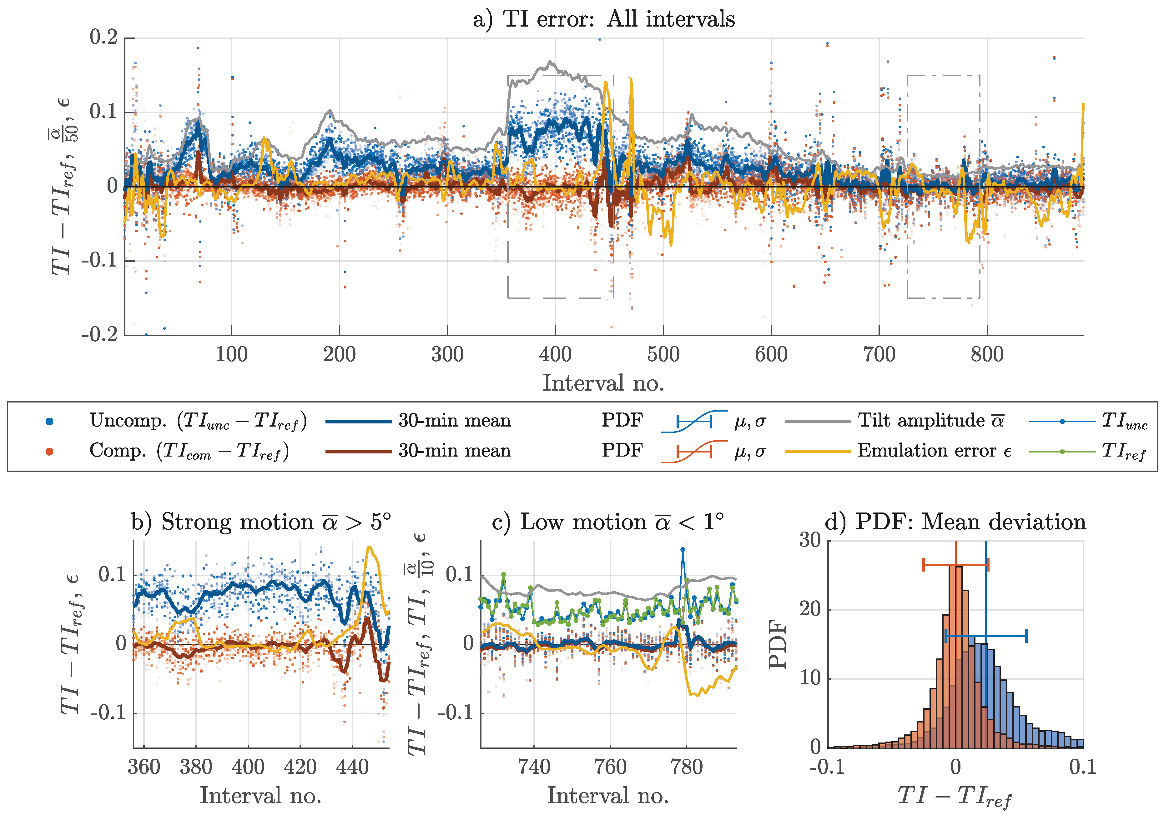
Top: (a) Overview of the individual error between measured by reference lidar and uncompensated floating lidar (blue) and compensated floating lidar (red). Bottom: Close up view of two examples of the plot above where the motion-induced turbulence is particularly high (b) and low (c). (d) Probability density functions (PDF) of the error
4.5. Individual Error Analysis
All 889 intervals that contain measurements of 10 comparable height levels are shown in Figure 11a. The figure depicts the difference between the values of the floating lidar and the fixed reference lidar. These differences are the measurement error of the floating lidar with regard to the fixed reference lidar. In accordance with the color scheme used for the profiles in Figure 8, Figure 9 and Figure 10, the errors of the uncompensated lidar are marked in blue, and the values of the compensated lidar are marked in red. The degree of transparency of each marker represents the measurement height at which the corresponding values are taken. Increasing transparency means increasing height. In addition to the individual values, the moving means over 30-minutes of data are also plotted. Positive values mean higher measured by the floating lidar. In gray, the mean tilt amplitude is also plotted, which is a good indicator of the error of the uncompensated floating lidar.
We see clearly that the biggest errors are found where the tilt angle is highest. Subfigure b to the left under the main plot zooms into this strong motion case with a mean tilt amplitude of . measured by the uncompensated floating lidar is much higher than the reference measurements for nearly all intervals. However, around intervals 375, 422, and 437, they drop significantly, and at interval 452, the turbulence measured by the floating lidar without any compensation is even lower than the measurements from the fixed reference. This is even more surprising when considering that the mean tilt amplitude during these intervals is always . We must therefore assume severe measurement issues in one or both of the lidars. This assumption is supported by finding high emulation errors at the same time intervals. This emulation error marked in yellow is, as explained before, an indirect measure of the amount of filtering or cloud detection in the internal data processing of the floating lidar. The values of motion-compensated in the proximity of these four intervals (375, 422, 437, and 452) are on average below the reference line. We remember from Figure 10 that the strong wind case which we look at here is characterized by overcompensated motion. But now it appears that the error does not lie in the motion compensation but might already be contained in the turbulence measurements of one or both of the lidar units. To strengthen this hypothesis, we now look at the test cases with low motion where , shown in detail in the next subfigure.
The intervals in Figure 11c are in general characterized by a low error between floating and fixed lidar measurements visible by the floating mean lines fluctuating around zero. The effect of applied motion compensation is so low that both lines often overlap, which is reasonable, since the mean tilt amplitude is always very low with an average value of . Around interval 779 the error suddenly jumps to for both the uncompensated and the compensated cases, which have nearly identical values. The cause of this significant error becomes clear when the 10-min mean values of of the fixed reference lidar (green lines) are compared with the of the uncompensated floating lidar (blue lines with markers). During interval 779, the floating lidar measures much stronger values than the reference lidar. We think that the discrepancy between these two measurements cannot be caused by the very low motion of the floating lidar. Instead, we assume that it is caused by poor signal quality of the floating lidar in this particular situation. We cannot test this hypothesis, but it is supported by the high level of activity of the filter in the floating unit just before and after the suspicious interval.
The low motion case can be used for a second purpose, which is the approximate estimation of the scatter resulting from measurements with two lidars at two different locations that take a low number of samples per ten-minute interval (). The average measured by the reference lidar during the low motion case is . The turbulence conditions are thus representative of the complete studied dataset (). The motion-induced for the low motion case according to the motion compensation algorithm is just . This value is so low that we now assume that the uncompensated measurements from the floating lidar during the low motion case are comparable to measurements from a fixed lidar. The error we find between the floating lidar and the fixed reference must therefore be caused by the measurement setup. We calculate the standard error of the uncompensated samples in the low motion case to be . This means the statistical error involved in sampling independent wind vectors with two lidar devices and only 37 measurements per ten minutes is of the measured . Expressed differently, this means that of the total standard error we find in the compensated data for the entire campaign () is caused by the measurement setup.
The histogram plotted in Figure 11d shows the probability density function of all individual samples of the error between floating and reference lidar for uncompensated (blue) and compensated (red) measurement data. While the uncompensated values show a bias of and a standard deviation of , the compensated values show a bias of only and a standard deviation of . Uncompensated values have a positive skewness of . The motion compensation reduces this positive skewness and results in . The remaining skewness can be explained by the possibility for values to theoretically be infinitely high but not negative. This limitation explains the skewness, which means that high positive error values are more likely than high negative error values.
The analysis of the error leads to the conclusion that the biggest errors found between the motion-compensated values from the floating lidar, and the values from the reference lidar are likely not caused by an insufficiency of the motion compensation but rather by measuring with two different units at two different locations. A longer dataset would probably mitigate the resulting effect on statistical profiles like Figure 9 and Figure 10.
4.6. Scatter Analysis
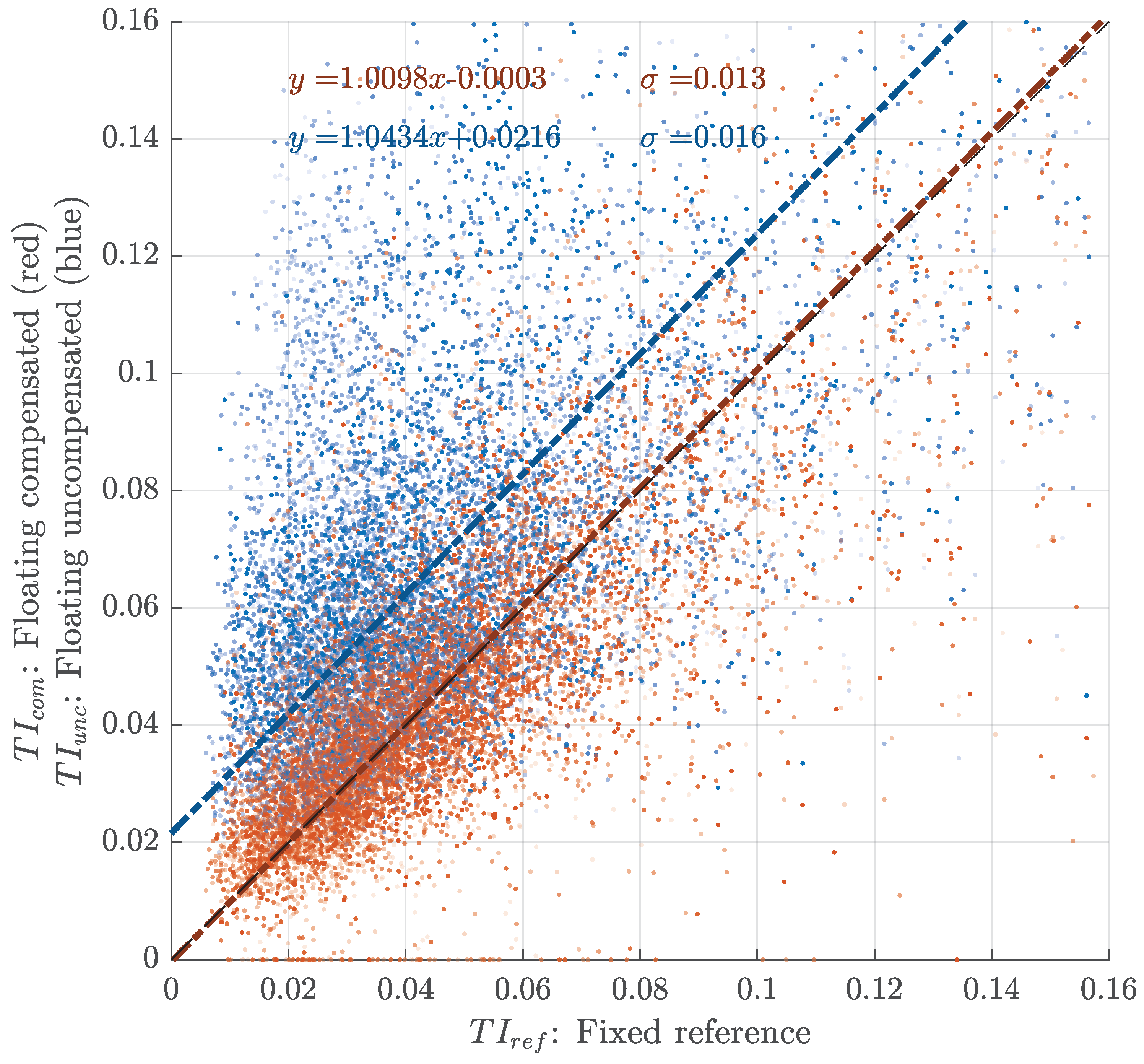
Figure 12 shows a scatter plot of the results. For each single measurement from each measurement height, we plot the value of the floating lidar on the y-axis and the value of the fixed reference lidar on the x-axis. The uncompensated data pairs are, as before, marked in blue, while the results after compensation are shown in red. Additionally, here, the degree of transparency of each marker represents the measurement height. Because all three datasets were acquired using the same lidar measurement technology, we can assume that the reference values from the fixed land-based lidar have significant uncertainty as high as the uncertainty of the floating lidar with perfect motion compensation. We therefore decided to add Deming regression lines with according to Adcock [30] that are characterized by having minimized squared perpendicular distances from the data points. This orthogonal regression avoids the positive offset and slope found when conventional linear regression is applied to data with similar uncertainty for x and y values [31]. Data pairs from a perfectly motion-compensated and a fixed lidar would be scattered around the diagonal line (black dashed line). It is apparent also from the scatter plots that the uncompensated estimates of the floating lidar are too high, as most blue markers lie above the line. This overestimation of or positive turbulence intensity error appears to be nearly constant across the entire range of turbulence intensities contained in the dataset. The blue regression line shows an offset of for very low turbulence cases. With its slope of , it reaches an error of for where the data density is too low for statistically relevant conclusions. The standard error of the regression line is .
Figure 12.
Scatter plot of turbulence intensities from the floating lidar uncompensated (blue) and compensated (red) vs. from the land-based reference lidar. Deming regression lines are given in corresponding colors. The equations of the regression lines and their standard deviations are listed. The black dashed line is the line. Some datapoints lie outside the plotted area.
The red markers representing the compensated floating lidar results versus the reference lidar also show high scatter of , which is nearly centered around the line. The determined offset at the origin is only and the slope of leads to an error of motion-induced turbulence of for cases with . Due to the minimization of the quadratic distances, the influence of data points with high scatter is overrepresented in the calculation of the regression lines. But a repeated analysis that excluded all values showed a regression line with a slope of , an offset of , and . These values predicted by the linear regression model are very good.
5. Conclusions
We show that estimates of measured by a floating VAD scanning continuous-wave wind lidar are comparable to those of a fixed land-based reference lidar of the same type when implementing an algorithm to compensate for the motion of the floating lidar at the line-of-sight level in all six degrees of freedom. A comparison of mean values of shows good agreement between motion-compensated measurements from a floating lidar and a fixed reference lidar for a wide range of mean wind speeds and buoy tilt angles. Strong scatter caused by the low sampling rate of the reconstructed wind vectors at each measurement height is present in the results due to the high number of scanned elevation levels (eleven), which results in a low number of samples per ten-minute interval. Additionally, the relatively wide spatial separation between the floating lidar and the land-based reference lidar () increases the expected amount of scatter. All reported values are lidar-measured. We expect them to deviate from the real values and in this study do not try to assess or improve the capability of profiling wind lidars to measure turbulence.
Successful motion compensation requires reliable time synchronization between motion data and lidar data. We achieved this by computing the motion compensation within a range of time lags and selecting the offset that results in the strongest reduction in measured wind velocity variance. A more native solution, e.g., by increasing the resolution of the timestamp information of the lidar, would be desirable. The method presented in this study requires access to the line-of-sight wind velocity estimates of the ZX300 wind lidar. We therefore saved Doppler spectra measured by the unit on a connected PC. This prevents the presented method from being applied on existing ZX300 data without stored line-of-sight data. To determine the line-of-sight velocities from the Doppler spectra, we employ a simple centroid method which deviates from the internal data processing that we do not have access to. To still get reliable motion-compensated turbulence information, we subtract the motion-induced calculated by our own processing from the values estimated by the lidar’s internal data processing. It would be advantageous if the internally processed line-of-sight velocities were available for motion compensation by default, as is the case for example for the Windcube by Leosphere (Saclay, France). Moreover, the availability of signed line-of-sight velocities would help to improve the accuracy of motion compensation. Suggestions on how to determine the direction of the radial velocities measured by continuous-wave wind lidars can be found in [32,33].
Further research should analyze measurements of a floating and a closely collocated fixed lidar that simultaneously measure at only one height level. Such a setup would result in much smaller statistical error and would perhaps make a time series comparison useful. Applying the method presented here to a Doppler beam swinging wind lidar, such as the Windcube, could be a different option for further work. This lidar type outputs its internally processed line-of-sight velocities by default, but the accumulation time spent in each beam direction must to be considered when processing motion data.
Author Contributions
conceptualization, F.K.; data curation, F.K.; formal analysis, F.K.; funding acquisition, V.N. and L.L.; investigation, V.N. and L.L.; methodology, F.K.; project administration, V.N. and L.L.; software, F.K.; supervision, T.B. and J.M.; visualization, F.K.; writing—original draft, F.K.; writing—review and editing, F.K., T.B., and J.M. All authors have read and agreed to the published version of the manuscript.
Funding
The Norwegian Public Roads Administration (Statens vegvesen) as part of the project “Metocean Data for Large Fjord Crossings on the E39” funded the SEAWATCH Wind LiDAR Buoy, including its measurement instrumentation. The presented work is part of a PhD project funded by Energy and Sensor Systems (ENERSENSE) at the Norwegian University of Science and Technology. The APC was funded by NTNU’s Publishing Fund.
Acknowledgments
We acknowledge the work of Kam Sripada, who proofread the manuscript.
Conflicts of Interest
The authors declare no conflict of interest. The funders had no role in the design of the study; in the collection, analyses, or interpretation of data; in the writing of the manuscript, or in the decision to publish the results.
Abbreviations
The following abbreviations are used in this article:
| LOS | Line-of-sight |
| MRU | Motion reference unit |
| NWU | North-west-up |
| Res. | Resonance |
| Rot. | Rotational |
| Std. dev. | Standard deviation |
| Turbulence intensity | |
| Transl. | Translational |
| VAD | Velocity–azimuth display |
References
- Petersen, S.; Sarmento, A.; Cândido, J.; Godreau, C. Preliminary study on an offshore wind energy resource monitoring system. In Renewable Energies Offshore; Soarez, C.G., Ed.; Taylor & Francis: Abingdon, UK, 2015; pp. 213–218. [Google Scholar]
- Gottschall, J.; Gribben, B.; Stein, D.; Würth, I. Floating lidar as an advanced offshore wind speed measurement technique: Current technology status and gap analysis in regard to full maturity. WIREs Energy Environ. 2017, 6. [Google Scholar] [CrossRef]
- The Carbon Trust. Carbon Trust Offshore Wind Accelerator Roadmap for the Commercial Acceptance of Floating LiDAR Technology. Version 2.0. October 2018. [Google Scholar]
- Tiana-Alsina, J.; Rocadenbosch, F.; Gutiérrez-Antuñano, M.A. Vertical azimuth display simulator for wind-Doppler lidar error assessment. In Proceedings of the 2017 IEEE International Geoscience and Remote Sensing Symposium (IGARSS), Fort Worth, TX, USA, 23–28 July 2017; pp. 1614–1617. [Google Scholar] [CrossRef]
- Gottschall, J.; Wolken-Möhlmann, G.; Viergutz, T.; Lange, B. Results and conclusions of a floating-lidar offshore test. Energy Procedia 2014, 53, 156–161. [Google Scholar] [CrossRef]
- Mathisen, J.P. Measurement of wind profile with a buoy mounted lidar. In Proceedings of the 10th Deep Sea Offshore Wind R&D Conference, DeepWind’2013, Trondheim, Norway, 24–25 January 2013. [Google Scholar]
- Gutiérrez-Antuñano, M.A.; Tiana-Alsina, J.; Salcedo, A.; Rocadenbosch, F. Estimation of the Motion-Induced-Horizontal-Wind-Speed Standard Deviation in an Offshore Doppler Lidar. Remote Sens. 2018, 10, 2037. [Google Scholar] [CrossRef]
- Tiana-Alsina, A.J.; Gutiérrez, M.A.; Würth, I.; Puigdefábregas, J.; Rocadenbosch, F. Motion compensation study for a floating Doppler wind LiDAR. In Proceedings of the 2015 IEEE International Geoscience and Remote Sensing Symposium (IGARSS), Milan, Italy, 26–31 July 2015. [Google Scholar] [CrossRef]
- Gutiérrez, M.A.; Tiana-Alsina, J.; Bischoff, O.; Cateura, J.; Rocadenbosch, F. Performance evaluation of a floating Doppler wind lidar buoy in mediterranean near-shore conditions. In Proceedings of the 2015 IEEE International Geoscience and Remote Sensing Symposium (IGARSS), Milan, Italy, 26–31 July 2015. [Google Scholar] [CrossRef]
- Yamaguchi, A.; Ishihara, T. A new motion compensation algorithm of floating lidar system for the assessment of turbulence intensity. J. Phys. Conf. Ser. 2016, 753. [Google Scholar] [CrossRef]
- Gottschall, J.; Wolken-Möhlmann, G.; Lange, B. About offshore resource assessment with floating lidars with special respect to turbulence and extreme events. J. Phys. Conf. Ser. 2014, 555. [Google Scholar] [CrossRef]
- Sathe, A.; Mann, J.; Gottschall, J.; Courtney, M.S. Can wind lidars measure turbulence? J. Atmos. Ocean. Tech. 2011, 853–868. [Google Scholar] [CrossRef]
- Kelberlau, F.; Mann, J. Better turbulence spectra from velocity-azimuth display scanning wind lidar. Atmos. Meas. Tech. 2019, 12, 1871–1888. [Google Scholar] [CrossRef]
- Kelberlau, F.; Mann, J. Cross-contamination effect on turbulence spectra from Doppler beam swinging wind lidar. Wind Energy Sci. Discuss. 2019. [Google Scholar] [CrossRef]
- Emeis, S. Wind Energy Meteorology, 2nd ed.; Springer International Publishing AG: Berlin/Heidelberg, Germany, 2018. [Google Scholar] [CrossRef]
- Grewal, M.S.; Weill, P.L.R.; Andrews, A.P. Global Positioning Systems, Inertial Navigation, and Integration; chapter Appendix C: Coordinate Transformations; John Wiley & Sons Inc.: Hoboken, NJ, USA, 2006; pp. 456–501. [Google Scholar] [CrossRef]
- Cole, I.R. Modelling CPV. Ph.D. Thesis, Loughborough University, Loughborough, UK, 2015. [Google Scholar]
- Gottschall, J.; Catalano, E.; Dörenkämper, M.; Witha, B. The NEWA Ferry Lidar Experiment: Measuring Mesoscale Winds in the Southern Baltic Sea. Remote Sens. 2018, 10, 1620. [Google Scholar] [CrossRef]
- Zhai, X.; Wu, S.; Liu, B.; Song, X.; Yin, J. Shipborne Wind Measurement and Motion-induced Error Correction of a Coherent Doppler Lidar over the Yellow Sea in 2014. Atmos. Meas. Tech. 2018, 11, 1313–1331. [Google Scholar] [CrossRef]
- Wolken-Möhlmann, G.; Lilov, H.; Lange, B. Simulation of Motion Induced Measurement Errors for Wind Measurements Using LIDAR on Floating Platforms; Fraunhofer IWES: Bremerhaven, Germany, 2010. [Google Scholar]
- Branlard, E.; Pedersen, A.T.; Mann, J.; Angelou, N.; Fischer, A.; Mikkelsen, T.; Harris, M.; Slinger, C.; Montes, B. Retrieving wind statistics from average spectrum of continuous-wave lidar. Atmos. Meas. Tech. 2013, 6, 1673–1683. [Google Scholar] [CrossRef]
- Angelou, N.; Foroughi Abari, F.; Mann, J.; Mikkelsen, T.; Sjöholm, M. Challenges in noise removal from Doppler spectra acquired by a continuous-wave lidar. In Proceedings of the 26th International Laser Radar Conference, Porto Heli, Greece, 25–29 June 2012. [Google Scholar]
- Pitter, M.; Slinger, C.; Harris, M. Introduction to continuous-wave Doppler lidar. In Remote Sensing for Wind Energy; DTU Wind Energy-E-Report-E-0084; DNV GL-Energy: Kaiser-Wilhelm-Koog, Germany, 2015. [Google Scholar]
- Mann, J.; Peña, A.; Bingöl, F.; Wagner, R.; Courtney, M.S. Lidar scanning of momentum flux in and above the surface layer. J. Atmos. Ocean. Technol. 2010, 27, 959–976. [Google Scholar] [CrossRef]
- Dellwik, E.; Mann, J.; Bingöl, F. Flow tilt angles near forest edges – Part 2: Lidar anemometry. Biogeosciences 2010, 7, 1759–1768. [Google Scholar] [CrossRef]
- Mark, A.; Köhne, V.; Stein, D. Assessment of the Fugro OCEANOR Seawatch Wind LiDAR Buoy WS 170 Pre-Deployment Validation at Frøya, Norway; Technical Report GLGH-4270 17 14462-R-0002, Rev. C; DNV GL-Energy: Kaiser-Wilhelm-Koog, Germany, 2017. [Google Scholar]
- Wylie, S. Turbulence Intensity measurements from a ground-based vertically-profiling lidar. In Proceedings of the WindEurope Resource Assessment Workshop Session 4: Using Lidar to Reduce Uncertainty, Brussels, Belgium, 27–28 June 2019. [Google Scholar]
- Türk, M.; Emeis, S. The dependence of offshore turbulence intensity on wind speed. J. Wind Eng. Ind. Aerodyn. 2010, 98, 466–471. [Google Scholar] [CrossRef]
- Svensson, N.; Arnqvist, J.; Bergström, H.; Rutgersson, A.; Sahlée, E. Measurements and Modelling of Offshore Wind Profiles in a Semi-Enclosed Sea. Atmosphere 2019, 10, 194. [Google Scholar] [CrossRef]
- Adcock, R.J. A Problem in Least Squares. Analyst 1878, 5, 53–54. [Google Scholar] [CrossRef]
- Cornbleet, P.J.; Gochman, N. Incorrect least-squares regression coefficients in method-comparison analysis. Clin. Chem. 1979, 25, 432–438. [Google Scholar] [CrossRef] [PubMed]
- Abari, C.F.; Pedersen, A.T.; Mann, J. An all-fiber image-reject homodyne coherent Doppler wind lidar. Opt. Express 2014, 22, 25880–25894. [Google Scholar] [CrossRef] [PubMed]
- Gao, S.; Hui, R. Frequency-modulated continuous-wave lidar using I\Q modulator for simplified heterodyne detection. Opt. Lett. 2012, 37, 2022–2024. [Google Scholar] [CrossRef] [PubMed]
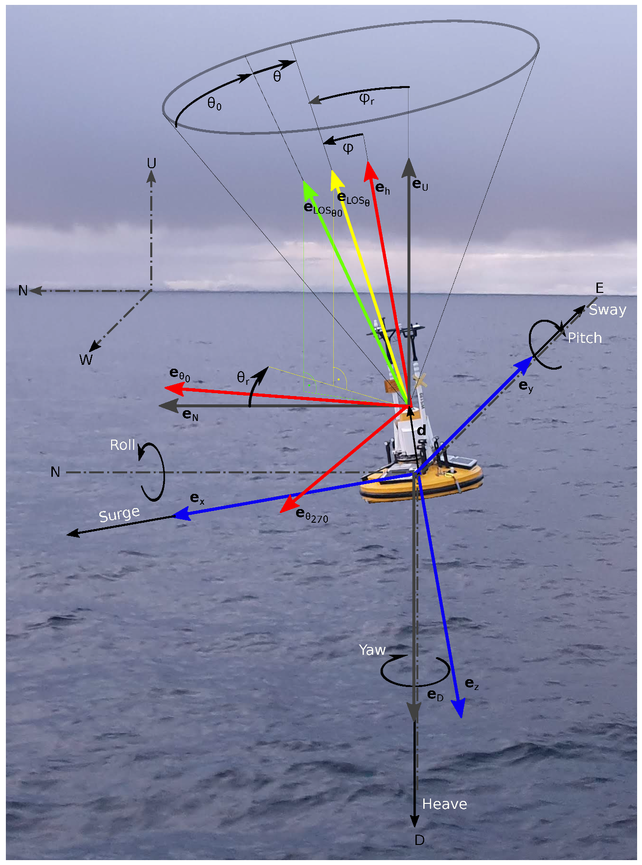
© 2020 by the authors. Licensee MDPI, Basel, Switzerland. This article is an open access article distributed under the terms and conditions of the Creative Commons Attribution (CC BY) license (http://creativecommons.org/licenses/by/4.0/).