Annular Neighboring Points Distribution Analysis: A Novel PLS Stem Point Cloud Preprocessing Algorithm for DBH Estimation

Abstract

Personal laser scanning (PLS) has significant potential for estimating the in-situ diameter of breast height (DBH) with high efficiency and precision, which improves the understanding of forest structure and aids in building carbon cycle models in the big data era. PLS collects more complete stem point cloud data compared with the present laser scanning technology. However, there is still no significant advantage of DBH estimation accuracy. Because the error caused by merging different point cloud fragments has not yet been eliminated, overlapping and inaccurate co-registered point cloud fragments are often inevitable, which are usually the leading error sources of PLS-based DBH estimation. In this study, a novel pre-processing algorithm named annular neighboring points distribution analysis (ANPDA) was developed to improve PLS-based DBH estimation accuracy. To reduce the impact of inaccurately co-registered point cloud fragments, ANPDA identified outliers through iterative removal of outermost points and analyzing the distribution of annular neighboring points. Six plots containing 247 trees under different forest conditions were selected to evaluate the ANPDA. Results showed that in the six plots, error reductions of 53.80–87.13% for bias, 38.82–57.30% for mean absolute error (MAE), and 27.17–56.02% for root mean squared error (RMSE) were achieved after applying ANPDA. These results confirmed that ANPDA was generally effective for improving PLS-based DBH estimation accuracy. It appeared that ANPDA could be conveniently fused with an automatic PLS-based DBH estimation process as a preprocessing algorithm. Furthermore, it has the potential to predict and warn operators of potential large errors during hierarchical semi-automatic DBH estimation.

1. Introduction

Forestry inventory plays an important role in carbon storage estimation, which provides a basis for sustainable management and helps researchers understand terrestrial carbon cycling in the era of big data [1,2]. Of all the forest parameters that can be obtained through nondestructive in-situ measurements, the diameter of the breast height (DBH, 1.30 m height) not only helps researchers understand the structure of a forest but also reflects forest growth state. It contributes to aboveground forest biomass estimation and bridges empirical and process-based models, which directly inform global carbon cycling models [3,4].

For the past few years, an emerging technology known as personal laser scanning (PLS) has shown good potential for in-situ forestry measurements, especially for DBH estimation [4,5,6,7,8,9,10,11,12,13,14]. By the time the concept of PLS was developed, laser scanning technology has been gradually replacing manual DBH measurement due to its high efficiency in collecting accurate data. At present, operational stem-level DBH measurements using laser scanning technology are mainly based on two kinds of methods: static terrestrial laser scanning (TLS) [7,11,13,15,16,17,18,19,20] and vehicle-based mobile laser scanning (MLS) [21,22,23,24,25,26]. Although these methods are reliable for many forest stand conditions, stem-level DBH measurements in a large forest still experience two kinds of problems: occlusion and poor instrument pass ability. Occlusion can cause the TLS point cloud data acquisition in single-scan mode to miss up to 32% trees in sample plots [5]. To ensure data for every stem is collected, the multi-scan mode is always required, which takes a considerable amount of time to mount and dismount the instrument [27]. This is unfeasible when measuring a large area. To improve data collecting efficiency, many vehicles, such as cars [22], vans [23], tractors [26], all-terrain-vehicles [28], and even unmanned aerial vehicles [21,24,25], have been used for vehicle-based MLS. However, the applicability of vehicle-based MLS is usually limited by its instrument pass ability. The beam emitted from ground vehicle-based MLS is often occluded by obstacles and outer trees [22,26], while the beam emitted from UAV-based MLS is often occluded by the canopy [29]. Therefore, stem-level DBH estimation using vehicle-based MLS is not available in many cases. With the concept of personal laser scanning (PLS), there has been a hope for solving these problems. It has high data collecting efficiency and omnidirectional data point distribution. Moreover, it has a good instrument pass ability and allows flexible scanning path selection [7]. PLS has been widely tested for indoor and outdoor mapping [30,31,32,33] and used in cultural heritage sites mapping [34], power line mapping [35], cavity-collapse risks management [36], and automatic 3-D reconstruction of indoor environments [37]. Foresters have recognized that the advantages of PLS mean that it is hardly affected by occlusion and instrument pass ability, which makes it possible to implement the stem-level DBH estimation in more complex forest conditions with high accuracy and efficiency.

From the first experiment conducted by Liang et al. [5] in May 2013 to the present, many studies have demonstrated the feasibility of PLS-based DBH estimation [4,5,6,8,9,10,14]. Comparisons between PLS and other kinds of laser scanning systems have also been made in recent years. Although PLS collects more complete stem point cloud data than TLS, it has lower data accuracy. There was no significant DBH estimation accuracy advantage for PLS in the previous comparisons [7,11,12,13]. This is because when merging point cloud fragments together, inaccurate co-registration is inevitable, and this is one of the leading error sources of PLS-based DBH estimation. While scanning, the inertial measurement unit (IMU) continuously measures the specific force and angular rate. Based on the position and posture data inferred from the specific force and angular rate at every moment, different point cloud fragments are co-registered and merged together. The IMU error thus leads to a cumulative error of position and posture estimation, which is called IMU drift. The IMU drift results in inaccurate co-registration of the point cloud fragments. In the early designs (e.g., AkhkaR2), supporting a global navigation satellite system (GNSS) data was used to reduce IMU drift [9]. However, reliable GNSS data are not always available due to canopy occlusion. In recent years, the most widely applied solution for IMU drift has been simultaneous localization and measurement (SLAM) algorithms. The SLAM algorithms search for common points in different point cloud fragments. Coordinate transform matrixes for co-registration are calculated based on these extracted feature points. SLAM can, therefore, deal with the error caused by IMU drift without dependence on the GNSS signal. However, when the transform matrix is not estimated accurately, incorrectly merged point cloud fragments appear [7]. Although previous researchers have tried various approaches to reduce the error caused by IMU drift, the inaccurate co-registration problem has not yet been properly resolved.

In the inaccurately co-registered fragments, some points are far from the actual stem surface, which leads to errors in implementing DBH estimation. Furthermore, these point cloud fragments usually overlap with the good ones, which makes the error points quite difficult to remove. This kind of error has also been mentioned by Liang et al. [5] and Bauwens et al. [7]. Compared with the previous methods, DBH estimation using PLS data has different problems. The common point cloud preprocessing algorithms are no longer appropriate in theory. However, the present data preprocessing algorithms for DBH estimation using PLS are still mainly based on distantly separated outlier filtering [4,5] or separated cluster removal [8,11]. The efficacy of these methods for the overlapping fragment problem has not been systematically analyzed. To the best of our knowledge, there is currently no algorithm that reduces PLS data-based DBH estimation error due to overlapping, inaccurately co-registered point cloud fragments.

In this study, a novel PLS stem point cloud preprocessing algorithm named annular neighboring points distribution analysis (ANPDA) was developed for the DBH estimation. ANPDA was an algorithm that enhanced circle fitting-based DBH estimation. It reduced the impacts of inaccurately co-registered point cloud fragments by iteratively removing the outermost points from a two-dimensional horizontal projected point cloud. Outliers were identified by analyzing the polar angle distribution of points in the annular neighborhood of the outermost points. The concept of relative entropy was used to quantify the distribution similarity degree and determine the termination criterion for iterative outermost point removal. Points that remained after the critical iteration were grouped and exported as the output point cloud. The methodological contributions of this paper were to (1) support the current PLS-based automatic DBH estimation framework by providing a preprocessing strategy for inaccurate, overlapping point cloud fragments; (2) consider the stem point cloud outlier identification problem based on the polar angle distribution of points in the annular neighborhood; (3) introduce relative entropy to quantify the degree of similarity between point cloud distributions to determine if outliers have been properly removed.

2. Materials and Methods

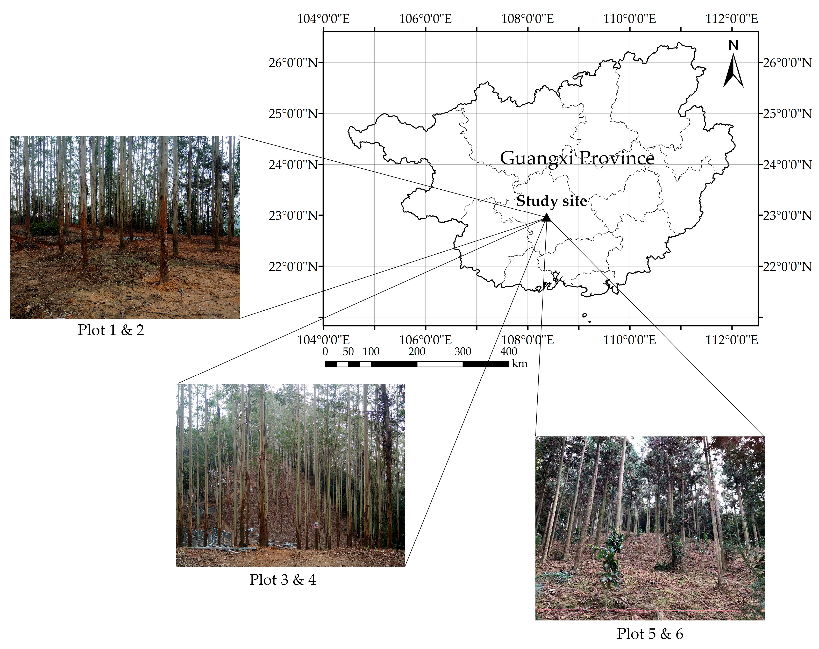
2.1. Study Area

The study site of this study was located in Guangxi Gaofeng state-owned forest farm, which is shown in Figure 1. It is a typical subtropical forest farm in southwest China (22.82°–23.25° N 108.13°–108.88° E). The dominant species of the forest farm are eucalypt and Chinese Fir. Most of the forests grow on the hillside, which makes it difficult for vehicles to enter. Study sites were, therefore, selected in the forest plantation with little understory vegetation to be sure they were accessible for PLS.

To test whether ANPDA could be used for PLS-based DBH estimation under different forest conditions, six plots with a total of 247 trees of different species were selected. Each plot had a fixed size of 25 m × 25 m. Three forest conditions with different degrees of data acquisition difficulty were included to test the adaptability of ANPDA. Plots 1 and 2 had flat and smooth surfaces, which allowed the PLS operator to walk naturally at a steady pace. Plots 3 and 4 were on a machine-graded hillside that made them steep but with a relative tidy slope surface. While collecting data, the PLS operator maintained a low center of gravity for balance at a slower and less steady pace. Plots 5 and 6 were on a hillside with soft and moist soil. While collecting data, extra care had to be taken to avoid slipping. As a result, the sensor might have experienced sudden displacement and spinning.

The forest conditions in the plots are shown in

Table 1. Forest conditions of the test plots.

Plot ID	Species	Number of Trees	Slope	Ground Surface
1	Eucalyptus robusta	52	<5°	smooth and dry
2	Eucalyptus robusta	35	<5°	smooth and dry
3	Eucalyptus robusta	36	>20°	smooth and dry
4	Eucalyptus robusta	39	>20°	smooth and dry
5	Cunninghamia lanceolate and Michelia macclurei	41	>20°	soft and moist
6	Cunninghamia lanceolate and Michelia macclurei	44	>20°	soft and moist

.

2.2. Data Acquisition

To facilitate data acquisition, the experiment was conducted during a less rainy season. All data in this study were collected in January 2018.

2.2.1. Point Cloud Data

The PLS applied in this study was a Heron AC-1 Color wearable mapping system. It was controlled with a tablet and carried on the operator’s back while working. The technical specifications are shown in

Table 2. Technical specifications of the Heron AC-1 Color wearable mapping system.

Weight	6 kg
Time of Initialization	~30 s
Working Time	~3 h/one battery
Indoors/Outdoors Working	Yes
Real-Time Visualization	Yes
Temperature	operating: −10 °C–60 °C storage: −40 °C–60 °C
Output Data	E57, las, ply
Final Global Accuracy	~5 cm in short close rings
Local Accuracy	~2 cm
Final Survey Resolution	~2 cm
Sensor Mounting	Velodyne HDL-32E
Wavelength	903 nm
Max Range	80–100 m
Angular Field of View	Horizontal: 360° Vertical: +10.67°; −30.67°

[38].

For point cloud data acquisition of each plot, the PLS operator walked in an approximate figure-eight shape, which is often used in outdoor point-cloud-based modeling. As shown in Figure 2, the operator began and ended at the center to make a closed route. The practical walking path should be fixed by the operator on the spot with all the stems covered inside the route. After confirmation, the point cloud data was exported and clipped by the operator. While collecting data, rough co-registration was generated in real-time. When the scanning was finished, a more precise co-registration was implemented, which took a few minutes for each plot. The average point density of each plot was 21,028 points/m².

2.2.2. Reference Data

Table 3. Summary of trees in each test plot with a diameter of breast height (DBH) and density.

Plot ID	DBH (cm)			Stem Density (Stems/ha)
	Min	Max	Mean
1	13.4	25.3	21.2	832
2	7.1	27.4	22.5	560
3	10.7	28	20.5	576
4	14.6	25.7	21.0	624
5	12.3	29.9	21.8	656
6	8.9	30.4	20.1	704

summarizes the DBH and density of trees in each plot. The DBH of the stems varied from 7.1 cm to 30.4 cm, with a density of 560 to 832 stems/ha. Each stem was indexed, and the DBH was manually measured using diameter tape. The position of each stem in each plot was then measured with the total station according to the index. These positioning data were collected to match the manually measured DBH with the stem point clouds, so positioning errors at the decimeter level were acceptable. The impact of the stem diameter for positioning was, therefore, ignored. Reference positioning maps of stems were then generated with DBH according to the index.

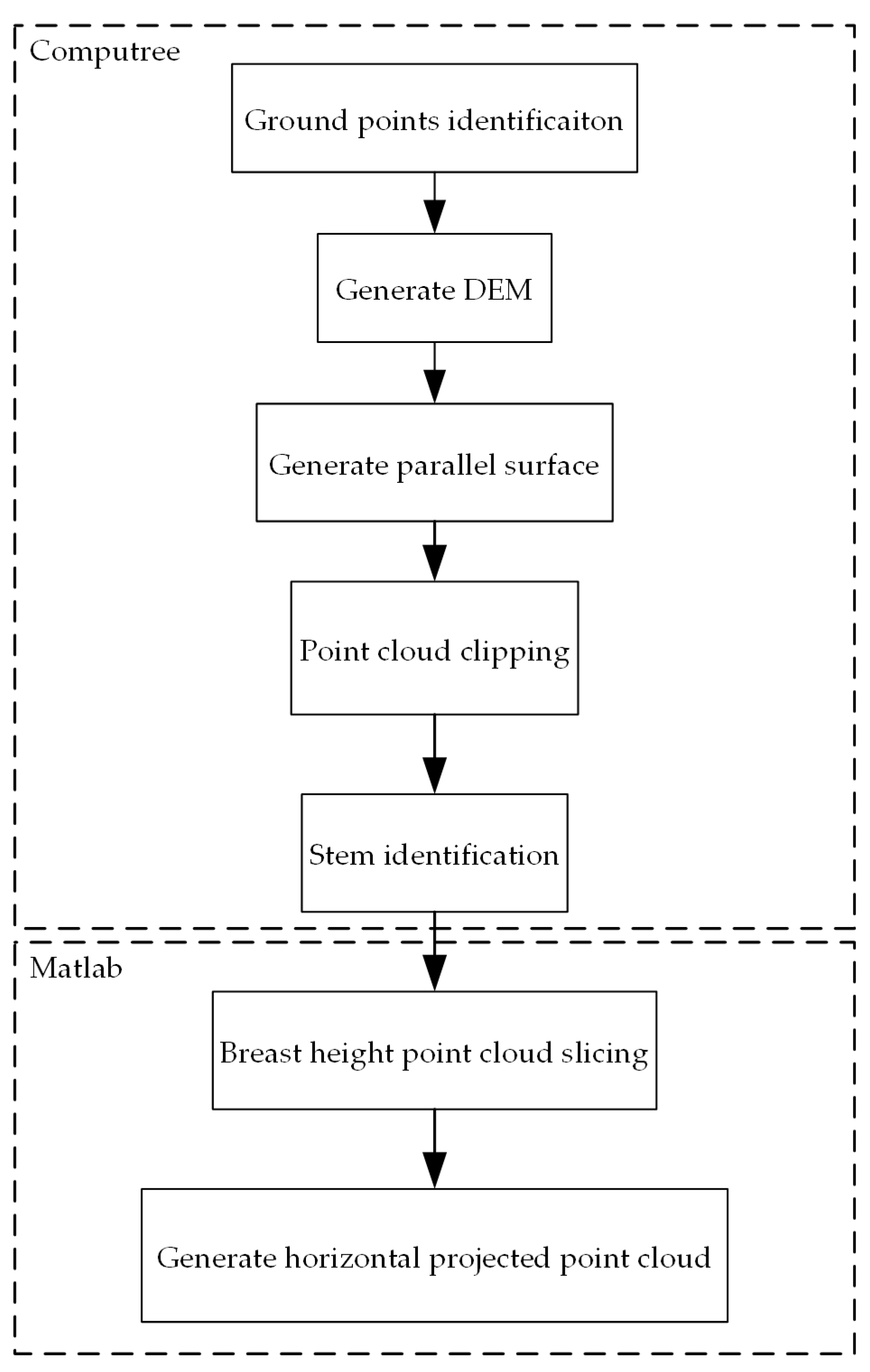
2.3. Essential Data Processing before Implementing ANPDA

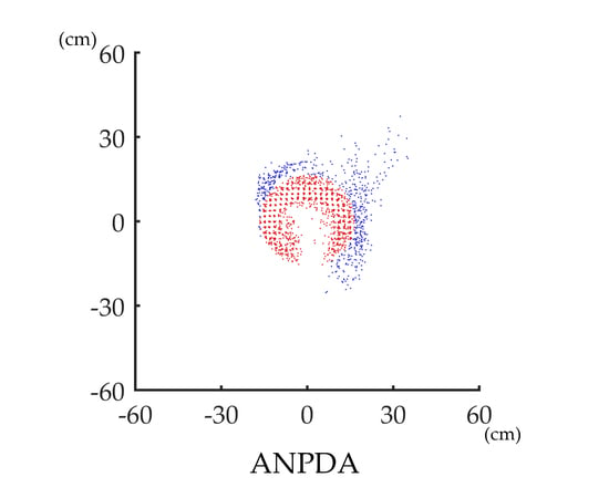
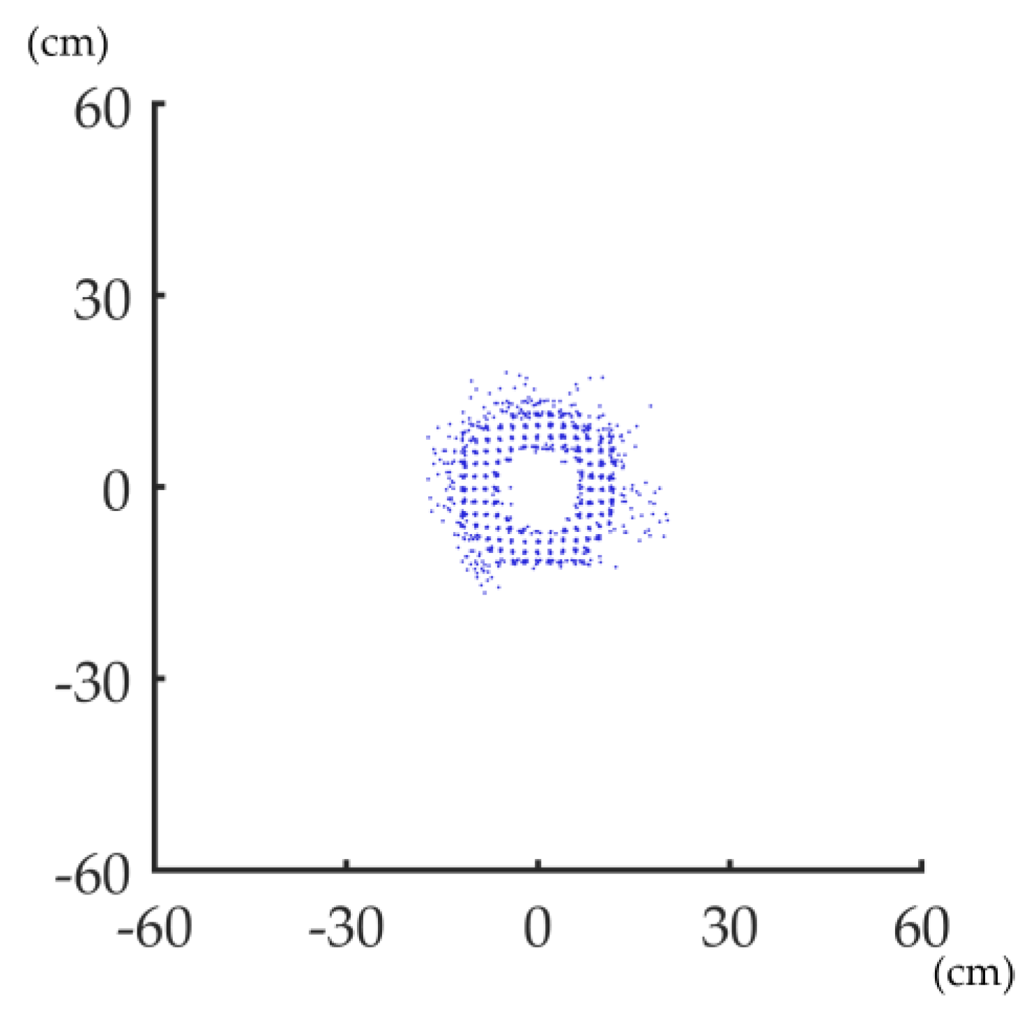
ANPDA is a pre-processing algorithm, dealing with the two-dimensional horizontal projected point clouds of stems at breast height. It is essential to generate projected point clouds before applying ANPDA. For each plot, the points of ground were first identified. A digital elevation model (DEM) of the plot was generated and rasterized. Based on the rasterized DEM, a 2 m-height surface of the plot parallel to the DEM surface was generated. The point cloud was clipped to retain the points between the two surfaces. Clustering analysis was then implemented. The clusters were regarded as stems, and the horizontal cluster center was approximately the horizontal stem center. The identified stem point clouds were then clipped into vertical slices. Considering the possible bias of the horizontal stem center and the tree density of the plots, the side length of the vertical clipping square was set at 2 m. Based on prior research [19], the vertical point cloud slice thickness was set to be 20 cm to guarantee circle fitting accuracy. The point cloud for each stem was clipped with only 2 m × 2 m × 0.2 m cubic space remaining. The center of the cubic space was 1.3 m above the DEM surface, with the same horizontal coordinate as the coordinate of the horizontal cluster center for each stem. The point cloud data were then projected onto the horizontal plane for circle fitting. Finally, the projected point cloud data for identified stems were indexed and recorded.

To simulate automatic DBH estimation processing, two software packages were used in this study. As shown in Figure 3, the procedures from ground point identification to stem identification were conducted with Computree [39]. Computree performs batch processing for forest point cloud data in a pre-determined order determined by the user. The algorithms of the applied plugins have been described in [40]. As a supplement, point cloud slicing and projection were implemented with MATLAB [41]. The positioning maps of identified stems were compared with the reference positioning maps to match projected point clouds with the reference data manually.

2.4. ANPDA

In this section, an overview of ANPDA is given first, which describes the rationale behind ANPDA. A flow chart of how ANPDA works is also shown and explained in the first subsection. The technical details of each step are described in the following subsections.

2.4.1. Overview

To understand how ANPDA works, a basic understanding of the error is essential. Under ideal conditions, the stem surface is approximately a cylinder, which means the projection should be approximately a circle. Figure 4 shows a PLS-based horizontal projected stem point cloud with good co-registration. The projected point cloud is scattered in the shape of the ring. It is sparse in the inner and outer layers and dense in the middle.

Figure 5a,b shows a PLS-based horizontal projected stem point cloud with inaccurately co-registered fragments. In the point cloud with incorrect co-registration, some fragments bulge out of the surface. The projected point cloud looks like a ring with some crescent fragments inserted on it. The point cloud fragments with inaccurate and good co-registration are overlapping. There is no exact boundary between them. Thus, it is difficult to filter out the overlapping inaccurate co-registered fragments. In those inaccurately co-registered fragments, some points are far from the real stem surface, which usually leads to significant DBH overestimation for algorithms based on circle fitting. The developed ANDPA method identified the bulgy points as outliers before removing them for a better DBH estimation. These outliers usually distribute far from the fitting circle center. If there are any outliers outside the fitting circle, they are most probably the farthest from it. To describe such points, the concept of the outermost point is involved. Here, we defined the outermost point of the projected point cloud as the point farthest from the fitting circle center. Figure 5c shows an example of the identification of the outermost point.

ANPDA iteratively analyzes and removes outermost points to filter outliers, which was inspired by lathing. An iterative analysis is first implemented. In each iteration, the outermost point is analyzed and removed from the projected point cloud. After that, the projected point cloud and the fitting circle center is updated. According to the results of the iterative analysis, the ideal number of iterations for removing outliers is determined. The points remaining after this iteration are exported as the output.

To determine when the iterative point removal process should end, the annular neighborhood of the outermost point was also involved in this study. We defined the distance between the outermost point and the fitting circle center as R. The distance between the inner and outer circle was described as pre-determined thickness value t. The annular neighborhood of the outermost point was an annular area with the center located on the fitting circle center. The outer radius was R, and the inner radius was max((R − t), 0). Figure 6 shows an example of the annular neighborhood of the outermost point.

Figure 7 shows an example of the polar angle distribution of the points within the annular neighborhood and all the remaining points while iteratively removing the outermost points. All points are divided into groups with equal polar angle range. The probability distribution of the polar angle is used to describe the polar angle distribution. In Figure 7a–c, the outermost point is an outlier. The polar angle distribution of the points within the annular neighborhood tends to be centralized around a certain angle. The distribution is very different from that of the remaining points. In Figure 7d, the outermost point tends to have good co-registration. All the points located farther from the center than this well co-registered point have already been removed. It means most of the outliers have been filtered out. The polar angle distribution of the points within the annular neighborhood is thus relatively uniform and similar to that of all remaining points. The degree of similarity is quite close for all the outermost points with good co-registration compared with the outliers. This becomes a distinguishing criterion that is adopted by the algorithm.

The strategy for determining whether the outliers have been adequately removed is based on the characteristics of the two kinds of polar angle distributions mentioned above. In the iterative analysis, with the outermost points iteratively removed, the degree of similarity in each iteration is quantified to show the variability. If there is a trend that the polar angle distributions of points in the annular neighborhood and the remaining points were becoming more similar, it means the number of outliers is still decreasing significantly with the removal of the outermost points. When the degree of similarity is relatively stable, it means the outliers have already been properly removed. Once the critical point between these two states is found, the termination criterion for outermost point removal iterations is determined.

ANPDA was designed based on the ideas described above. The overall flow of the algorithm is illustrated in Figure 8.

As illustrated in Figure 8, the imported projected point cloud was first set as the current point cloud. The algorithm iteratively analyzed and removed points. In each iteration, circle fitting was implemented first. The center of the fitting circle was called point O. The outermost point of the point cloud was identified and called point M. The polar angle probability distributions for points in the current point cloud and in the annular neighborhood of M were calculated. For both point clouds, O was set as the origin. The polar angle of each point was made with the positive direction of the x-axis. The degree of similarity between the two distributions was quantified as value S based on relative entropy. The index of the outermost point, the index of the current iteration, and value S were recorded for future analysis. At the end of each iteration, the outermost point M was removed, and the current point cloud was updated. After the iterative analysis, the suitable iteration number N for point removal was calculated based on the recorded similarity value S. From the initially projected point cloud, all outermost points recorded in the first N iterations were removed. The remaining points were exported as the output point cloud.

The technical details of each step are further described in the following subsections.

2.4.2. Circle Fitting

The circle fitting algorithm used in ANPDA is the Landau algorithm [42], which was implemented by Sumith [43] and proved to be reliable for DBH estimation based on TLS point cloud data by Chang et al. [19]. The Landau algorithm is a non-iterative linear least square algorithm. The error is defined as the difference between the area of the fitting circle and the area of the circle with the same center and a radius of R^’, where R^’ is the distance from the point to the center. By minimizing the squares of error, the radius and coordinates of the fitting circle center are acquired.

Because ANPDA is an iterative algorithm, a non-iterative circle fitting algorithm like the Landau algorithm can effectively reduce computation time.

2.4.3. The Choice of the Annular Neighborhood Thickness Value

To implement the annular neighboring points analysis, an appropriate thickness value for the annular neighborhood is required. When the thickness value of the annular neighborhood is too low, the polar angle distribution of the points in the annular neighborhood can be easily influenced by random error. The fluctuation of the similarity degree would influence the judgment of outliers. When the thickness value is too high, the algorithm is insensitive to the outliers near the good points because they have a similar annular neighborhood. Considering the PLS-based stem point cloud resolution, a thickness value of 0.5 cm was used in this study.

2.4.4. Polar Angle Probability Distribution Analysis

In this study, the polar angle for each point was defined in the polar coordinate system, with the fitting circle center as the origin. The polar angle of each point was made with the positive direction of the x-axis. Figure 7 also shows an example of calculating the polar angle probability distribution of a point cloud. For convenient calculation, the polar angle was converted into a value ranging from [0, 2π). The probability distribution of the polar angle was used to describe the polar angle distribution of the points in a point cloud. All points were divided into equal groups based on the polar angle range. The interval of each group was [0, 2π/N_g), [2π/N_g, 4π/N_g), …, [2π(N_g − 1)/N_g, 2π), where N_g denotes the number of groups. The probability distribution of the polar angle was recorded in a set as {P₁, P₂, …, $P_{N_g}$}, where P_i denotes the probability of the polar angle of any point in the interval of [2π(i − 1)/N_g, 2πi/N_g), which can be calculated by Equation (1):

$$P_i=\frac{n_i}{n_{\mathrm{all}}}$$

(1)

where n_i denotes the number of the points with a polar angle ranging from [2π(i − 1)/N_g, 2πi/N_g), and n_all denotes the number of the points in the current point cloud. In this research, the number of groups was set to be eight.

2.4.5. Distribution Similarity Quantification

To quantify the degree of similarity between the polar angle distribution of the points in the annular neighborhood of the outermost point and all the points in the current point cloud, the concept of relative entropy is used. Relative entropy, also known as Kullback–Leibler Divergence, was first developed by Kullback et al. [44]. Now it is widely used for evaluating information that is lost when a real distribution is substituted by an approximate distribution. From another perspective, it also reflects whether a distribution is approximating another one. In Equation (2), $KL(P\parallel Q)$ denotes the relative entropy, P(x), Q(x) are the two probability distributions, and Q(x) is the distribution used to substitute P(x). The relative entropy value is non-negative. When both distributions are the same, the relative entropy value is 0. A higher relative entropy value represents a greater difference between the two distributions. As relative entropy is not symmetric, it cannot be used to measure the distance between the two distributions.

$$KL(P\parallel Q)={\displaystyle \sum _{i=1}^{n}P(x)\log \frac{P(x)}{Q(x)}}$$

(2)

Based on the knowledge of relative entropy, the similarity value of the current point cloud is defined in Equation (3) to quantify the degree of similarity between the polar angle distribution of points in the annular neighborhood of the outermost point and all the points in the current point cloud.

$$S={\displaystyle \sum _{i=1}^{N_{\mathrm{g}}}{P}_{\mathrm{ann}}(x)\ln \frac{P_{\mathrm{ann}}(x)}{P_{\mathrm{cur}}(x)}}$$

(3)

In Equation (3), S denotes the similarity value, while N_g denotes the number of groups. P_ann(x), P_cur(x) denote the polar angle probability distribution of the points in the annular neighborhood of the outermost point and all the points in the current point cloud, respectively. For computational convenience, a natural logarithm is applied. It can be seen from Equation (3) that a smaller similarity value indicates that the polar angle distribution of the points in the annular neighborhood point cloud and the polar angle distribution of the points in the current point cloud are more alike, and vice versa.

2.4.6. The Termination Criterion

ANPDA mainly consists of two parts: distribution analysis and outlier removal. Both the two parts are implemented iteratively. Therefore, the termination criteria are essential.

The aim of iterative distribution analysis is to show the variability of similarity value and find the critical point when the outliers are properly removed. Considering ANPDA’s outlier identification strategy, more iterations theoretically provide more data to describe when the similarity value becomes relatively stable after the outliers have been properly removed. Under ideal conditions, the iteration should continue until there are so few points remaining that the polar angle distribution would be easily influenced by random error. However, there is still a type of error that requires practical attention. A projected point cloud is usually in the shape of a ring. Although the outliers outside the outer circle of the ring cause the main error, there are still many points with big error inside the inner circle. During the analysis, the outermost points are iteratively removed. After removing most points with good co-registration, the proportion of the inside error points can be quite high. When the current point cloud consists of insufficient remaining points, it is also not well co-registered. These point clouds are not suitable for describing the characteristics of a good co-registered point cloud and should be excluded from the iterative distribution analysis. Considering the above, the termination criterion of iterative distribution analysis is determined. In this study, a minimum remaining points number of 500 was used to reduce the influence of the inner error points.

To operationalize the outlier identification strategy described above, the termination criterion for iterative outlier removal is determined based on the variability of the similarity value. The critical iteration should be the one when the similarity value becomes approximately stable. For operational convenience, the critical point is determined to be the iteration in which the decline of the similarity value first approaches the average of the similarity value of all remaining iterations. All points removed prior to that iteration are regarded as outliers. The termination criterion of outlier removal can be written as Equation (4):

$$S_i\le \frac{1}{I-i}{\displaystyle \sum _{j=i+1}^I{S}_j}$$

(4)

where S_i denotes the similarity value of iteration I, and I denotes the number of iterations in the iterative distribution analysis. Figure 9 shows an example of the final iteration for outlier removal and the remaining point cloud.

2.5. Evaluation of ANPDA

Improvements in DBH estimation accuracy after applying ANPDA were used to evaluate ANPDA performance. The DBH estimated from projected point cloud data before and after applying ANPDA were compared to determine whether ANPDA was effective. Bias, mean absolute error (MAE), and root mean squared error (RMSE) facilitated the evaluation with the following equations:

$$Bias=\frac{1}{n}{\displaystyle \sum _{i=1}^n(d_i-D_i)}$$

(5)

$$MAE=\frac{1}{n}{\displaystyle \sum _{i=1}^n\left|d_i-D_i\right|}$$

(6)

$$RMSE=\sqrt{\frac{1}{n}{\displaystyle \sum _{i=1}^n{(d_i-D_i)}^2}}$$

(7)

where n denotes the number of stems, d denotes the estimate, and D denotes the reference. The Landau circle fitting algorithm described in Section 2.4.2 was applied for DBH estimation.

Inevitably, some stem point cloud slices were unqualified due to poor automatic stem identification and point cloud segmentation algorithms. A forked stem (crevice or crotch shape stems formed by doubletree trunks) might be identified as a single stem. Some clipped stem point cloud slices were mixed with points of leaves and wrapping branches. Because the main concern of this research was whether ANPDA was effective in reducing the influence of incorrect point cloud fragments registration, stems with point cloud segmentation problems were counted but not used for evaluating ANPDA. The results were then compared with the reference data.

In prior research, the performance of PLS-based DBH estimation was evaluated with the estimation accuracy [5,6,8,9]. However, the quality of stem point cloud data is various and has a massive impact on estimation accuracy. Evaluating a DBH estimation method just by the final estimation accuracy is not sufficient. This study also considered how effective ANPDA was for the data of different quality. We used the mean squared error (MSE) to evaluate the quality of the horizontal point cloud slices according to how well the horizontal projection fits a circle. MSE is a well-known indicator that has been used to evaluate DBH estimation by former researchers [45]. In this study, it provided a measure of how a projected point cloud could be replicated by the fitting circle using least squares. Based on the error defined by the Landau algorithm, the MSE was derived using Equation (8):

$$MSE=\frac{1}{n_{\mathrm{p}}}{\displaystyle \sum _{i=1}^{n_{\mathrm{p}}}{\left\{\pi R^2-\pi \left[{\left(x_i-\overline{x}\right)}^2+{\left(y_i-\overline{y}\right)}^2\right]\right\}}^2}$$

(8)

where MSE denotes the mean squared error, n_p denotes the number of the points in the point cloud, (x_i, y_i) is the coordinate of a point, and $(\overline{x},\overline{y})$ is the coordinate of the center of the fitting circle. To facilitate horizontal point cloud classification, value p, which was the natural logarithm of MSE, had been used. It made the number of samples in each group more even. Value p was calculated using Equation (9):

$$p=\ln MSE=\ln \left(\frac{1}{n_{\mathrm{p}}}{\displaystyle \sum _{i=1}^{n_{\mathrm{p}}}{\left\{\pi R^2-\pi \left[{\left(x_i-\overline{x}\right)}^2+{\left(y_i-\overline{y}\right)}^2\right]\right\}}^2}\right)$$

(9)

All the horizontal point cloud slices were classified according to the value p. A smaller p means the distribution of the projected point cloud is more similar to a circle, which usually means better data quality. To assess whether ANPDA was reliable for stem-level inventory in each class, the effective rate was also calculated with Equation (10):

$$Effectiverate=\frac{n_e}{n}\times 100\%$$

(10)

where n denotes the number of the stems, and n_e denotes the number of stems that achieved a smaller estimation error after applying ANPDA. The average error reduction after applying was also calculated to evaluate the efficacy, with Equation (11):

$$Averageerrorreduction=\frac{1}{n}{\displaystyle \sum _{i=1}^n\left|\left|d_i-D_i\right|-\left|{d^{\prime }}_i-D_i\right|\right|}$$

(11)

where n denotes the number of stems, d denotes the estimate after applying ANDPA, $d^{\prime }$ denotes the estimate without applying ANDPA, and D denotes the reference. The relationship between data quality and the effectiveness of ANPDA has been described based on these results.

3. Results

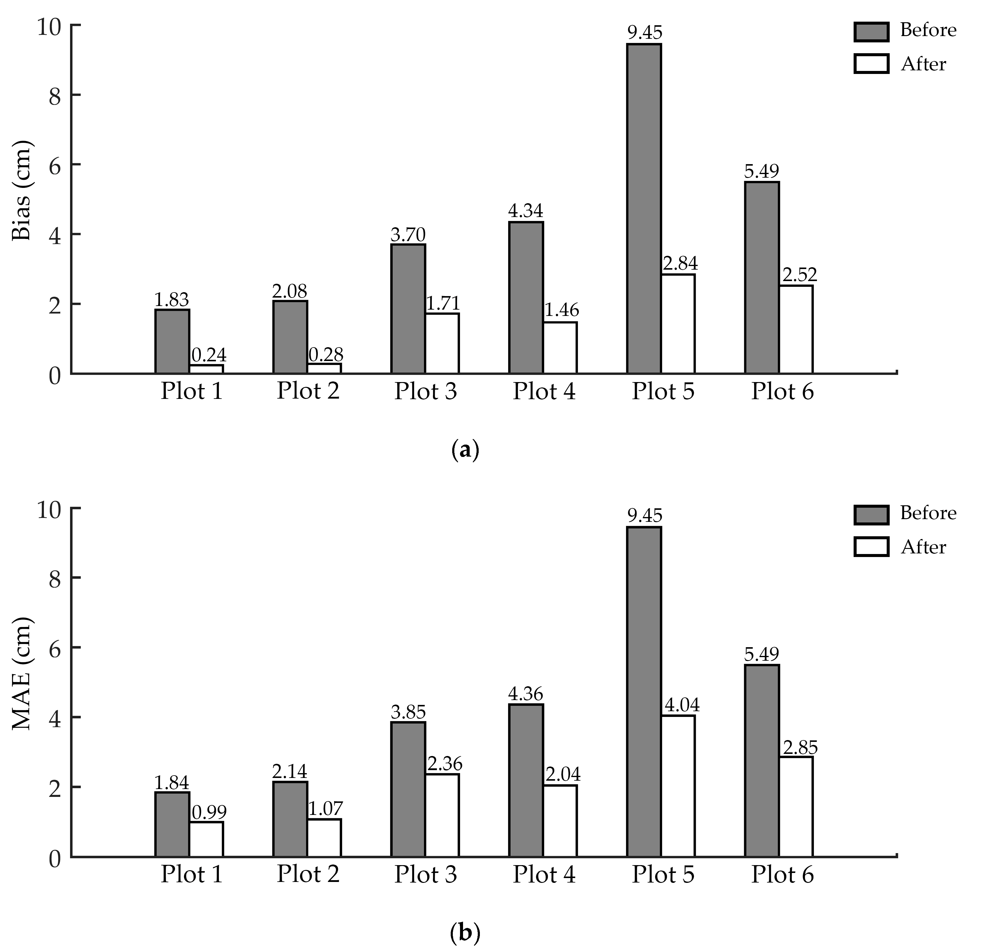
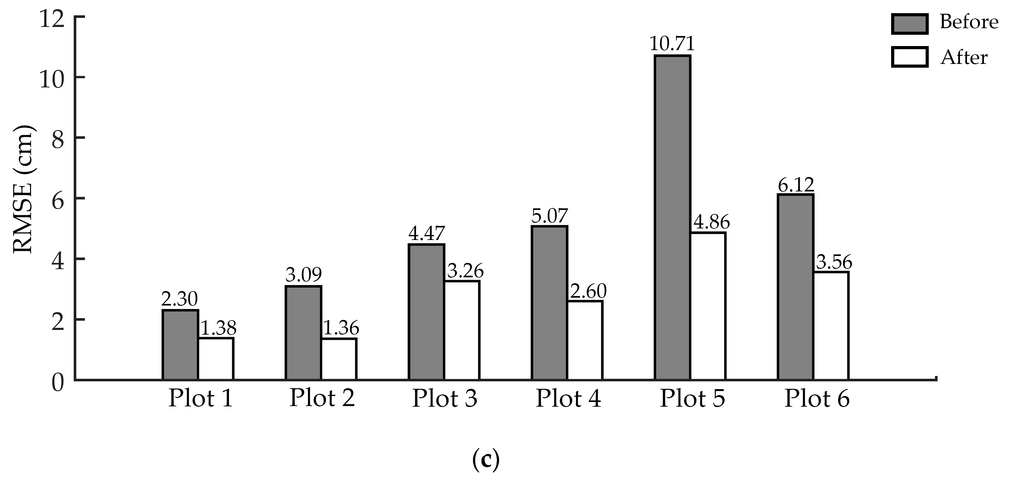
3.1. The Performance of ANPDA in Different Test Plots

The performance of ANPDA was tested in all six test sites. The scanning time for each plot was less than ten minutes. The processing time of applying ANPDA was about one minute for each plot with an Intel(R) Core(TM) i7-4700MQ CPU @ 2.40 GHz processor. Of the 247 stem horizontal point cloud slices clipped from the identified stems, five had the forked stem problem, while 13 of the horizontal point cloud slices were wrapped by branches and leaves. With the exception of these unqualified stem point cloud slices, the remaining 229 slices did not have huge errors arising from automatic stem identification and segmentation algorithms. All 229 qualified horizontal stem point cloud slices were used for evaluating ANPDA.

Figure 10 shows the DBH estimation accuracy before and after applying ANPDA. It could be seen from the results that in all the six test sites, there was a decline in all three accuracy indicators (bias, MAE, and RMSE) that were used to reflect the error. As shown in Figure 10, before ANPDA was applied, the bias of the estimated DBH for the six test sites was distributed around 1.83–9.45 cm, which showed a general trend of overestimation. The MAE and RMSE was 1.84–9.45 cm and 2.30–10.71 cm, respectively. Among the three kinds of working conditions, the estimation accuracy was best in the flat plots with the dry and smooth ground surface and worst for the slopes with the moist and soft ground surface. After implementing ANPDA, the reductions were 1.59–6.61 cm for bias, 0.85–5.41 cm for MAE, and 0.92–5.85 cm for RMSE.

Table 4. Error reduction rates for bias, mean absolute error (MAE), and root mean squared error (RMSE) under different forest conditions after applying annular neighboring points distribution analysis (ANPDA).

Plot ID	Number of Qualified Stem Point Clouds	Error Reduction Rates after Applying ANPDA
		Bias	MAE	RMSE
1	52	87.13%	46.20%	39.96%
2	34	86.36%	49.84%	56.02%
3	32	53.80%	38.82%	27.17%
4	39	66.27%	53.06%	48.76%
5	30	69.92%	57.30%	54.61%
6	42	54.09%	47.99%	41.92%

shows the improvement of DBH estimation accuracy in all six test sites. The bias of the estimation was from 0.24–2.84 cm. The reduction rate of the bias was 53.80–87.13% after applying ANPDA, which showed high reliability at the plot level. The reduction rates of MAE and RMSE were 38.82–57.30% and 27.17–56.02%, respectively. It meant that the variation of the DBH estimation around the reference data had decreased. The estimation became more reliable after applying ANPDA. It could be seen from Figure 10 and Table 4 that after applying ANPDA, the bias, MAE, and RMSE of the DBH estimation results decreased in all six test plots. These results showed good adaptability of ANPDA for different working conditions.

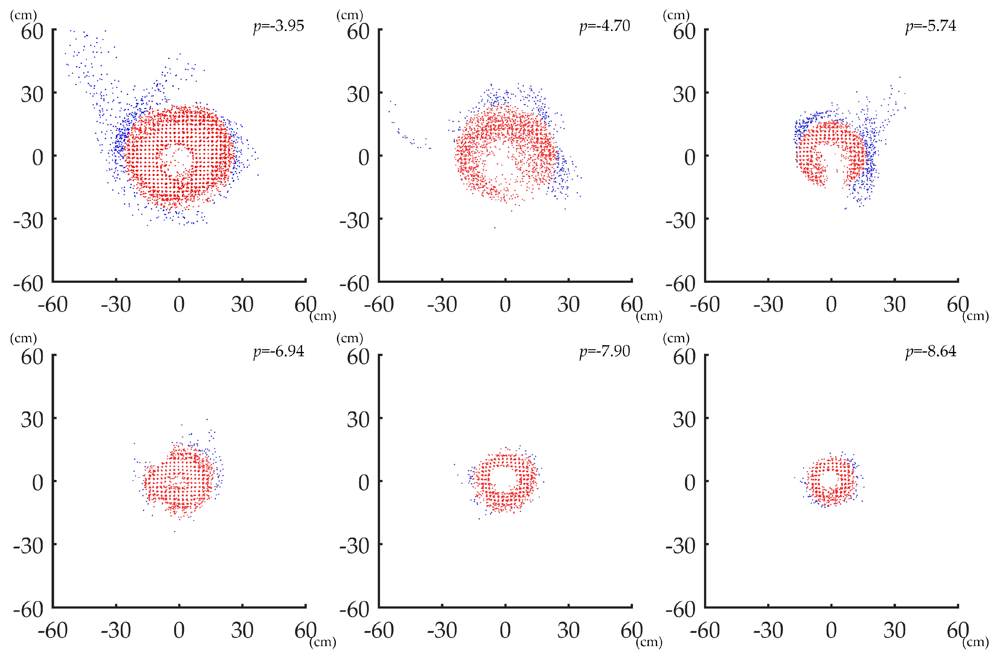
3.2. The Performance of ANPDA for Horizontal Stem Point Cloud Slices of Different Quality

After classifying the qualified horizontal point clouds with value p, the performance of ANPDA for point cloud slices of different quality was analyzed. Figure 11 shows that without applying ANPDA, the data of lower quality led to higher DBH estimation error. After applying ANPDA, the difference in the error for all six classes became smaller. There was a decline in all three accuracy indicators for the DBH estimation error after applying ANPDA.

Table 5. The effective rates of ANPDA.

p-Value	Number of Qualified Stem Point Clouds	The Average of Error Reduction (cm)	Effective Rate
−9 to −8	6	1.16	66.67%
−8 to −7	126	1.19	81.75%
−7 to −6	64	1.73	89.06%
−6 to −5	20	3.67	100.00%
−5 to −4	10	3.67	100.00%
−4 to −3	3	2.78	100.00%

shows the average error reduction and the effective rate of applying ANPDA. Aside from the class with a p-value of −4 to −3, which only contained three-point clouds, the average error reduction and effective rate of ANPDA decreased as the value of p decreased. This indicated ANPDA performed better for data of lower quality. Aside from the class with a p-value of −9 to −8, which only had six samples, the effective rate of ANPDA was generally higher than 80%. This reflected the reliability of ANPDA for horizontal point cloud slices of different quality at the single tree scale.

Table 6. Error reduction for point cloud slices of different quality after applying ANPDA.

p-Value	Number of Qualified Stem Point Clouds	Error Reduction of DBH Estimation
		Bias	MAE	RMSE
−9 to −8	6	63.05%	38.39%	39.79%
−8 to −7	126	66.82%	40.00%	32.23%
−7 to −6	64	62.79%	47.98%	42.30%
−6 to −5	20	67.72%	56.17%	47.25%
−5 to −4	10	71.65%	69.39%	62.87%
−4 to −3	3	68.95%	68.95%	68.88%

shows the improvement in DBH estimation accuracy for all six classes based on p. The error reductions of 62.79–71.65% for bias, 38.39–69.39% for MAE, and 32.23–68.88% for RMSE were achieved. These results indicated that ANPDA was generally effective for stem point clouds of different quality.

Figure 12 shows examples of applying ANPDA on point clouds of different data quality. The blue points represent the points that were removed, while the red points make up the output point clouds. The points of the point clouds with higher p-value usually have a more discrete distribution. After applying ANPDA, the bulged points in point clouds of different quality were excluded, and the surface of the point clouds became smoother and more similar to a circle.

4. Discussion

4.1. The Adaptivity of PLS for Forest Stands on the Slope

To test whether ANPDA was widely applicable for practical work, experiments were carried out in the forest plantation on the hillside with typical working conditions in southwest China. The six test plots represented three different working conditions: (1) flat plots with dry and smooth ground surface; (2) plots on a slope with the dry and smooth ground surface, and (3) plots on a slope with the moist and soft ground surface. In prior studies, the DBH estimation error for PLS-based data was usually from 1–4 cm for RMSE [4,6,7,8,9,10,11,12,13,14]. However, this accuracy level was not always achieved in this study. Without applying ANPDA, only the data acquired in condition (1) had a relatively good estimation accuracy. The estimation accuracy was best in the walkable flat plots and worst for the slopes with the moist and soft ground surface, which also proved the impact of working conditions for DBH estimation. This is because whether the scanner can work steadily severely impacts the data accuracy. When PLS was working on a slope, especially a slope with the moist and soft ground surface, the PLS operator needed more actions to avoid danger. These actions caused sudden moves and rotations of the sensor, which led to more IMU drift. The DBH estimation accuracy was, therefore, reduced.

In this study, all the test plots were located in the forest stands on the hillside. Walking across the forest was the only non-destructive way to reach the test plot, meaning vehicle-based MLS was not available. The efficiency was also a factor that had been counted. In prior research, Giannetti et al. [12] attempted to compare TLS with PLS. Although multi-scan TLS had higher DBH estimation accuracy (with the RMSE 0.15 cm lower than PLS) using scans of 1-h in total, PLS data obtained almost the same accuracy with only seven minutes of walking. Oveland et al. [13] compared three different ground-based laser scanning methods: TLS, hand-held PLS, and backpack PLS. The backpack PLS had the shortest working time of 16 min, the highest tree detection rate of 87.5%, and the highest DBH estimation accuracy with an RMSE of 2.2 cm. Considering the time and labor caused by repetitively mounting and dismounting instruments on the slope, TLS was also not a good choice in this research. Among all the laser scanning techniques, PLS might be the only one that is adaptive for forest stands in the mountainous area due to its portability and good pass ability. It could have become the most appropriate solution if the DBH estimation accuracy was ensured. However, in this study, the accuracy of direct DBH estimation was not satisfying because of the poor working conditions in which the scanner could not work steadily. According to the results, direct DBH estimation using PLS data did not always lead to reliable DBH estimation accuracy on the slopes. After applying ANPDA, the estimation accuracy was improved and achieved the accuracy level in prior research. The adaptivity of ANDPA for poor working conditions showed good potential for making up the gap of DBH in-situ measurement solutions.

4.2. ANPDA for Horizontal Point Cloud Slices of Low Quality

According to the results, ANPDA performed better for data of lower quality. The average error reduction and the effective rate of ANPDA decreased as p decreased. This could be because ANPDA deals with outliers outside the fitting circle and works better when the error source is mainly from outside. For projected point clouds of low quality, the points outside the circle were usually far away from the fitting circle and were a more important error source. When the data quality was sufficiently good, the error from outside was not much higher than the error from other sources, which might have made the efficacy of ANPDA less significant.

DBH estimation usually achieves a lower accuracy using data of lower quality, which can also be inferred from the results. In prior research, some data sets were even excluded from the research because of their low data quality [7]. With the application of ANPDA, relatively reliable results were derived from low-quality data, which confirmed that ANPDA had the potential to reduce the essential manual intervention while estimating DBH. Its adaptivity to low-quality data also made automatic DBH estimation less sensitive to specific abnormal data. While modeling, retaining a more complete data set would make the sample plots more representative as well.

4.3. ANPDA for Other Error Sources

Practically, errors are not always caused by co-registration. Sometimes, the error in PLS-based DBH estimation is caused by points that do not belong to the trunks [11]. In this study, ANPDA showed good adaptability for some of these errors. It was also effective for dealing with the occluding objects that were clustered in a specific direction, such as vines, falling bark pieces, independent branches. Nevertheless, for stems surrounded by branches and leaves, the DBH estimation accuracy was still not high enough after applying ANPDA. It should be also noted that ANPDA did not apply to the forked stem problem. This was because ANPDA tends to regard an outermost point as an outlier when the polar angle distribution of the points in its annular neighborhood is different from all the points in the point cloud. Therefore, it helped remove points from occluding objects when the polar angle was distributed around a specific value. However, when the amount of the error points was too big, or they were uniformly distributed around, ANPDA was no more applicable. For forked stems, the center of the stem would be regarded as a point between the two trunks while implementing circle fitting, which led to incorrect estimation. Stem point cloud segmentation algorithm for covering branches and forked stems is suggested in future studies while implementing ANPDA.

4.4. ANPDA for Automatic and Hierarchical Semi-Automatic DBH Estimation

To explore the full potential of PLS, automatic data processing was a primary concern in this study. In prior research, a mostly applied processing framework was “ground point identification-stem positioning-breast height point cloud slicing-DBH extraction” [4,5,10,12,13,14]. Although not all the researchers have declared clearly whether their processing was automatic or not, their attempts have already confirmed this framework to have great potential for automatic DBH estimation. For automatic processing, the algorithmic complexity is crucial. ANPDA has introduced a non-iterative circle fitting algorithm, the Landau algorithm. It has avoided applying an iterative algorithm in another one. The algorithmic complexity is, therefore, reduced from O(n²) to O(n). That’s the reason why the computational time for each plot is only about one minute. The experiments in this study showed that ANPDA could be fused appropriately with the current automatic processing framework as a preprocessing module between breast height point cloud slicing and DBH extraction. However, it also reflected the limitations of the current framework. There were still a number of point clouds for which acceptable DBH estimation results were not available, regardless of whether ANPDA was applied, which meant that ANPDA might not be suitable for these types of errors. In the current automatic DBH estimation framework, when the data processing method was not suitable for some of the point clouds, which could not be foreseen ahead of time, the errors were typically so large that even the error from a few stems could be as large as the sum of the errors from all the other stems in the plot. To ensure that the results estimated from these “unqualified” point clouds would not ruin the whole experiment, researchers might need to check all the point clouds by visual interpretation [7]. On the one hand, this is contrary to the original intention of automation, and on the other, when collecting point cloud data for a forest at a scale larger than plot level, the time and labor costs of visual interpretation may not be acceptable.

According to the reasons above, we suggested that the problem could be solved using hierarchical semi-automatic processing, which has also been attempted by Cabo et al. [11]. A semi-automatic filtering module can be added after breast height point cloud slicing. By analyzing the features of the data sets themselves, the algorithm attempts to identify the data sets that could lead to unacceptable large error. Only these data sets would be sent to the human operators for visual interpretation and manual intervention, which may lead to significant labor savings due to improved accuracy. For ANPDA, this feature can be the p-value. As shown in Figure 11, higher p values typically produce larger errors. It is recommended that the relationship between the data quality of horizontal point cloud slices and the final error be explored in future research so that ANPDA can be applied in a more robust and flexible way through hierarchical semi-automatic processing.

In the present DBH estimation framework, ANPDA was more like a remedial measure for making up the accuracy loss caused by inaccurate co-registration of point cloud fragments. Future research should also pay more attention to point cloud fragment co-registration algorithms. Avoiding inaccurate registration and removing low-quality point cloud fragments might be the key to obtaining higher accuracy results.

4.5. Outlook

To achieve the optimal performance of ANPDA, more experiments should be taken in future research. Influenced by the laser scanners and co-registration algorithms, the form of PLS point cloud can be various. Unlike the overestimation shown in the results of this study, some instruments, such as the ZEB1 handheld mobile laser scanner, can also cause underestimation [6,12,14]. More PLS instruments should be used to acquire a better understanding of the error and improve ANPDA. The determination strategy of the parameters should be studied in future research to achieve the optimal performance of ANPDA. Iterative points removal from inside to outside can also be attempted as a supplementary.

In prior research, circle fitting-based DBH estimation has been developed into a mature method [7,8,9,11]. However, a number of PLS-based DBH estimation experiments have been conducted using a cylinder fitting approach [4,5,6,10], which has the advantage of taking the spatial structure of the point clouds into consideration. For PLS-based DBH estimation using cylinder fitting algorithms, iterative outermost point removal and polar angle distribution analysis are also suitable in theory. It is highly recommended that the core idea of ANPDA be promoted into cylinder fitting-based DBH estimations.

5. Conclusions

This paper proposed a novel PLS-based DBH estimation preprocessing algorithm, named ANPDA. ANPDA aimed to reduce the impact of overlapping inaccurately co-registered point cloud fragments on DBH estimation. It identified outliers using polar angle distribution analysis of the points in the annular neighborhood. The processed point cloud was then used for circle fitting-based DBH estimation methods. This algorithm supported the current automatic PLS-based DBH estimation framework and provided a new idea for PLS point cloud preprocessing.

Results showed that the performance of ANPDA was better for point cloud data acquired in poor working conditions (e.g., slopes with soft and moist ground surface) or stem point clouds of lower quality. ANPDA was also adaptive for dealing with occluding obstacles clustered in a specific direction, such as vines, falling bark pieces, independent branches. Forked stems and stems covered by dense branches and leaves should be well segmented before applying ANPDA. It appeared that ANPDA could be conveniently fused with an automatic PLS-based DBH estimation process as a preprocessing algorithm. Furthermore, it has the potential to predict and warn operators of potential large errors during hierarchical semi-automatic DBH estimation.

References

1. White, J.C.; Coops, N.C.; Wulder, M.A.; Vastaranta, M.; Hilker, T.; Tompalski, P. Remote Sensing Technologies for Enhancing Forest Inventories: A Review. Can. J. Remote Sens. 2016, 42, 619–641. [Google Scholar] [CrossRef] [Green Version]
2. Liang, X.; Kankare, V.; Hyyppä, J.; Wang, Y.; Kukko, A.; Haggrén, H.; Yu, X.; Kaartinen, H.; Jaakkola, A.; Guan, F.; et al. Terrestrial laser scanning in forest inventories. ISPRS J. Photogramm. Remote Sens. 2016, 115, 63–77. [Google Scholar] [CrossRef]
3. Wang, D.; Kankare, V.; Puttonen, E.; Hollaus, M.; Pfeifer, N.J.I.G.; Letters, R.S. Reconstructing stem cross section shapes from terrestrial laser scanning. IEEE Geosci. Remote Sens. Lett. 2017, 14, 272–276. [Google Scholar] [CrossRef]
4. Chen, S.; Liu, H.; Feng, Z.; Shen, C.; Chen, P. Applicability of personal laser scanning in forestry inventory. PLoS ONE 2019, 14, e0211392. [Google Scholar] [CrossRef]
5. Liang, X.; Kukko, A.; Kaartinen, H.; Hyyppa, J.; Yu, X.; Jaakkola, A.; Wang, Y. Possibilities of a personal laser scanning system for forest mapping and ecosystem services. Sensors 2014, 14, 1228–1248. [Google Scholar] [CrossRef]
6. Ryding, J.; Williams, E.; Smith, M.; Eichhorn, M. Assessing Handheld Mobile Laser Scanners for Forest Surveys. Remote Sens. 2015, 7, 1095–1111. [Google Scholar] [CrossRef] [Green Version]
7. Bauwens, S.; Bartholomeus, H.; Calders, K.; Lejeune, P. Forest Inventory with Terrestrial LiDAR: A Comparison of Static and Hand-Held Mobile Laser Scanning. Forests 2016, 7, 127. [Google Scholar] [CrossRef] [Green Version]
8. Marselis, S.M.; Yebra, M.; Jovanovic, T.; van Dijk, A.I.J.M. Deriving comprehensive forest structure information from mobile laser scanning observations using automated point cloud classification. Environ. Model. Softw. 2016, 82, 142–151. [Google Scholar] [CrossRef]
9. Holmgren, J.; Tulldahl, H.M.; Nordlöf, J.; Nyström, M.; Olofsson, K.; Rydell, J.; Willén, E. Estimation of Tree Position and Stem Diameter Using Simultaneous Localization and Mapping with Data from a Backpack-Mounted Laser Scanner. Int. Arch. Photogramm. Remote Sens. Spat. Inf. Sci. 2017, XLII-3/W3, 59–63. [Google Scholar] [CrossRef] [Green Version]
10. Seki, S.; Tsubouchi, T.; Saratat, S.; Hara, Y. Forest mapping and trunk parameter measurement on slope using a 3D-LIDAR. In Proceedings of the 2017 IEEE/SICE International Symposium on System Integration (SII), Taipei, China, 11–14 December 2017; pp. 380–386. [Google Scholar]
11. Cabo, C.; Del Pozo, S.; Rodríguez-Gonzálvez, P.; Ordóñez, C.; González-Aguilera, D. Comparing Terrestrial Laser Scanning (TLS) and Wearable Laser Scanning (WLS) for Individual Tree Modeling at Plot Level. Remote Sens. 2018, 10, 540. [Google Scholar] [CrossRef] [Green Version]
12. Giannetti, F.; Puletti, N.; Quatrini, V.; Travaglini, D.; Bottalico, F.; Corona, P.; Chirici, G. Integrating terrestrial and airborne laser scanning for the assessment of single-tree attributes in Mediterranean forest stands. Eur. J. Remote Sens. 2018, 51, 795–807. [Google Scholar] [CrossRef] [Green Version]
13. Oveland, I.; Hauglin, M.; Giannetti, F.; Schipper Kjørsvik, N.; Gobakken, T. Comparing Three Different Ground Based Laser Scanning Methods for Tree Stem Detection. Remote Sens. 2018, 10, 538. [Google Scholar] [CrossRef] [Green Version]
14. Del Perugia, B.; Giannetti, F.; Chirici, G.; Travaglini, D. Influence of Scan Density on the Estimation of Single-Tree Attributes by Hand-Held Mobile Laser Scanning. Forests 2019, 10, 277. [Google Scholar] [CrossRef] [Green Version]
15. Henning, J.G.; Radtke, P.J. Detailed stem measurements of standing trees from ground-based scanning lidar. For. Sci. 2006, 52, 67–80. [Google Scholar]
16. Calders, K.; Newnham, G.; Burt, A.; Murphy, S.; Raumonen, P.; Herold, M.; Culvenor, D.; Avitabile, V.; Disney, M.; Armston, J.; et al. Nondestructive estimates of above-ground biomass using terrestrial laser scanning. Methods Ecol. Evol. 2015, 6, 198–208. [Google Scholar] [CrossRef]
17. Kankare, V.; Puttonen, E.; Holopainen, M.; Hyyppä, J. The effect of TLS point cloud sampling on tree detection and diameter measurement accuracy. Remote Sens. Lett. 2016, 7, 495–502. [Google Scholar] [CrossRef]
18. Bienert, A.; Georgi, L.; Kunz, M.; Maas, H.G.; von Oheimb, G. Comparison and Combination of Mobile and Terrestrial Laser Scanning for Natural Forest Inventories. Forests 2018, 9, 395. [Google Scholar] [CrossRef] [Green Version]
19. Liu, C.; Xing, Y.; Duanmu, J.; Tian, X. Evaluating Different Methods for Estimating Diameter at Breast Height from Terrestrial Laser Scanning. Remote Sens. 2018, 10, 513. [Google Scholar] [CrossRef] [Green Version]
20. Marchi, N.; Pirotti, F.; Lingua, E. Airborne and Terrestrial Laser Scanning Data for the Assessment of Standing and Lying Deadwood: Current Situation and New Perspectives. Remote Sens. 2018, 10, 1356. [Google Scholar] [CrossRef] [Green Version]
21. Chisholm, R.A.; Cui, J.; Lum, S.K.Y.; Chen, B.M. UAV LiDAR for below-canopy forest surveys. J. Unmanned Veh. Syst. 2013, 1, 61–68. [Google Scholar] [CrossRef] [Green Version]
22. Holopainen, M.; Kankare, V.; Vastaranta, M.; Liang, X.; Lin, Y.; Vaaja, M.; Yu, X.; Hyyppä, J.; Hyyppä, H.; Kaartinen, H.; et al. Tree mapping using airborne, terrestrial and mobile laser scanning—A case study in a heterogeneous urban forest. Urban For. Urban Green. 2013, 12, 546–553. [Google Scholar] [CrossRef]
23. Wu, B.; Yu, B.; Yue, W.; Shu, S.; Tan, W.; Hu, C.; Huang, Y.; Wu, J.; Liu, H. A Voxel-Based Method for Automated Identification and Morphological Parameters Estimation of Individual Street Trees from Mobile Laser Scanning Data. Remote Sens. 2013, 5, 584–611. [Google Scholar] [CrossRef] [Green Version]
24. Wallace, L.; Musk, R.; Lucieer, A. An Assessment of the Repeatability of Automatic Forest Inventory Metrics Derived From UAV-Borne Laser Scanning Data. IEEE Trans. Geosci. Electron. 2014, 52, 7160–7169. [Google Scholar] [CrossRef]
25. Brede, B.; Lau, A.; Bartholomeus, H.M.; Kooistra, L. Comparing RIEGL RiCOPTER UAV LiDAR Derived Canopy Height and DBH with Terrestrial LiDAR. Sensors 2017, 17, 2371. [Google Scholar] [CrossRef] [PubMed]
26. Čerňava, J.; Mokroš, M.; Tuček, J.; Antal, M.; Slatkovská, Z. Processing Chain for Estimation of Tree Diameter from GNSS-IMU-Based Mobile Laser Scanning Data. Remote Sens. 2019, 11, 615. [Google Scholar] [CrossRef] [Green Version]
27. Liang, X.; Litkey, P.; Hyyppä, J.; Kaartinen, H.; Kukko, A.; Holopainen, M. Automatic plot-wise tree location mapping using single-scan terrestrial laser scanning. Photogramm. J. Final. 2011, 22, 37–48. [Google Scholar]
28. Tang, J.; Chen, Y.; Kukko, A.; Kaartinen, H.; Jaakkola, A.; Khoramshahi, E.; Hakala, T.; Hyyppä, J.; Holopainen, M.; Hyyppä, H. SLAM-Aided Stem Mapping for Forest Inventory with Small-Footprint Mobile LiDAR. Forests 2015, 6, 4588–4606. [Google Scholar] [CrossRef] [Green Version]
29. Polewski, P.; Yao, W.; Cao, L.; Gao, S. Marker-free coregistration of UAV and backpack LiDAR point clouds in forested areas. ISPRS J. Photogramm. Remote Sens. 2019, 147, 307–318. [Google Scholar] [CrossRef]
30. Lauterbach, H.; Borrmann, D.; Heß, R.; Eck, D.; Schilling, K.; Nüchter, A. Evaluation of a Backpack-Mounted 3D Mobile Scanning System. Remote Sens. 2015, 7, 13753–13781. [Google Scholar] [CrossRef] [Green Version]
31. Rönnholm, P.; Liang, X.; Kukko, A.; Jaakkola, A.; Hyyppä, J. Quality Analysis and Correction of Mobile Backpack Laser Scanning Data. ISPRS Ann. Photogramm. Remote Sens. Spat. Inf. Sci. 2016, III-1, 41–47. [Google Scholar]
32. Lehtola, V.; Kaartinen, H.; Nüchter, A.; Kaijaluoto, R.; Kukko, A.; Litkey, P.; Honkavaara, E.; Rosnell, T.; Vaaja, M.; Virtanen, J.-P.; et al. Comparison of the Selected State-Of-The-Art 3D Indoor Scanning and Point Cloud Generation Methods. Remote Sens. 2017, 9, 796. [Google Scholar] [CrossRef] [Green Version]
33. Laguela, S.; Dorado, I.; Gesto, M.; Arias, P.; Gonzalez-Aguilera, D.; Lorenzo, H. Behavior Analysis of Novel Wearable Indoor Mapping System Based on 3D-SLAM. Sensors 2018, 18, 766. [Google Scholar] [CrossRef] [PubMed] [Green Version]
34. Zlot, R.; Bosse, M.; Greenop, K.; Jarzab, Z.; Juckes, E.; Roberts, J. Efficiently capturing large, complex cultural heritage sites with a handheld mobile 3D laser mapping system. J. Cult. Herit. 2014, 15, 670–678. [Google Scholar] [CrossRef]
35. Lehtomäki, M.; Kukko, A.; Matikainen, L.; Hyyppä, J.; Kaartinen, H.; Jaakkola, A. Power line mapping technique using all-terrain mobile laser scanning. Autom. Constr. 2019, 105, 102802. [Google Scholar] [CrossRef]
36. Dewez, T.J.B.; Yart, S.; Thuon, Y.; Pannet, P.; Plat, E. Towards cavity-collapse hazard maps with Zeb-Revo handheld laser scanner point clouds. Photogramm. Rec. 2017, 32, 354–376. [Google Scholar] [CrossRef] [Green Version]
37. Cui, Y.; Li, Q.; Yang, B.; Xiao, W.; Chen, C.; Dong, Z. Automatic 3-D Reconstruction of Indoor Environment With Mobile Laser Scanning Point Clouds. IEEE J. Sel. Top. Appl. Earth Observ. Remote Sens. 2019, 12, 3117–3130. [Google Scholar] [CrossRef] [Green Version]
38. GEXCEL. Available online: https://gexcel.it/en/solutions/heron-mobile-mapping/heron-ac-color (accessed on 1 February 2020).
39. Computree-Official Site. Available online: http://computree.onf.fr/?lang=en (accessed on 15 December 2019).
40. Othmani, A.; Piboule, A.; Krebs, M.; Stolz, C.; Voon, L.L.Y. Towards Automated and Operational Forest Inventories with T-Lidar. Available online: https://hal.archives-ouvertes.fr/hal-00646403/document (accessed on 1 February 2020).
41. Mathworks. Available online: https://ch.mathworks.com/ (accessed on 15 December 2019).
42. Thomas, S.M.; Chan, Y.T. A simple approach for the estimation of circular arc center and its radius. Comput. Vis. Graph. Image Process. 1989, 45, 362–370. [Google Scholar] [CrossRef]
43. Fast Circle Fitting Using Landau Method. Available online: https://www.mathworks.com/matlabcentral/fileexchange/44219-fast-circle-fitting-using-landau-method (accessed on 15 December 2019).
44. Kullback, S.; Leibler, R.A. On information and sufficiency. Ann. Math. Stat. 1951, 22, 79–86. [Google Scholar] [CrossRef]
45. Koreň, M.; Mokroš, M.; Bucha, T. Accuracy of tree diameter estimation from terrestrial laser scanning by circle-fitting methods. Int. J. Appl. Earth Obs. 2017, 63, 122–128. [Google Scholar] [CrossRef]
Figure 1. Location of the study area.
Remotesensing 12 00808 g001
Figure 2. The data collection route using personal laser scanning (PLS).
Remotesensing 12 00808 g002
Figure 3. The flowchart of essential data processing before implementing annular neighboring points distribution analysis (ANPDA).
Remotesensing 12 00808 g003
Figure 4. A PLS-based horizontal projected stem point cloud with good co-registration.
Remotesensing 12 00808 g004
Figure 5. A PLS-based horizontal projected stem point cloud with inaccurately co-registered fragments (a) in 3D view and (b) in the top view and (c) the identification of the outermost point.
Remotesensing 12 00808 g005
Figure 6. The annular neighborhood of the outermost point of a projected point cloud.
Remotesensing 12 00808 g006
Figure 7. The remaining points and the polar angle distribution of the points within the annular neighborhood and for all remaining points after iteratively removing the outermost points. Points are divided into equal groups based on the polar angle range. The interval of each group is [0, π/4), [π/4, π/2), …, [7π/4, 2π). The cyan rings denote the annular neighborhood, while the red dots denote points located within the annular neighborhood. The parameter i denotes the iteration number of outermost point removal. The details of projected point cloud details are shown in the status of (a) raw data, (b) i = 200, (c) i = 400, and (d) i = 600.
Remotesensing 12 00808 g007
Figure 8. The flowchart of ANPDA.
Remotesensing 12 00808 g008
Figure 9. (a) The final iteration for outermost points removal. (b) The remaining point cloud when the termination criterion has been reached. Red points are the remaining points, while blue points are the removed points.
Remotesensing 12 00808 g009
Figure 10. DBH (diameter of breast height) estimation errors for different plots before and after applying ANPDA based on (a) bias, (b) mean absolute error (MAE), and (c) root mean squared error (RMSE). The black bars show the DBH estimation error before applying ANPDA, while the red bars show the error after applying ANPDA.
Remotesensing 12 00808 g010aRemotesensing 12 00808 g010b
Figure 11. DBH estimation accuracy for horizontal point cloud slices of different quality before and after applying ANPDA based on (a) bias, (b) MAE, and (c) RMSE. The black bars show DBH estimation error before applying ANPDA, while the red bars show the error after applying ANPDA.
Remotesensing 12 00808 g011
Figure 12. Examples of applying ANPDA on point clouds of different quality.
Remotesensing 12 00808 g012