The Effect of Topographic Correction on Forest Tree Species Classification Accuracy

Abstract

Topographic correction can reduce the influences of topographic factors and improve the accuracy of forest tree species classification when using remote-sensing data to investigate forest resources. In this study, the Mount Taishan forest farm is the research area. Based on Landsat 8 OLI data and field survey subcompartment data, four topographic correction models (cosine model, C model, solar-canopy-sensor (SCS)+C model and empirical rotation model) were used on the Google Earth Engine (GEE) platform to carry out algorithmic data correction. Then, the tree species in the study area were classified by the random forest method. Combined with the tree species classification process, the topographic correction effects were analyzed, and the effects, advantages and disadvantages of each correction model were evaluated. The results showed that the SCS+C model and empirical rotation model were the best models in terms of visual effect, reducing the band standard deviation and adjusting the reflectance distribution. When we used the SCS+C model to correct the remote-sensing image, the total accuracy increased by 4% when using the full-coverage training areas to classify tree species and by nearly 13% when using the shadowless training area. In the illumination condition interval of 0.4–0.6, the inconsistency rate decreased significantly; however, the inconsistency rate increased with increasing illumination condition values. Topographic correction can enhance reflectance information in shaded areas and can significantly improve the image quality. Topographic correction can be used as a pretreatment method for forest species classification when the study area’s dominant tree species are in a low light intensity area.

1. Introduction

Forests are among the important components of the global terrestrial ecosystem. Whether from the perspective of forest ecology or from a service perspective in which the function of a forest is to provide wood and other products, it is necessary to obtain information on forest resources over time. Many countries around the world, such as Austria, Sweden and the United States, have carried out regular forest resource surveys to provide data for sustainable forest management [1]. The content of forest resource investigations includes various forestland area investigations, forest tree accumulation and many other aspects, among which the identification and distribution of forest types are the basis for and an important direction of forest resource monitoring.

Remote sensing is particularly useful for forest species classification, as it provides information on large areas at a high level of detail [2]. There are many sensors that provide the image data required for tree species classification, and these sensors typically feature either high spatial resolutions or multiple spectral bands. High-resolution satellite images and synthetic aperture radar (SAR) data have recently been used to classify forest tree species [3,4]. The results show that the classification works well but is only suitable for small areas due to its high cost. Although data from satellites such as Landsat have lower spatial resolutions, they capture more spectral information. Spectral information from satellite imagery can also be used to effectively identify forest tree species [5,6,7,8]. Such information is widely used in the investigation of forest species resources because of its effectiveness in species classification and low-cost advantages. Lu et al. [9] improved the accuracy of forest classification results based on Thematic Mapper data and adjusted entropy. Schuck et al. [10] focuses on the approach of combining the information from both remote sensing and forest inventory statistics in order to produce a forest proportion map. Immitzer et al. [11] mapped seven different deciduous and coniferous tree species in Germany based on Sentinel-2 data. Grabska et al. [12] evaluated the utility of the Sentinel-2 time series for mapping tree species in the complex, mixed forests. Chiang et al. [13] suggested that integrating topographic information and optical satellite image classification can improve mapping accuracy for tree species. Remote-sensing technology reduces manpower and material resource consumption, improves the quantitative description of resource information and improves survey timeliness better than traditional field investigations. The key to such forest tree resource investigation work is the analysis of spectral information from remote-sensing images and the determination of the tree species category according to the different spectral characteristics of tree resources.

The influences of the atmosphere, electromagnetic waves and topography are inevitable when remote-sensing satellites acquire information. Among these influences, the change in spectral reflectance caused by topography is one of the main problems affecting the quality of satellite data. The method of reducing these influences is referred to as topographic correction or terrain illumination correction. Therefore, various models have been developed for topographic correction of remote-sensing satellite data. Early models included cosine correction, Minnaert correction and C correction. After correction with each model, the accuracy of land cover classification can be improved [14]. C correction and Minnaert correction were excellent for land cover mapping, and the overall accuracy increased by 10% [15]. C correction introduced the semiempirical coefficient C to correct the overcorrection of the cosine model. C correction established a connection between the original image and the corrected image. This correction method also described the quantitative relationship between the spectral value and incidence angle. Therefore, the correction effectiveness was improved [16,17]. Previous correction models were based on a sun-surface-sensor scheme and did not consider the relationship between vegetation and the ground after topographic correction. The improved solar-canopy-sensor (SCS) correction makes the change in illumination direction more realistic during the process of reflectance change from sloping to horizontal surfaces. SCS correction can also introduce C correction and determine C parameters for each band. This correction method can markedly improve the effectiveness of topographic correction [18,19]. Compared with cosine correction, C correction and Minnaert correction, another method that is based on empirical statistics, have higher accuracies in forest classification [20], and combined with the preclassification/layering method, these methods have good robustness for topographic correction [21]. Many models are effective for the topographic correction of remote-sensing images, and all of these models can improve the accuracy of land cover classification. However, the topographic correction process is complex, and all of these models can only explain this process to a certain extent. In forest tree species classification, it is difficult to classify different tree species because of their high spectral similarity. Furthermore, machine learning methods, such as the support vector machine (SVM) and random forest (RF) techniques, have been used to improve the classification accuracy [22]. However, these methods have some problems, such as overfitting, and the models are not easy to interpret. In terms of classifying tree species, the relationship between the impact of topography and the classification results of remote-sensing images has not been studied. Consequently, the impact of topographic correction on forest resource surveys in complex terrain, especially in forest tree species resource surveys, is still unclear. Therefore, it is necessary to further research the relationship between existing typical topographic correction models and forest tree species classification.

Given the above discussion, four typical topographic correction models were used to correct Landsat satellite images, which were then used for tree species classification with the random forest method. The goal in this study is to determine the quantitative effects of topographic correction on remote-sensing bands and associated indexes by analyzing the relationship between correction effects and tree species. This study explores effective methods for accurate tree species classification in mountainous areas.

2. Materials and Methods

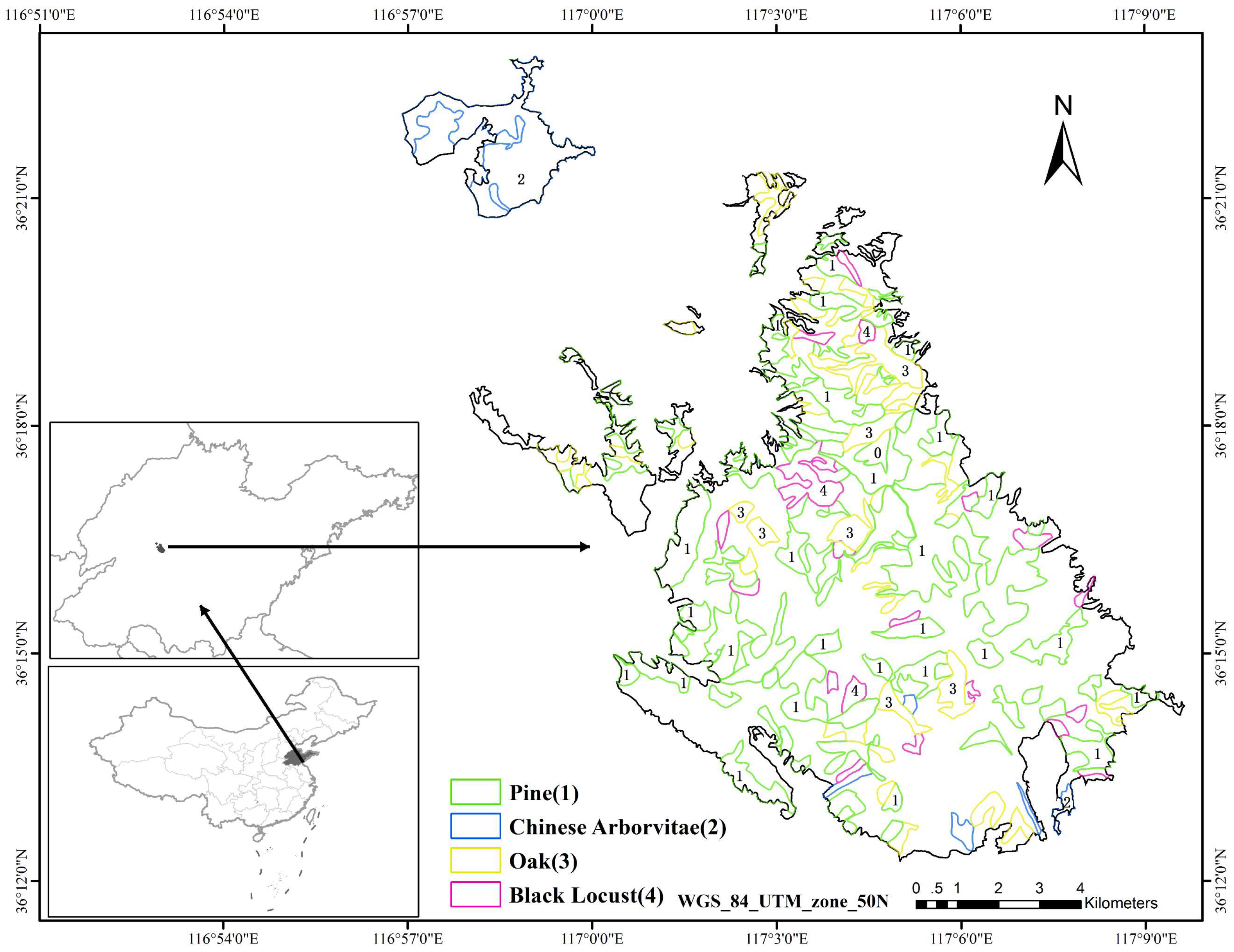
2.1. Study Area

The study area was Mount Taishan, which is located in Tai’an City, Shandong Province, China. The study area was delimited by the boundaries of the Mount Taishan forest farm (Figure 1). Mount Taishan is in the central part of Shandong Province. This area represents one of China’s five great mountainous regions and has an important ecological and cultural status [23]. This region features a warm-temperate semihumid monsoon climate. The climate changes with elevation. The terrain tends to high in the north and west and low in the south and east, and the topography is undulatory, with a height difference between the plain and piedmont of over 1300 m. The forest coverage rate of Mount Taishan is more than 80%, which is mainly composed of plantation and secondary forest, and the proportion of pure forest is 55%. This area features coniferous forest and coniferous-broad-leaved mixed forest, which is typical in warm-temperate mountain areas. The Taishan forest farm, which covers 11,730 ha, was selected as the research area. The main tree species in the study area are pine, Chinese arborvitae (Platycladus orientalis), oak (Quercus) and black locust (Robinia pseudoacacia). Pine can be divided into Pinus tabulaeformis, Pinus thunbergii and Pinus densiflora, and oak can be divided into Quercus acutissima and Quercus variabilis. Pinus tabulaeformis accounts for the largest proportion and is the dominant vegetation species on Mount Taishan. Secondary forests of Pinus tabulaeformis are mainly distributed in the upper part of Mount Taishan. Secondary forests of oak and Chinese arborvitae are mainly distributed in the middle and lower parts of Mount Taishan [24,25].

2.2. Data

2.2.1. Satellite Data

Landsat data is suitable for long-term and large-scale resource exploration. This study used surface reflectance (SR) data from Landsat 8 OLI (Landsat 8 OLI/TIRS surface reflectance) [26] Considering the effects of weather conditions and forest phenology, the data were consistent with the ground survey data. The dates of the images were March 26, 2016, September 2, 2016, October 4, 2016 and November 5, 2016. We chose Landsat 8 bands 2 through 7 for our analysis but focused our efforts on band 4 (red) and band 5 (near-infrared, NIR), as these bands are shown to respond most strongly to surface vegetation conditions (

Table 1. Spectral bands of Landsat 8 used for forest tree species classification.

Name	Units Scale	Wavelength (μm)	Description
Band2	0.0001	0.452–0.512	blue
Band3	0.0001	0.533–0.590	green
Band4	0.0001	0.636–0.673	red
Band5	0.0001	0.851–0.879	near infrared (NIR)
Band6	0.0001	1.566–1.651	shortwave infrared 1 (SWIR1)
Band7	0.0001	2.107–2.294	shortwave infrared 2 (SWIR2)

). The research was based on the implementation of the Google Earth Engine (GEE) platform [27], so all data were accessed on GEE.

2.2.2. Digital Elevation Model

Digital elevation model (DEM) data are important for topographic correction. The Shuttle Radar Topography Mission (SRTM) [28] digital elevation data are an international research effort designed to obtain DEM data on a near-global scale. The SRTM V3 product (SRTM Plus) is provided by NASA JPL at a resolution of 1 arc-second (approximately 30 m). DEM data are the basic data for calculating illumination conditions (ICs), and their accuracy directly affects the topographic correction effectiveness. The slope data and aspect data in the correction model were accessed by calculating the DEM data.

2.2.3. Subcompartment Data

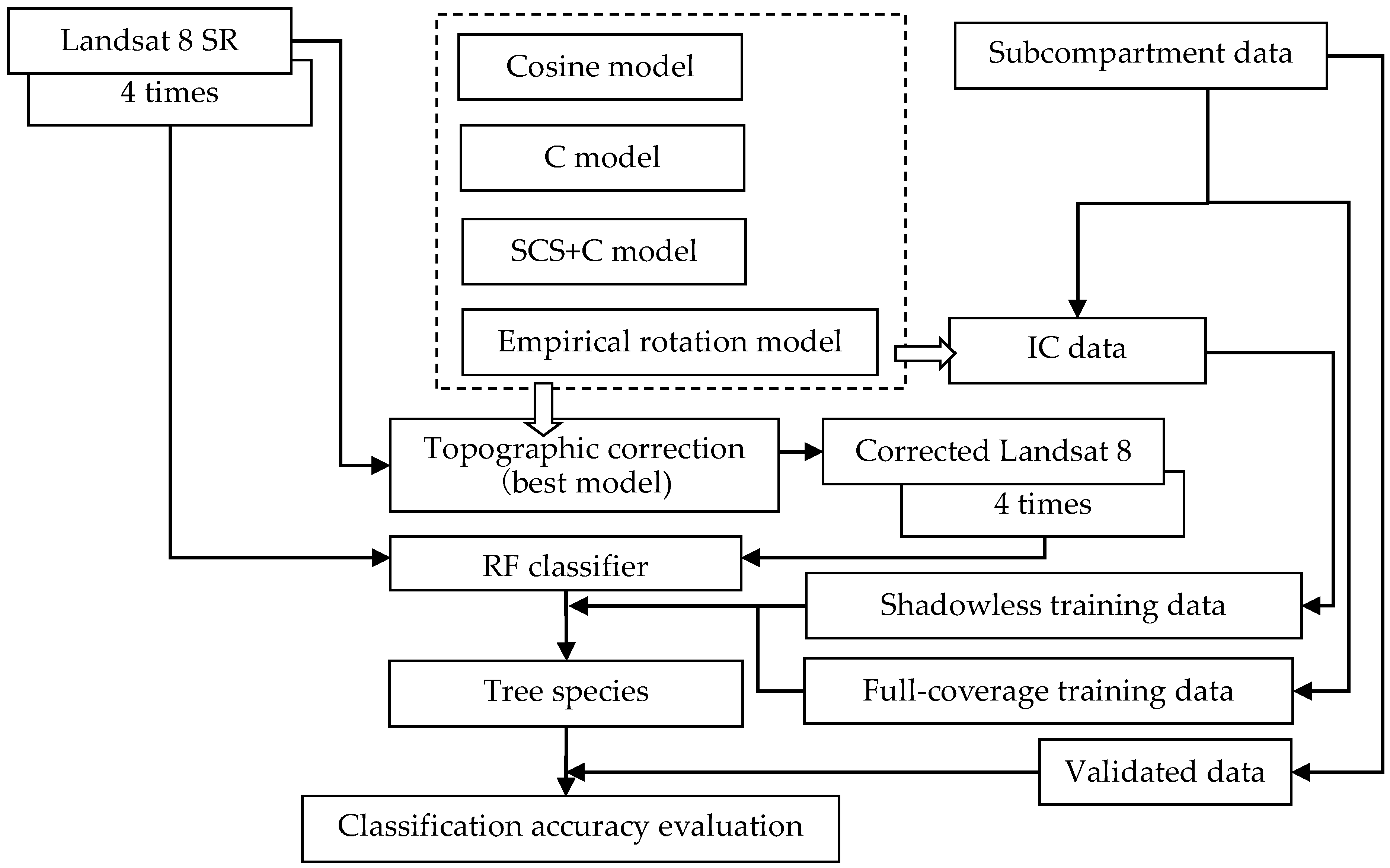
In China, the subcompartment is the basic unit of forest resource protection planning, investigation, statistics and management [29]. The division of subcompartments should be based on obvious topography and object boundaries as much as possible and should take into account the needs for resource investigation and management. Based on the subcompartment map, a field investigation was carried out in this study. The investigation included tree species and other information. In the geographic information system (GIS), the study area is divided into many polygons representing individual, homogeneous forest stands. The investigation results based on the polygon were imported in the form of fields. The subcompartment map used in this study was the result of the 2016 survey, which contains 1713 features and 68 fields. It was provided by the Mountain Tai Management Committee. Field information included tree species, dominant tree species, composition of tree species and other detailed survey data. The tree species field describes the tree species in the subcompartment feature with a tree species code. We can also see whether the subcompartment feature is a single tree species according to the number of tree species codes. There are many coniferous and broad-leaved species in the Mount Taishan region, but pine, oak, Chinese arborvitae and black locust account for the majority of the area. In this study, tree species were divided into these four categories. We created training samples and verification samples based on subcompartment data.

2.3. Methods

2.3.1. Topographic Correction Model

Four commonly used topographic correction models (cosine model [30], C model [31], SCS+C model [32] and empirical rotation model [33]) were used in this study.

Illumination conditions (IC) are the basis of all reflectivity compensation correction models. The IC has a proportional relationship that is determined by the cosine of the angle between the solar zenith and the normal line of the slope, and the model is defined as follows:

$$\cos {\gamma }_i=\cos {\theta }_z\cos {\theta }_s+\sin {\theta }_z\sin {\theta }_s\cos \left({\phi }_z-{\phi }_s\right),$$

(1)

where ${\theta }_z$ is the solar zenith angle, ${\theta }_s$ is the topographic slope angle, ${\phi }_z$ is the solar azimuth angle and ${\phi }_s$ is the slope direction of the topographic surface.

(1) Cosine model:

$${\mathsf{\rho }}_{\mathrm{H}}={\mathsf{\rho }}_{\mathrm{I}}\left(\cos {\mathsf{\theta }}_{\mathrm{z}}∕\cos {\mathsf{\gamma }}_{\mathrm{i}}\right),$$

(2)

where ${\rho }_H$ is the reflectance of the horizontal surface or corrected reflectance, and ${\rho }_I$ is the reflectance of the slope surface, or observed reflectance. The model considers that the correction has nothing to do with the wavelength, underestimating the reflectance of the topographic illumination surface and overestimating the reflectance of the topographic backlight surface, resulting in abnormal values [31].

(2) C model:

$${\rho }_{H\left(\lambda \right)}={\rho }_{I\left(\lambda \right)}\frac{\cos {\theta }_z+C_{\lambda }}{\cos {\gamma }_i+C_{\lambda }}$$

(3)

where ${\mathrm{C}}_{\mathsf{\lambda }}$ is the correction coefficient for the λ band, C = b/a, and a and b are the slopes and intercepts of linear regression calculated between the IC data and this particular band, respectively.

$${\rho }_{I\left(\lambda \right)}=\mathrm{a}\left(\lambda \right)\cos {\gamma }_i+b\left(\lambda \right),$$

(4)

The C model avoids wavelength independence of the cosine model to a certain extent and avoids overcorrection in lower $\cos {\gamma }_i$ value regions.

(3) The SCS+C model:

This is based on the relationship among the sun, canopy and sensor; because tree growth is geotropic, the topography cannot affect the geometric relationship between the sun and the tree. The topography affects the positional relationship between the tree and the surface. The SCS+C model is a model based on the canopy, which enables a change in illumination direction that is more consistent with practice during the process of light canopy correction from sloping to horizontal surfaces. This model is defined as follows:

$${\rho }_{H\left(\lambda \right)}={\rho }_{I\left(\lambda \right)}\frac{\cos {\theta }_z\cos {\theta }_S+C_{\lambda }}{\cos {\gamma }_i+C_{\lambda }},$$

(5)

(4) Empirical rotation model:

The model is defined as follows:

$${\rho }_{H\left(\lambda \right)}={\rho }_{I\left(\lambda \right)}-\mathrm{a}\left(\lambda \right)\ast \left(\cos {\gamma }_i-\cos {\theta }_z\right),$$

(6)

where a is the interception of the band linear regression calculated in Formula (5). This model eliminates the linear dependence of reflectivity on $\cos {\gamma }_i$. The results show that this model can accurately obtain top-of-atmosphere and top-of-canopy reflectivities from Landsat data.

These four models can be used on the GEE platform. Topographic information was obtained by SRTM, and satellite metadata were used to obtain information such as the angle of the satellite on the solar zenith. The ${\mathrm{C}}_{\mathsf{\lambda }}$ parameters used in the model were calculated for each band in Landsat data, which made the models more applicable [34].

2.3.2. Evaluation of the Topographic Correction

The evaluation involved the use of standard deviation (SD) and histograms to evaluate the effectiveness of the topographic correction [35]. First, the SD of all bands before and after correction were counted, and the contrast histogram of the NIR band before and after correction was created. Based on all data from the whole image, the effectiveness of the correction model was evaluated. Then, we chose a reservoir in the study area, which was very obvious in the remote-sensing image, and drew the region of interest to evaluate the stability of the correction model by calculating the reflectance changes before and after correction. Finally, the SDs of the NIR and red bands before and after correction and the correlation coefficients of the NIR band, red band and IC before and after correction were calculated according to each tree species by using the tree species survey data.

2.3.3. Method of Tree Species Classification

Tree species classification includes three parts: topographic correction of multitemporal remote-sensing images, training data production and random forest algorithm classification (Figure 2). First, according to the forest phenology and cloud amount factors, we chose four representative Landsat images. Multiseasonal remote-sensing data help to improve classification accuracy [36]. We use the four methods in the dotted box of Figure 2 to correct the remote-sensing image shadow and create the correction dataset. Then, the training data were created as random points in the pure forest data, which were extracted from the subcompartment data by forest structure fields. The field describes the composition of forest species in the subcompartment data. These data are full-coverage training data. To study the impact of training data distribution on classification, we created shadowless training data that used the shadow region extracted by the IC data to mask the full-coverage training data. We used these training data and a random forest algorithm to train classification models. The random forest algorithm [37] is a machine-learning algorithm that contains multiple decision trees [3,38]. Model training is the process of establishing the relationship between remote-sensing images and tree species labels. Since machine-learning algorithms have overfitting problems, shadowless training data avoid the algorithm, covering up the effectiveness of topographic correction, because the correct classification is based on spectral consistency, not by providing tree species information in shaded areas to the classifier. Finally, the training dataset was used to train the random forest classifier. We use a training model to classify the remote-sensing data.

2.3.4. Evaluation of the Effectiveness of Different Topographic Correction Models on Tree Species Classification

The original data and tree species classification results after correction were visually evaluated, and the accuracy was evaluated based on the validation data. Based on the area size of the subcompartment data, 240 sampling points are generated by using the function of randomly generating points in GIS. A total of 240 sampling points was randomly generated in the study area. Based on subcompartment data and high-resolution Google Earth images, tree species labels were added to the sampling points. Some sampling points were moved to the shaded area to evaluate the impact of the shaded area on tree species classification. To study the influence of topography in topographic correction on tree species classification, we used 1 to subtract the area ratio of correctly classified tree species in the pure forest area to calculate the inconsistency rate, zonal statistics of the inconsistency rate and the IC data, and we drew the distribution histogram of the inconsistency rate and evaluated the relationship between topographic correction and tree species.

3. Results

3.1. Effectiveness of the Topographic Correction Models

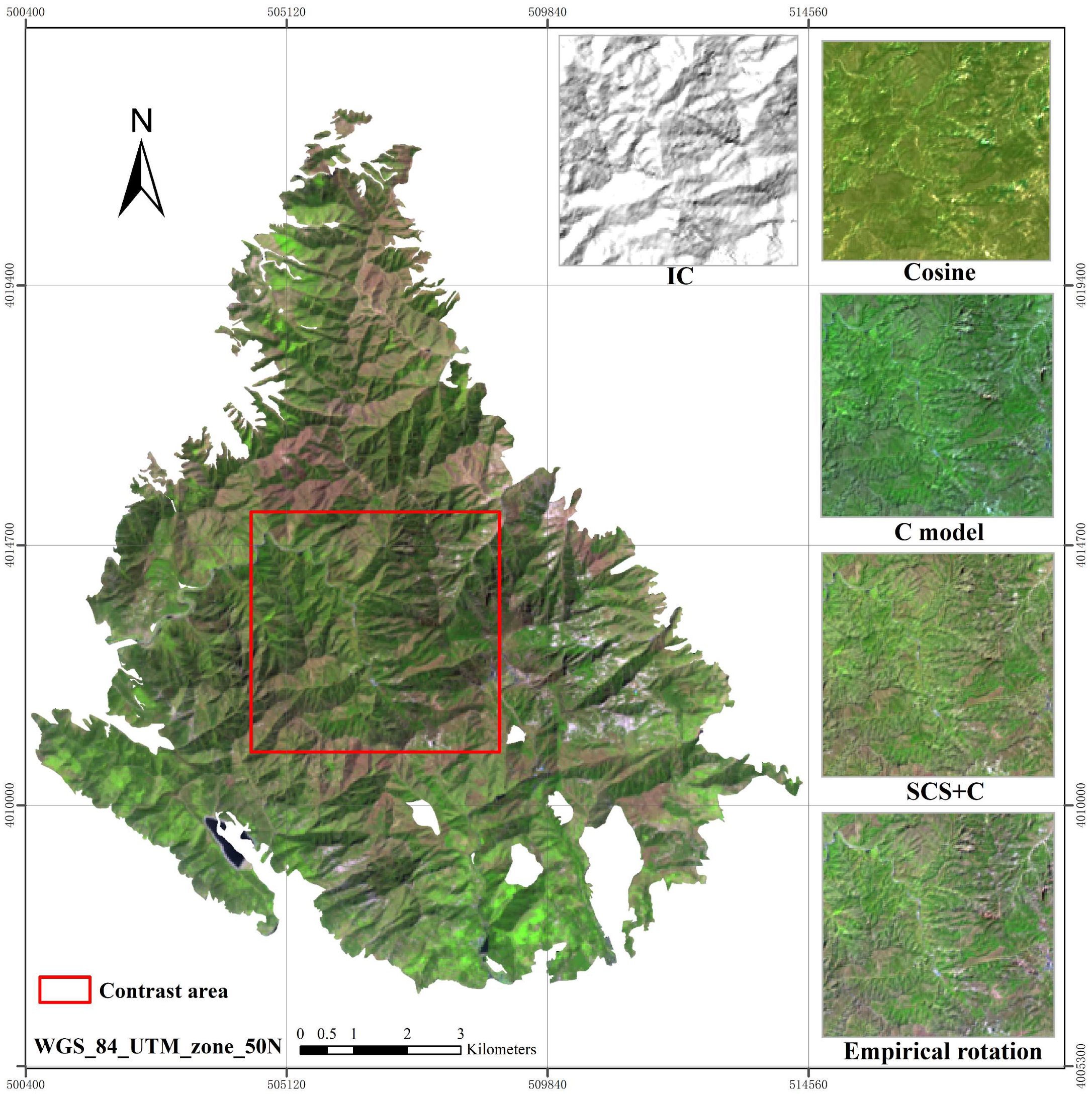
3.1.1. Visual Evaluation of the Topographic Correction

A qualitative evaluation was conducted by visual comparison of the correction effectiveness of the topographic correction model in the study area. The visual comparison is mainly based on three aspects: (1) the effectiveness of removing shadows, (2) whether the color is consistent before and after and whether there is an overcorrection problem and (3) texture features of the images. Through color synthesis, we can see the effect before and after correction (Figure 3). The original reflectance data have three-dimensional characteristics because of topographic fluctuations. IC data can reflect the change in brightness caused by the topographic influence. The comparison of the two pictures demonstrated that the three-dimensional characteristics of the original data were consistent with the change in brightness and shade of the ICs.

All four models can remove most of the topographic shadows and restore the reflectivity information of the shaded areas, which was consistent with the visual impression of adjacent nonshaded areas. The cosine model had many obvious bright spots in the ridge area, which was quite different from the original data and had the problem of overcorrection. There was no obvious overcorrection in the other models. However, after being stretched with SD enhancement, the color depth of the cosine model was found to have decreased, and the color depth of the C model was found to have increased, while the results of the SCS+C model and empirical rotation model were more consistent with and closer to the original data. All images can retain the texture features of objects well, but the corrected images were flatter, and the stereoscopic effect disappeared. Ridges, valleys and other topographic features were difficult to recognize. In summary, from the visual effect, the SCS+C model and empirical rotation model were better than the other models.

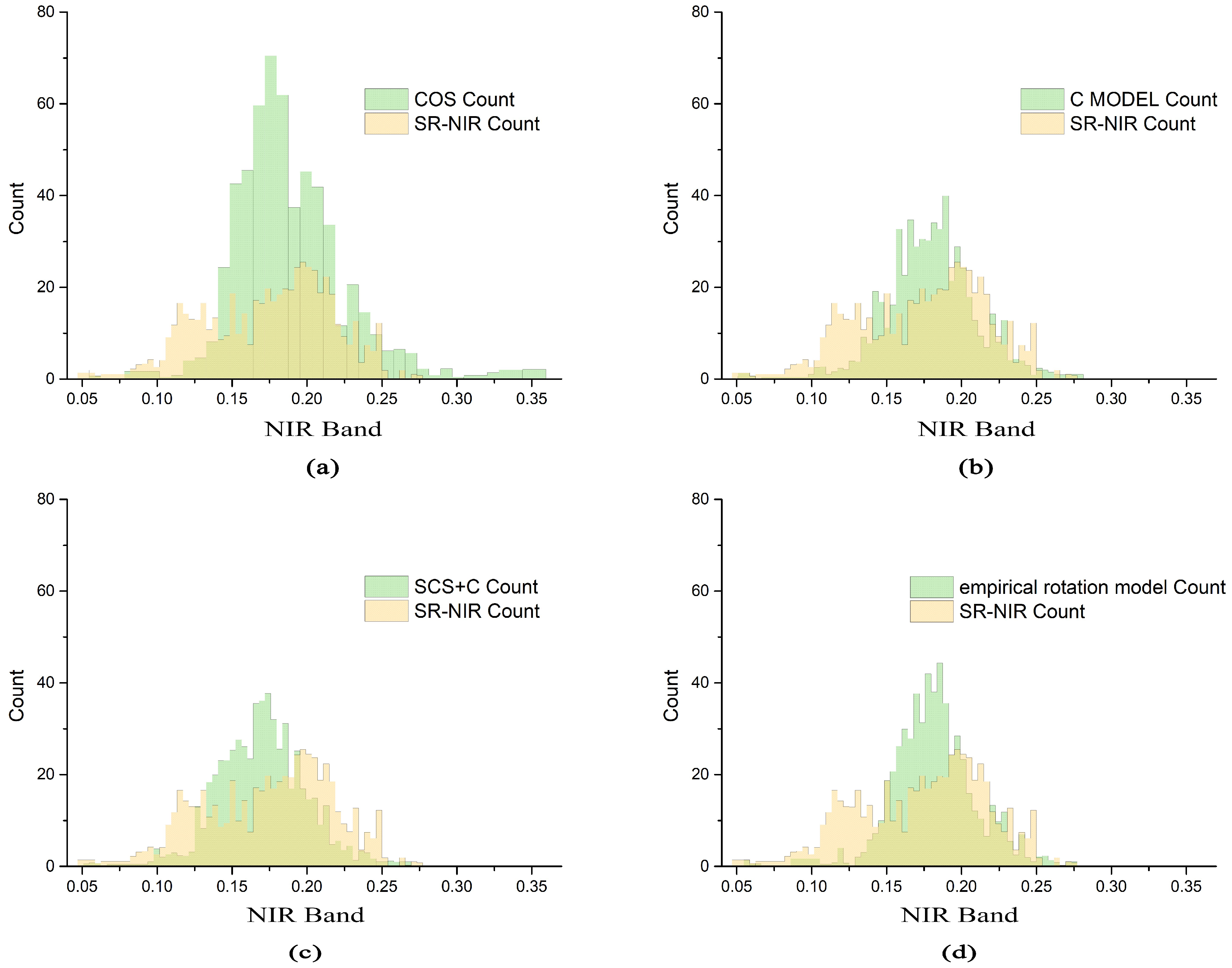
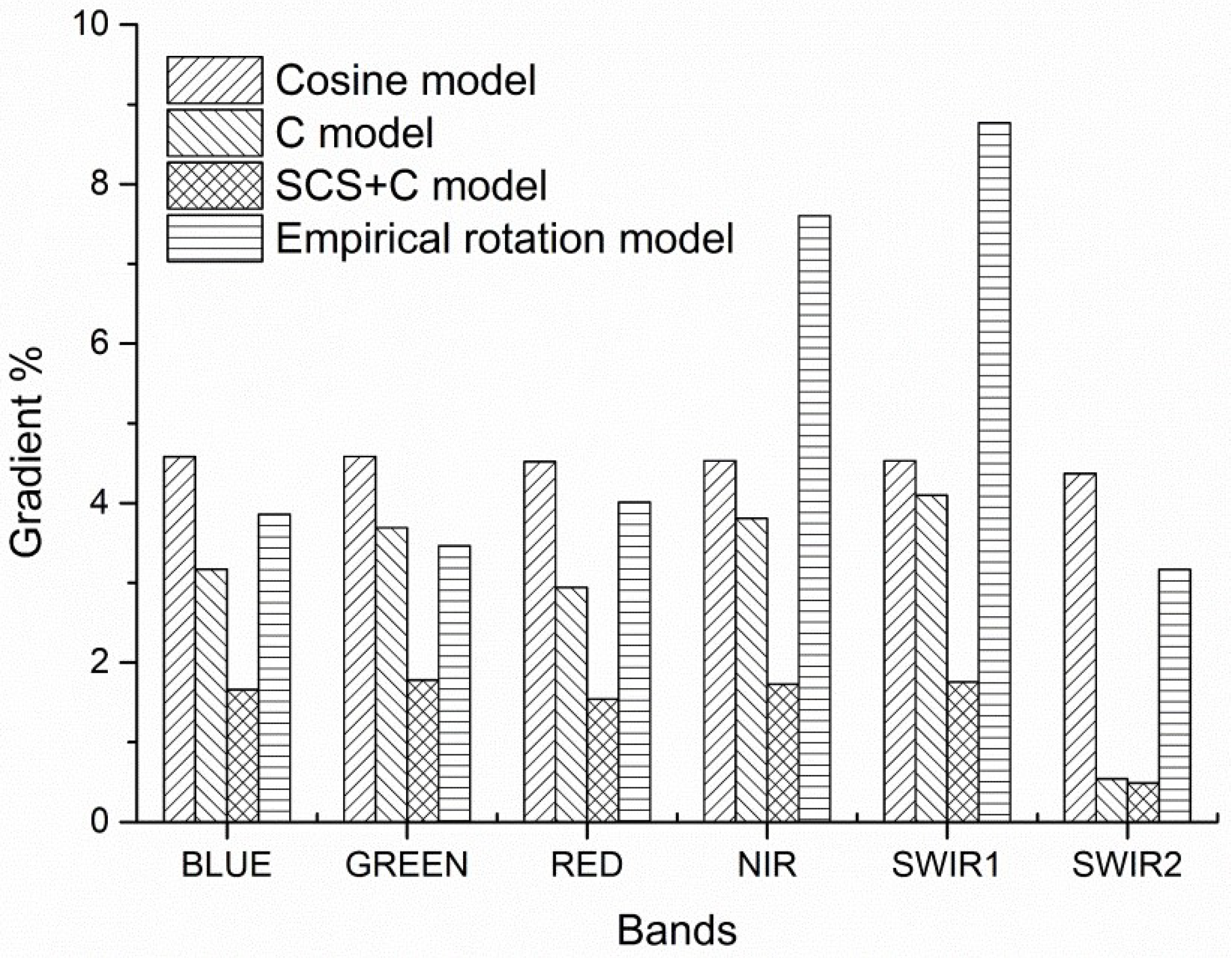
3.1.2. Analysis of Band Information before and after Topographic Correction

The SD reflects the degree of data dispersion. Generally, the spectral value of the same ground feature should be the same, but due to the influence of topography, there will be great variations. We calculated the SD of different bands of the image before and after correction (

Table 2. Standard deviation statistics of spectral bands before and after topographic correction. SR refers to “surface reflectance” and represents precorrected conditions. The model represents the conditions after topographic corrected by the specify model.

	SR	Cosine Model	C Model	SCS+C Model	Empirical Rotation Model
Blue	0.013	0.008	0.009	0.009	0.008
Green	0.016	0.012	0.011	0.011	0.009
NIR	0.042	0.037	0.030	0.029	0.027
Red	0.022	0.014	0.015	0.015	0.013
SWIR1	0.055	0.035	0.040	0.039	0.034
SWIR2	0.044	0.030	0.033	0.032	0.028

). SWIR1 band reflectance data had the largest SD. After correction, the cosine model and empirical rotation model had the best correction effectiveness, and the SDs of the other two models were also reduced. The NIR and red bands are important bands for vegetation monitoring. The smallest SD after the NIR band correction was observed in the empirical rotation model, followed by the SCS+C model and C model, and the worst SD was observed in the cosine model. The empirical rotation model had the smallest SD after the red band correction, and the effectiveness of the four models was very close. All correction models can effectively reduce the SD of each band, and the empirical rotation model (followed by the SCS+C model) was the best in all bands.

The NIR band responds well to the changes in vegetation. We obtained histogram statistics before and after the NIR band correction (Figure 4). The graph shows that the NIR band reflectance histogram of the remote-sensing image did not show a normal distribution due to topographic factors. It formed two peaks: a low value (0.12) and a high value (0.20). This showed that due to the influence of topographic slope and slope direction, some pixels received insufficient illumination, while the other parts showed a saturation trend. After the treatment of the four correction models, the NIR band histogram showed an approximate normal distribution, which was consistent with the random features of natural phenomena, showing the reflection characteristics of objects in the real state. In the four models, the cosine model greatly compressed the original data, gathered many values in the 0.15–0.2 reflectivity region and the left and right sides were not completely symmetrical. There were also data outside the original range, which was considered to be the result of overcompressing. Compared with the C model, the SCS+C model had the same area with values higher than 0.2. In the range of 0.12–0.17, the SCS+C model was smoother, which was related to the canopy correction rather than the topographic correction of the SCS+C model. The empirical rotation model was smooth on both sides of the peak. Compared with the former two models, the reflectance distribution was concentrated at the peak. All models can correct the NIR band reflectivity to approximate a normal distribution. In terms of comprehensive distribution morphology, continuity and deformation, the SCS+C model and empirical rotation model had better correction effectiveness.

3.1.3. Effectiveness of Topographic Correction on Tree Species Reflectivity

Based on forest species composition information in pure forest data, we counted the SD changes for pine, Chinese arborvitae, oak and black locust in the NIR and red bands before and after correction, respectively (Figure 5). When we examined a single tree species, the SD of the cosine model increased, and the pine species stretched abnormally in the NIR band. The empirical rotation model reduced the SDs of all tree species. When we examined pines, the SD of the blue, green and red bands of the C model was higher than the original SD of reflectance. The SD of the SCS+C model-corrected image was higher than the original SD in the blue band for pines and the red band for oak. Statistical results showed that different correction models had different effects on different tree species, which was related to the distribution of tree species and the inconsistencies in the reflections of different bands. The empirical rotation model was very stable, and the SD of all bands of all tree species was less than the original SD of reflectance. The second-best results were obtained by the SCS+C model.

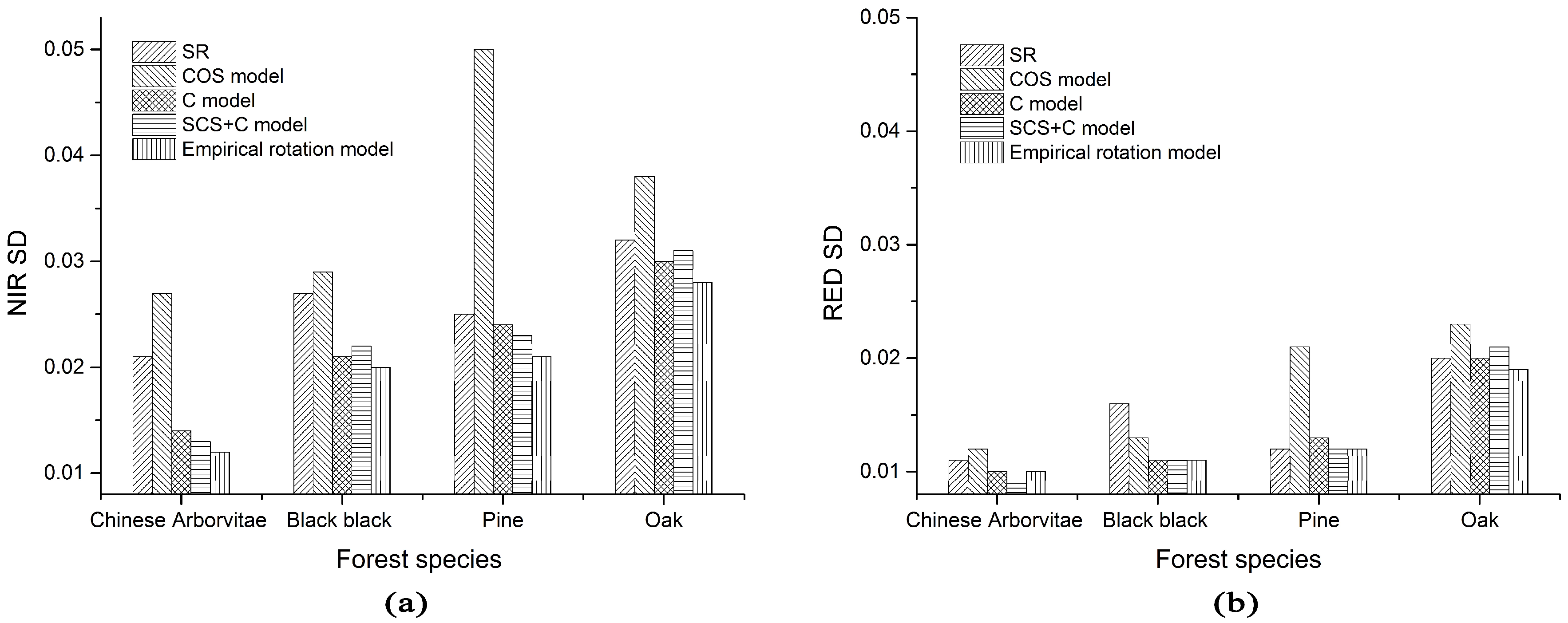
3.1.4. Stability Analysis of Topographic Correction

Changes in the water body reflectance can be used to evaluate the validity of a topographic correction model by statistical comparisons of this reflectance before and after correction has been applied to the study area (Figure 6). Water bodies are horizontal, so the topographic correction model should not have a large impact on them. The change in reflectance of all models was less than 10%, and the change in the SCS+C model was the smallest, at less than 2%. The empirical rotation model is an experience-based rotation model. Compared with other models, the reflectivity of the water surface changed greatly, especially in the NIR and short-wavelength infrared (SWIR) bands. The changes induced by the other two correction models were between 3% and 5%.

In summary, compared with the other two models, the cosine model and C model did not perform as well in terms of the correction effectiveness and stability. Therefore, the SCS+C model and empirical rotation model were the main models used in the further study of tree species classification.

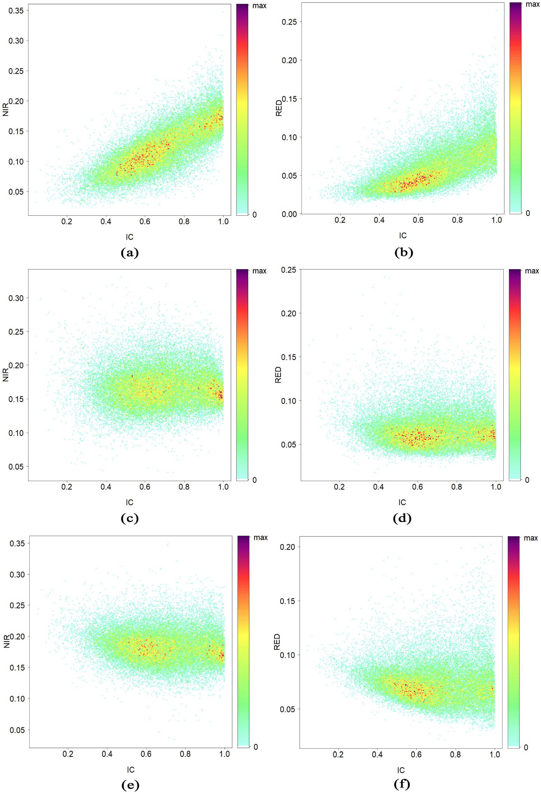
3.1.5. Analysis of Correlations among the IC, NIR Band and Red Band of Different Tree Species before and after Correction

The tree species distributed in the shaded area will affect the remote-sensing image, resulting in a correlation between the remote-sensing spectral value and topography. We used the tree species information of subcompartment data to calculate the correlation between the remote-sensing spectral value and the IC value in the region (

Table 3. Correlation coefficient of spectral band and illumination conditions (IC) before and after correction in the NIR band and red band. SR represents the coefficient before correction, SCS+C represents the coefficient after correction by SCS+C model, and empirical rotation represents the coefficient after correction by the empirical rotation model.

Tree Species	NIR			Red
	SR	SCS+C	Empirical rotation	SR	SCS+C	Empirical rotation
Pine	0.58	0.79 × 10−3	0.15 × 10−1	0.43	0.28 × 10−3	0.77 × 10−2
Chinese arborvitae	0.69	0.13 × 10−1	0.24 × 10−2	0.29	0.22	0.22
Oak	0.41	0.94 × 10−2	0.61 × 10−2	0.30	0.33 × 10−2	0.58 × 10−3
Black locust	0.47	0.80 × 10−5	0.85 × 10−2	0.44	0.13 × 10−2	0.60 × 10−3

). Before correction, both the NIR and red bands of the image had a high correlation with the IC. The highest correlations were observed in the NIR bands of pines and Chinese arborvitae, which were 0.58 and 0.69, respectively. The lowest correlations were found for the red bands of Chinese arborvitae and oak, which were 0.29 and 0.30, respectively. The correlation of the NIR band was higher than that of the red band. The correlation coefficients of pines and Chinese arborvitae after SCS+C correction were lower than those of the empirical rotation method, whereas those of oak exhibited the opposite pattern. For black locust, the SCS+C model was better than the empirical rotation model in the NIR band, and vice versa in the red band. The correlation reflects the degree of influence of the topography on the spectral reflectance of trees. Except for the red band of Chinese arborvitae, the correlation of the NIR band and red band of all tree species was significantly reduced by the models.

By constructing density plots between the IC dataset and the individual bands for pine, we can better understand the process of spectral value processing of the topographic correction method (Figure 7). As shown in the Figure 7, IC values of 0.3–1.0 were distributed over a large area. The original reflectance data were highly correlated with the IC values. After correction, the correlation coefficient between reflectance and IC was significantly reduced. As shown in the Figure 7, both the SCS+C model and empirical rotation model rotated the reflectance distribution of the original data from tilted to nearly horizontal, while the empirical rotation model rotated the distribution only on the basis of the original data, and its interior distribution was very close to that of the original data. The distribution of points in the scatter plot for the SCS+C model changed obviously to different degrees. In the NIR band, the density of red points with high densities was reduced after correction with the SCS+C model. The red band exhibited clear changes: the empirical rotation model rotated the data as a whole, while the SCS+C model transformed one density center into two distinct density centers. Due to the relatively small distribution area of other tree species, the rotation changes were not obvious.

3.2. Topographic Correction Effectiveness on Tree Species Classification

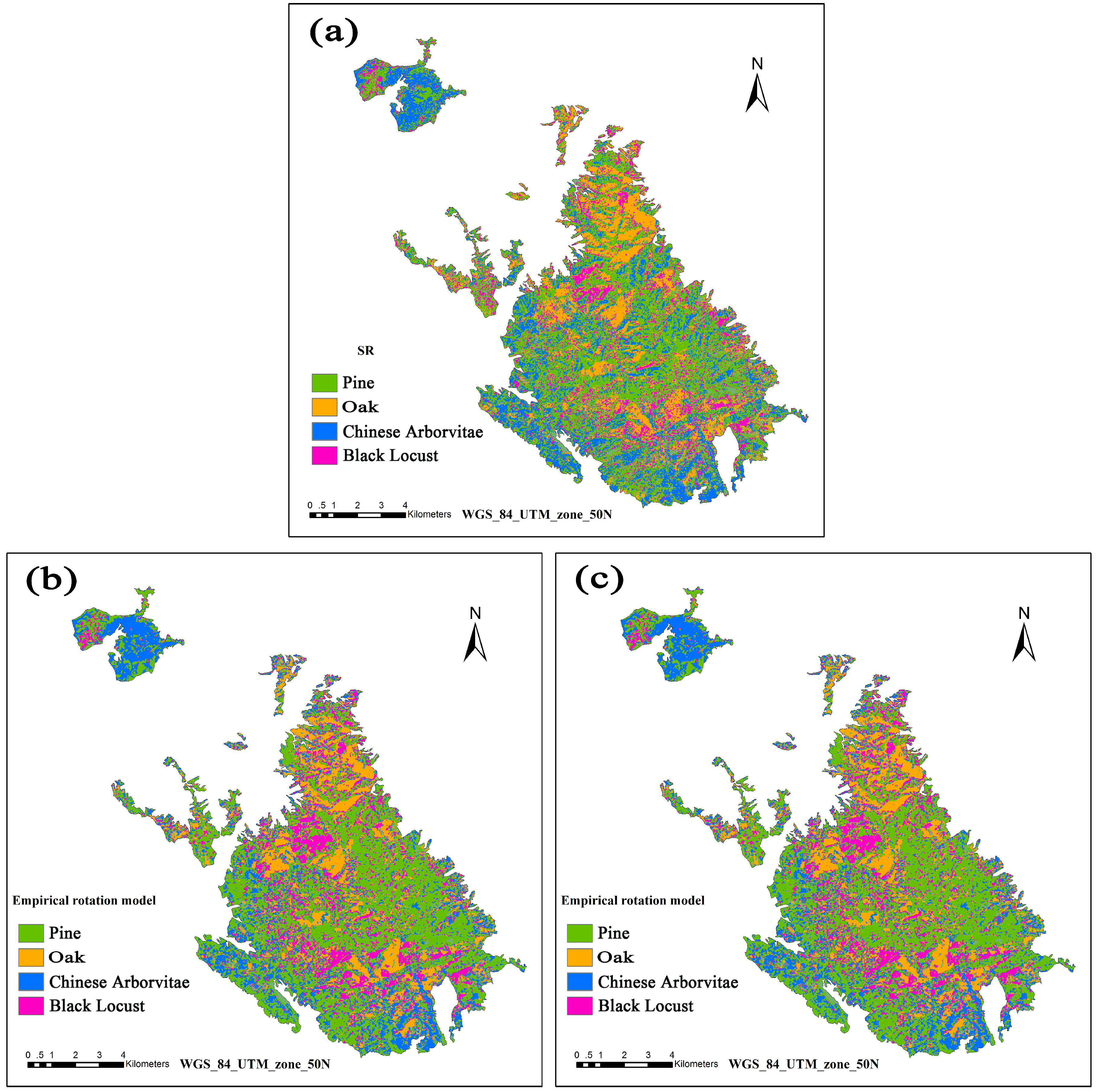
3.2.1. Classification Results of Tree Species and Accuracy Evaluation

Whether the training data were covered with shaded areas had a great impact on the accuracy of the classification results (

Table 4. Classification accuracy with different training data. SR represents the data before correction, and SCS+C model and empirical rotation model represent the data after correction.

Shadowless Training Data	Overall Accuracy	Kappa	Full-Coverage Training Data	Overall Accuracy	Kappa
SR	0.65	0.52	SR	0.76	0.68
SCS+C model	0.74	0.67	SCS+C model	0.79	0.73
Empirical rotation model	0.72	0.64	Empirical rotation model	0.77	0.70

). The classification results of the full-coverage training data showed little difference in terms of accuracy before and after correction; the SCS+C model performed better, and the empirical rotation model showed slightly improved accuracy. The classification results of shadowless training data had great differences before and after topographic correction. The SCS+C model performed the best, and its accuracy was 13% higher than that before correction. The performance of the empirical rotation model also improved significantly. Due to the inconsistency in the reflectance of the original data in the shaded area, the accuracy was low. Therefore, when the survey data in the study area are comprehensive, the influence of topography can be avoided to some extent by including training sample points in shaded areas; when the amount of data in the study area is not adequate, the classification must rely on visual or partial data, and the topographic correction of the data should be included in the pretreatment step to improve the classification accuracy.

The random forest algorithm was used to classify the data before and after correction, and maps of the resulting forest species distribution were created. As shown in Figure 8, Chinese arborvitae is mainly distributed in the northwestern and southern parts of Mount Taishan. Oak species are mainly distributed in the northern part of Mount Taishan, while a small amount is distributed in the central and southern parts. Black locust covers the least area, and the distribution is fragmentary. Pines are widely distributed throughout the whole area. The Landsat 8 data corrected by the four models can effectively distinguish among these four tree species, but the classification results of the four models differed in terms of specific distributions due to the different corrections of each model (

Table 5. Area statistics derived from classification of the tree species. SR represents the data of the precorrected data classification results. The SCS+C model and empirical rotation model represent the data after topographic correction. The gradient represents the change rate between the before and after correction data.

Tree Species	SR	SCS+C		Empirical Rotation
	Area (m2)	Area (m2)	Gradient (%)	Area (m2)	Gradient (%)
Pines	57,028	58,647	2.84	58,981	3.424
Chinese arborvitae	27,515	26,101	−5.14	26,779	−2.67
Oak	21,438	22,631	5.56	21,801	1.69
Black locust	18,987	18,376	−3.22	20,535	8.15

).

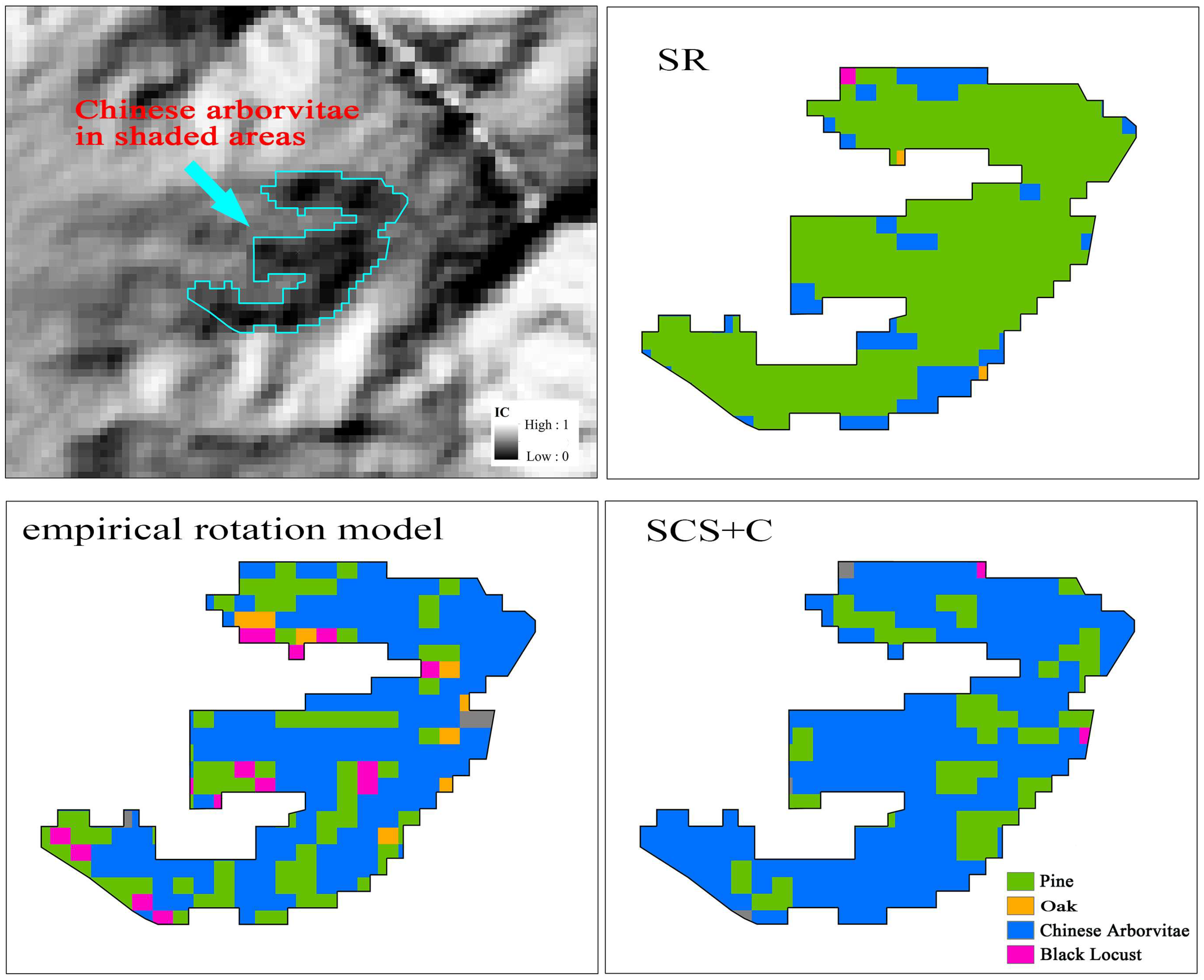
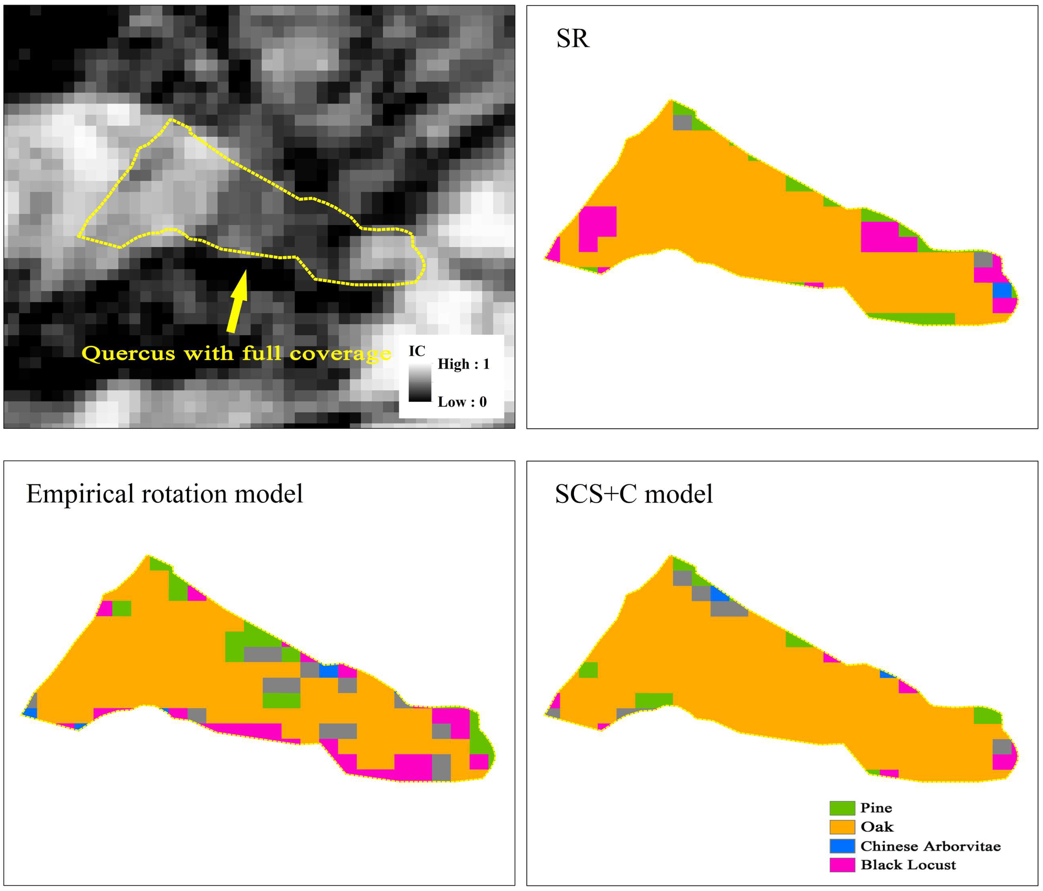
3.2.2. Topographic Correction Effectiveness on Tree Species Classification in Shaded Areas

The tree species in the area with low ICs were entirely composed of Chinese arborvitae (Figure 9). In the original SR data classification results, most of these trees were identified as pine species and only the edges were identified as Chinese arborvitae. However, after correction, both the SCS+C model and empirical rotation model correctly recognized most of the species as Chinese arborvitae by recovering their reflectivities. Even so, there were still some errors in the two correction models. On the one hand, the spectral characteristics of these two tree species are similar, which can easily lead to errors. On the other hand, although the correction maintains the spectral information in shaded areas, the information recovery is not complete due to DEM error and the influence of the distribution of the vegetation itself. Complete restoration is only an ideal situation.

The classification results for oak were slightly different from those for Chinese arborvitae. The original data can be better distinguished by using training sample points in no-shadow areas. Even in areas with low illumination values, the classification accuracy of oak was high (Figure 10). The reason is that the spectral characteristics of oak are quite different from those of pine and Chinese arborvitae and are therefore easy to distinguish. After the correction, the results of the SCS+C model were better than those of the original image. After correction by the empirical rotation model, oak was easily distinguished, and a few areas were recognized as other tree species.

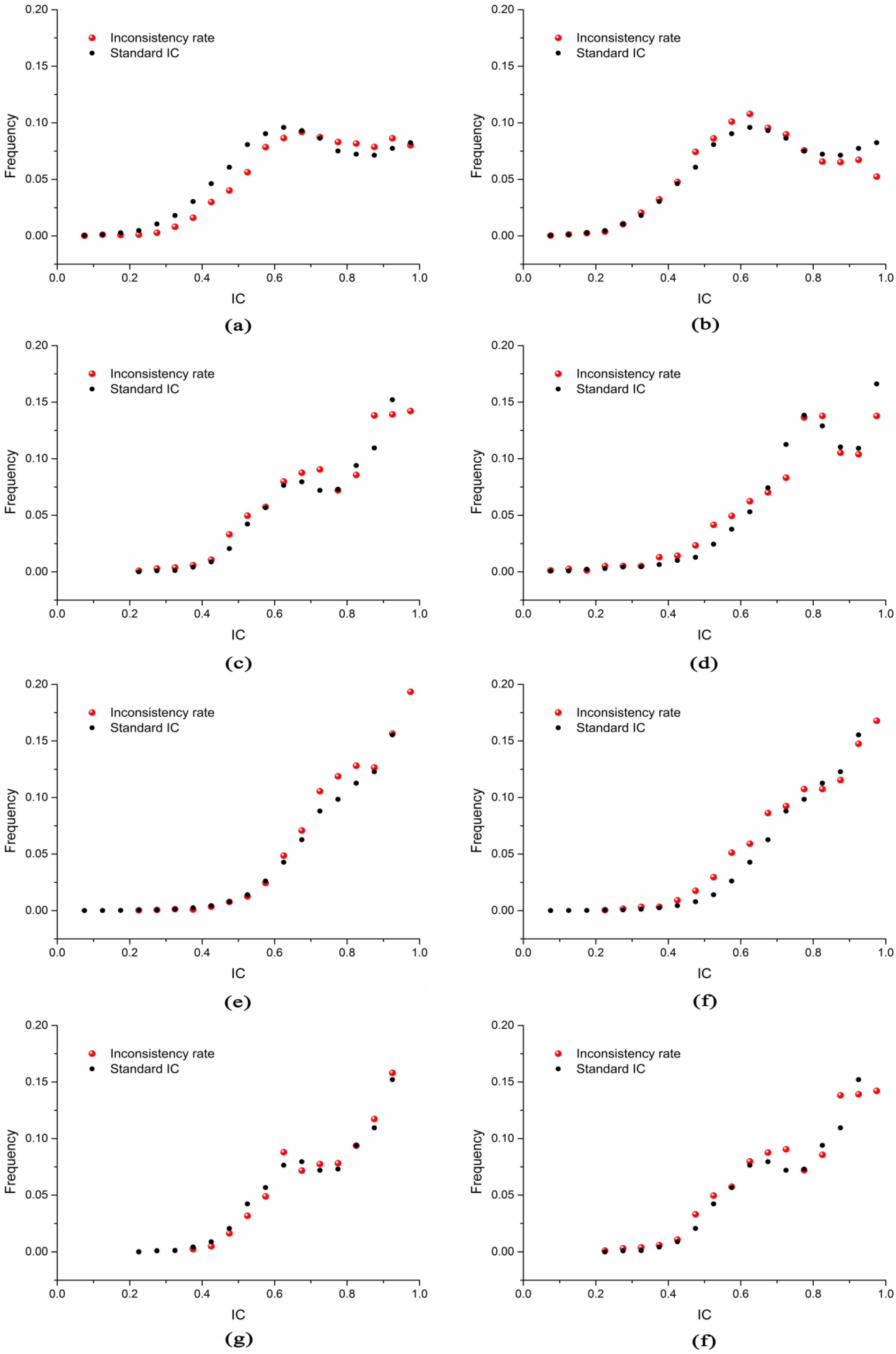
3.2.3. Effect of Topographic on Classification Inconsistency Rate

The black symbols in Figure 11 are the normalized values of the area of tree species in pure forests in different intervals of the IC. The four types of tree species had different topographic distributions based on observation of the standard IC distribution. Pine had two peaks at IC values of 0.6 and 1.0. Black locust had similar peaks at IC values of 0.6 and 0.9. Chinese arborvitae and oak were mostly distributed in the IC range of 0.8–1.0. The red symbols in Figure 11 show the inconsistency rate of tree species classification results by remote sensing. After correction, the inconsistency rate of interval 0.4–0.6 increased and that of interval 0.7–0.9 decreased. After correction, the inconsistency rate of Chinese arborvitae increased in the 0.5–0.7 interval and decreased in the 0.9–1.0 interval. After correction, the inconsistency rate of oak increased in the 0.4–0.7 interval and decreased in the 0.7–0.9 interval. The inconsistency rate of black locust increased from 0.7 to 0.8 after correction. The inconsistency rate of pine changed greatly after correction and was greatly affected by correction. Black locust showed the opposite result. The relationship between the inconsistency rate and IC was determined by the combination of tree species and their topographic distributions. Topographic correction mainly reduced the inconsistency rate in the 0.4–0.6 interval. Obviously, the correction model maintained the reflectance information of the low IC area throughout the correction, but the model also introduced uncertainty in the classification of the high illumination area.

4. Discussion

Topographic correction can reduce the effects of varying topography/terrain surfaces and associated shadowing on spectral reflectance. Although there is no effective method to completely remove this effect, researchers have attempted to improve the effectiveness of topographic correction using various methods. The influence on the topographic correction effectiveness is controlled mainly by the selection of the correction model and the accuracy of the DEM. At present, none of the models can fully explain the relationship between the illumination coefficient and the band reflectivity. Of the four models discussed in this study, the cosine model is a simple optical function, the C model is used to calculate the empirical relationship between the band reflectance and illumination coefficient, the SCS+C model considers the relationship between the sun canopy and sensor and uses the C model to avoid overcorrection and the empirical rotation model eliminates the linear relationship between the band reflectance and illumination coefficient. Although these models all achieve the effectiveness of topographic correction, they are not able to remove all illumination differences resulting from topographic variability. This requires more in-depth research to find a model that fully explains the relationship between reflectivity and the care factor.

The accuracy of the DEM data is another aspect that has a great influence on the correction effectiveness. In the topographic correction model, the illumination coefficient is an important parameter. The IC is calculated based on the slope and aspect, and the slope and aspect are calculated based on the DEM. Thus, the accuracy of the DEM has a great influence on the parameters of the topographic correction model. In this study, we used the elevation data provided by the SRTM, which has a spatial resolution of 30 m. We also used the data of TanDEM-X 90 m for comparison [39]. For TanDEM-X, the overall accuracy and kappa coefficients of the classification results increased by 0.03–0.08 and 0.03–0.09, respectively, but the accuracy of the empirical rotation model results decreased. Since TanDEM-X only obtains 90-m resolution data, the IC calculation involves both slope and aspect. In addition to elevation, horizontal distance is also needed in the calculation. Hence, the spatial resolution affects the accuracy. Although there is no in-depth study on how the DEM accuracy affects the classification accuracy, the higher the DEM accuracy is, the better the correction effectiveness. If the area is small, we can use photogrammetry technology to generate a more accurate surface. We believe that if we can obtain accurate ground data, the topographic correction effectiveness will be greatly improved. Topographic correction adjusts the value and distribution of the band reflectance according to the relationship between the band reflectance and IC. After the four models are corrected, the SD of the band reflectivity can be reduced. However, according to the histogram, the cosine model with different methods has greatly changed the distribution of the band histogram, while the changes associated with the other three models are more moderate. The difference in the histogram after correction is the difference in the interpretation of the band reflectance and the illumination coefficient by the correction method. Different topographic correction models produced different patterns (Section 3.1.5). In the density maps rotated by the topographic correction models, the overall structure of the graph has not changed, which shows that the models are based on the IC and adjust the spectral values in a predictable fashion. Small changes in the form of different shapes and centers are evident after adjustment. This is because both the SCS+C model and the empirical rotation model use coefficients derived from IC data and band regression. In this way, the model adaptability is good, but there are also problems. This regression value is only an empirical value, and there is great uncertainty. The topographic corrections affect different bands differently, and the empirical coefficients of different bands calculated by the C model can eliminate this difference. The empirical rotation model uses the slope, and the SCS+C model uses the slope and intercept.

The distribution of training data and topographic distribution of tree species also affects the accuracy of tree species classification. The spectra of objects in the shaded area definitely vary; thus, training our model with this knowledge will certainly improve the classification accuracy. However, this will also increase the uncertainty, as it may make the spectral values of a feature close to those of other features. Therefore, the selection of training samples is always a process of regional applicability. This is also demonstrated by the influence of the distribution of tree species on the accuracy of tree species classification. Different species have different IC intervals with good correction effects. This may be related to the spectral reflection, canopy structure or canopy direction of the tree species. However, the influence on the spectral reflectance of different tree species is more complicated. It is not always possible to retain all the information. The best way is to eliminate the impact of the topography. In fact, ratio indexes such as the normalized difference vegetation index (NDVI) can eliminate the influence of topography [40,41]. However, the influence of topography on the spectral band is not completely consistent, so we think that, although the index can reduce the influence, it cannot completely eliminate the influence in the same way that system error can be eliminated. It is necessary to correct the band reflectance. When we perform quantitative research on the band reflectance, we want to know the absolute value of the band reflectance rather than the relative value. This value may be more useful in revealing the influence of topography on the features.

5. Conclusions

Based on Landsat 8 data, we developed four topographic correction models on the GEE platform, and their effectiveness on forest tree species classification were compared in detail. The SCS+C model and empirical rotation model were the best models in terms of visual effects, reducing band SD and adjusting the reflectance distribution. The empirical rotation model had the best effect on reducing the SD of the tree species in the NIR and red bands, while the SCS+C model had a high level of consistency with the original scatter density in adjusting the correlation between the NIR and red bands and the IC. All of the corrected images were associated with improved tree species classification accuracy. When using the full-coverage training areas, the accuracy increased by 4%, and when using the shadowless training area, the total accuracy of the SCS+C model increased by nearly 13%. The inconsistency rate distribution histogram showed that the relationship between the inconsistency rate and the IC was determined by the comprehensive effect of tree species and topographic distribution. When forest species were concentrated in the IC interval of 0.4–0.6, the inconsistency rate decreased significantly after correction, whereas with increasing IC values, the inconsistency rate increased. In other words, the corrected image significantly improved the quality and maintained the reflectance information of the shaded area. This technique can be used as a pretreatment method for forest species classification in mountain areas.

The change in the reflectance of forest areas shaded by topography is the result of complex and multifactor interactions, so it is difficult to maintain an exact value with a single mathematical model. The DEM data used in this study have a resolution of 30 m. In this study, it was found that there were some dislocations between the DEM data and the remote-sensing data. Although the effect can be reduced by resampling, DEM data with higher accuracy should provide better topographic correction results. In addition, the complexity of the ground objects is another factor affecting the topographic correction. The uncertainty in the mixed pixels caused by the 30-m resolution of the Landsat data also led to a reduction in the classification accuracy.

In this study, the effectiveness of four commonly used topographic correction models on tree species classification were analyzed. This work provides a basis for the use of satellite data topographic correction in tree species classification. In future research, we will seek a more accurate model and a more accurate DEM to eliminate the influence of the topographic to the greatest extent. The application of topographic correction can produce more consistent spectral characteristics of ground objects, reduce misclassifications and improve the accuracy of forest tree species investigations, which are very important for the promotion of forest resource investigation methods using remote sensing.

References

1. Scott, C.T.; Köhl, M.; Schnellbächer, H.J. A comparison of periodic and annual forest surveys. For. Sci. 1999, 45, 433–451. [Google Scholar]
2. Immitzer, M.; Atzberger, C.; Koukal, T. Tree species classification with random forest using very high spatial resolution 8-band worldview-2 satellite data. Remote Sens. 2012, 4, 2661–2693. [Google Scholar] [CrossRef] [Green Version]
3. Yu, Y.; Li, M.Z.; Fu, Y. Forest type identification by random forest classification combined with spot and multitemporal Sar data. J. For. Res. 2018, 29, 1407–1414. [Google Scholar] [CrossRef]
4. Ke, Y.; Quackenbush, L.J.; Im, J. Synergistic use of quickbird multispectral imagery and lidar data for object-based forest species classification. Remote Sens. Environ. 2010, 114, 1141–1154. [Google Scholar] [CrossRef]
5. Iizuka, K.; Tateishi, R. Estimation of CO2 sequestration by the forests in Japan by discriminating precise tree age category using remote sensing techniques. Remote Sens. 2015, 7, 15082–15113. [Google Scholar] [CrossRef] [Green Version]
6. Kozoderov, V.V.; Dmitriev, E.V.; Melnik, P.G.; Donskoi, S.A. Evaluation of the species composition and the biological productivity of forests based on remote sensing data with high spatial and spectral resolution. Izv. Atmos. Ocean. Phys. 2018, 54, 1374–1380. [Google Scholar] [CrossRef]
7. Liu, A. Study on the Theory and Method of Annual Monitoring of Forest Resources. Ph.D. Thesis, Nanjing Forestry University, Nanjing, China, 2006. [Google Scholar]
8. Yu, X.Y.; Zhao, G.X.; Chang, C.Y.; Yuan, X.J.; Heng, F. Bgvi: A new index to estimate street-side greenery using baidu street view image. Forests 2019, 10, 3. [Google Scholar] [CrossRef] [Green Version]
9. Lu, D. Integration of vegetation inventory data and Landsat Tm image for vegetation classification in the Western Brazilian Amazon. For. Ecol. Manag. 2005, 213, 369–383. [Google Scholar] [CrossRef]
10. Schuck, A.; Päivinen, R.; Häme, T.; Van Brusselen, J.; Kennedy, P.; Folving, S. Compilation of a European forest map from Portugal to the Ural Mountains based on earth observation data and forest statistics. For. Policy Econ. 2003, 5, 187–202. [Google Scholar] [CrossRef]
11. Immitzer, M.; Vuolo, F.; Atzberger, C. First experience with Sentinel-2 data for crop and tree species classifications in Central Europe. Remote Sens. 2016, 8, 166. [Google Scholar] [CrossRef]
12. Grabska, E.; Hostert, P.; Pflugmacher, D.; Ostapowicz, K. Forest stand species mapping using the Sentinel-2 time series. Remote Sens. 2019, 11, 1197. [Google Scholar] [CrossRef] [Green Version]
13. Chiang, S.-H.; Valdez, M. Tree species classification by integrating satellite imagery and topographic variables using maximum entropy method in a Mongolian forest. Forests 2019, 10, 961. [Google Scholar] [CrossRef] [Green Version]
14. Vanonckelen, S.; Lhermitte, S.; Van Rompaey, A. The effect of atmospheric and topographic correction methods on land cover classification accuracy. Int. J. Appl. Earth Obs. Geoinf. 2013, 24, 9–21. [Google Scholar] [CrossRef] [Green Version]
15. Moreira, E.P.; Valeriano, M. Application and evaluation of topographic correction methods to improve land cover mapping using object-based classification. Int. J. Appl. Earth Obs. Geoinf. 2014, 32, 208–217. [Google Scholar] [CrossRef]
16. Zhu, X.Y.; Sun, M.W.; Wang, S.G.; Yu, L.; Chen, Q.; Wang, Y. Correction of false topographic perception phenomenon based on topographic correction in satellite imagery. IEEE Trans. Geosci. Remote Sens. 2017, 55, 468–476. [Google Scholar] [CrossRef]
17. Galvao, L.S.; Breunig, F.M.; Teles, T.S.; Gaida, W.; Balbinot, R. Investigation of terrain illumination effects on vegetation indices and Vi-derived phenological metrics in subtropical Deciduous forests. Gisci. Remote Sens. 2016, 53, 360–381. [Google Scholar] [CrossRef]
18. Vazquez-Jimenez, R.; Romero-Calcerrada, R.; Ramos-Bernal, R.N.; Arrogante-Funes, P.; Novillo, C.J. Topographic correction to Landsat imagery through slope classification by applying the Scs plus C method in mountainous forest areas. ISPRS Int. J. Geo Inf. 2017, 6, 287. [Google Scholar] [CrossRef]
19. Ghasemi, N.; Mohammadzadeh, A.; Sahebi, M.R. Assessment of different topographic correction methods in alos Avnir-2 data over a forest area. Int. J. Digit. Earth 2013, 6, 504–520. [Google Scholar] [CrossRef]
20. Pimple, U.; Sitthi, A.; Simonetti, D.; Pungkul, S.; Leadprathom, K.; Chidthaisong, A. Topographic correction of Landsat Tm-5 and Landsat Oli-8 imagery to improve the performance of forest classification in the mountainous terrain of Northeast Thailand. Sustainability 2017, 9, 258. [Google Scholar] [CrossRef] [Green Version]
21. Szantoi, Z.; Simonetti, D. Fast and robust topographic correction method for medium resolution satellite imagery using a stratified approach. IEEE J. Sel. Top. Appl. Earth Obs. Remote Sens. 2013, 6, 1921–1933. [Google Scholar] [CrossRef]
22. Ba, A.; Laslier, M.; Dufour, S.; Hubert-Moy, L. Riparian trees genera identification based on leaf-on/leaf-off airborne laser scanner data and machine learning classifiers in Northern France. Int. J. Remote Sens. 2020, 41, 1645–1667. [Google Scholar] [CrossRef]
23. Liu, S.; Peng, G.; Panwei, L.; Xiang, N.; Bing, W. An ecosystem services assessment of Tai mountain. Acta Ecol. Sin. 2017, 37, 3302–3310. [Google Scholar]
24. Lian, X. Study on Natural Regeneration and Sapling Distribution of Platycladus Orientalis Plantation in Mount Tai. Master’s Thesis, Shandong Agricultural University, Shandong, China, 2014. [Google Scholar]
25. Meng, Y.; Cao, B.H.; Dong, C.; Dong, X.F. Mount Taishan forest ecosystem health assessment based on forest inventory data. Forests 2019, 10, 657. [Google Scholar] [CrossRef] [Green Version]
26. Schmidt, G.; Jenkerson, C.B.; Masek, J.; Vermote, E.; Gao, F. Landsat ecosystem disturbance adaptive processing system (Ledaps) algorithm description. In Open-File Report; U.S. Geological Survey: Reston, VA, USA, 2013. [Google Scholar]
27. Gorelick, N.; Hancher, M.; Dixon, M.; Ilyushchenko, S.; Thau, D.; Moore, R. Google earth engine: Planetary-Scale geospatial analysis for everyone. Remote Sens. Environ. 2017, 202, 18–27. [Google Scholar] [CrossRef]
28. Farr, T.; Paul, G.; Rosen, A.; Caro, E.; Crippen, R.; Duren, R.; Hensley, S.; Kobrick, M.; Paller, M.; Rodriguez, E.; et al. The shuttle radar topography mission. Rev. Geophys. 2007, 45, 361. [Google Scholar] [CrossRef] [Green Version]
29. Meng, Y.; Cao, B.; Mao, P.; Dong, C.; Cao, X.; Qi, L.; Wang, M.; Wu, Y. Tree species distribution change study in Mount Tai based on Landsat remote sensing image data. Forests 2020, 11, 130. [Google Scholar] [CrossRef] [Green Version]
30. Teillet, P.M.; Guindon, B.; Goodenough, D.G. On the slope-aspect correction of multispectral scanner data. Can. J. Remote Sens. 1981, 8, 84–106. [Google Scholar] [CrossRef] [Green Version]
31. Duguay, C.; Ledrew, E.F. Estimating surface reflectance and albedo over rugged terrain from Landsat-5 thematic mapper. Photogramm. Eng. Remote Sens. 1992, 58, 551–558. [Google Scholar]
32. Gu, D.; Gillespie, A. Topographic normalization of Landsat Tm images of forest based on subpixel sun-canopy-sensor geometry. Remote Sens. Environ. 1998, 64, 166–175. [Google Scholar] [CrossRef]
33. Tan, B.; Jeffrey, G.; Masek, R.W.; Gao, F.; Huang, C.; Eric, F.; Vermote, J.; Sexton, O.; Ederer, G. Improved forest change detection with terrain illumination corrected Landsat images. Remote Sens. Environ. 2013, 136, 469–483. [Google Scholar] [CrossRef]
34. Zhang, Z.M.; He, G.J.; Zhang, X.M.; Long, T.F.; Wang, G.Z.; Wang, M.M. A coupled atmospheric and topographic correction algorithm for remotely sensed satellite imagery over mountainous terrain. Gisci. Remote Sens. 2018, 55, 400–416. [Google Scholar] [CrossRef]
35. Zhong, Y.; Liu, L.; Wang, J.; Yan, G. Application and analysis of Scs + C topographic radiometric correction model. Remote Sens. Land Resour. 2006, 14, 18–79. [Google Scholar]
36. Macintyre, P.; van Niekerk, A.; Mucina, L. Efficacy of multi-season Sentinel-2 imagery for compositional vegetation classification. Int. J. Appl. Earth Obs. Geoinf. 2020, 85, 10. [Google Scholar] [CrossRef]
37. Breiman, L. Random forests. Mach. Learn. 2001, 45, 5–32. [Google Scholar] [CrossRef] [Green Version]
38. Li, M.; Im, J.; Beier, C. Machine learning approaches for forest classification and change analysis using multi-temporal Landsat Tm images over Huntington wildlife forest. Gisci. Remote Sens. 2013, 50, 361–384. [Google Scholar] [CrossRef]
39. Becek, K.; Akgül, V.; Inyurt, S.; Mekik, Ç.; Pochwatka, P. How well can spaceborne digital elevation models represent a man-made structure: A runway case study. Geosciences 2019, 9, 387. [Google Scholar] [CrossRef] [Green Version]
40. Conese, C.; Gilabert, M.A.; Maselli, F.; Bottai, L. Topographic normalization of Tm scenes through the use of an atmospheric correction method and digital terrain models. Photogramm. Eng. Remote Sens. 1993, 59, 1745–1753. [Google Scholar]
41. Becek, K.; Borkowski, A.; Mekik, Ç. A study of the impact of insolation on remote sensing-based landcover and landuse data extraction. ISPRS Int. Arch. Photogramm. Remote Sens. Spat. Inf. Sci. 2016, 65–69. [Google Scholar] [CrossRef]
Figure 1. Location map of the study area and tree species distribution of pure forest area (produced from subcompartment data).
Remotesensing 12 00787 g001
Figure 2. Methodological framework for the classification accuracy of topographic correction on tree species. IC: illumination conditions and RF: random forest.
Remotesensing 12 00787 g002
Figure 3. Comparison of Landsat 8 surface reflectances before and after topographic correction. The contrast area represents the region of Illumination conditions’ data and topographic correction data (R: shortwave infrared 1 (SWIR1), G: near infrared (NIR) and B: red; data date: 26 March 2016).
Remotesensing 12 00787 g003
Figure 4. Frequency histograms before and after topographic correction in the NIR band by four models. Surface reflectance (SR)-NIR represents the precorrected conditions of the NIR band. The topographic correction model by using (a) the cosine model, (b) C model, (c) SCS+C model and (d) empirical rotation model.
Remotesensing 12 00787 g004
Figure 5. Comparison of tree species NIR band (a) and red band (b) standard deviation before and after topographic correction by the four models. SR represents the precorrected conditions of the spectral band. The model represents the conditions after topographic corrected by the specific model.
Remotesensing 12 00787 g005
Figure 6. Percent change in band reflectance over water bodies after topographic correction by each of the four models.
Remotesensing 12 00787 g006
Figure 7. Scatter density map of the spectral band and IC of pine. (a) NIR band before correction (b) red band before correction, (c) NIR band corrected by SCS+C model, (d) red band corrected by SCS+C model, (e) NIR band corrected by empirical rotation model and (f) red band corrected by empirical rotation model.
Remotesensing 12 00787 g007
Figure 8. Classification map of the tree species with full-coverage training data. (a) Classification result with the precorrected data, (b) classification result with topographic correction data of the SCS+C model and (c) classification result with topographic correction data of the empirical rotation model.
Remotesensing 12 00787 g008
Figure 9. Contrast map of Chinese arborvitae classification in shaded areas by using shadowless training data. SR represents the pre-corrected conditions of the classification result. The model represents the classification result after topographic corrected by the specific model.
Remotesensing 12 00787 g009
Figure 10. Contrast map of oak classification in full-coverage areas by using shadowless training data. SR represents the precorrected conditions of the classification result. The model represents the classification result after topographic corrected by the specific model.
Remotesensing 12 00787 g010
Figure 11. Inconsistency rate distribution histogram with different tree species before and after topographic correction. (a) Pine before correction, (b) Pine corrected by the SCS+C model, (c) Chinese arborvitae before correction, (d) Chinese arborvitae corrected by the SCS+C model, (e) Oak before correction, (f) Oak corrected by the SCS+C model, (g) Black locust in SR data and (h) Black locust corrected by the SCS+C model.
Remotesensing 12 00787 g011