Abstract
Geiger-mode and single photon lidar sensors have recently emerged on the commercial market, advertising greater collection efficiency than the traditional linear mode lidar (LML) systems. Non-linear photon detection is a new technology for the geospatial community, and its performance characteristics for surveying and mapping are not yet well understood. Therefore, the geospatial quality of the data produced by one of these new sensors, the Leica SPL100, is examined by comparing the achieved lidar point cloud accuracy, precision, digital elevation model (DEM) generation, canopy penetration, and multiple return generation to a LML point cloud. We find the SPL100 has a lower ranging precision than linear mode lidar and that the precision is more negatively affected by surface properties such as low intensity and high incidence angle. The accuracy of the SPL100 point cloud, however, was found to be comparable to LML for smooth horizontal surfaces. A 1 m resolution SPL100 DEM was also comparable to a corresponding LML DEM, but the SPL100 was observed to have a reduced ability to resolve multiple returns through vegetation when compared to a LML sensor. In its current state, the SPL100 is likely best suited for applications in which the need for collection efficiency outweighs the need for maximum precision and canopy penetration and modeling.
1. Introduction
New technologies have recently emerged in the commercial airborne lidar market in the form of single photon lidar (SPL) and Geiger-mode lidar (GML), which are lidar sensors that maximize collection efficiency by using detectors that are sensitive to individual photons. In contrast to linear mode lidar (LML), such systems can achieve range measurements with just a few return photons. Airborne SPL and GML systems can collect data at faster rates and with a lower cost than LML sensors [1,2,3], and are thus marketed as ideal sensors for large area terrain mapping, e.g., collections on county- or state-wide scales [1]. However, given their recent release to the commercial market, the performance characteristics of these systems are not yet fully understood and are therefore examined in this work. In particular, we focus on the topographic performance of an SPL sensor, the Leica SPL100, which was released commercially in 2017.
The SPL100 uses a 532 nm Nd:YAG laser that is split into a 10 × 10 array of laser “beamlets” with the return energy received by a 10 × 10 array of single photon sensitive detector elements [4]. This architecture enables the SPL100 to collect up to 6 million points per second with a 60 kHz pulse repetition frequency (PRF). Combined with moderate altitude collection campaigns (12,000–20,000 ft above ground), the SPL100 is capable of quickly mapping large areas. Several authors have given conceptual comparisons between LML, GML, and SPL, see [5,6,7]. Additionally, researchers at Sigma Space Corporation have discussed the historical development of the SPL100 sensor in several papers. This includes an overview of the system design of the SPL100’s predecessor, the High Resolution Quantum Lidar System (HRQLS), and expected performance characteristics derived from theoretical modeling [1,4,8].
In terms of rigorous analysis of data quality, however, only a few studies examining SPL100 data quality have been published to date. In their evaluation of the HRQLS’s ability to meet the needs of the 3D Elevation Program, [2] found that non-vegetated vertical accuracies were within the USGS Lidar Base Specification v1.2 specifications [9] for both quality levels 1 and 2, but raised concerns about point densities and vertical accuracy under dense canopy. Ref. [10] concluded that the SPL100 system is capable of moderate vegetation penetration and similar precision to LML over flat, smooth horizontal surfaces. The LML system, however, provided better ground coverage under tree canopies and its precision was considerably better over sloped and grassy surfaces. The performance of the SPL100 for measuring forest variables such as tree heights and biomass has also been examined and found to produce accuracies similar to LML systems [3,11]. While there is a clear interest in vegetation analysis with the SPL100, current studies have focused primarily on ground penetration through trees and the ability to estimate forestry parameters. No known studies have presented a quantitative analysis examining the distribution of multiple returns in vegetation for the SPL100.
The primary purpose of this manuscript is to build toward a more complete understanding of the geospatial quality of the lidar data produced by the Leica SPL100. The performance of SPL100 lidar data is examined and compared to LML data in four topical areas. First, the horizontal and vertical accuracies of an SPL100 point cloud and a corresponding LML point cloud are evaluated on known features using survey-grade GNSS observations. The SPL100 and LML point cloud precisions are then quantified and compared using an analysis of flat surfaces at a variety of incidence angles and reflectance properties, followed by a comparison of digital elevation models (DEMs) derived from SPL100 and LML point clouds. Finally, data precision under tree canopies and the SPL100’s ability to resolve multiple returns through vegetation is examined. Notable findings include similar accuracy performance between SPL100 and LML lidar data, but a much larger range of precisions was achieved for the SPL100 compared to the LML, with the SPL100 data precision being heavily influenced by the incidence angle. We also find that the post-processing that is applied to the raw SPL100 point cloud significantly impacts the distribution of points in vegetated areas, with the effect of reducing the number of multiple returns within and below forest canopies. In the following, we review the data sources and analysis methodology, discuss the results of the SPL100 performance relative to a LML system, and end with a summary of the key findings in this work.
2. Materials and Methods
2.1. Data Sources
2.1.1. Airborne Lidar
Single photon lidar data was collected over the University of Houston campus (Houston, TX, USA) with a Leica SPL100 on 25 February 2017. The sensor was operated by Leica and flown at 3700 m above ground level (AGL) over dominantly leaf-on conditions. The lidar data was post-processed and noise filtered (raw SPL point clouds are intrinsically noisy due to false returns from solar illumination and sensor dark counts) using the proprietary algorithms with Leica’s HxMap software. The data was initially processed in 2017 and reprocessed in 2019 with an updated version of the HxMap software. In both cases, the processing was performed by, or under the direct guidance of, Leica employees. Universal Transverse Mercator (UTM) coordinates were provided in the WGS84(G1762) datum along with ellipsoidal heights.
Discrete linear mode lidar data was collected over the campus with an Optech Titan on 16 February 2017 by the National Center for Airborne Laser Mapping (NCALM). The sensor was flown at 500 m AGL and data collected with the three independent wavelength channels of 1550, 1064, and 532 nm provided by the Titan [12]. The data were processed by NCALM using Optech LMS and TerraScan software and provided as UTM coordinates in the NAD83(2011) datum with NAVD88 orthometric heights. Intensities for each wavelength channel were normalized to a flying height of 1000 m. Although each of the three channels was analyzed separately, for brevity, only the 532 nm channel results will be presented herein, as this is the same laser wavelength used by the SPL100.
In addition to geospatial quality, which is the focus of this work, lidar system characteristics such as weight, power, or pulse rates are relevant when selecting a sensor for a particular application or campaign. Key system specifications for the Leica SPL100 and Optech Titan airborne lidar systems are therefore summarized in Table 1. Additional specifications can be found online [13,14].

Table 1.
Leica SPL100 and Optech Titan summary specifications.
2.1.2. GNSS Data
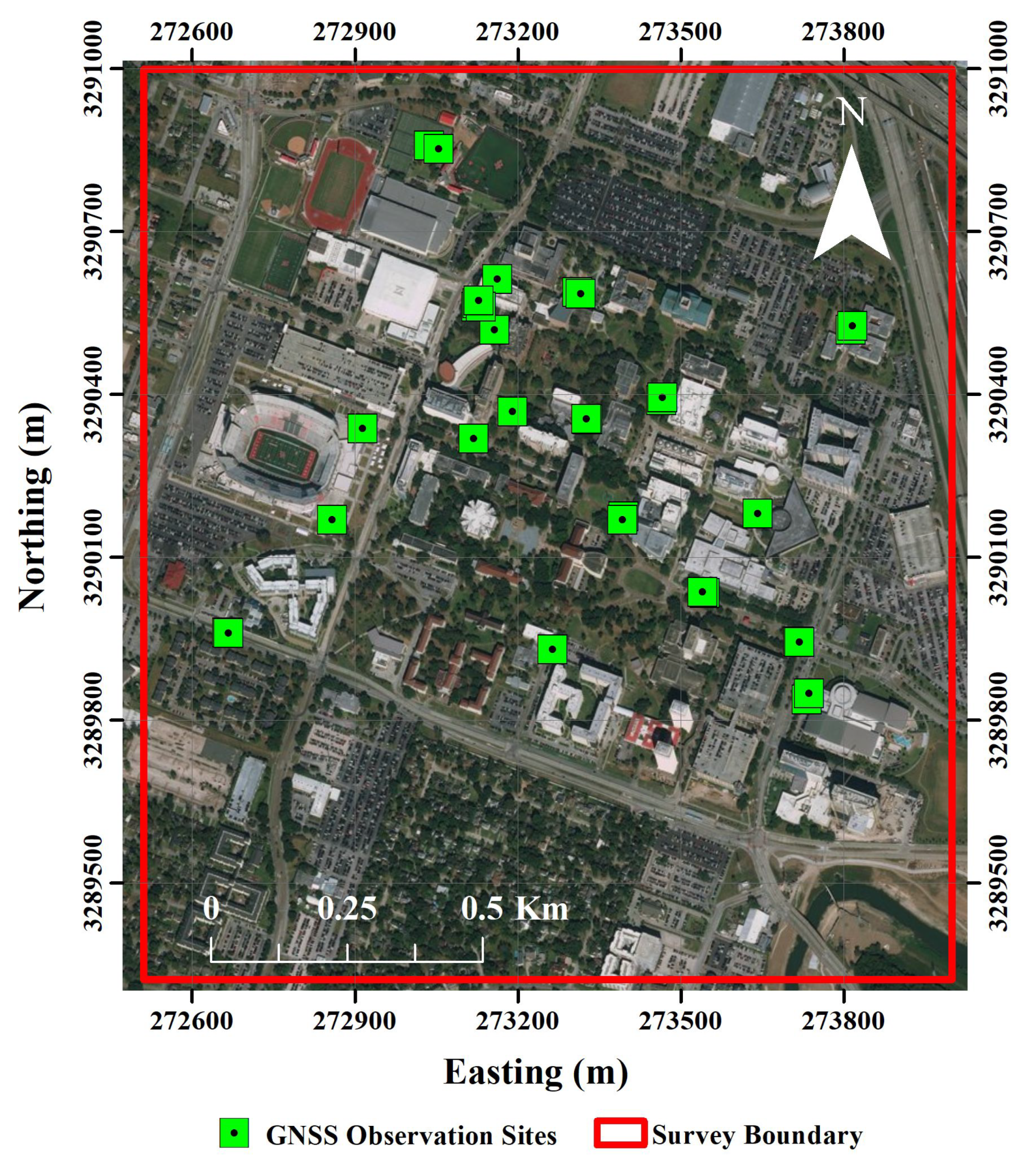
Global Navigation Satellite System (GNSS) data was collected throughout the University of Houston campus in November 2018. Because this survey was conducted long after the lidar collections, each site was carefully chosen to ensure it could be clearly distinguished in the SPL and LML point clouds and that its location had not changed. Candidate sites had flat surfaces and sharp, distinct corners (e.g., raised flower beds, benches, concrete blocks). In the field, a rapid static survey was performed at thirty-three different sites (Figure 1) using a Trimble NetR9 GNSS receiver, with each site observed for at least 40 min.
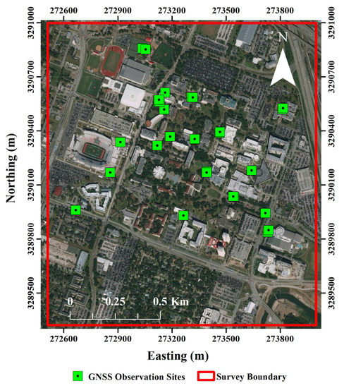
Figure 1.
University of Houston campus survey area and GNSS observation sites. Tick labels are Universal Transverse Mercator (UTM) Zone 15N.
The collected GNSS data was post-processed via the National Geodetic Survey’s (NGS) Online Positioning User Service (OPUS) website [15] and the software package GrafNet, which was used to manually post-process data on days where OPUS produced poor results. OPUS is a free web-based service that allows users to upload GNSS data and returns an email report containing the post-processed positional coordinates and quality information. OPUS has two different processing algorithms depending on the length of the data observation: OPUS-S for static data between 2 and 48 h, and OPUS-RS for rapid static data between 15 min and 2 h. OPUS-RS was used to process the data collected for this survey. Under normal conditions, OPUS-RS is capable of centimeter-level accuracy [16].
2.2. Methods
2.2.1. Positional Accuracy
The SPL100 data was transformed to the same horizontal and vertical datums as the Titan collection using the National Oceanic and Atmospheric Administration’s (NOAA) free software VDatum. The SPL horizontal UTM coordinates were shifted from WGS84(G1762) to NAD83(2011), and the elevations were transformed from WGS84(G1762) ellipsoid elevations to NAVD88 orthometric elevations (based on the NGS conterminous USA high-resolution geoid model Geoid12B). The areas of interest (the GPS collection sites) were then extracted from the full point clouds and displayed in MATLAB® to manually determine the closest point cloud position corresponding to each GPS site. The differences in the horizontal and vertical positions were recorded for every survey location for both the SPL and LML data sets.
2.2.2. Positional Precision
The precision of a lidar system can be inferred from measuring the dispersion of elevation values on flat surfaces within a single flight line. The Terrascan software package was used to identify and export fifty planar regions throughout the survey site; samples were saved as LAS files to preserve relevant metadata (intensity, flight line, GPS time stamp). These planar regions, which were at least 10 m2 in surface area, were chosen to include a variety of surface materials and slopes. Many of these samples came from rooftops of commercial and residential homes, but other flat regions such as sidewalks, tennis courts, and parking lots were also used. The same sample regions were used to analyze both the SPL and LML data sets.
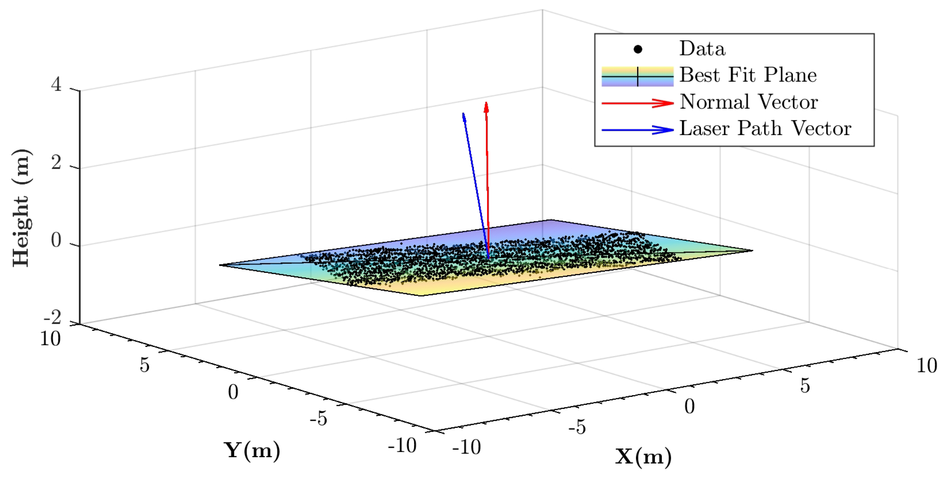
For each sample planar region, MATLAB® was used to determine the standard deviation of the lidar points with respect to a best fit plane (i.e., the measure of dispersion), the incidence angle at which the plane was observed, and the mean intensity of the returns from the plane. The best fit plane for each planar region is defined by the centroid of the points and the direction of a vector normal to the surface of a plane that intersects the centroid and minimizes the sum of the squared orthogonal distances between the points and the plane (i.e., the sum of the squared point-to-plane residuals). The centroid location is simply the mean of each of the point coordinate components. The normal vector and the standard deviation of the planar fit were computed from a singular value decomposition of the centroid-removed point coordinates. The smallest singular vector is normal to the best fit plane; the smallest singular value is the square root of the sum of the squared point-to-plane residuals, from which the standard deviation is easily computed [17]. A sample planar region of points, the best fit plane, and the normal vector to the best fit plane are illustrated in Figure 2.

Figure 2.
Illustration of a sample region of planar points (black dots), the planar surface best fit to the points, the vector normal to the best fit plane (red vector), and the laser path vector from the plane to the airborne sensor at the time of observation (blue vector). The incidence angle at which the plane was observed is computed as the angle between the normal and laser path vectors.
Computation of the incidence angle requires knowledge of the sensor location when the plane was observed. For each plane, the position of the first time-stamped point was used to construct a laser path vector, i.e, the vector from the planar patch to the airborne sensor at the time of observation. The incidence angle is the angle between this laser vector and the best fit plane normal vector, and is computed from the dot product of the vectors as , where and are the normal and laser vectors and the double bars indicate vector length. Note that only points from a single flight line were used, thus removing the possible effects of misalignments between flight lines as well as ambiguity regarding the sensor location.
2.2.3. DEM Comparison
Before a DEM can be generated, lidar returns from the ground must first be identified. This classification was performed using the TerraScan embedded ground classification routine, based on work by [18], with the default parameters (88 for terrain angle, 10 for iteration angle, and 1.4 m for iteration distance). Prior to analysis, the SPL data set was transformed to the same datum as the LML data, as described previously. Additionally, the mean elevation bias was subtracted from each data set, where the elevation bias is the mean value calculated from the differences between each GPS survey height and the height of the corresponding point cloud return.
The entire process of generating and comparing DEMs was done with Esri’s ArcMap software. A one-meter resolution image was created for both the LML and SPL data using the default parameters (cell assignment based on average value and void filling with linear interpolation). Each DEM raster image was then clipped to the same spatial extent in ArcMap to ensure matching boundaries before the LML image was subtracted from the SPL using Esri’s Raster Calculator tools.
2.2.4. Canopy Penetration and Multiple Returns
TerraScan was used to identify areas where the tree canopy completely covered the ground. Those trees were then segmented out and exported to LAS files that could be further analyzed and plotted in MATLAB®. An important part of this analysis was determining how many of the emitted pulses reached the ground. To accomplish this, the cloth simulation filtering (CSF) algorithm [19] was used to classify ground points. The CSF algorithm creates a surface model by inverting the point cloud and simulating a cloth draped over the terrain. It has been made available in a variety of programming languages, including Python and MATLAB®, as well as a plugin for the open-source program CloudCompare. The CSF algorithm was more effective at creating a suitable classification for these small sample areas than using TerraScan. The following CSF parameters were used: 0.1 for cloth resolution, 500 iterations maximum, and 0.1 classification threshold. Multiple returns were identified by a return number greater than 1 in the LAS point records and grouped according to time (multiple returns originate from the same emitted laser pulse and thus are stamped with the same time).
3. Results and Discussion
3.1. Positional Accuracy
Accuracy was assessed by examining the mean horizontal and vertical differences between the 33 GNSS collection sites and their corresponding LML and SPL point cloud positions (see Table 2 and Table 3). Using the standard deviations of the horizontal and vertical differences, Z-tests were performed to determine if the mean differences in easting, northing, and height were statistically different from zero at a 95% confidence level. With one exception (the mean northing difference of the Titan data), the horizontal differences are statistically equal to zero, but the vertical differences are not. Those components with differences not statistically equal to zero indicate a systematic bias in the point clouds, potentially from the kinematic trajectory solution or strip adjustments applied during point cloud processing.

Table 2.
Optech Titan horizontal and vertical differences from GNSS points.

Table 3.
Leica SPL100 horizontal and vertical differences from GNSS points.
The presence of vertical biases in both the LML and SPL data aligns with the knowledge that the vertical component of GNSS positions and, hence, trajectory solutions is weaker than the horizontal components. Noting that the SPL100 data has a positive elevation bias (11.67 cm) and the Titan has a negative elevation bias (−13.27 cm), and that these differences are statistically different from zero at 95% confidence, it is clear that the elevation difference between the SPL100 and Titan data is statistically significant. However, if the vertical biases are examined in terms of their magnitude only, there is no statistical difference at 95% confidence according to a two-sample Z-test. This indicates that the vertical accuracies of the LML and SPL data are similar.
Overall, these results indicate the LML and SPL data are of similar positional accuracy (closeness to truth, as determined by GNSS ground observations) in regards to the final post-processed data product. Indeed, the SPL data outperforms the LML data in this small test area since only the vertical component was found to be statistically different from zero, whereas both the northing and vertical components of the LML data were statistically different from zero.
It is noted that the large standard deviations for the horizontal components in Table 2 and Table 3 stem from the lack of lidar points at the exact locations of the features occupied with GNSS. As expected, the horizontal standard deviation magnitudes are inversely proportional to the nominal point densities of the two point clouds (SPL100 ≈ 25 points/m, Titan ≈ 12 points/m). Given the sample size (33 GNSS sites) and the assumption of randomness in the direction between each GNSS feature location and the closest lidar point, the impact on the accuracy assessment is mitigated since the random errors should largely cancel out in the mean difference computations reported in Table 2 and Table 3. Note, however, that the large standard deviations appropriately influence our interpretation of whether the mean differences between the GNSS and closest lidar point locations are significant. For example, the mean easting difference between the GNSS and SPL100 data is almost −3 cm. Although this is clearly different from zero, it is intuitively insignificant (backed up by the Z-statistic test) in the presence of the relatively large standard deviation of ±11 cm.
A recent publication by Kim et al. [20] proposes a method based on terrestrial laser scanning rather than single GNSS point locations to avoid the influence of point density on airborne lidar data accuracy evaluations. This is accomplished by modeling and intersecting multiple planar surfaces on residential rooftops, using data from both terrestrial (which serves as the reference data of higher accuracy) and airborne lidar point clouds, to produce synthetic conjugate points for comparison. However, our test area (the University of Houston campus) is dominated by tall buildings with flat roofs, which are not easily collected with terrestrial laser scans. It is also noted that the data collection and processing requirements of the proposed method are significantly more (perhaps an order of magnitude) than that required for the method applied in this work.
3.2. Positional Precision
The planar standard deviations of flat regions—used as a measure of positional precision, i.e., measurement consistency—were higher in the SPL100 data set than in the Titan linear mode lidar data. The overall standard deviation, calculated from all residuals across the 50 chosen planar samples, was 3.2 cm for the SPL100. In the Titan data, however, it was less than half of that, approximately 1.2 cm. When standard deviations were calculated for each sample, the SPL100 also had a much broader range of standard deviations from 1 cm up to 11 cm. The sample standard deviations for the Titan ranged from a minimum of 0.5 cm to approximately 3 cm. A two-sample F-test was conducted for each sample to determine whether the differences in planar variances in the SPL and LML data were statistically significant at 95%. Of the 50 samples, only three of the variances were found not to be statistically different.
The lower positional precision for the SPL100 compared to the LML system is an expected result for a few reasons. First, the SPL100 data was acquired from an AGL seven times higher than the Titan data, thus magnifying the impact of angular noise in the trajectory solution on the georeferenced lidar point coordinates. Second, SPL ranges inherently suffer from a greater amount of random error than LML ranges. In a LML detector, hundreds to thousands of photons are returned to the detector, allowing a temporal profile of the return power to be formed that can be modeled for a precise peak location. In the case of single photon detectors, only a few photons are returned and only a single photon is detected. The temporal power profile can not be modeled and there is uncertainty as to where in the temporal power profile the single detected photon exists. Although this explanation is greatly simplified, it provides a sense of the source of the greater uncertainty, or noise, in SPL ranges compared to LML ranges.
To better understand how other variables may be affecting the observed planar standard deviations, mean intensity and incidence angle were examined with respect to the planar fit standard deviations. Lidar range finder precision has been shown to decrease with low intensity [21] because the precision of range estimation is proportional to the signal-to-noise ratio (SNR) [22]. In LML systems, intensity values are a measure of the strength of the returning laser pulse, and typically the peak amplitude is used. For single photon sensitive systems, intensity is not a native product since only one photon is detected. However, the SPL100 reports an intensity for each detected return. This capability stems from the use of a detector (silicon photomultiplier) that can register multiple single photon detection events in each detector channel and sum the output to form an intensity measure; see [23] for an examination of the intensity values reported by the SPL100.
Graphs of intensity versus planar standard deviation for both the SPL100 and the Titan data are given in Figure 3. For both sensors, decreasing precision corresponds to decreasing intensity. A recent study by [21] found that in laboratory-controlled conditions with calibration targets, the range error in a terrestrial lidar system decreased non-linearly as the recorded intensity increased. A power function was used to model the non-linear relationship between ranging precision (standard deviation of recorded ranges) and intensity. Assuming that the behavior of real-world targets will bear some resemblance to those under laboratory-controlled conditions, the following equation was used to model planar standard deviation () as a function of lidar intensity (I), where a, b, and c are unknown parameters:
A best fit curve of the form of Equation (1) is overlaid on the data points in Figure 3. Although the power law equation does not appear to be unreasonable, systematic differences at high and low intensities are seen between the SPL100 data points and best fit curve, whereas the LML data points are quite noisy and preclude any definitive statements. However, qualitative inspection suggests the power law equation may be more appropriate for the LML data than the SPL data.

Figure 3.
Variation of planar standard deviation with mean intensity for the (A) SPL100 and (B) Titan 532 nm channel. A least squares fit of a power function in the form of Equation (1) is shown for both.
In addition to mean intensity, the effect of incidence angle on the observed planar standard deviations was also considered. Graphs for incidence angle versus the standard deviation of planar residuals for both the SPL100 and the Titan data are given in Figure 4. Both the SPL100 and the Titan sensor show an increase in standard deviation with increased incidence angle. However, the increase, as measured by the slope of a best fit line, is an order of magnitude steeper for the SPL100 compared to the Titan data. The linear trend of standard deviation is in approximate agreement with [22]’s well-known characterization of maximum ranging error as a function of incidence angle:
where is incidence angle, h is flying height above ground, and is laser beam divergence. For angles less than 60, which is the maximum shown in Figure 4, Equation (2) is approximately linear. However, the errors predicted by Equation (2) are much larger than observed in Figure 4. For example, at 40 incidence, Equation (2) predicts ranging errors of 0.12 m for the SPL100 (twice as large than observed) and 0.21 m for the Titan (order of magnitude larger than observed). Note that mrad for each SPL100 beamlet and mrad for the Titan 532 channel. Empirical modeling of ranging error as a function of return intensity or incidence angle may therefore be more appropriate than Equation (2) for applications such as lidar total propagated uncertainty estimation (e.g., see [24,25]).

Figure 4.
Variation of planar standard deviation with planar incidence angle for the (A) SPL100 and (B) Titan 532 nm channel. Best fit line shown. The data points are colored by the mean intensity of each planar surface.
The effects of intensity and incidence angle are correlated, as a high incidence angle causes a reduction in return intensity for smooth surfaces. Thus, a high noise level could be explained by either a bright surface recorded at a high incidence angle or a dark surface observed at a low incidence angle [21]. This correlation is seen in Figure 4, where the data points are colored by intensity values and the higher incidence points are dominantly lower intensity returns.
3.3. DEM Comparison
In Figure 5, two one-meter resolution maps show the difference between DEMs derived from the Titan and two SPL100 DEMs generated from data processed with two different versions of HxMap. There are artifacts in and around buildings in both difference images due to occlusions and misclassifications from the ground filtering routines. Water bodies such as the bayou (southeast corner) and man-made ponds also differ in elevation between the SPL100 and Titan data because the ground classification routine did not identify the Titan bathymetry as ground returns, while the SPL100 bathymetry was identified as ground.
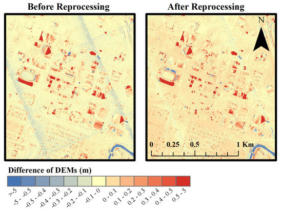
Figure 5.
Difference of DEMs (SPL100–Titan) using HxMap software in 2017 (left side) and after using updated HxMap software in 2019 (right side).
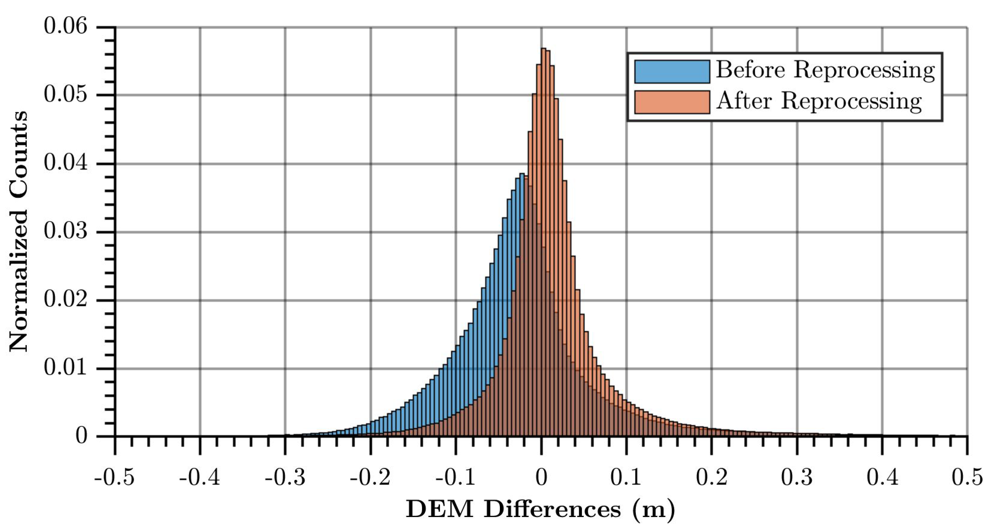
More significantly, the SPL100 point cloud generated by the HxMap software in 2017 (when the lidar data was collected) contains noticeable artifacts at the edges of the SPL100 flight lines, visible as a large, tilted square approximately centered in the DEM difference image. At these edges, the SPL100 DEM differs from the Titan DEM by about 4 cm. Reprocessing the raw data in 2019 revealed that recent updates to the HxMap software have improved the post-processed data quality. In the right side of Figure 5, with a 2019 version of HxMap, the flight line artifacts have been improved, and the DEM is in closer agreement to the Titan derived DEM. These visual observations are confirmed with a histogram of the DEM differences (Figure 6), which shows a mean bias of −2.5 cm between the Titan DEM and the 2017 HxMap post-processed SPL100 data, and 1.4 cm using a more recent version (processed in 2019) of the HxMap software. Note that before the comparisons, the mean biases for each data set, as determined by the mean vertical difference from the GNSS survey locations (see Table 2 and Table 3), were first removed.
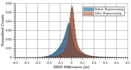
Figure 6.
Histogram of the DEM differences (SPL100–Titan) before and after reprocessing with a more recent version of HxMap.
Given that the SPL100 is marketed for large area terrain mapping, it should be capable of producing DEMs that are of comparable quality and accuracy to those currently produced from traditional LML systems. The close agreement between the SPL100 DEM generated from lidar data processed with the most recent version of HxMap and the Titan DEM suggests that the SPL100 largely meets these requirements, but small systematic problems still exist at the SPL100 flight line edges.
3.4. Canopy Penetration and Multiple Returns
The final analysis examined the ability of the SPL100 and Titan systems to penetrate the canopy, record multiple returns, and resolve closely spaced targets, the latter of which is referred to as range resolution. Note that the term multiple returns refers to the ability of a lidar sensor to record more than one return energy event, each of which produces a point in the eventual point cloud, for a single emitted laser pulse. For each emitted laser pulse, the returns are numbered by the order in which they are received by the lidar sensor. Statistics describing these characteristics, generated from thirty sample canopy areas, are shown in Table 4. It can be readily observed that even though the SPL100 produces more laser returns than the Titan, the Titan generates more multiple and ground returns as a percentage of the total pulses emitted.

Table 4.
Canopy penetration and multiple return statistics.
Of the thirty sampled tree canopies, only 22% of SPL100 emitted pulses had multiple returns, as compared to 87% for the Titan. The SPL100 usually generated only one or two returns through the canopy. Although a small number of pulses had three returns, they made up less than 1% of the total pulses analyzed. In contrast, pulses with three or four returns comprised 50% of the total emitted pulses in the Titan samples.
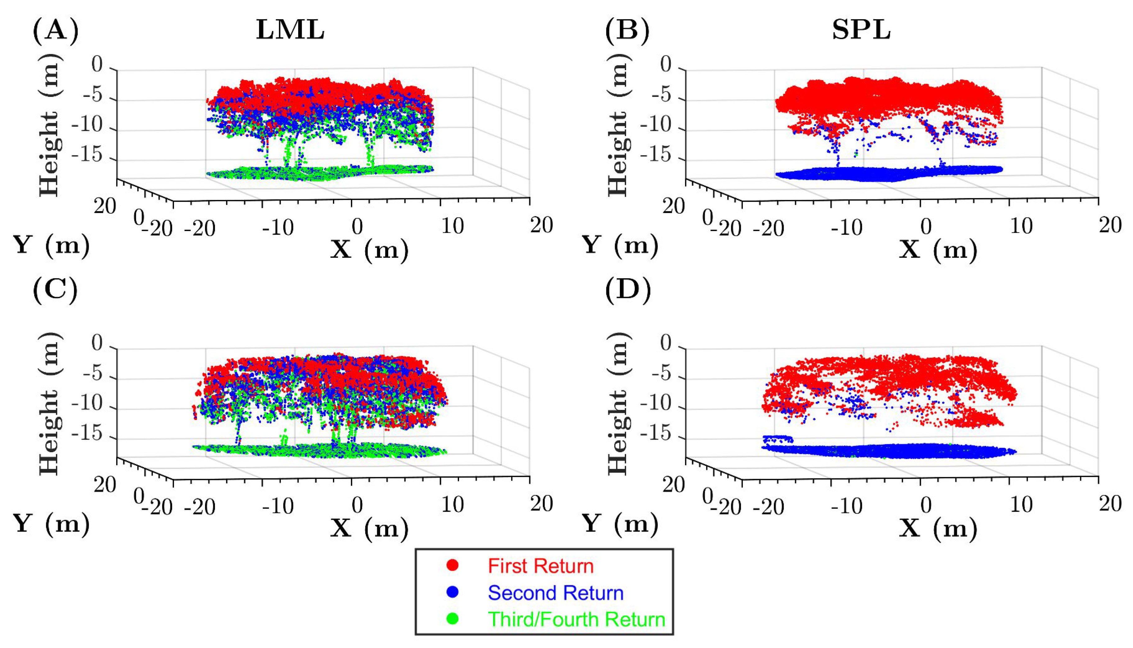
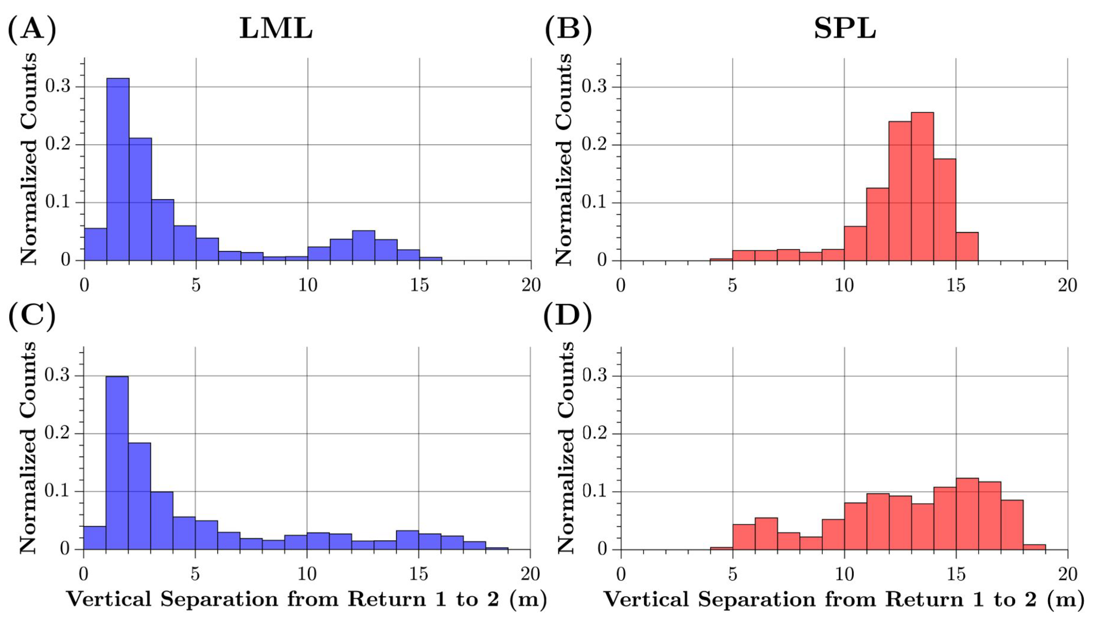
It is apparent that, in terms of range resolution, the SPL100 is considerably more limited than an LML system. On average, the first and second returns had about 10 m of vertical separation, and only a small fraction of the second returns came from lower in the canopy. Visual inspection of the point cloud, colored by return number, and the histogram of range separations shows that the second returns in the SPL100 are overwhelmingly from the ground (Figure 7 and Figure 8). The first and second returns in the Titan are separated, on average, by 4.3 m. This average, however, comes from a bimodal distribution made of up second returns from the canopy and on the ground. Although they did not directly look at vertical separation, [10] also reported that the SPL100 had significantly less average returns per pulse: 1.06 returns through thick vegetation, as compared to 1.84 mean returns using a full-waveform lidar system.
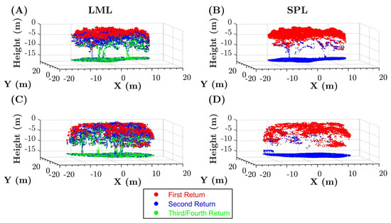
Figure 7.
Tree canopy examples colored by return number (the lidar sensors have the ability to detect and record more than one return energy event for each emitted laser pulse). First returns are red, second returns are blue, third and fourth returns are green. Titan data is shown in the left column (panels (A) and (C)) and SPL100 data in the right column (panels (B) and (D)).
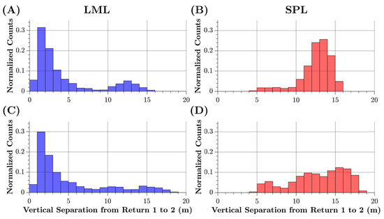
Figure 8.
Histograms of range distance between first and second returns for the tree canopy examples shown in Figure 7. Titan data is shown in the left column (panels (A) and (C)) and SPL100 data in the right column (panels (B) and (D)).
Previous studies using the SPL100’s predecessor, the HRQLS, specify that the system has a 1.6 ns pixel recovery time, and is thus capable of recording returns separated by 24 cm [1,2]. However, the observed SPL100 range resolution is not due to the detector characteristics, but rather due to noise filtering. During post-processing, a dead distance filter is applied to the SPL100 data to eliminate after-pulsing noise (personal communication with Zhigang Pan, Leica Geosystems [26]). However, this filter also removes a significant amount of multiple returns in vegetation, which are important for canopy penetration. The range resolution of unfiltered SPL100 data was therefore analyzed to validate this assumption. Unfiltered SPL data has a large column of noise extending above and below the surface returns. To get around this limitation, any noise points above the canopy or below the ground level were removed. The return numbers of the remaining points were then adjusted so that first returns could only occur within the bounding box.
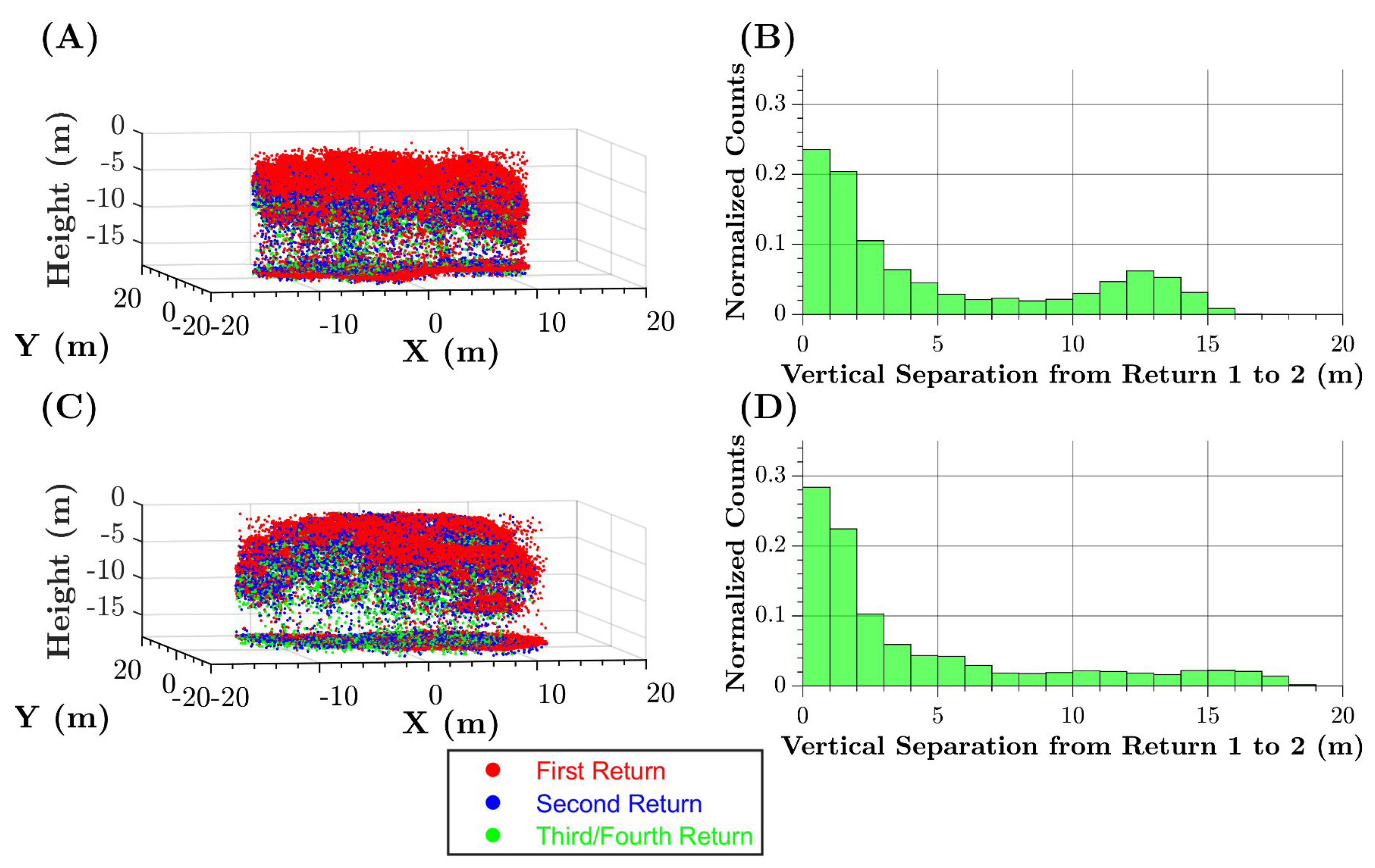
As depicted in Figure 9, the unfiltered SPL100 has multiple returns distributed throughout the canopy. On average, the first and second returns in the unfiltered SPL100 point cloud are separated by 4.0 m, which is slightly better than what was observed with the Titan data. This average, of course, does account for the inclusion of noise returns. These results confirm that SPL100 range resolution is presently limited by noise filtering. In the future, it may be possible to address this issue with more sophisticated noise filtering algorithms.
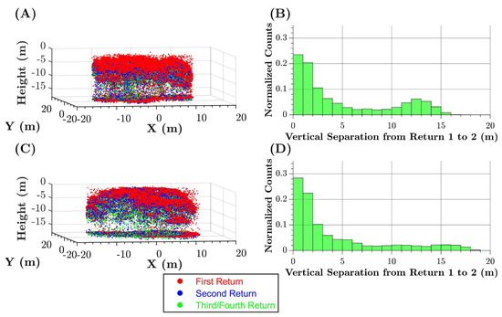
Figure 9.
Tree canopy examples colored by return number for the unfiltered SPL100 point clouds (left column, panels (A) and (C)). First return is red, second return is blue, third and fourth returns are green. Histograms of range distance between first and second returns (right column, panels (B) and (D)). The canopy examples are the same as in Figure 7.
In addition to producing more pulses with multiple returns, more of the pulses reached the ground with the Titan (71%) than in the post-processed SPL100 (44%). However, for the samples tested here, the Titan data had a point density of about 10 points/m2 under the treetops while the SPL100 data had about 28 points/m2. The reason the SPL100 is capable of generating higher ground densities under tree canopies, as compared to the Titan, is due to the higher number of lidar measurements (i.e., emitted pulses) rather than superior penetration performance. This is reinforced by the work in [10], where SPL100 and LML data acquisitions were planned to achieve similar overall point density (20 points/m2), and the LML point density under vegetation surpassed that of the SPL100. In general, an LML sensor with an equivalent ground sampling rate as the SPL100 will surpass the SPL100 in under-canopy point density.
Lastly, this analysis considered the ranging precision of flat terrain under the treetops as compared to adjacent areas of open terrain with roughly the same land cover. Under canopy cover, flat terrain had an overall standard deviation of 3.6 cm (computed from all residuals for 25 samples) and 3.0 cm in open terrain (Table 5) for the SPL100. In contrast, the Titan precision improved from a standard deviation of 2.7 cm under the canopy to nearly half that, 1.7 cm, in open terrain. A two-sample F-test determined that for both systems, differences in planar variances were statistically significant at 95% when comparing the residuals of samples under the canopy and those in open terrain.

Table 5.
Planar surface dispersion under canopy and in open terrain.
These results are roughly in line with [10], although they did not look into standard deviation statistics under the canopy. They found that the SPL100 had a dispersion of about 3.9 cm in open meadows while in a full-waveform LML system, it was 1.0 cm. In their examination of the HRQLS’s ability to meet the needs of the USGS, [2] raised concerns that the vertical accuracy in vegetated areas for the bare-earth DEMs was unacceptable during leaf-on conditions. The reduced accuracy was attributed to noisier points and larger voids under the canopy as compared to LML. The results presented here, however, are not directly comparable due to differences in study sites. The study from [2] considered both a forested region in addition to an urban area, while this analysis looked mainly at small groves of trees in urban areas, typically with manicured lawns underneath. Only a few areas of denser tree cover, such as parks and empty lots, were included. Further research is needed to test whether the SPL100 is capable of acceptable accuracy under dense canopy for non-urban areas.
4. Conclusions
Point cloud precision and accuracy, DEM quality, and canopy penetration performance of the Leica SPL100 were examined in this work. The results align with the expectation of lower ranging precision for the SPL100 than for LML systems, and also demonstrate that the SPL100 precision is more negatively affected by surface properties of radiometric brightness and incidence angle compared to a LML system. For the fifty planar surfaces tested, the SPL100 showed a much larger range of standard deviations, from 1 up to 11 cm. The LML data, collected with an Optech Titan, had planar standard deviations that only ranged from 0.5 to 3 cm. Taking the residuals of all the samples together, the SPL100 had an overall standard deviation of 3.2 cm, while the Titan had an overall standard deviation of 1.2 cm. However, even though the SPL100 was flown from a significantly higher flying height and has worse ranging precision, comparison to GNSS survey data indicated the post-processed SPL100 point cloud has similar positional accuracy to that of the LML data, at least for the urban area tested. Furthermore, the DEM derived from the SPL100 closely agrees with the DEM produced from the Titan data, with a small mean difference of 1.4 cm. Recent updates to Leica’s HxMap also show improved post-processed data quality, with biases at the SPL100 flight line edges greatly reduced.
Only one or two returns are to be expected in vegetation from the post-processed SPL100 data. In the samples tested, the first and second returns had, on average, a vertical separation of about 10 m. Most of the second returns came from the ground, rather than lower in the canopy. In contrast, the Titan data contains multiple returns that were well distributed throughout the canopy, with first and second returns separated by 4.3 m, on average. Analysis of unfiltered SPL100 data confirmed that noise filtering applied during post-processing was the primary reason for the relatively poor range resolution in the SPL100, as the algorithm removes a portion of the multiple returns. The unfiltered data set had a similar ability to resolve multiple returns as the LML, with an average of 4.0 m between the first and second returns within the canopy. In the future, more sophisticated noise-filtering algorithms may be able to better preserve valid returns while removing spurious noise points. Planar standard deviations under canopy (3.6 cm) were only slightly higher than in open terrain (3.0) for the SPL100. This indicates the primary challenge for the SPL100 in achieving high quality surfaces under tree canopy is in generating sufficient point density to accurately model the terrain morphology.
In its current state, the SPL100 is likely best suited for applications in which the need for data collection efficiency outweighs the need for the best possible accuracy and precision. Despite its lower ranging precision, the SPL100 is nonetheless capable of accuracy similar to LML for flat, open terrain. Going forward, single photon lidar and Geiger-mode lidar systems will benefit from additional research so that users of these new technologies will have a thorough understanding of best practices for data collection and processing. In particular, future studies should focus on the SPL100’s positional accuracy on sloped and textured surfaces, including terrain under vegetation cover. It has been demonstrated in this work and elsewhere that such conditions significantly worsen ranging precision, but more information is needed to quantify its effect on accuracy. The SPL100’s suitability for forestry applications should also be examined in light of the knowledge that noise filtering removes returns in the canopy.
Author Contributions
Conceptualization, C.G.; Methodology, C.G., P.H., R.B.; Investigation, R.B.; Writing–original draft preparation, R.B.; Writing–review and editing, P.H., C.G.; Supervision, P.H., C.G.; Project Administration, R.B.; Funding Acquisition, C.G. All authors have read and agreed to the published version of the manuscript.
Funding
This research was partially supported by grants from the National Science Foundation Instrumentation and Facilities program (#1830734) and the U.S. Army Engineer Research and Development Center Cold Regions Research and Engineering Laboratory Remote Sensing/GIS Center of Expertise.
Acknowledgments
The authors would like to thank Leica Geosystems for providing access to the SPL100 data. Darren Hauser, Abhinav Singhania and Juan-Carlos Fernandez-Diaz of the National Center for Airborne Laser Mapping are also thanked for assisting with the Titan data.
Conflicts of Interest
The authors declare no conflict of interest.
References
- Degnan, J.J. Scanning, Multibeam, Single Photon Lidars for Rapid, Large Scale, High Resolution, Topographic and Bathymetric Mapping. Remote Sens. 2016, 8, 958. [Google Scholar] [CrossRef]
- Stoker, J.M.; Abdullah, Q.A.; Nayegandhi, A.; Winehouse, J. Evaluation of Single Photon and Geiger Mode Lidar for the 3D Elevation Program. Remote Sens. 2016, 8, 767. [Google Scholar] [CrossRef]
- Swatantran, A.; Tang, H.; Barrett, T.; DeCola, P.; Dubayah, R. Rapid, High-Resolution Forest Structure and Terrain Mapping over Large Areas using Single Photon Lidar. Sci. Rep. 2016, 6, 28277. [Google Scholar] [CrossRef] [PubMed]
- Degnan, J.; Machan, R.; Leventhal, E.; Lawrence, D.; Jodor, G.; Field, C. Inflight performance of a second-generation photon-counting 3D imaging lidar. In Laser Radar Technology and Applications XIII; Turner, M.D., Kamerman, G.W., Eds.; International Society for Optics and Photonics, SPIE: Bellingham, WA, USA, 2008; Volume 6950, pp. 32–40. [Google Scholar] [CrossRef]
- Ullrich, A.; Pfennigbauer, M. Linear LIDAR versus Geiger-mode LIDAR: Impact on data properties and data quality. In Laser Radar Technology and Applications XXI; Turner, M.D., Kamerman, G.W., Eds.; International Society for Optics and Photonics, SPIE: Bellingham, WA, USA, 2016; Volume 9832, pp. 29–45. [Google Scholar] [CrossRef]
- Ullrich, A.; Pfennigbauer, M. Noisy lidar point clouds: Impact on information extraction in high-precision lidar surveying. In Laser Radar Technology and Applications XXIII; Turner, M.D., Kamerman, G.W., Eds.; International Society for Optics and Photonics, SPIE: Bellingham, WA, USA, 2018; Volume 10636, pp. 133–138. [Google Scholar] [CrossRef]
- Jutzi, B. Less Photons for more LiDAR? A Review from Multi-Photon-Detection to Single-Photon-Detection. In Proceedings of the 56th Photogrammetric Week (PhoWo 2017), Stuttgart, Germany, 11–15 September 2017; p. 6 S. [Google Scholar]
- Degnan, J.J.; Field, C.T. Moderate to high altitude, single photon sensitive, 3D imaging lidars. In Advanced Photon Counting Techniques VIII; Itzler, M.A., Campbell, J.C., Eds.; International Society for Optics and Photonics, SPIE: Bellingham, WA, USA, 2014; Volume 9114, pp. 56–66. [Google Scholar] [CrossRef]
- Heidemann, H.K. Lidar Base Specification; Technical report; U.S. Geological Survey: Reston, VA, USA, 2012. [CrossRef]
- Mandlburger, G.; Lehner, H.; Pfeifer, N. A Comparison of Single Photon and Full Waveform Lidar. ISPRS Ann. Photogramm. Remote Sens. Spat. Inf. Sci. 2019, IV-2/W5, 397–404. [Google Scholar] [CrossRef]
- Wästlund, A.; Holmgren, J.; Lindberg, E.; Olsson, H. Forest Variable Estimation Using a High Altitude Single Photon Lidar System. Remote Sens. 2018, 10, 1422. [Google Scholar] [CrossRef]
- Fernandez-Diaz, J.C.; Carter, W.E.; Glennie, C.; Shrestha, R.L.; Pan, Z.; Ekhtari, N.; Singhania, A.; Hauser, D.; Sartori, M. Capability Assessment and Performance Metrics for the Titan Multispectral Mapping Lidar. Remote Sens. 2016, 8, 936. [Google Scholar] [CrossRef]
- Leica SPL100 Single Photon LidAR Sensor. Available online: https://leica-geosystems.com/en-us/products/airborne-systems/topographic-lidar-sensors/leica-spl100 (accessed on 12 January 2020).
- Titan. Available online: https://www.teledyneoptech.com/en/products/airborne-survey/titan/ (accessed on 12 January 2020).
- Mader, G.L.; Weston, N.D.; Morisson, M.L.; Milbert, D.G. The On-Line Positioning User Service (OPUS). Prof. Surv. 2003, 23, 26–30. [Google Scholar]
- Soler, T. CORS and OPUS for Engineers: Tools for Surveying and Mapping Applications; American Society of Civil Engineers: Reston, VA, USA, 2011. [Google Scholar]
- Shakarji, C. Least-squares fitting algorithms of the NIST algorithm testing system. J. Res. Natl. Inst. Stand. Technol. 1998, 103, 633. [Google Scholar] [CrossRef] [PubMed]
- Axelsson, P. DEM Generation from Laser Scanner Data Using Adaptive TIN Models. Int. Arch. Photogramm. Remote Sens. 2000, XXXIII, 110–117. [Google Scholar]
- Zhang, W.; Qi, J.; Wan, P.; Wang, H.; Xie, D.; Wang, X.; Yan, G. An Easy-to-Use Airborne LiDAR Data Filtering Method Based on Cloth Simulation. Remote Sens. 2016, 8, 501. [Google Scholar] [CrossRef]
- Kim, M.; Park, S.; Danielson, J.; Irwin, J.; Stensaas, G.; Stoker, J.; Nimetz, J. General external uncertainty models of three-plane intersection point for 3D absolute accuracy assessment of lidar point cloud. Remote Sens. 2019, 11, 2737. [Google Scholar] [CrossRef]
- Wujanz, D.; Burger, M.; Mettenleiter, M.; Neitzel, F. An intensity-based stochastic model for terrestrial laser scanners. ISPRS J. Photogramm. Remote Sens. 2017, 125, 146–155. [Google Scholar] [CrossRef]
- Baltsavias, E. Airborne laser scanning: Basic relations and formulas. ISPRS J. Photogramm. Remote Sens. 1999, 54, 199–214. [Google Scholar] [CrossRef]
- Hartzell, P.; Dang, Z.; Pan, Z.; Glennie, C. Radiometric Evaluation of an Airborne Single Photon Lidar Sensor. IEEE Geosci. Remote Sens. Lett. 2018, 15, 1466–1470. [Google Scholar] [CrossRef]
- Hartzell, P.J.; Gadomski, P.J.; Glennie, C.L.; Finnegan, D.C.; Deems, J.S. Rigorous error propagation for terrestrial laser scanning with application to snow volume uncertainty. J. Glaciol. 2015, 61, 1147–1158. [Google Scholar] [CrossRef]
- O’Banion, M.S.; Olsen, M.J.; Parrish, C.E.; Bailey, M. Interactive Visualization of 3D Coordinate Uncertainties in Terrestrial Laser-Scanning Point Clouds Using OpenGL Shader Language. J. Surv. Eng. 2019, 145, 04018012. [Google Scholar] [CrossRef]
- Pan, Z. Personal communication, 2019.
© 2020 by the authors. Licensee MDPI, Basel, Switzerland. This article is an open access article distributed under the terms and conditions of the Creative Commons Attribution (CC BY) license (http://creativecommons.org/licenses/by/4.0/).

