Quantifying Flood Water Levels Using Image-Based Volunteered Geographic Information


Abstract
1. Introduction
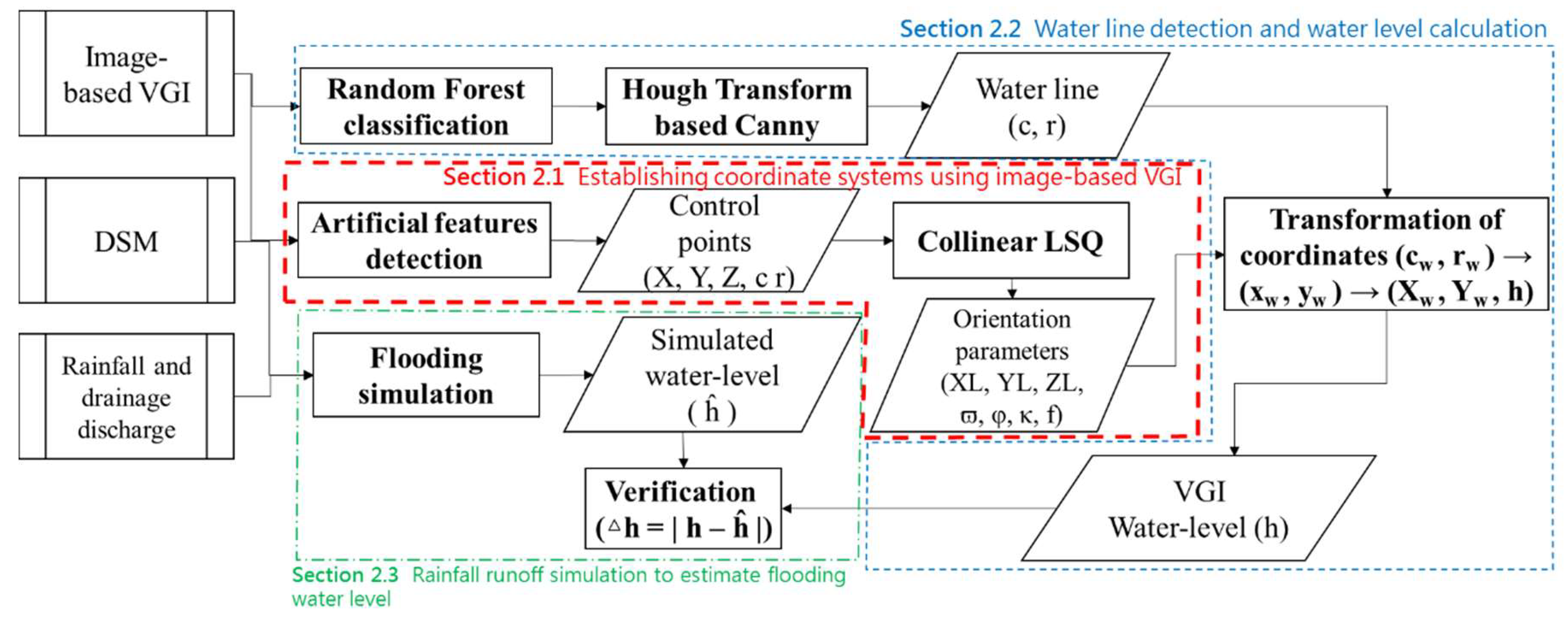
2. Methods
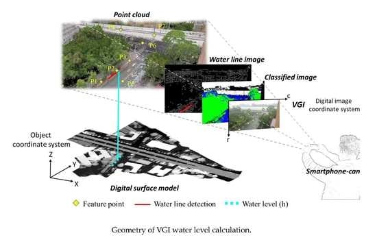
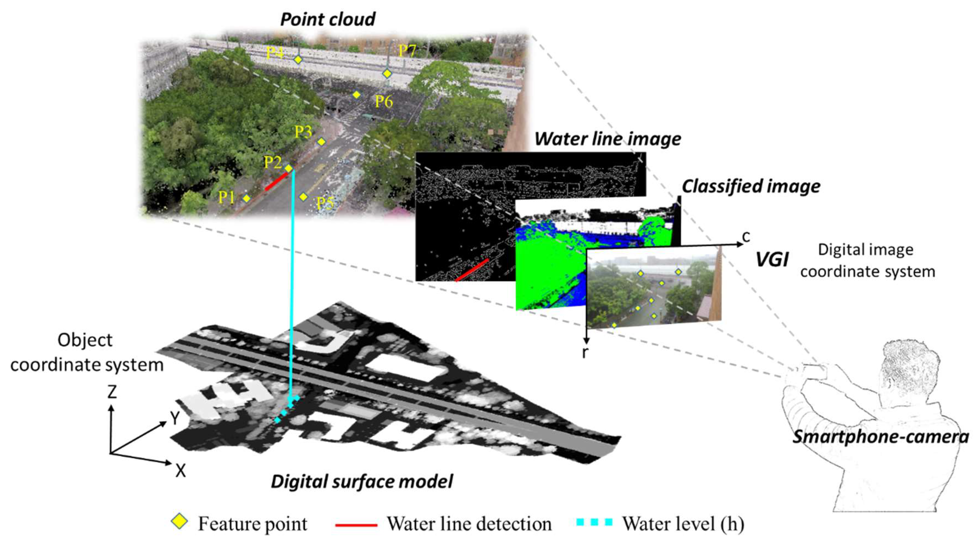
2.1. Establishing Coordinate Systems Using Image-Based VGI
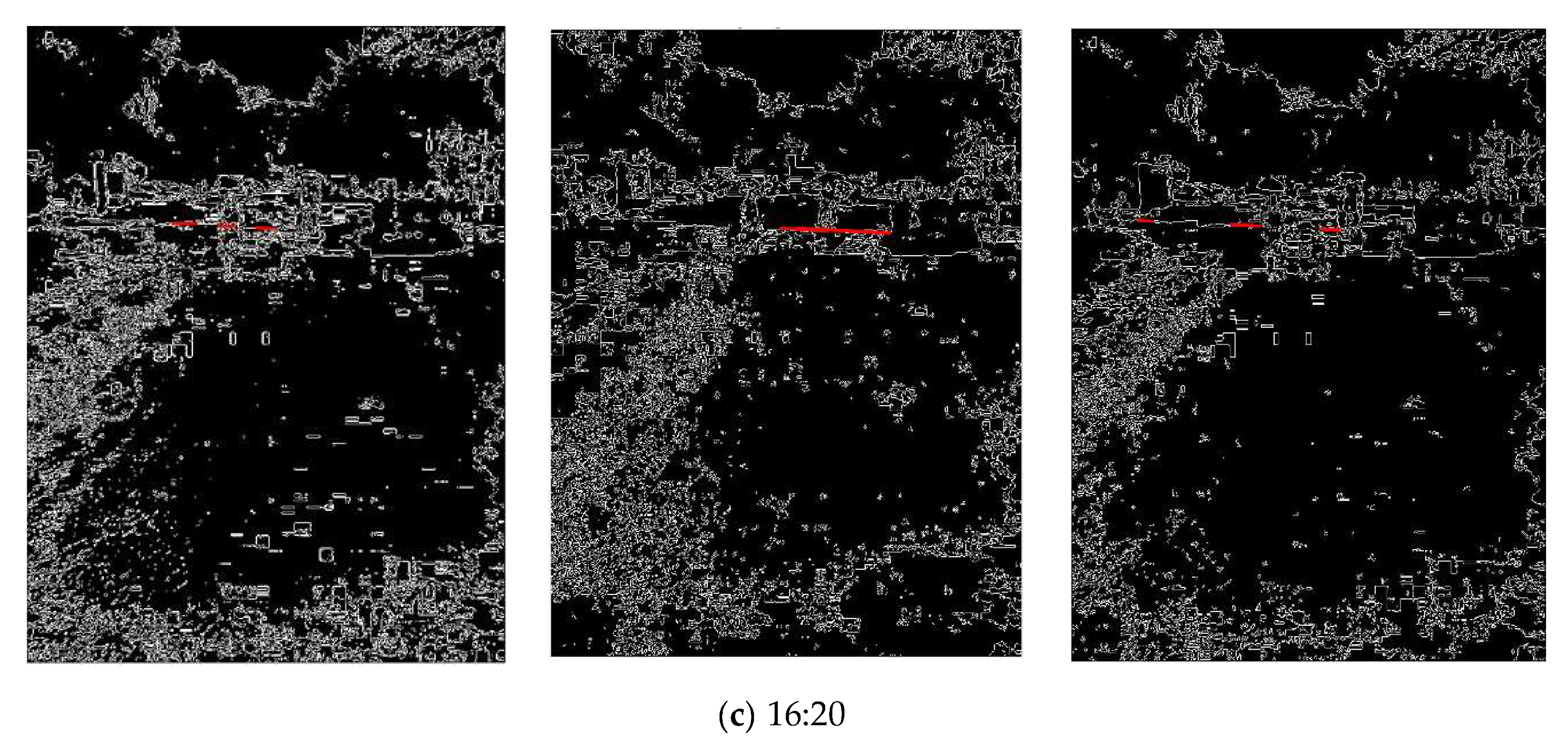
2.2. Water Line Detection and Water Level Calculation
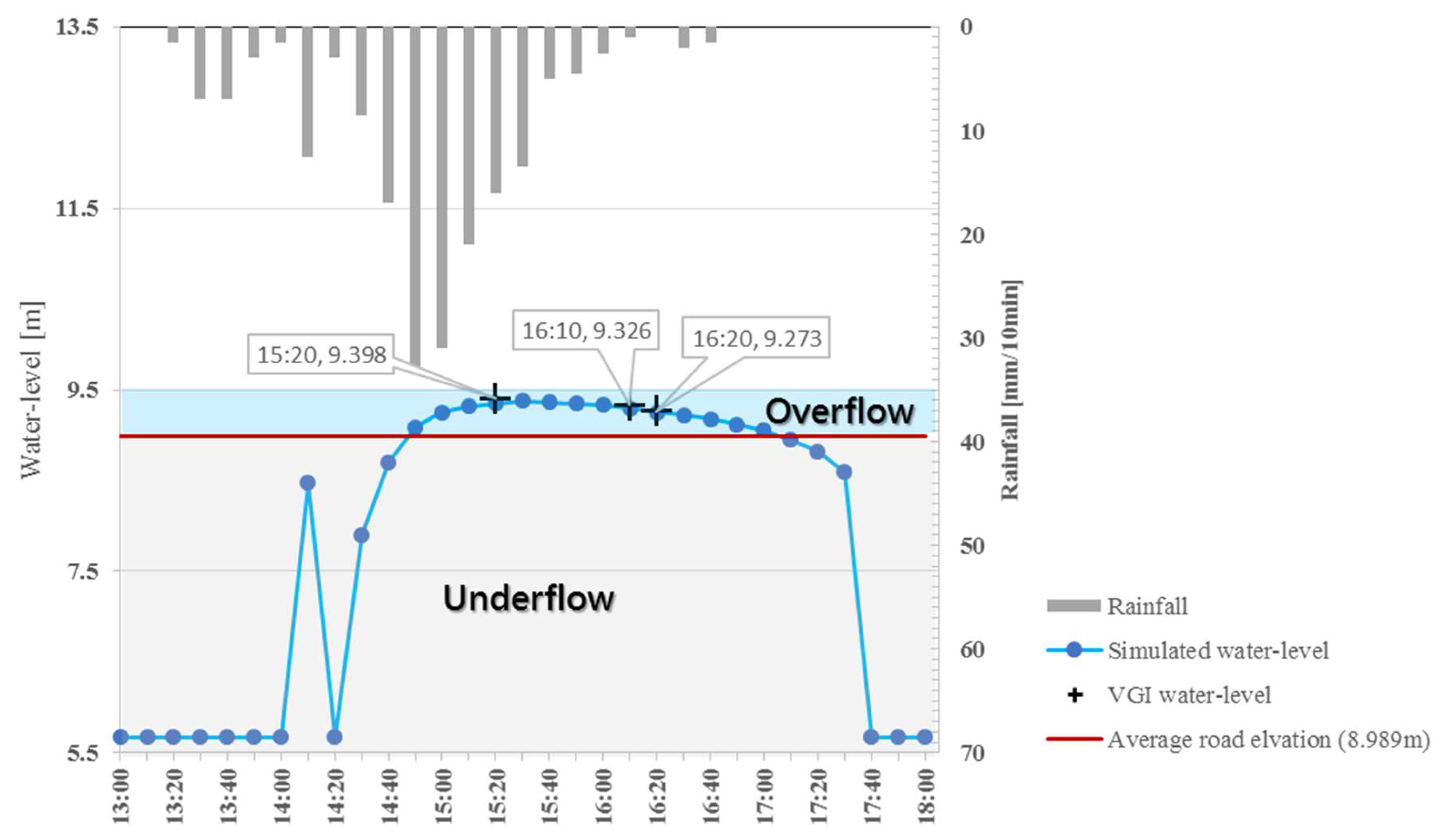
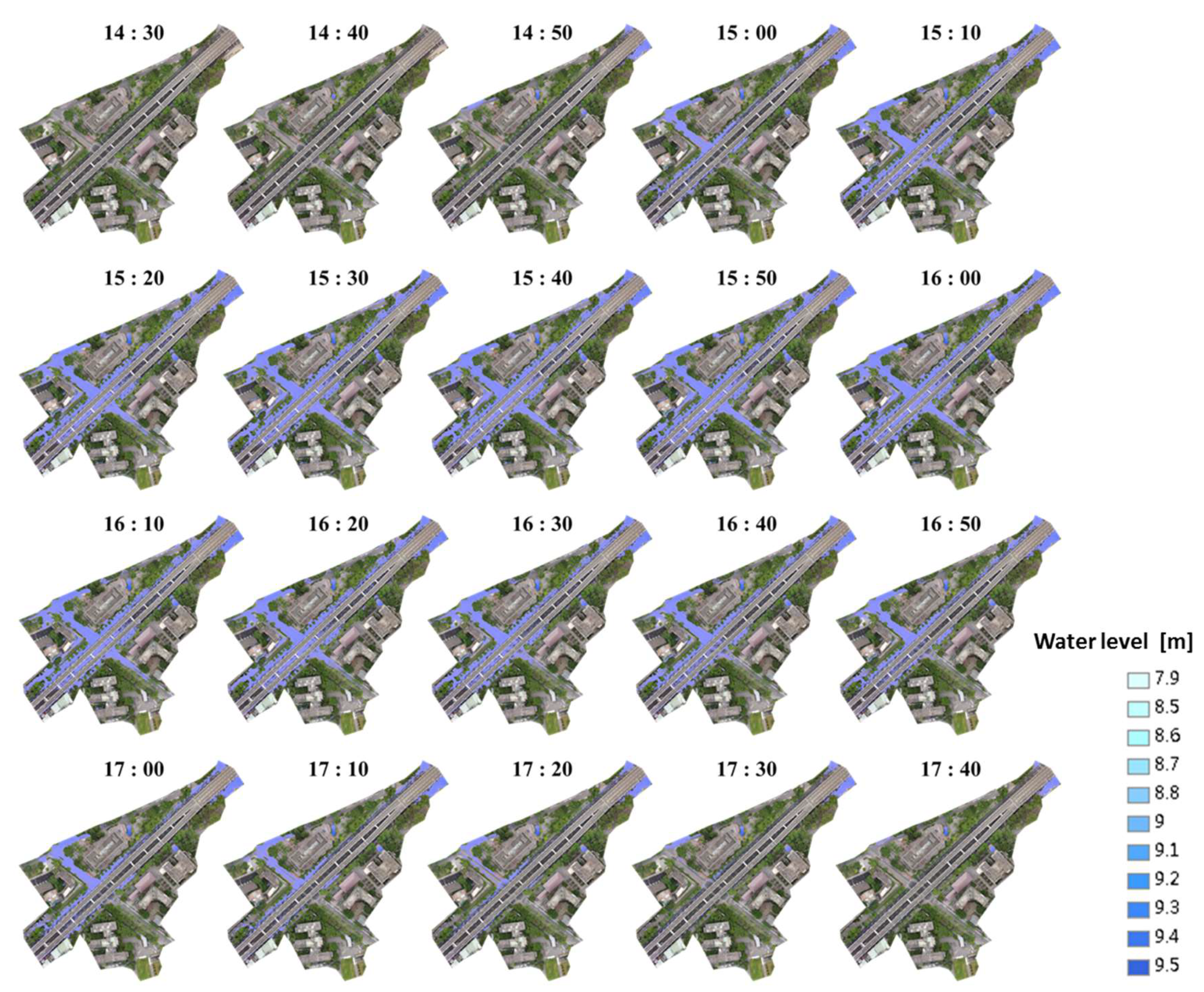
2.3. Rainfall Runoff Simulation to Estimate Flooding Water Level
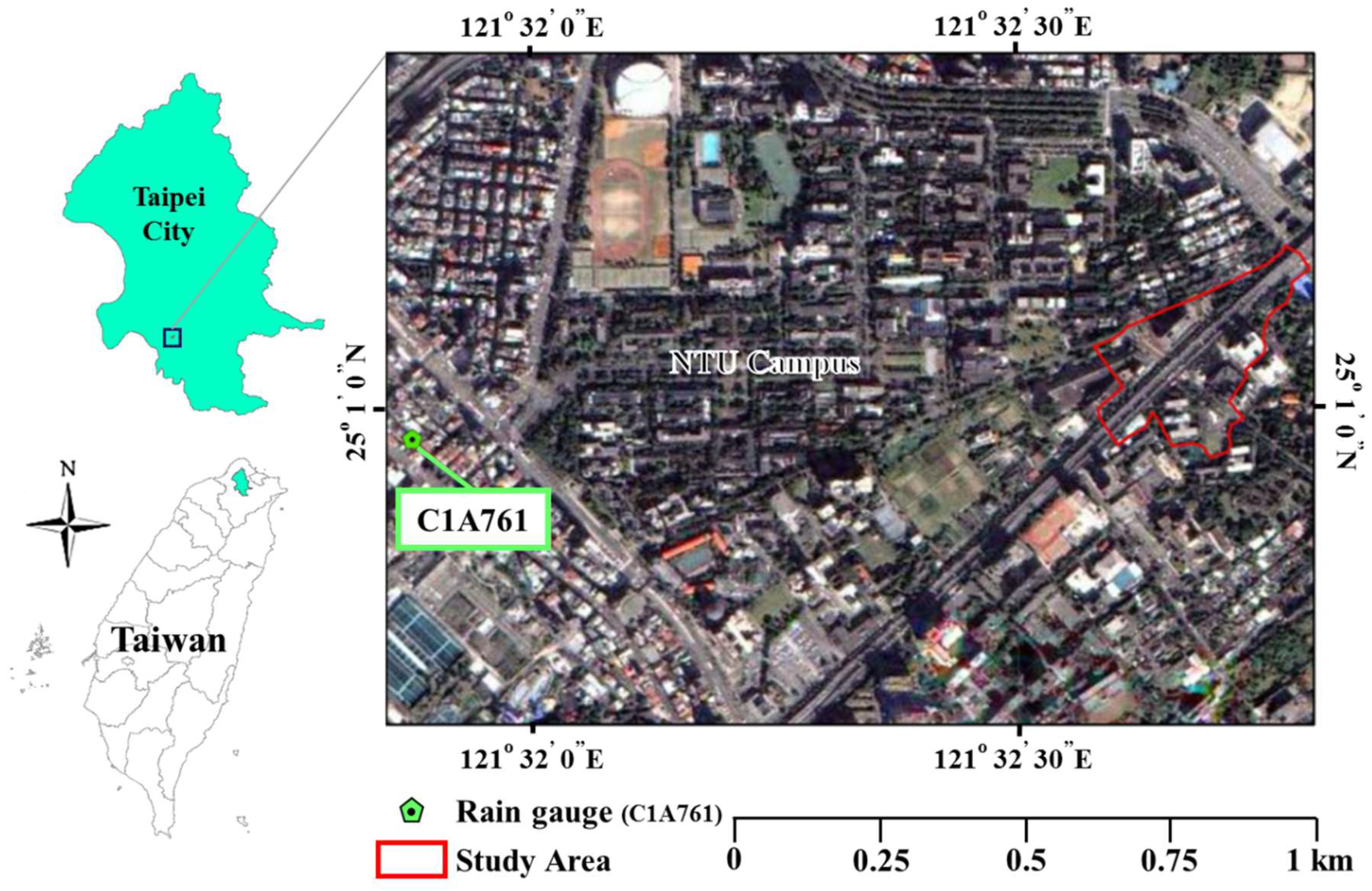
3. Case Study
4. Results
5. Discussion and Conclusions
Author Contributions
Funding
Conflicts of Interest
References
- Panthou, G.; Vischel, T.; Lebel, T. Recent trends in the regime of extreme rainfall in the Central Sahel. Int. J. Climatol. 2014, 34, 3998–4006. [Google Scholar] [CrossRef]
- Bao, J.; Sherwood, S.C.; Alexander, L.V.; Evans, J.P. Future increases in extreme precipitation exceed observed scaling rates. Nat. Clim. Chang. 2017, 7, 128–132. [Google Scholar] [CrossRef]
- Deltares. SOBEK User Manual—Hydrodynamics, Rainfall Runoff and Real Time Control; Deltares: HV Delft, The Netherlands, 2017; pp. 58–73. [Google Scholar]
- Rossman, L.A.; Huber, W.C. Storm Water Management Model Reference Manual Volume I—Hydrology; United States Environmental Protection Agency: Washington, DC, USA, 2016; pp. 20–25. [CrossRef]
- Reed, S.; Schaake, J.; Zhang, Z. A distributed hydrologic model and threshold frequency-based method for flash flood forecasting at ungauged locations. J. Hydrol. 2007, 337, 402–420. [Google Scholar] [CrossRef]
- Norbiato, D.; Borga, M.; Degli Esposti, S.; Gaume, E.; Anquetin, S. Flash flood warning based on rainfall thresholds and soil moisture conditions: An assessment for gauged and ungauged basins. J. Hydrol. 2008, 362, 274–290. [Google Scholar] [CrossRef]
- Neal, J.; Villanueva, I.; Wright, N.; Willis, T.; Fewtrell, T.; Bates, P. How much physical complexity is needed to model flood inundation? Hydrol. Process. 2012, 26, 2264–2282. [Google Scholar] [CrossRef]
- Van der Sande, C.J.; De Jong, S.M.; De Roo, A.P.J. A segmentation and classification approach of IKONOS-2 imagery for land cover mapping to assist flood risk and flood damage assessment. Int. J. Appl. Earth Obs. Geoinf. 2003, 4, 217–229. [Google Scholar] [CrossRef]
- Duncan, J.M.; Biggs, E.M. Assessing the accuracy and applied use of satellite-derived precipitation estimates over Nepal. Appl. Geogr. 2012, 34, 626–638. [Google Scholar] [CrossRef]
- Wood, M.; De Jong, S.M.; Straatsma, M.W. Locating flood embankments using SAR time series: A proof of concept. Int. J. Appl. Earth Obs. Geoinf. 2018, 70, 72–83. [Google Scholar] [CrossRef]
- Yang, M.D.; Yang, Y.F.; Hsu, S.C. Application of remotely sensed data to the assessment of terrain factors affecting Tsao-Ling landside. Can. J. Remote Sens. 2004, 30, 593–603. [Google Scholar] [CrossRef]
- Yang, M.D.; Su, T.C.; Hsu, C.H.; Chang, K.C.; Wu, A.M. Mapping of the 26 December 2004 tsunami disaster by using FORMOSAT-2 images. Int. J. Remote Sens. 2007, 28, 3071–3091. [Google Scholar] [CrossRef]
- Yang, M.D. A genetic algorithm (GA) based automated classifier for remote sensing imagery. Can. J. Remote Sens. 2007, 33, 593–603. [Google Scholar] [CrossRef]
- Blaschke, T.; Hay, G.J.; Weng, Q.; Resch, B. Collective sensing: Integrating geospatial technologies to understand urban systems—An overview. Remote Sens. 2011, 3, 1743–1776. [Google Scholar] [CrossRef]
- Schnebele, E.; Cervone, G. Improving remote sensing flood assessment using volunteered geographical data. Nat. Hazards Earth Syst. Sci. 2013, 13, 669–677. [Google Scholar] [CrossRef]
- Yang, M.D.; Su, T.C.; Lin, H.Y. Fusion of infrared thermal image and visible image for 3D thermal model reconstruction using smartphone sensors. Sensors 2018, 18, 2003. [Google Scholar] [CrossRef]
- Kaplan, A.M.; Haenlein, M. Users of the world, unite! The challenges and opportunities of Social Media. Bus. Horiz. 2010, 53, 59–68. [Google Scholar] [CrossRef]
- Boella, G.; Calafiore, A.; Grassi, E.; Rapp, A.; Sanasi, L.; Schifanella, C. FirstLife: Combining Social Networking and VGI to Create an Urban Coordination and Collaboration Platform. IEEE Access 2019, 7, 63230–63246. [Google Scholar] [CrossRef]
- Longueville, B.D.; Luraschi, G.; Smits, P.; Peedell, S.; Groeve, T.D. Citizens as sensors for natural hazards: A VGI integration workflow. Geomatica 2010, 64, 41–59. [Google Scholar]
- Granell, C.; Ostermann, F.O. Beyond data collection: Objectives and methods of research using VGI and geo-social media for disaster management. Comput. Environ. Urban Syst. 2016, 59, 231–243. [Google Scholar] [CrossRef]
- Vahidi, H.; Klinkenberg, B.; Johnson, B.A.; Moskal, L.M.; Yan, W. Mapping the Individual Trees in Urban Orchards by Incorporating Volunteered Geographic Information and Very High Resolution Optical Remotely Sensed Data: A Template Matching-Based Approach. Remote Sens. 2018, 10, 1134. [Google Scholar] [CrossRef]
- Zamir, A.R.; Shah, M. Accurate image localization based on google maps street view. In European Conference on Computer Vision; Heraklion: Crete, Greece, 2010; pp. 255–268. [Google Scholar] [CrossRef]
- Liang, J.; Gong, J.; Sun, J.; Zhou, J.; Li, W.; Li, Y.; Shen, S. Automatic sky view factor estimation from street view photographs—A big data approach. Remote Sens. 2017, 9, 411. [Google Scholar] [CrossRef]
- Feng, Y.; Sester, M. Extraction of pluvial flood relevant volunteered geographic information (VGI) by deep learning from user generated texts and photos. ISPRS Int. J. Geoinf. 2018, 7, 39. [Google Scholar] [CrossRef]
- Comber, A.; See, L.; Fritz, S.; Van der Velde, M.; Perger, C.; Foody, G. Using control data to determine the reliability of volunteered geographic information about land cover. Int. J. Appl. Earth Obs. Geoinf. 2013, 23, 37–48. [Google Scholar] [CrossRef]
- Foody, G.M.; See, L.; Fritz, S.; Van der Velde, M.; Perger, C.; Schill, C.; Boyd, D.S. Assessing the accuracy of volunteered geographic information arising from multiple contributors to an internet based collaborative project. Trans. GIS 2013, 17, 847–860. [Google Scholar] [CrossRef]
- Fonte, C.C.; Bastin, L.; See, L.; Foody, G.; Lupia, F. Usability of VGI for validation of land cover maps. Int. J. Geogr. Inf. Sci. 2015, 29, 1269–1291. [Google Scholar] [CrossRef]
- Poser, K.; Dransch, D. Volunteered geographic information for disaster management with application to rapid flood damage estimation. Geomatica 2010, 64, 89–98. [Google Scholar]
- Hung, K.C.; Kalantari, M.; Rajabifard, A. Methods for assessing the credibility of volunteered geographic information in flood response: A case study in Brisbane, Australia. Appl. Geogr. 2016, 68, 37–47. [Google Scholar] [CrossRef]
- Kusumo, A.N.L.; Reckien, D.; Verplanke, J. Utilising volunteered geographic information to assess resident’s flood evacuation shelters. Case study: Jakarta. Appl. Geogr. 2017, 88, 174–185. [Google Scholar] [CrossRef]
- Assumpção, T.H.; Popescu, I.; Jonoski, A.; Solomatine, D.P. Citizen observations contributing to flood modelling: Opportunities and challenges. Hydrol. Earth Syst. Sci. 2018, 22, 1473–1489. [Google Scholar] [CrossRef]
- See, L.M. A Review of Citizen Science and Crowdsourcing in Applications of Pluvial Flooding. Front. Earth Sci. 2019, 7, 44. [Google Scholar] [CrossRef]
- Rosser, J.F.; Leibovici, D.G.; Jackson, M.J. Rapid flood inundation mapping using social media, remote sensing and topographic data. Nat. Hazards 2017, 87, 103–120. [Google Scholar] [CrossRef]
- Liu, P.; Chen, A.Y.; Huang, Y.N.; Han, J.Y.; Lai, J.S.; Kang, S.C.; Tsai, M.H. A review of rotorcraft unmanned aerial vehicle (UAV) developments and applications in civil engineering. Smart Struct. Syst. 2014, 13, 1065–1094. [Google Scholar] [CrossRef]
- Mikhail, E.M.; Bethel, J.S.; McGlone, J.C. Introduction to Modern Photogrammetry, 1st ed.; John Wiley and Sons Inc.: Chichester, NY, USA, 2001; p. 237. [Google Scholar]
- Royem, A.A.; Mui, C.K.; Fuka, D.R.; Walter, M.T. Technical note: Proposing a low-tech, affordable, accurate stream stage monitoring system. Trans. ASABE 2012, 55, 2237–2242. [Google Scholar] [CrossRef]
- Lin, F.; Chang, W.Y.; Lee, L.C.; Hsiao, H.T.; Tsai, W.F.; Lai, J.S. Applications of image recognition for real-time water-level and surface velocity. In Proceedings of the 2013 IEEE International Symposium on Multimedia, Anaheim, CA, USA, 9–11 December 2013; pp. 259–262. [Google Scholar] [CrossRef]
- Lin, Y.T.; Lin, Y.C.; Han, J.Y. Automatic water-level detection using single-camera images with varied poses. Measurement 2018, 127, 167–174. [Google Scholar] [CrossRef]
- Yang, M.D.; Su, T.C.; Pan, N.F.; Yang, Y.F. Systematic image quality assessment for sewer inspection. Expert Syst. Appl. 2011, 38, 1766–1776. [Google Scholar] [CrossRef]
- Yang, W.; Tan, R.T.; Feng, J.; Liu, J.; Guo, Z.; Yan, S. Deep joint rain detection and removal from a single image. In Proceedings of the IEEE Conference on Computer Vision and Pattern Recognition, Honolulu, HI, USA, 21–26 July 2017; pp. 1357–1366. [Google Scholar] [CrossRef]
- Yang, M.D.; Su, T.C. Automation model of sewerage rehabilitation planning. Water Sci. Technol. 2006, 54, 225–232. [Google Scholar] [CrossRef] [PubMed]
- Yang, M.D.; Su, T.C.; Pan, N.F.; Liu, P. Feature extraction of sewer pipe defects using wavelet transform and co-occurrence matrix. Int. J. Wavelets Multiresolut. Inf. Process. 2011, 9, 211–225. [Google Scholar] [CrossRef]
- Su, T.C.; Yang, M.D. Application of morphological segmentation to leaking defect detection in sewer pipelines. Sensors 2014, 14, 8686–8704. [Google Scholar] [CrossRef]
- Ma, L.; Li, M.; Ma, X.; Cheng, L.; Du, P.; Liu, Y. A review of supervised object-based land-cover image classification. ISPRS J. Photogramm. Remote Sens. 2017, 130, 277–293. [Google Scholar] [CrossRef]
- Ghosh, A.; Sharma, R.; Joshi, P.K. Random forest classification of urban landscape using Landsat archive and ancillary data: Combining seasonal maps with decision level fusion. Appl. Geogr. 2014, 48, 31–41. [Google Scholar] [CrossRef]
- Li, M.; Ma, L.; Blaschke, T.; Cheng, L.; Tiede, D. A systematic comparison of different object-based classification techniques using high spatial resolution imagery in agricultural environments. Int. J. Appl. Earth Obs. Geoinf. 2016, 49, 87–98. [Google Scholar] [CrossRef]
- Phiri, D.; Morgenroth, J.; Xu, C.; Hermosilla, T. Effects of pre-processing methods on Landsat OLI-8 land cover classification using OBIA and random forests classifier. Int. J. Appl. Earth Obs. Geoinf. 2018, 73, 170–178. [Google Scholar] [CrossRef]
- Tian, S.; Zhang, X.; Tian, J.; Sun, Q. Random forest classification of wetland landcovers from multi-sensor data in the arid region of Xinjiang, China. Remote Sens. 2016, 8, 954. [Google Scholar] [CrossRef]
- Zurqani, H.A.; Post, C.J.; Mikhailova, E.A.; Schlautman, M.A.; Sharp, J.L. Geospatial analysis of land use change in the Savannah River Basin using Google Earth Engine. Int. J. Appl. Earth Obs. Geoinf. 2018, 69, 175–185. [Google Scholar] [CrossRef]
- Breiman, L. Random forests. Mach. Learn. 2001, 45, 5–32. [Google Scholar] [CrossRef]
- Cutler, A.; Cutler, D.R.; Stevens, J.R. Random forests. In Ensemble Machine Learning; Springer: Boston, MA, USA, 2012; pp. 157–175. [Google Scholar] [CrossRef]
- Rodriguez-Galiano, V.F.; Ghimire, B.; Rogan, J.; Chica-Olmo, M.; Rigol-Sanchez, J.P. An assessment of the effectiveness of a random forest classifier for land-cover classification. ISPRS J. Photogramm. Remote Sens. 2012, 67, 93–104. [Google Scholar] [CrossRef]
- Deus, D. Integration of ALOS PALSAR and landsat data for land cover and forest mapping in northern tanzania. Land 2016, 5, 43. [Google Scholar] [CrossRef]
- Tsutsumida, N.; Comber, A.J. Measures of spatio-temporal accuracy for time series land cover data. Int. J. Appl. Earth Obs. Geoinf. 2015, 41, 46–55. [Google Scholar] [CrossRef]
- Yang, M.D.; Huang, K.S.; Wan, J.; Tsai, H.P.; Lin, L.M. Timely and quantitative damage assessment of oyster racks using UAV images. IEEE J. Sel. Top. Appl. Earth Obs. Remote Sens. 2018, 6. [Google Scholar] [CrossRef]
- Batra, B.; Singh, S.; Sharma, J.; Arora, S.M. Computational analysis of edge detection operators. Int. J. Appl. Res. 2016, 2, 257–262. [Google Scholar]
- Li, Y.; Chen, L.; Huang, H.; Li, X.; Xu, W.; Zheng, L.; Huang, J. Nighttime lane markings recognition based on Canny detection and Hough transform. In Proceedings of the 2016 IEEE International Conference on Real-time Computing and Robotics, Angkor Wat, Cambodia, 6–9 June 2016; pp. 411–415. [Google Scholar] [CrossRef]
- Gabriel, E.; Hahmann, F.; Böer, G.; Schramm, H.; Meyer, C. Structured edge detection for improved object localization using the discriminative generalized Hough transform. In Proceedings of the 11th Joint Conference on Computer Vision, Imaging and Computer Graphics Theory and Applications, Rome, Italy, 27–29 February 2016; pp. 393–402. [Google Scholar]
- Deng, G.; Wu, Y. Double Lane Line Edge Detection Method Based on Constraint Conditions Hough Transform. In Proceedings of the 2018 17th International Symposium on Distributed Computing and Applications for Business Engineering and Science (DCABES), Wuxi, China, 19–23 October 2018; pp. 107–110. [Google Scholar] [CrossRef]
- Yang, M.D.; Huang, K.S.; Kuo, Y.H.; Tsai, H.P.; Lin, L.M. Spatial and spectral hybrid image classification for rice-lodging assessment through UAV imagery. Remote Sens. 2017, 9, 583. [Google Scholar] [CrossRef]
- Lampert, D.J.; Wu, M. Development of an open-source software package for watershed modeling with the Hydrological Simulation Program in Fortran. Environ. Model. Softw. 2015, 68, 166–174. [Google Scholar] [CrossRef]
- Chen, C.F.; Liu, C.M. The definition of urban stormwater tolerance threshold and its concept estimation: An example from Taiwan. Nat. Hazards 2014, 73, 173–190. [Google Scholar] [CrossRef]
- Yang, M.D.; Tseng, H.H.; Hsu, Y.C.; Tsai, H.P. Semantic Segmentation Using Deep Learning with Vegetation Indices for Rice Lodging Identification in Multi-date UAV Visible Images. Remote Sens. 2020, 12, 633. [Google Scholar] [CrossRef]


| RF classification | |||||||||
|---|---|---|---|---|---|---|---|---|---|
| 15:20 | 16:10 | 16:20 | |||||||
| User’s accuracy | Producer’s accuracy | F1 Score | User’s accuracy | Producer’s accuracy | F1 Score | User’s accuracy | Producer’s accuracy | F1 Score | |
| Water | 82.55 | 93.32 | 87.61 | 84.41 | 88.72 | 86.51 | 85.66 | 79.78 | 82.61 |
| Vegetation | 76.58 | 78.90 | 77.73 | 82.58 | 82.03 | 82.30 | 88.49 | 86.95 | 87.71 |
| Building | 80.31 | 67.35 | 73.26 | 72.00 | 68.37 | 70.14 | 58.95 | 69.48 | 63.78 |
| Overall accuracy | 80.10 | 80.12 | 79.93 | ||||||
| Kappa coefficient | 70.03 | 70.11 | 68.80 | ||||||
| ML classification | |||||||||
| 15:20 | 16:10 | 16:20 | |||||||
| User’s accuracy | Producer’s accuracy | F1 Score | User’s accuracy | Producer’s accuracy | F1 Score | User’s accuracy | Producer’s accuracy | F1 Score | |
| Water | 80.09 | 81.79 | 80.93 | 77.80 | 86.41 | 81.88 | 77.68 | 67.38 | 72.17 |
| Vegetation | 70.41 | 76.91 | 73.52 | 81.71 | 75.61 | 78.54 | 76.13 | 81.94 | 78.93 |
| Building | 71.08 | 63.95 | 67.33 | 67.19 | 64.21 | 65.66 | 43.94 | 51.63 | 47.48 |
| Overall accuracy | 74.18 | 75.85 | 68.79 | ||||||
| Kappa coefficient | 61.20 | 63.68 | 51.77 | ||||||
| SVM classification | |||||||||
| 15:20 | 16:10 | 16:20 | |||||||
| User’s accuracy | Producer’s accuracy | F1 Score | User’s accuracy | Producer’s accuracy | F1 Score | User’s accuracy | Producer’s accuracy | F1 Score | |
| Water | 80.28 | 86.44 | 83.25 | 81.20 | 86.89 | 83.95 | 81.87 | 71.30 | 76.22 |
| Vegetation | 72.46 | 75.32 | 73.86 | 79.92 | 79.04 | 79.48 | 81.50 | 84.42 | 82.93 |
| Building | 75.73 | 67.15 | 71.18 | 69.98 | 65.29 | 67.55 | 53.51 | 65.79 | 59.02 |
| Overall accuracy | 76.50 | 77.51 | 74.40 | ||||||
| Kappa coefficient | 64.63 | 66.17 | 60.50 | ||||||
| Time | NO. | Object Coordinates | Digital Image Coordinates | |||
|---|---|---|---|---|---|---|
| X [m] | Y [m] | Z [m] | c [pix] | r [pix] | ||
| 15:20 | 1 | 304967.703 | 2767764.523 | 9.342 | 366 | 630 |
| 2 | 304930.212 | 2767771.009 | 20.861 | 493 | 181 | |
| 3 | 304888.931 | 2767800.201 | 23.167 | 750 | 132 | |
| 4 | 304982.202 | 2767780.765 | 19.039 | 1111 | 462 | |
| 5 | 304985.403 | 2767777.323 | 17.207 | 1030 | 652 | |
| 6 | 304968.113 | 2767772.073 | 9.051 | 593 | 620 | |
| 7 | 304949.462 | 2767770.772 | 9.412 | 642 | 455 | |
| 8 | 304953.401 | 2767779.186 | 17.128 | 698 | 301 | |
| 9 | 304959.769 | 2767778.158 | 9.089 | 708 | 511 | |
| 16:10 | 1 | 304883.466 | 2767793.211 | 25.673 | 166 | 197 |
| 2 | 304916.648 | 2767807.092 | 17.152 | 311 | 180 | |
| 3 | 304917.138 | 2767808.913 | 14.081 | 382 | 264 | |
| 4 | 304908.909 | 2767803.371 | 11.312 | 319 | 394 | |
| 5 | 304915.582 | 2767804.933 | 9.218 | 263 | 454 | |
| 6 | 304869.703 | 2767828.152 | 25.313 | 623 | 243 | |
| 7 | 304861.271 | 2767834.319 | 21.512 | 665 | 299 | |
| 8 | 304925.581 | 2767815.242 | 9.141 | 400 | 472 | |
| 9 | 304916.924 | 2767822.723 | 13.183 | 847 | 306 | |
| 16:20 | 1 | 304835.051 | 2767847.961 | 8.801 | 42 | 378 |
| 2 | 304836.242 | 2767849.642 | 8.869 | 31 | 332 | |
| 3 | 304857.942 | 2767869.852 | 12.231 | 124 | 174 | |
| 4 | 304841.014 | 2767851.058 | 8.802 | 194 | 285 | |
| 4 | 304854.977 | 2767868.233 | 8.552 | 100 | 228 | |
| 5 | 304849.758 | 2767850.121 | 9.023 | 426 | 253 | |
| 6 | 304845.532 | 2767844.932 | 8.802 | 550 | 275 | |
| 7 | 304916.336 | 2767861.181 | 22.791 | 575 | 42 | |
| 8 | 304849.412 | 2767846.383 | 9.104 | 569 | 255 | |
| 9 | 304835.053 | 2767847.962 | 8.802 | 42 | 378 | |
| Parameters in Simulation | Value |
|---|---|
| Time interval | 10 min |
| Inundation starting from the lowest grid of the DSM in the study area (A) | 5.670 (m) |
| Discharging rate of sewer system in Taipei City (Q i) | 78.8 (mm/hour) |
| The fitting curve between inundated water volume (S j) and inundated water depth (d) |
| Time | Orientation Parameters | VGI Water-Level h [m] | Simulated Water-Level ĥ [m] | Difference Δh [m] |
|---|---|---|---|---|
| 15:20 | (304999.44, 2767768.66, 26.97, 74.49°, 2.85°, 80.79°, 4.42) | 9.398 | 9.353 | 0.045 |
| 16:10 | (304940.476, 2767809.813, 10.43, 92.82°, 1.72°, 85.37°, 4.49) | 9.326 | 9.296 | 0.030 |
| 16:20 | (304828.98, 2767839.16, 3.62, 62.45°, 5.16°, 124.33°, 5.67) | 9.273 | 9.255 | 0.018 |
© 2020 by the authors. Licensee MDPI, Basel, Switzerland. This article is an open access article distributed under the terms and conditions of the Creative Commons Attribution (CC BY) license (http://creativecommons.org/licenses/by/4.0/).
Share and Cite
Lin, Y.-T.; Yang, M.-D.; Han, J.-Y.; Su, Y.-F.; Jang, J.-H. Quantifying Flood Water Levels Using Image-Based Volunteered Geographic Information. Remote Sens. 2020, 12, 706. https://doi.org/10.3390/rs12040706
Lin Y-T, Yang M-D, Han J-Y, Su Y-F, Jang J-H. Quantifying Flood Water Levels Using Image-Based Volunteered Geographic Information. Remote Sensing. 2020; 12(4):706. https://doi.org/10.3390/rs12040706
Chicago/Turabian StyleLin, Yan-Ting, Ming-Der Yang, Jen-Yu Han, Yuan-Fong Su, and Jiun-Huei Jang. 2020. "Quantifying Flood Water Levels Using Image-Based Volunteered Geographic Information" Remote Sensing 12, no. 4: 706. https://doi.org/10.3390/rs12040706
APA StyleLin, Y.-T., Yang, M.-D., Han, J.-Y., Su, Y.-F., & Jang, J.-H. (2020). Quantifying Flood Water Levels Using Image-Based Volunteered Geographic Information. Remote Sensing, 12(4), 706. https://doi.org/10.3390/rs12040706