Construction of Nighttime Cloud Layer Height and Classification of Cloud Types

 ,
, 


Abstract
1. Introduction
2. Sensors and Data
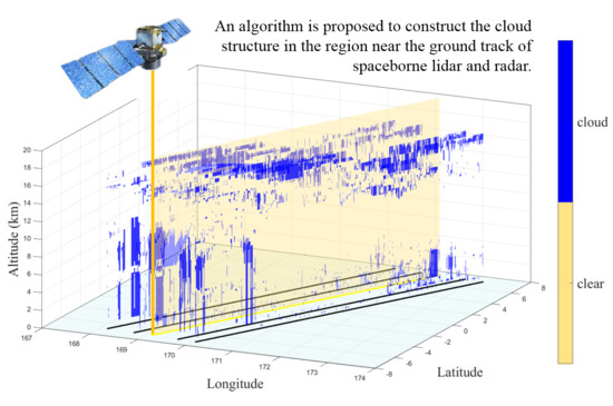
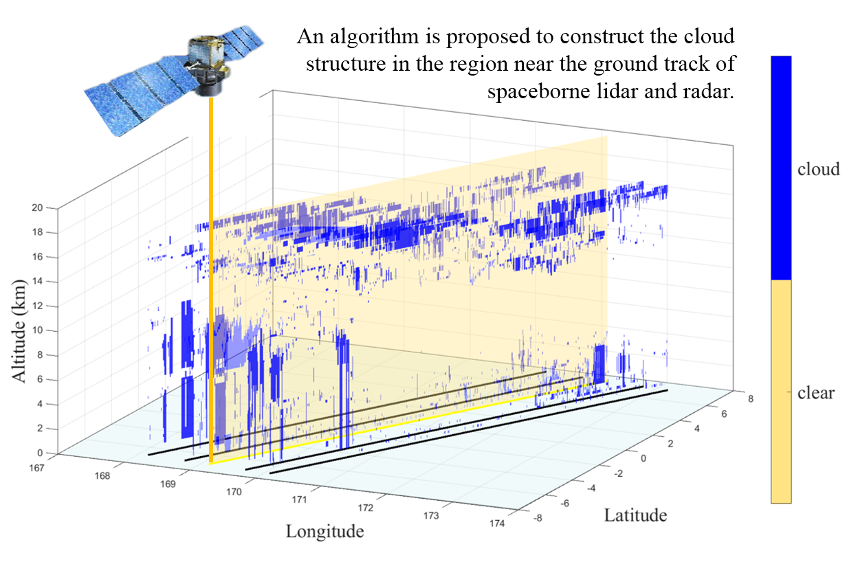
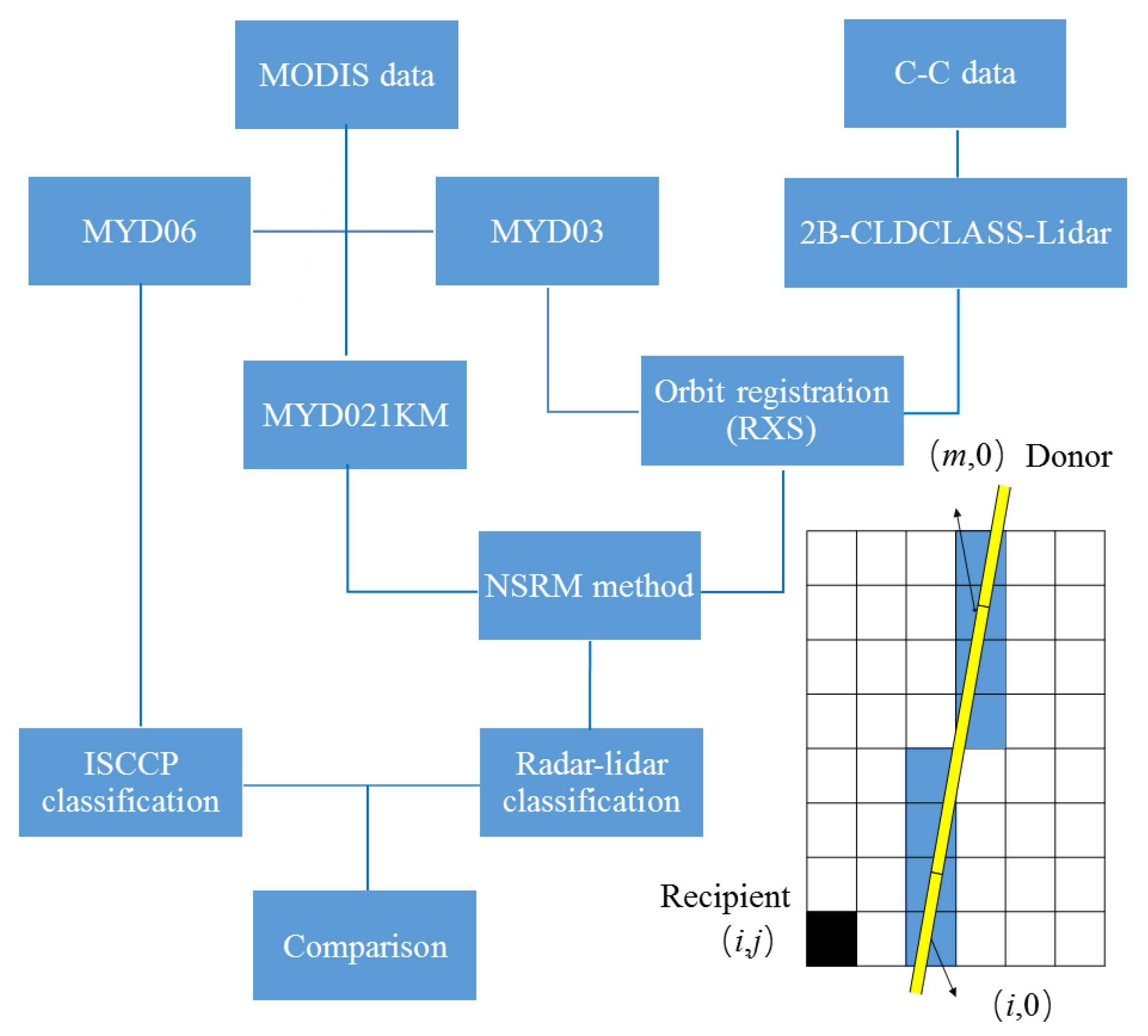
3. Method
- (1)
- The potential donors must have the same surface type as the recipient. The surface type of each pixel is obtained from the MYD03 land/sea mask product.
- (2)
- The potential donors must be similar enough in their solar positions to the recipient. The difference of both solar zenith angles and solar azimuth angles need to be negligible.
- (3)
- The potential donors must have the same cloud scenario as the recipient, which means they are either both cloudy or both clear in the MYD06 cloud mask flags.
- (4)
- Based on the availability, potential donors should ideally have sufficiently small uncertainties with their retrieved properties.
4. Results and Discussion
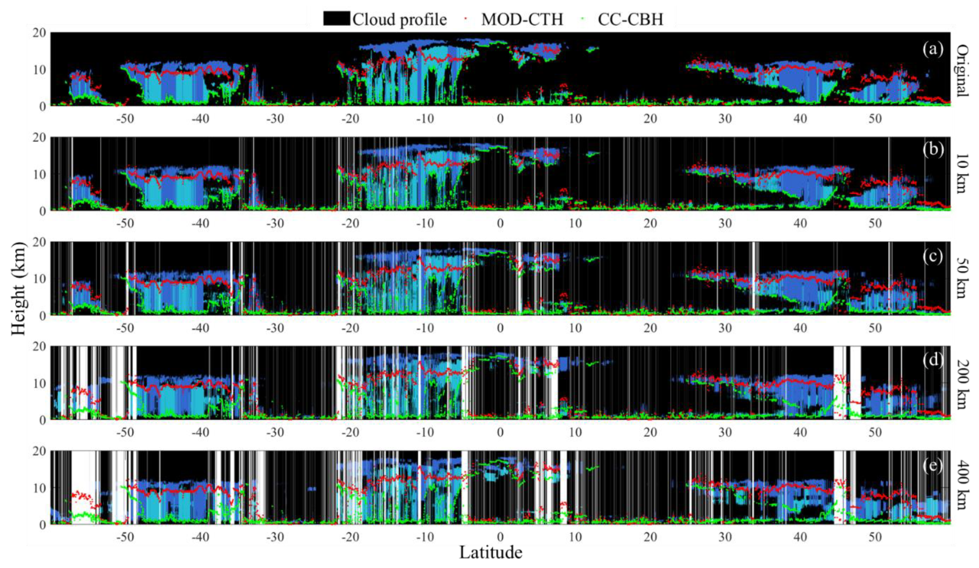
4.1. Performance of the NSRM Method
4.2. Nighttime Cloud Classification
4.3. Daytime Verification of the Cloud Classification Results
5. Conclusions
Author Contributions
Funding
Acknowledgments
Conflicts of Interest
References
- IPCC. Contribution of Working Group I to the Fifth Assessment Report of the Intergovernmental Panel on Climate Change. In Climate Change 2013: The Physical Science Basis; Stocker, T.F., Qin, D., Plattner, G.-K., Tignor, M., Allen, S.K., Boschung, J., Nauels, A., Xia, Y., Bex, V., Midgley, P.M., Eds.; Cambridge University Press: Cambridge, UK; New York, NY, USA, 2013; p. 1535. [Google Scholar] [CrossRef]
- Stubenrauch, C.J.; Rossow, W.B.; Kinne, S.; Ackerman, S.; Cesana, G.; Chepfer, H.; Di Girolamo, L.; Getzewich, B.; Guignard, A.; Heidinger, A.; et al. Assessment of Global Cloud Datasets from Satellites: Project and Database Initiated by the GEWEX Radiation Panel. Bull. Am. Meteorol. Soc. 2013, 94, 1031–1049. [Google Scholar] [CrossRef]
- Ramanathan, V.; Cess, R.D.; Harrison, E.F.; Minnis, P.; Barkstrom, B.R.; Ahmad, E.; Hartmann, D. Cloud-Radiative forcing and climate-Results from the earth radiation budget experiment. Science 1989, 243, 57–63. [Google Scholar] [CrossRef] [PubMed]
- Rossow, W.B.; Garder, L.C.; Lacis, A.A. Global, Seasonal Cloud Variations from Satellite Radiance Measurements. Part I: Sensitivity of Analysis. J. Clim. 1989, 2, 419–458. [Google Scholar] [CrossRef]
- Rossow, W.B.; Schiffer, R.A. Advances in understanding clouds from ISCCP. Bull. Am. Meteorol. Soc. 1999, 80, 2261–2287. [Google Scholar] [CrossRef]
- Wind, G.; Platnick, S.; King, M.D.; Hubanks, P.A.; Pavolonis, M.J.; Heidinger, A.K.; Yang, P.; Baum, B.A. Multilayer Cloud Detection with the MODIS Near-Infrared Water Vapor Absorption Band. J. Appl. Meteorol. Climatol. 2010, 49, 2315–2333. [Google Scholar] [CrossRef]
- Minnis, P.; Sun-Mack, S.; Young, D.F.; Heck, P.W.; Garber, D.P.; Chen, Y.; Spangenberg, D.A.; Arduini, R.F.; Trepte, Q.Z.; Smith, W.L., Jr.; et al. CERES Edition-2 Cloud Property Retrievals Using TRMM VIRS and Terra and Aqua MODIS Data-Part I: Algorithms. IEEE Trans. Geosci. Remote Sens. 2011, 49, 4374–4400. [Google Scholar] [CrossRef]
- Foga, S.; Scaramuzza, P.L.; Guo, S.; Zhu, Z.; Dilley, R.D., Jr.; Beckmann, T.; Schmidt, G.L.; Dwyer, J.L.; Hughes, M.J.; Laue, B. Cloud detection algorithm comparison and validation for operational Landsat data products. Remote Sens. Environ. 2017, 194, 379–390. [Google Scholar] [CrossRef]
- Pavolonis, M.J. Advances in Extracting Cloud Composition Information from Spaceborne Infrared Radiances-A Robust Alternative to Brightness Temperatures. Part I: Theory. J. Appl. Meteorol. Climatol. 2010, 49, 1992–2012. [Google Scholar] [CrossRef]
- Baum, B.A.; Menzel, W.P.; Frey, R.A.; Tobin, D.C.; Holz, R.E.; Ackerman, S.A.; Heidinger, A.K.; Yang, P. MODIS Cloud-Top Property Refinements for Collection 6. J. Appl. Meteorol. Climatol. 2012, 51, 1145–1163. [Google Scholar] [CrossRef]
- Shonk, J.K.P.; Hogan, R.J.; Manners, J. Impact of improved representation of horizontal and vertical cloud structure in a climate model. Clim. Dyn. 2012, 38, 2365–2376. [Google Scholar] [CrossRef]
- Pincus, R.; Hemler, R.; Klein, S.A. Using stochastically generated subcolumns to represent cloud structure in a large-scale model. Mon. Weather Rev. 2006, 134, 3644–3656. [Google Scholar] [CrossRef]
- Stephens, G.L.; Vane, D.G.; Boain, R.J.; Mace, G.G.; Sassen, K.; Wang, Z.E.; Illingworth, A.J.; O′Connor, E.J.; Rossow, W.B.; Durden, S.L.; et al. The cloudsat mission and the a-train-A new dimension of space-Based observations of clouds and precipitation. Bull. Am. Meteorol. Soc. 2002, 83, 1771–1790. [Google Scholar] [CrossRef]
- Winker, D.M.; Vaughan, M.A.; Omar, A.; Hu, Y.X.; Powell, K.A.; Liu, Z.Y.; Hunt, W.H.; Young, S.A. Overview of the CALIPSO Mission and CALIOP Data Processing Algorithms. J. Atmos. Ocean. Technol. 2009, 26, 2310–2323. [Google Scholar] [CrossRef]
- Kim, S.W.; Berthier, S.; Raut, J.C.; Chazette, P.; Dulac, F.; Yoon, S.C. Validation of aerosol and cloud layer structures from the space-borne lidar CALIOP using a ground-based lidar in Seoul, Korea. Atmos. Chem. Phys. 2008, 8, 3705–3720. [Google Scholar] [CrossRef]
- Vaughan, M.A.; Powell, K.A.; Kuehn, R.E.; Young, S.A.; Winker, D.M.; Hostetler, C.A.; Hunt, W.H.; Liu, Z.; McGill, M.J.; Getzewich, B.J. Fully Automated Detection of Cloud and Aerosol Layers in the CALIPSO Lidar Measurements. J. Atmos. Ocean. Technol. 2009, 26, 2034–2050. [Google Scholar] [CrossRef]
- Platnick, S.; King, M.D.; Ackerman, S.A.; Menzel, W.P.; Baum, B.A.; Riedi, J.C.; Frey, R.A. The MODIS cloud products: Algorithms and examples from Terra. IEEE Trans. Geosci. Remote Sens. 2003, 41, 459–473. [Google Scholar] [CrossRef]
- Barker, H.W.; Jerg, M.P.; Wehr, T.; Kato, S.; Donovan, D.P.; Hogan, R.J. A 3D cloud-Construction algorithm for the EarthCARE satellite mission. Q. J. R. Meteorol. Soc. 2011, 137, 1042–1058. [Google Scholar] [CrossRef]
- Miller, S.D.; Forsythe, J.M.; Partain, P.T.; Haynes, J.M.; Bankert, R.L.; Sengupta, M.; Mitrescu, C.; Hawkins, J.D.; Vonder Haar, T.H. Estimating Three-Dimensional Cloud Structure via Statistically Blended Satellite Observations. J. Appl. Meteorol. Climatol. 2014, 53, 437–455. [Google Scholar] [CrossRef]
- Forsythe, J.M.; Vonder Haar, T.H.; Reinke, D.L. Cloud-Base height estimates using a combination of meteorological satellite imagery and surface reports. J. Appl. Meteorol. 2000, 39, 2336–2347. [Google Scholar] [CrossRef]
- Hutchison, K.; Wong, E.; Ou, S.C. Cloud base heights retrieved during night-Time conditions with MODIS data. Int. J. Remote Sens. 2006, 27, 2847–2862. [Google Scholar] [CrossRef]
- Sun, X.J.; Li, H.R.; Barker, H.W.; Zhang, R.W.; Zhou, Y.B.; Liu, L. Satellite-Based estimation of cloud-Base heights using constrained spectral radiance matching. Q. J. R. Meteorol. Soc. 2016, 142, 224–232. [Google Scholar] [CrossRef]
- Noh, Y.-J.; Forsythe, J.M.; Miller, S.D.; Seaman, C.J.; Li, Y.; Heidinger, A.K.; Lindsey, D.T.; Rogers, M.A.; Partain, P.T. Cloud-Base Height Estimation from VIIRS. Part II: A Statistical Algorithm Based on A-Train Satellite Data. J. Atmos. Ocean. Technol. 2017, 34, 585–598. [Google Scholar] [CrossRef]
- Liu, D.; Chen, S.; Cheng, C.; Barker, H.W.; Dong, C.; Ke, J.; Wang, S.; Zheng, Z. Analysis of global three-Dimensional aerosol structure with spectral radiance matching. Atmos. Meas. Tech. 2019, 12, 6541–6556. [Google Scholar] [CrossRef]
- Li, H.R.; Sun, X.J. Retrieving cloud base heights via the combination of CloudSat and MODIS observations. In Proceedings of the Conference on Remote Sensing of the Atmosphere, Clouds, and Precipitation V, Beijing, China, 13–15 October 2014. [Google Scholar]
- Hutchison, K.D. The retrieval of cloud base heights from MODIS and three-Dimensional cloud fields from NASA′s EOS Aqua mission. Int. J. Remote Sens. 2002, 23, 5249–5265. [Google Scholar] [CrossRef]
- Chand, D.; Anderson, T.L.; Wood, R.; Charlson, R.J.; Hu, Y.; Liu, Z.; Vaughan, M. Quantifying above-Cloud aerosol using spaceborne lidar for improved understanding of cloudy-Sky direct climate forcing. J. Geophys. Res.-Atmos. 2008, 113. [Google Scholar] [CrossRef]
- Savtchenko, A.; Kummerer, R.; Smith, P.; Kempler, S.; Leptoukh, G. A-Train Data Depot-Bringing Atmospheric Measurements Together. IEEE Trans. Geosci. Remote Sens. 2008, 46, 2788–2795. [Google Scholar] [CrossRef]
- Wang, H.; Xu, X. Cloud Classification in Wide-Swath Passive Sensor Images Aided by Narrow-Swath Active Sensor Data. Remote Sens. 2018, 10, 812. [Google Scholar] [CrossRef]
- Ackerman, S.A.; Strabala, K.I.; Menzel, W.P.; Frey, R.A.; Moeller, C.C.; Gumley, L.E. Discriminating clear sky from clouds with MODIS. J. Geophys. Res.-Atmos. 1998, 103, 32141–32157. [Google Scholar] [CrossRef]
- Baum, B.A.; Soulen, P.F.; Strabala, K.I.; King, M.D.; Ackerman, S.A.; Menzel, W.P.; Yang, P. Remote sensing of cloud properties using MODIS airborne simulator imagery during SUCCESS 2. Cloud thermodynamic phase. J. Geophys. Res.-Atmos. 2000, 105, 11781–11792. [Google Scholar] [CrossRef]
- Barker, H.W.; Cole, J.N.S.; Shephard, M.W. Estimation of errors associated with the EarthCARE 3D scene construction algorithm. Q. J. R. Meteorol. Soc. 2014, 140, 2260–2271. [Google Scholar] [CrossRef]
- Marchant, B.; Platnick, S.; Meyer, K.; Arnold, G.T.; Riedi, J. MODIS Collection 6 shortwave-Derived cloud phase classification algorithm and comparisons with CALIOP. Atmos. Meas. Tech. 2016, 9, 1587–1599. [Google Scholar] [CrossRef]
- Platnick, S.; Meyer, K.G.; King, M.D.; Wind, G.; Amarasinghe, N.; Marchant, B.; Arnold, G.T.; Zhang, Z.; Hubanks, P.A.; Holz, R.E.; et al. The MODIS Cloud Optical and Microphysical Products: Collection 6 Updates and Examples From Terra and Aqua. IEEE Trans. Geosci. Remote Sens. 2017, 55, 502–525. [Google Scholar] [CrossRef] [PubMed]
- Chan, M.A.; Comiso, J.C. Cloud features detected by MODIS but not by CloudSat and CALIOP. Geophys. Res. Lett. 2011, 38. [Google Scholar] [CrossRef]


© 2020 by the authors. Licensee MDPI, Basel, Switzerland. This article is an open access article distributed under the terms and conditions of the Creative Commons Attribution (CC BY) license (http://creativecommons.org/licenses/by/4.0/).
Share and Cite
Chen, S.; Cheng, C.; Zhang, X.; Su, L.; Tong, B.; Dong, C.; Wang, F.; Chen, B.; Chen, W.; Liu, D. Construction of Nighttime Cloud Layer Height and Classification of Cloud Types. Remote Sens. 2020, 12, 668. https://doi.org/10.3390/rs12040668
Chen S, Cheng C, Zhang X, Su L, Tong B, Dong C, Wang F, Chen B, Chen W, Liu D. Construction of Nighttime Cloud Layer Height and Classification of Cloud Types. Remote Sensing. 2020; 12(4):668. https://doi.org/10.3390/rs12040668
Chicago/Turabian StyleChen, Sijie, Chonghui Cheng, Xingying Zhang, Lin Su, Bowen Tong, Changzhe Dong, Fu Wang, Binglong Chen, Weibiao Chen, and Dong Liu. 2020. "Construction of Nighttime Cloud Layer Height and Classification of Cloud Types" Remote Sensing 12, no. 4: 668. https://doi.org/10.3390/rs12040668
APA StyleChen, S., Cheng, C., Zhang, X., Su, L., Tong, B., Dong, C., Wang, F., Chen, B., Chen, W., & Liu, D. (2020). Construction of Nighttime Cloud Layer Height and Classification of Cloud Types. Remote Sensing, 12(4), 668. https://doi.org/10.3390/rs12040668