A Sparse Representation-Based Sample Pseudo-Labeling Method for Hyperspectral Image Classification

Abstract

Hyperspectral image classification methods may not achieve good performance when a limited number of training samples are provided. However, labeling sufficient samples of hyperspectral images to achieve adequate training is quite expensive and difficult. In this paper, we propose a novel sample pseudo-labeling method based on sparse representation (SRSPL) for hyperspectral image classification, in which sparse representation is used to select the purest samples to extend the training set. The proposed method consists of the following three steps. First, intrinsic image decomposition is used to obtain the reflectance components of hyperspectral images. Second, hyperspectral pixels are sparsely represented using an overcomplete dictionary composed of all training samples. Finally, information entropy is defined for the vectorized sparse representation, and then the pixels with low information entropy are selected as pseudo-labeled samples to augment the training set. The quality of the generated pseudo-labeled samples is evaluated based on classification accuracy, i.e., overall accuracy, average accuracy, and Kappa coefficient. Experimental results on four real hyperspectral data sets demonstrate excellent classification performance using the new added pseudo-labeled samples, which indicates that the generated samples are of high confidence.

1. Introduction

Hyperspectral images (HSIs) have hundreds of spectral bands that contain detailed spectral information. Thus, hyperspectral images are widely used in precision agriculture [1], geological prospecting [2], target detection [3], and landscape classification [4]. Classification is one of the important branches in hyperspectral image processing [5] because it can help people understand hyperspectral image scenes via visual classification. However, in the context of supervised classification, the existence of the “Hughes phenomenon” [6] caused by an imbalance between the limited training samples and the extreme spectral dimension of hyperspectral images influences the classification performance [7].

To alleviate the “Hughes phenomenon”, dimensionality reduction [8,9] and semi-supervised classification [10,11] have been extensively studied. The former can reduce the dimensions of hyperspectral images, and the latter can increase the number of training samples. In general, the dimension reduction method can be divided into two categories: feature extraction and feature selection. Among them, feature extraction [12,13] reduces computational complexity by projecting high-dimensional data into low-dimensional data space, and feature selection [14] selects appropriate bands from the original set of spectral bands. In addition to the dimensionality reduction method, semi-supervised classification is often used in the case of small samples. For example, graph-based [15,16], active learning-based [17,18], and generative model-based [19,20] methods have attracted the attention of researchers seeking to tackle the problems caused by the limited availability of labeled samples. These semi-supervised methods can compensate for the lack of labeled samples and improve the classification results.

Pseudo-labeled sample generation is also a commonly used method for semi-supervised classification, which attempts to assign pseudo-labels to more samples. In [21], a combination of active learning (AL) and semi-supervised learning (SSL) is used in a novel manner to obtain more pseudo-labeled samples. In [22], high-confidence semi-labeled samples whose class labels are determined by an ML classifier are added to the training samples to improve hyperspectral image classification performance. In [23], a constrained Dirichlet process mixture model is proposed that produces high-quality pseudo-labels for unlabeled data. In [24], a sifting generative adversarial networks is used to generate more numerous, more diverse, and more authentic labeled samples for data augmentation. However, active learning requires manual intervention, and other methods require multiple iterations or deep learning to converge.

In recent years, sparse representation-based classification (SRC) methods have drawn much attention in dealing with small training sample problems in hyperspectral image classification [25,26]. The goal of SRC is to represent an unknown sample compactly using only a small number of atoms in an overcomplete dictionary. The class label with the minimal representative error will be assigned to the unlabeled samples. Some researchers extended the SRC-based methods to utilize spatial information in hyperspectral images, e.g., joint SRC [27,28], kernel SRC [29,30,31], adaptive SRC [32,33], etc. In addition, there was also some work that used multi-objective optimization to improve SRC directly [34,35]. Ideally, the nonzero elements in a sparse representation vector will be associated with atoms of a single class in the dictionary, and we can easily assign a test sample to that class.

Motivated by sparse representation, a novel sparse representation-based sample pseudo-labeling (SRSPL) method is proposed. In the field of remote sensing, if a pixel contains only one type of land cover, this pixel is called a pure pixel; otherwise, it is a mixed pixel. Due to the limitation of the spatial resolution of the imaging spectrometers, the problem of mixed pixels is quite common in hyperspectral remote sensing images [36]. In general, for the mixed pixels of HSIs, the sparse representation of their spectral features usually involves multiple classes, so the representation coefficient vectors have larger entropies. Conversely, for the pure pixels of HSIs, the spectral features can be linearly represented using atoms from a single class in the overcomplete dictionary, so the representation coefficient vectors of pure pixels will have smaller entropies. Thus, the pixels with small sparse representation entropies can be used to augment the training samples. Using this method, the size of the training sample set can be effectively increased. However, due to factors such as illumination, shading, and noise, the spectral features of different land covers in natural scenes are usually subject to some degree of distortion. Consequently, the generated pseudo-labeled samples cannot guarantee a high quality when the sparse representation method is applied to the hyperspectral pixels. To solve this problem, the intrinsic image decomposition (IID) [37] method is used in this paper before generating samples to extract the spectral reflectance components of the original hyperspectral image. The classification accuracy on four HSIs verifies that the pseudo-labeled samples generated by the proposed method are of high quality.

The main innovations of the proposed SRSPL method are summarized as follows:

1. The information entropy of sparse representation coefficient vectors is first used in the training sample generation of HSIs. The SRC method will assign class labels with minimal sparse representation errors for hyperspectral pixels other than training samples and test samples. However, we only select pixels with small class uncertainty as pseudo-labeled samples to augment the original training set.

2. We have found that, for HSI, remote sensing reflectance extraction is necessary before using the sparse representation method. In this paper, the effective IID method is performed on the HSI, which is beneficial for reducing the sparse representation error.

The experimental results illustrate that the proposed method for pseudo-labeled sample generation based on sparse representation is very effective in improving the classification results.

The remainder of this paper is organized as follows. Related work is described in Section 2. The proposed SRSPL method is introduced in Section 3. The experiment are presented in Section 4. Discussion and conclusions are provided in Section 5 and Section 6, respectively.

2. Related Work

2.1. Intrinsic Image Decomposition of Hyperspectral Images

Intrinsic image decomposition (IID) [37] is a challenging problem in computer vision that aims at modeling the perceiving function of human vision to distinguish the reflectance and shading of the objects from a single image [38]. Since the intrinsic components of an image reflect different physical characteristics of the scene, e.g., reflectance, illumination, and shading, many issues such as natural image segmentation [39] can benefit from IID. Given a single RGB image $\mathbf{G}$, the IID algorithm decomposes $\mathbf{G}$ into two components: the spectral reflectance component $\mathbf{R}$ and the shading component $\mathbf{S}$:

$$\mathbf{G}=\mathbf{RS}$$

(1)

We denote each pixel $i\in \mathbf{G}$ as ${\mathbf{G}}_i={\mathbf{R}}_i{\mathit{S}}_i$, where ${\mathbf{G}}_i=({\mathbf{G}}_{ir},{\mathbf{G}}_{ig},{\mathbf{G}}_{ib})$ and ${\mathbf{R}}_i=({\mathbf{R}}_{ir},{\mathbf{R}}_{ig},{\mathbf{R}}_{ib})$. The parameters r, g, and b refer to the red, green, and blue channels of a color image, respectively.

The optimization-based IID [40] method is based on the assumption of the local color characteristics in images; in a local window of an image, the changes in pixel values are usually caused by changes in the reflectance [41]. Under this assumption, the shading component could be separated from the input image. Thus, the reflectance value of one pixel can be represented by the weighted summation of its neighborhood pixel values:

$${\mathbf{R}}_i=\sum _{j\in N\left(i\right)}{w}_{ij}{\mathbf{R}}_j,w_{ij}=e^{-{({\mathbf{Y}}_i-{\mathbf{Y}}_j)}^2/2{\sigma }_{i\mathbf{Y}}^2+\mathcal{A}{({\mathbf{G}}_i,{\mathbf{G}}_j)}^2/{\sigma }_{i\mathit{A}}^2}$$

(2)

where $N\left(i\right)$ is the set of neighboring pixels around pixel i; $w_{ij}$ measures the similarity of the intensity value and the spectral angle value between pixel i and pixel j; $\mathbf{Y}$ represents the intensity image, which is calculated by averaging all the image bands; ${\mathbf{R}}_j=({\mathbf{R}}_{jr},{\mathbf{R}}_{jg},{\mathbf{R}}_{jb})$, $\mathcal{A}({\mathbf{G}}_i,{\mathbf{G}}_j)=\mathrm{arcos}({\mathbf{G}}_{ir}{\mathbf{G}}_{jr}+{\mathbf{G}}_{ig}{\mathbf{G}}_{jg}+{\mathbf{G}}_{ib}{\mathbf{G}}_{jb})$ denote the angle between the pixel vectors ${\mathbf{G}}_i$ and ${\mathbf{G}}_j$; and ${\sigma }_{i\mathbf{Y}}$, ${\sigma }_{i\mathbf{A}}$ denote the variance of the intensities and the angle in a local window around i, respectively.

Based on Equations (1) and (2), the shading component $\mathbf{S}$ and the reflectance component $\mathbf{R}$ can be obtained by optimizing the following energy function:

$$E(\mathbf{G},\mathbf{R},\mathbf{S})=\sum _{i\in \mathbf{G}}{({\mathbf{R}}_i-\sum _{j\in N\left(i\right)}{w}_{ij}{\mathbf{R}}_j)}^2+\sum _{i\in \mathbf{G}}(\frac{{\mathbf{G}}_i}{{\mathbf{S}}_i}-{\mathbf{R}}_i{)}^2$$

(3)

The complete description of the optimized process can be found in [40].

Kang et al. [37] first extended the IID as a feature extraction method from a three-band image to a hyperspectral image (HSI) of more than 100 bands and achieved excellent results. Here, the pixel values of HSIs are determined by the spectral reflectance, which is determined by the material of different objects, and the shading component, which consists of light and shape-dependent properties. The shading component is not directly related to the material of the object. Therefore, IID is adopted to extract the spectral reflectance components of the HSI to distinguish more classes, and remove useless spatial information preserved in the shading component of the HSIs.

2.2. Sparse Representation Classification of Hyperspectral Images

The sparse representation classification (SRC) framework was first introduced for face recognition [42]. Chen et al. [43] extended the SRC to pixelwise HSI classification, which relied on the observation that spectral pixels of a particular class should lie in a low-dimensional subspace spanned by dictionary atoms (training pixels) from the same class. An unknown test pixel can be represented as a linear combination of training pixels from all classes. For HSI classification, suppose that we have C distinct classes and stack an overcomplete dictionary $\mathit{A}=[{\mathit{A}}_1,{\mathit{A}}_2,\dots ,{\mathit{A}}_N]\in {\mathbb{R}}^{B\times N}$, where B denotes the number of bands and N is the number of training samples, respectively. Set $\mathcal{L}\in \{1,2,\dots ,C\}$ is a set of labels, and $c\in \mathcal{L}$ refers to the cth class. For a test sample $x\in {\mathbb{R}}^{B\times 1}$ of HSI, $x$ can be represented as follows:

$$x={\mathit{A}}_1{\mathit{\alpha }}_1+{\mathit{A}}_2{\mathit{\alpha }}_2+\cdots +{\mathit{A}}_N{\mathit{\alpha }}_N=\mathit{A}\mathit{\alpha }$$

(4)

where $\mathit{\alpha }={[{\mathit{\alpha }}_1,{\mathit{\alpha }}_2,\dots ,{\mathit{\alpha }}_N]}^T\in {\mathbb{R}}^B$ represents the sparse vector. Intuitively, the sparse vector $\mathit{\alpha }$ can be measured by the $l_0$-norm of it ($l_0$-norm counts the number of nonzero entries in a vector). Since the combinatorial $l_0$-norm minimization is an NP-hard problem, the $l_1$-norm minimization, as the closest convex function to $l_0$-norm minimization, is widely employed in sparse coding, and it was shown that $l_0$-norm and $l_1$-norm minimizations are equivalent if the solution is sufficiently sparse [44].

As the hyperspectral signals from the same class often span the same low-dimensional subspace that is constructed by the corresponding training samples, which involves the non-zero entries of the sparse vector, the class of the hyperspectral signal $x$ can be directly determined by the characteristics of the recovered sparse vector $\mathit{\alpha }$. Given the dictionary of training samples $\mathit{A}$, the sparse representation coefficient vector $\mathit{\alpha }$ can be be recovered by solving the following Lasso problem:

$$\widehat{\mathit{\alpha }}=\underset{\mathit{\alpha }}{min}\frac{1}{2}{∥x-\mathit{A}\mathit{\alpha }∥}_2^2+\lambda {∥\mathit{\alpha }∥}_1$$

(5)

where ${∥·∥}_2$ represents the $l_2$ norm, ${∥·∥}_1$ represents the $l_1$ norm of the vector and $\lambda >0$ is a scalar regularization parameter. This optimization problem can be solved by Proximal Gradient Descent (PGD) [45]. After the sparse representation vector $\widehat{\mathit{\alpha }}$ is obtained, the label of the test sample $x$ of HSI can be assigned by the minimal reconstructed residual:

$${\widehat{y}}_x=arg\underset{c=1,\dots ,C}{min}{∥x-{\mathit{A}}^c{\widehat{\mathit{\alpha }}}^c∥}_2^2$$

(6)

where ${\mathit{A}}^c$ is the subdictionary of the cth class and ${\widehat{\mathit{\alpha }}}^c$ denotes the representative coefficient of the cth class.

3. Proposed Method

A novel sparse representation-based sample pseudo-labeling (SRSPL) method is proposed in this paper. The SRSPL method consists of the following three steps. First, IID is used to reduce the dimension and noise of the original hyperspectral image. Second, sparse representation is applied to generate the sparse representation vectors of the hyperspectral pixels other than the training samples and test samples. The information entropies of all these hyperspectral pixels are calculated based on the sparse representation vectors to discriminate purity, and the samples with low representation entropies are selected to generate candidate samples. Third, these candidate samples are assigned pseudo-labels by the minimal reconstructed residual. Then, these pseudo-labeled samples are augmented to the original training set, and an extended random walker (ERW) classifier is trained to evaluate the sample quality. Figure 1 shows a graphical example illustrating the principle of the proposed SRSPL method.

3.1. Feature Extraction of Hyperspectral Images

(1) Spectral Dimensionality Reduction

The initial hyperspectral image $\mathbf{I}=(I_1,\dots ,I_N)\in {\mathbb{R}}^{B\times N}$ is divided into M groups of equal band sizes [37], where N is the number of pixels and B is the dimension of the initial image. The number of bands in each group is denoted by $B_1,B_2,\dots ,B_M$.

The averaging-based image fusion is applied to each group and the resulting fused bands are used for further processing:

$${\tilde{\mathbf{I}}}_m=\frac{{\sum }_{n=1}^{B_m}{\mathbf{I}}_m^n}{B_m}$$

(7)

where m is the mth group, ${\mathbf{I}}_m^n$ is the nth band in the mth group of the original hyperspectral data, $B_m$ is the number of bands in the mth group, and ${\tilde{\mathbf{I}}}_m$ is the mth fused band. Here, the averaging-based method can ensure that the pixels of the dimensionality-reduced hyperspectral image can still be directly interpreted in a physical sense. In other words, the pixels of the dimensionality-reduced image will be related to the reflectance of the scene. Moreover, this method can effectively remove image noise.

(2) Band Grouping

The dimensionality-reduced image $\tilde{\mathbf{I}}$ is partitioned into several subgroups of adjacent bands as follows:

$$\begin{array}{c}\hfill {\widehat{\mathbf{I}}}^k=\left\{\begin{array}{cc}({\tilde{\mathbf{I}}}_{(k-1)Z+1},\dots ,{\tilde{\mathbf{I}}}_{(k-1)Z+Z}),\hfill & \hfill k=1,2,\dots ,\lfloor M/Z\rfloor \\ ({\tilde{\mathbf{I}}}_{M-Z+1},\dots ,{\tilde{\mathbf{I}}}_M),\hfill & \hfill k=\lceil M/Z\rceil \ne \lfloor M/Z\rfloor \end{array}\right.\end{array}$$

(8)

where ${\widehat{\mathbf{I}}}^k$ refers to the kth subgroup, $\lfloor M/Z\rfloor$ is the largest integer not greater than $M/Z$, and $\lceil M/Z\rceil$ is the smallest integer not less than $M/Z$. Here, Z refers to the number of bands in each subgroup.

(3) Reflectance Extraction with the Optimization-Based IID

For each subgroup ${\widehat{\mathbf{I}}}^k$, the optimization-based IID method is used to obtain the reflectance and shading components, and the equation is as follows:

$$({\mathbf{R}}^{k^{*}},{\mathbf{S}}^{k^{*}})=arg\underset{{\mathbf{R}}^k,{\mathbf{S}}^k}{min}E({\widehat{\mathbf{I}}}^k,{\mathbf{R}}^k,{\mathbf{S}}^k)$$

(9)

where ${\mathbf{R}}^k$ and ${\mathbf{S}}^k$ refer to the reflectance and the shading components of the kth subgroup, respectively.

The reflectance components of the different subgroups are combined to obtain the resulting IID features, which is an M-dimensional feature matrix $\tilde{\mathbf{R}}$ that can be used for subsequent processing.

$$\tilde{\mathbf{R}}=\left(\begin{array}{c}{\mathbf{R}}^1\\ \dots \\ {\mathbf{R}}^k\\ \dots \\ {\mathbf{R}}^{\lceil M/Z\rceil }\end{array}\right)\in {\mathbb{R}}^{M\times N}$$

(10)

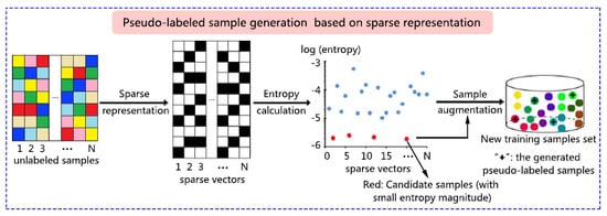
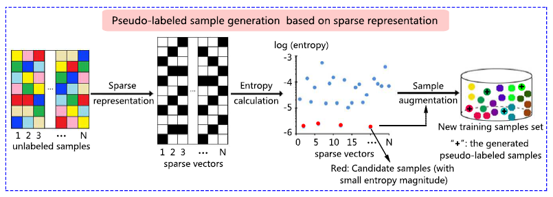
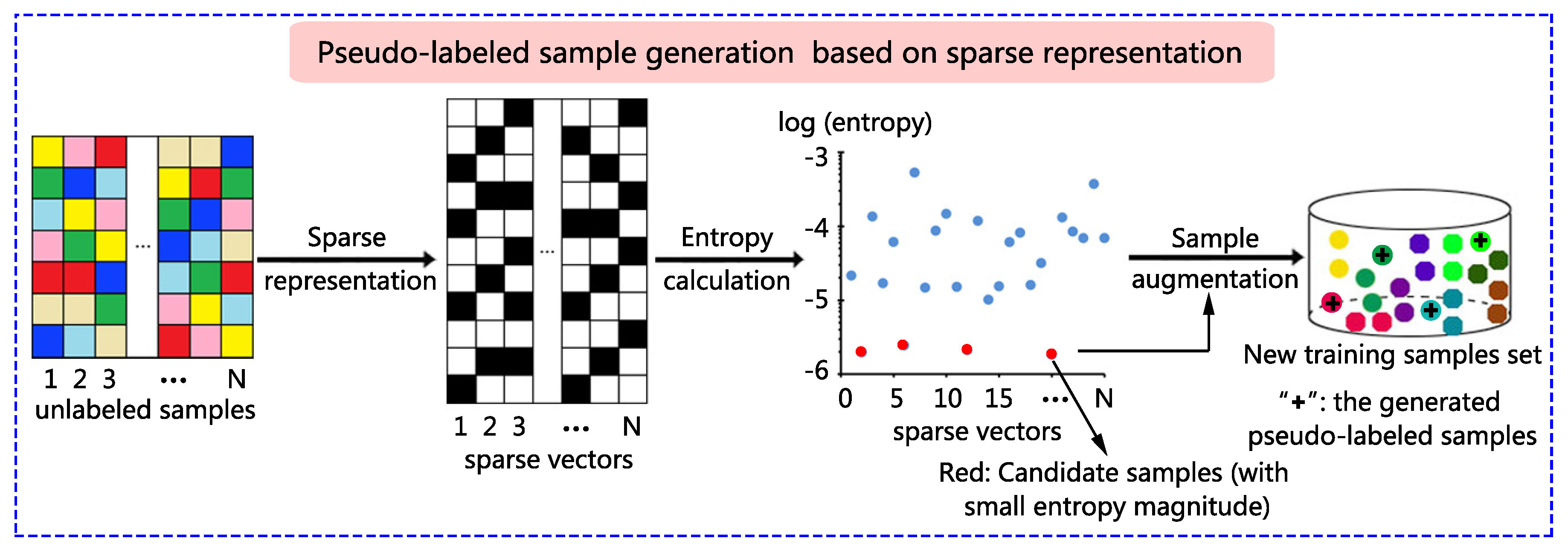
3.2. Candidate Sample Selection Based on Sparse Representation

To find the purest pixels and use them as candidate samples, we first calculate the sparse representation of all the hyperspectral samples other than the training samples and test them (denoted as ${\mathit{S}}_{unlabeled}={\left({\mathit{I}}_i\right)}_{i=1}^u$). Then, we determine the purity of the samples by calculating its sparse representation information entropy. When a sample has a lower sparse representation information entropy, it is very likely to be a pure pixel. The process can be described as follows:

(1) Calculating the Hyperspectral Sample’s Sparse Representation

For a given sample ${\mathit{I}}_i\in {\mathit{S}}_{unlabeled}$, ${\tilde{\mathbf{R}}}_{{\mathit{I}}_i}$ denotes the reflectance component of ${\mathit{I}}_i$, and ${\tilde{\mathbf{R}}}_{{\mathit{I}}_i}\in {\mathbb{R}}^M$. The goal of sparse representation is to represent ${\tilde{\mathbf{R}}}_{{\mathit{I}}_i}$ by a sparse linear combination of training samples that make up the dictionary. Suppose $\mathcal{L}\in \{1,2,\dots ,C\}$ is a set of labels and $c\in \mathcal{L}$ refers to the cth class. The representation coefficient $\tilde{\mathit{\alpha }}$ of ${\tilde{\mathbf{R}}}_{I_i}$ can be calculated based on an overcomplete dictionary $\tilde{\mathit{A}}$ according to Equation (5). Therefore, ${\tilde{\mathbf{R}}}_{{\mathit{I}}_i}$ is assumed to lie in the union of the C different subspaces, which can be seen as the sparse linear combination of all the training samples:

$$\begin{array}{cc}\hfill {\tilde{\mathbf{R}}}_{{\mathit{I}}_i}& ={\tilde{\mathit{A}}}^1{\tilde{\mathit{\alpha }}}^1+{\tilde{\mathit{A}}}^2{\tilde{\mathit{\alpha }}}^2+···+{\tilde{\mathit{A}}}^C{\tilde{\mathit{\alpha }}}^C\hfill \\ \hfill & =\left[{\tilde{\mathit{A}}}^1\cdots {\tilde{\mathit{A}}}^C\right]\left[\begin{array}{c}\hfill {\tilde{\mathit{\alpha }}}^1\\ \hfill \cdots \\ \hfill {\tilde{\mathit{\alpha }}}^C\end{array}\right]=\tilde{\mathit{A}}\tilde{\mathit{\alpha }}\hfill \end{array}$$

(11)

where $\tilde{\mathit{A}}\in {\mathbb{R}}^{M\times N_m}$ is the structured overcomplete dictionary, which consists of the class sub-dictionaries ${\left\{{\tilde{\mathit{A}}}^c\right\}}_{c=1,\dots ,C}$. $N_m$ is the number of training samples, and $\tilde{\mathit{\alpha }}$ is an $N_m$-dimensional representation coefficient vector formed by concatenating the sparse vectors ${\left\{{\tilde{\mathit{\alpha }}}^c\right\}}_{c=1,\dots ,C}$.

The representation coefficient $\tilde{\mathit{\alpha }}$ of ${\tilde{\mathbf{R}}}_{{\mathit{I}}_i}$ can be recovered by solving the following optimization problem:

$$\tilde{\mathit{\alpha }}=\underset{\tilde{\mathit{\alpha }}}{min}\frac{1}{2}{∥{\tilde{\mathbf{R}}}_{{\mathit{I}}_i}-\tilde{\mathit{A}}\tilde{\mathit{\alpha }}∥}_2^2+\lambda {∥\tilde{\mathit{\alpha }}∥}_1$$

(12)

where $\lambda$ is a scalar regularization parameter and requires experimental analysis to determine the optimal value.

(2) Discriminating the Purity of Hyperspectral Samples based on Information Entropy

The information entropy of each ${\tilde{\mathbf{R}}}_{{\mathit{I}}_i}$ is calculated based on its representation coefficient:

$$\mathrm{Ent}\left({\tilde{\mathbf{R}}}_{{\mathit{I}}_i}\right)=-\sum _{j=1}^{N_m}{\tilde{\mathit{\alpha }}}_j\log \left({\tilde{\mathit{\alpha }}}_j\right)$$

(13)

where $\mathrm{Ent}(·)$ denotes an entropy function and $\tilde{\mathit{\alpha }}$ is the representation coefficient vector of ${\tilde{\mathbf{R}}}_{{\mathit{I}}_i}$. The purity of ${\tilde{\mathbf{R}}}_{{\mathit{I}}_i}$ is determined according to the magnitude of the entropy.

(3) Finding the Candidate Samples

First, the information entropy for the reflectance components of each ${\tilde{\mathbf{R}}}_{{\mathit{I}}_i}$ is obtained. Second, these samples corresponding to these reflectance components are sorted in ascending order according to the magnitude of their entropies. Third, the first T samples are selected as the candidate samples set ${\mathit{S}}_{candidate}={\left({\tilde{\mathbf{R}}}_{{\mathit{I}}_i}\right)}_{i=1}^T$, where the parameter T is an optimal value obtained by experiments.

3.3. Pseudo-Label Assignment for Candidate Samples

For each candidate sample, one pseudo-label is determined based on the minimal reconstructed residual:

$${\tilde{y}}_{{\mathit{I}}_i}=arg\underset{c=1,\dots ,C}{min}{∥{\tilde{\mathbf{R}}}_{{\mathit{I}}_i}-{\tilde{\mathit{A}}}^c{\tilde{\mathit{\alpha }}}^c∥}_2^2$$

(14)

where ${\tilde{\mathit{A}}}^c$ is the sub-dictionary of the cth class and ${\tilde{\mathit{\alpha }}}^c$ denotes the representative coefficient of the cth class. Thus, the pseudo-labeled sample set is ${\mathit{S}}_{pseudo}={({\tilde{\mathbf{R}}}_{{\mathit{I}}_i},{\tilde{y}}_{I_i})}_{i=1}^T$.

3.4. Classification Model Optimization Using Pseudo-Labeled Samples

First, the pseudo-labeled samples set ${\mathit{S}}_{pseudo}$ and the initial labeled samples set ${\mathit{S}}_{initial}$ are combined to form the new labeled samples set ${\mathit{S}}_{labeled}$. Then, the ERW [46] algorithm is used as a classification model to evaluate the quality of these newly generated pseudo-labeled samples, where the ERW algorithm is adopted to calculate a set of optimized probabilities for the class of each pixel to be determined based on the maximum probability.

3.5. Pseudo-Code of the Proposed SRSPL Method

For a detailed illustration of the proposed SRSPL method, the pseudocode of the proposed SRSPL method is shown in Algorithm 1.

Algorithm 1: Sparse Representation-based Sample Pseudo-Labeling (SRSPL) for Hyperspectral Image

Classification

Input: Hyperspectral image $\mathbf{I}=({\mathit{I}}_1,\dots ,{\mathit{I}}_N)$; the initial labeled samples set ${\mathit{S}}_{initial}={({\mathit{I}}_i,y_i)}_{i=1}^l$; the hyper-

spectral samples set other than the training samples and test samples: ${\mathit{S}}_{unlabeled}={\left(I_i\right)}_{i=1}^u$

Output: Classification map $\mathrm{C}$

1: Reduce the dimension and noise of $\mathbf{I}$ based on averaging image fusion (Equation (7)) to obtain the

dimensionally reduced image $\tilde{\mathbf{I}}$.

2: According to Equation (8), partition the $\tilde{\mathbf{I}}$ into several subgroups of adjacent bands, denoted as ${\widehat{\mathbf{I}}}^k$.

3: According to Equations (9) and (10), obtain the spectral reflectance components of each ${\widehat{\mathbf{I}}}^k$, (through the

optimization-based IID method) and combined to obtain the resulting IID features $\tilde{\mathbf{R}}$.

4: For each ${\mathit{I}}_i,i=1:u({\mathit{I}}_i\in {\mathit{S}}_{unlabeled})$ Do

(1) According to Equation (11) and (12), solve the sparse representation coefficient $\tilde{\mathit{\alpha }}$ of each sample ${\mathit{I}}_i$

based on the reflectance component ${\tilde{\mathbf{R}}}_{{\mathit{I}}_i}$ and the overcomplete dictionary $\tilde{\mathit{A}}$.

(2) According to Equation (13), calculate the information entropy of each ${\tilde{\mathbf{R}}}_{{\mathit{I}}_i}$ to discriminating the

purity of each sample ${\mathit{I}}_i$.

5:End For

6: Sort the samples corresponding to these reflectance components in ascending order according to their

entropy magnitudes.

7: Selected the first T samples as the candidate samples set ${\mathit{S}}_{candidate}={\left({\tilde{\mathbf{R}}}_{I_i}\right)}_{i=1}^T$.

8: According to Equation (14), assign the pseudo-label for each sample in set ${\mathit{S}}_{candidate}$, to obtain the pseudo-

labeled samples set ${\mathit{S}}_{pseudo}={({\tilde{\mathbf{R}}}_{{\mathit{I}}_i},{\tilde{y}}_{{\mathit{I}}_i})}_{i=1}^T$.

9: Combine the initial labeled samples set ${\mathit{S}}_{initial}$ and the pseudo-labeled samples set ${\mathit{S}}_{pseudo}$ to the new

labeled samples set ${\mathit{S}}_{labeled}$.

10: Classify the spectral reflectance components $\tilde{\mathbf{R}}$ with the extended random walker (ERW) classifier and the

new labeled samples set ${\mathit{S}}_{labeled}$ to obtain the final classification map $\mathrm{C}$.

11:Return$\mathrm{C}$

4. Experiment

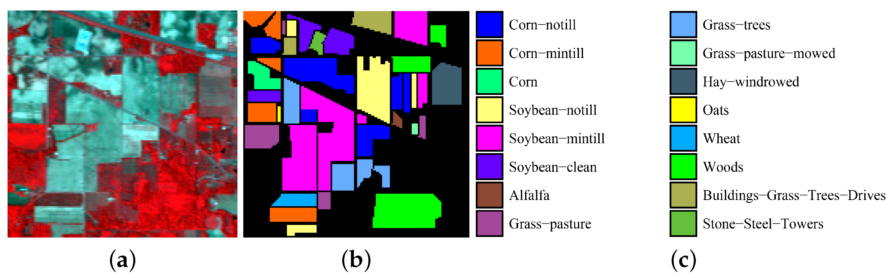
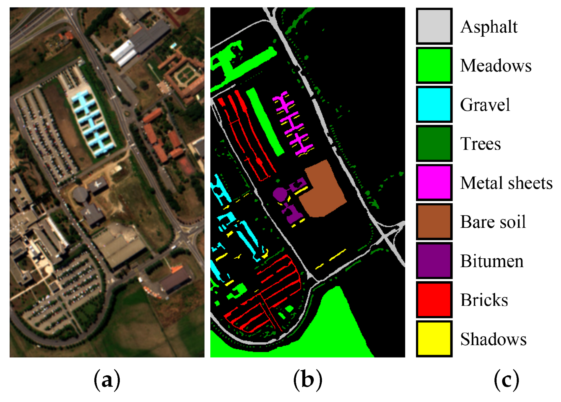
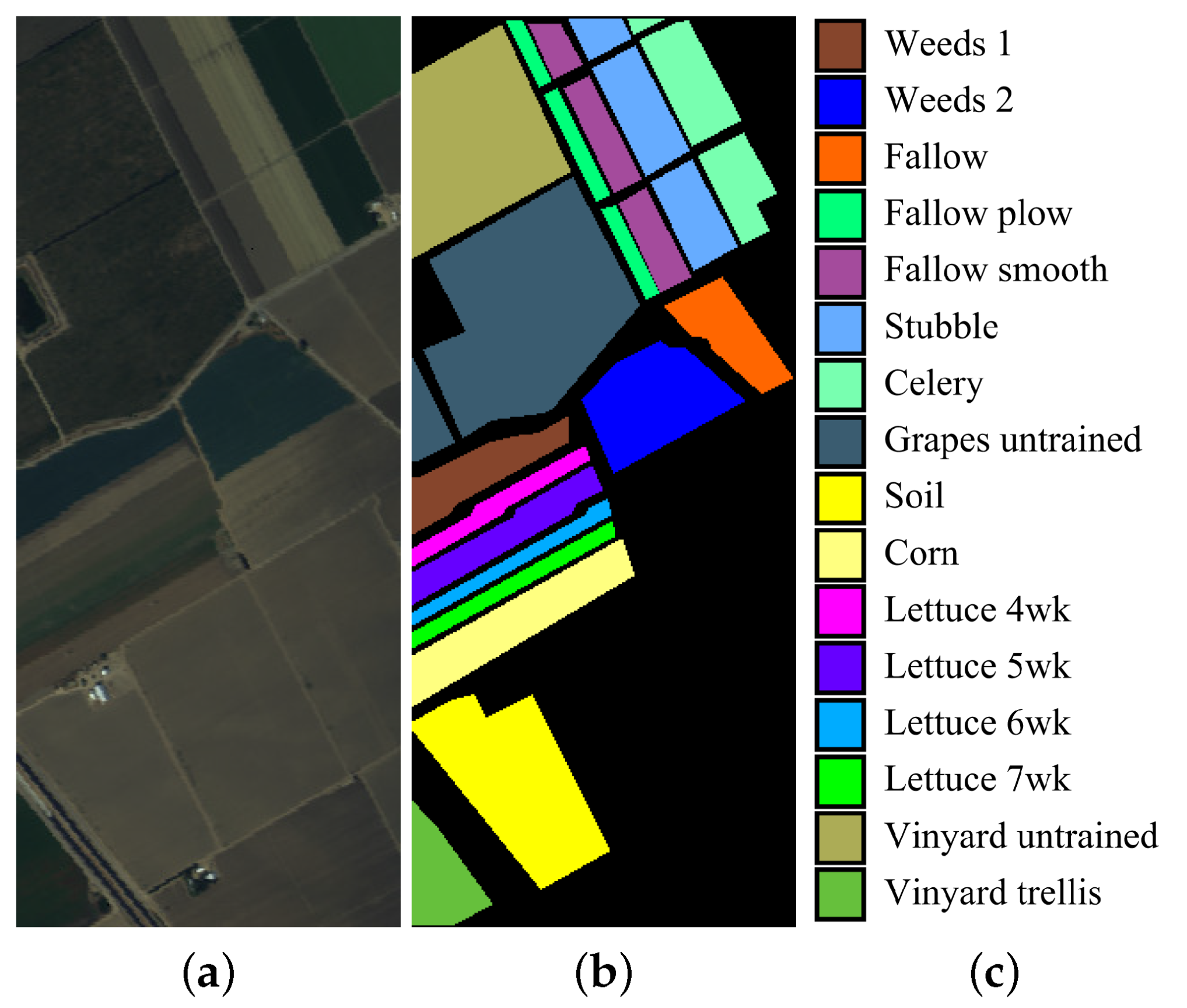
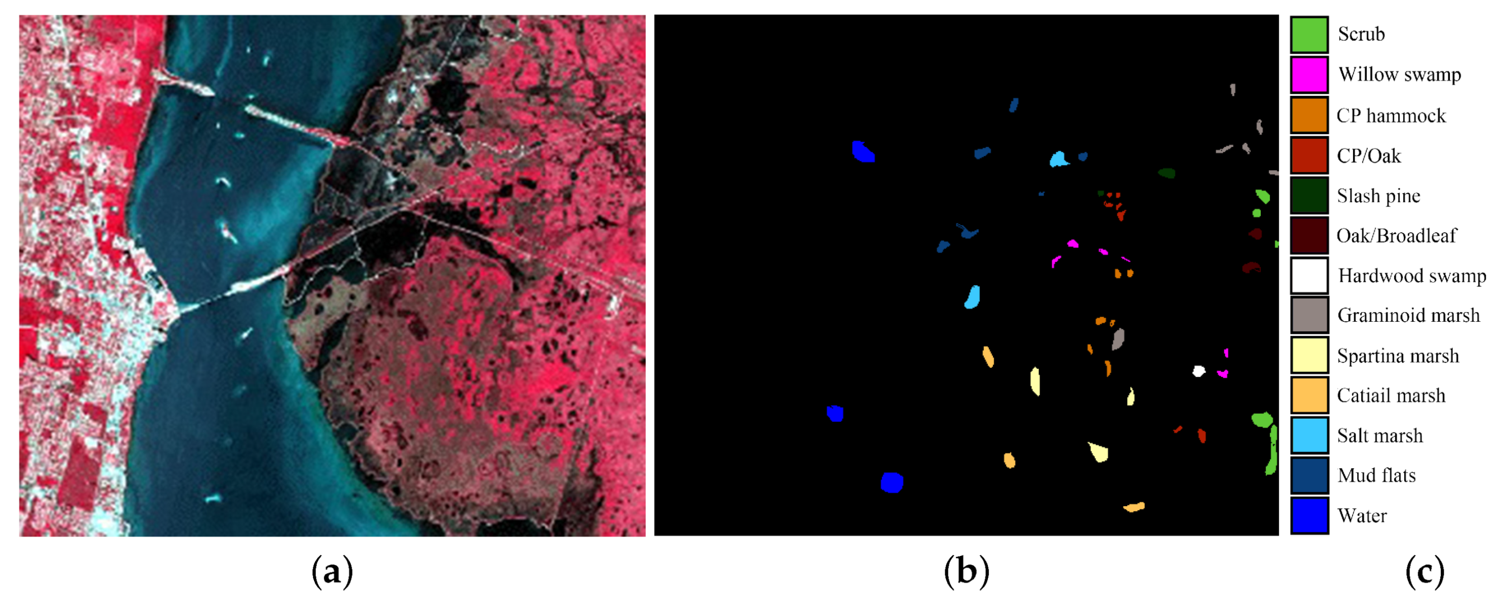
4.1. Experimental Data Sets

(1) Indian Pines data set: The Indian Pines image was acquired by the Airborne Visible/Infrared Imaging Spectrometer (AVIRIS) sensor, which captured the Indian Pines unlabeled agricultural site in northwestern Indiana. The image contains 220 × 145 × 145 bands. Twenty water absorption bands (Nos. 104–108, 150–163, and 220) were removed before hyperspectral image classification. The spatial resolution of the Indian Pines image is 20 m per pixel, and the spectral coverage ranges from 0.4 to 2.5 $\mathsf{\mu }$m. Figure 2 shows a color composite of the Indian Pines image and the corresponding ground-truth data.

(2) University of Pavia data set: The University of Pavia image, which captured the campus of the University of Pavia, Italy, was recorded by the Reflective Optics System Imaging Spectrometer (ROSIS). This image contains 115 bands of size 610 × 340 and has a spatial resolution of 1.3 m per pixel and a spectral coverage ranging from 0.43 to 0.86 $\mathsf{\mu }$m. Using a standard preprocessing approach before hyperspectral image classification, 12 noisy channels were removed. Nine classes of interest are considered for this image. Figure 3 shows a color composite of the University of Pavia image and the corresponding ground-truth data.

(3) Salinas data set: The Salinas image was captured by the AVIRIS sensor over Salinas Valley, California, at a spatial resolution of 3.7 m per pixel. The Salinas image contains 224 bands of size 512 × 217. Twenty water absorption bands (Nos. 108–112, 154–167, and 224) were discarded before classification. Figure 4 shows a color composite of the Salinas image and the corresponding ground-truth data.

(4) Kennedy Space Center data set: The Kennedy Space Center (KSC) image was captured by the National Aeronautics and Space Administration (NASA) Airborne Visible/Infrared Imaging Spectrometer instrument at a spatial resolution of 18 m per pixel. The KSC image contains 224 bands of size 512 × 614. The water absorption and low signal-to-noise ratio (SNR) bands were discarded before classification. Figure 5 shows the KSC image and the corresponding ground-truth data.

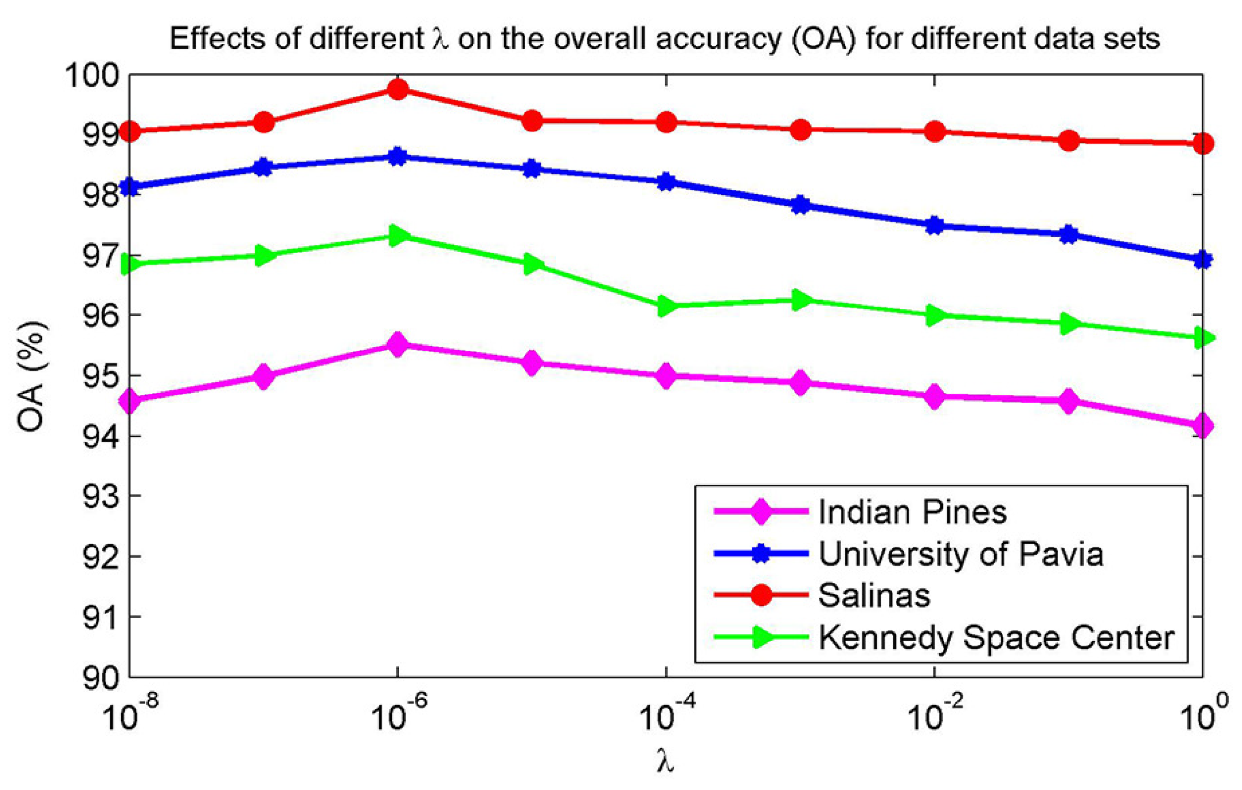
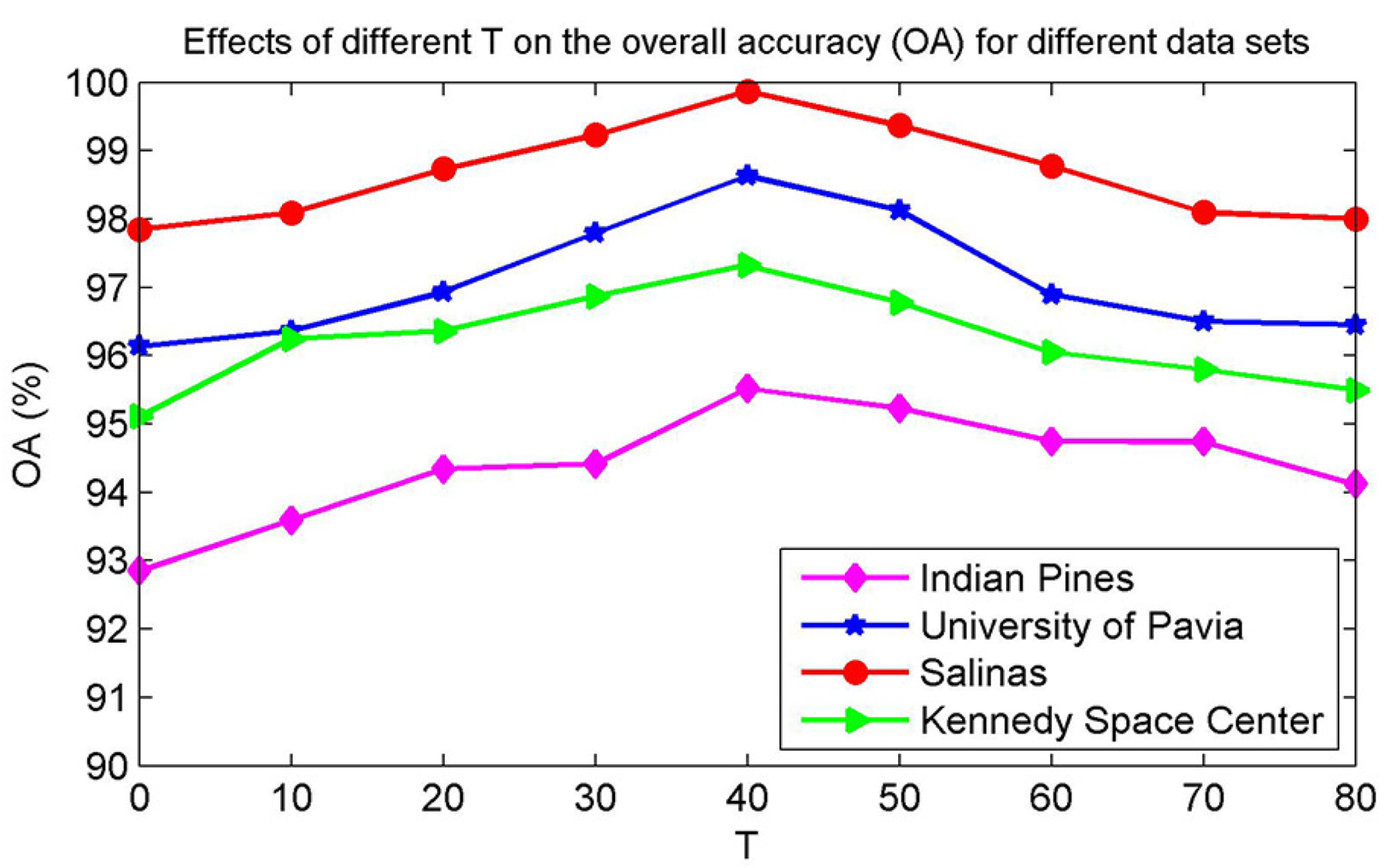
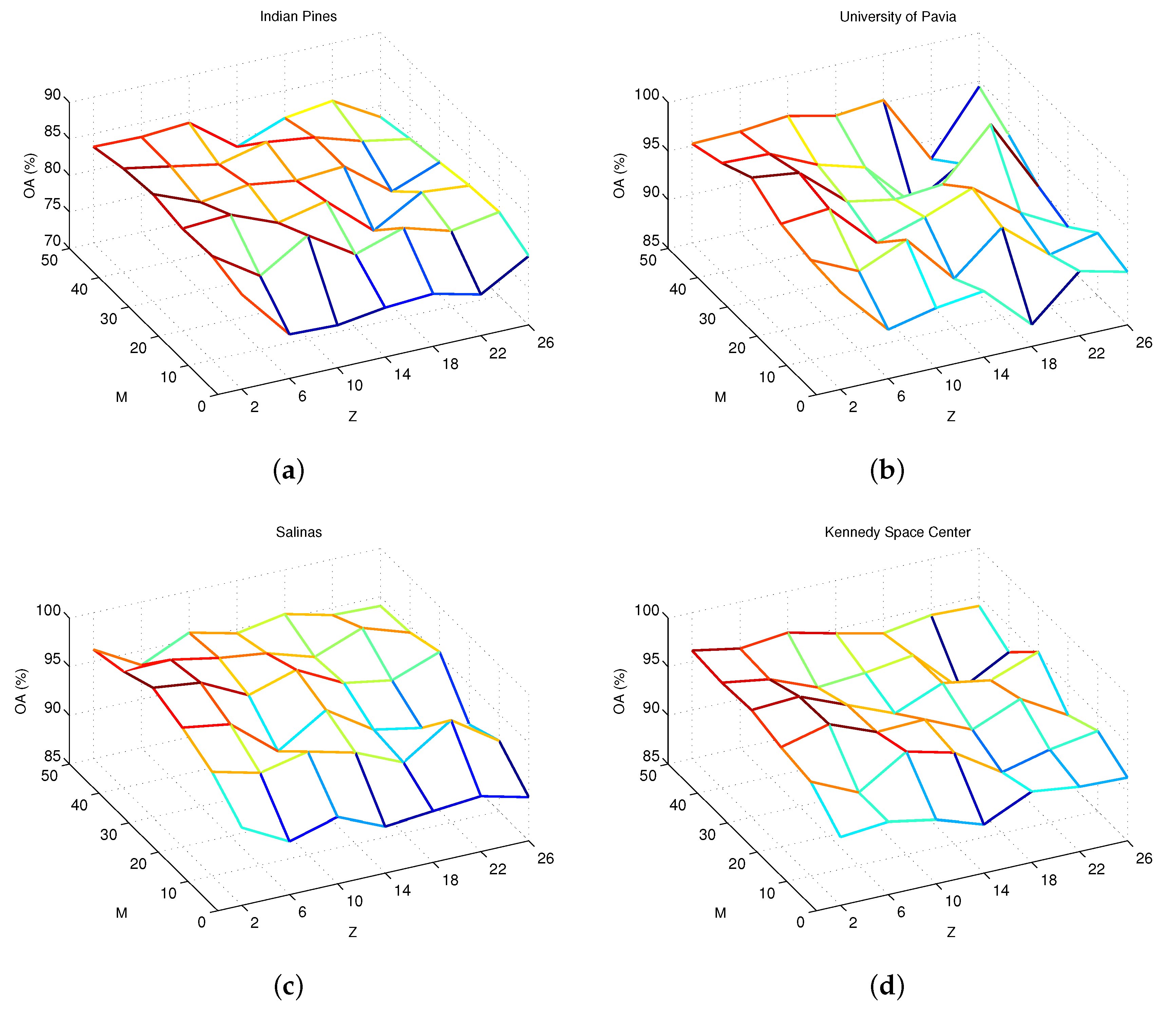
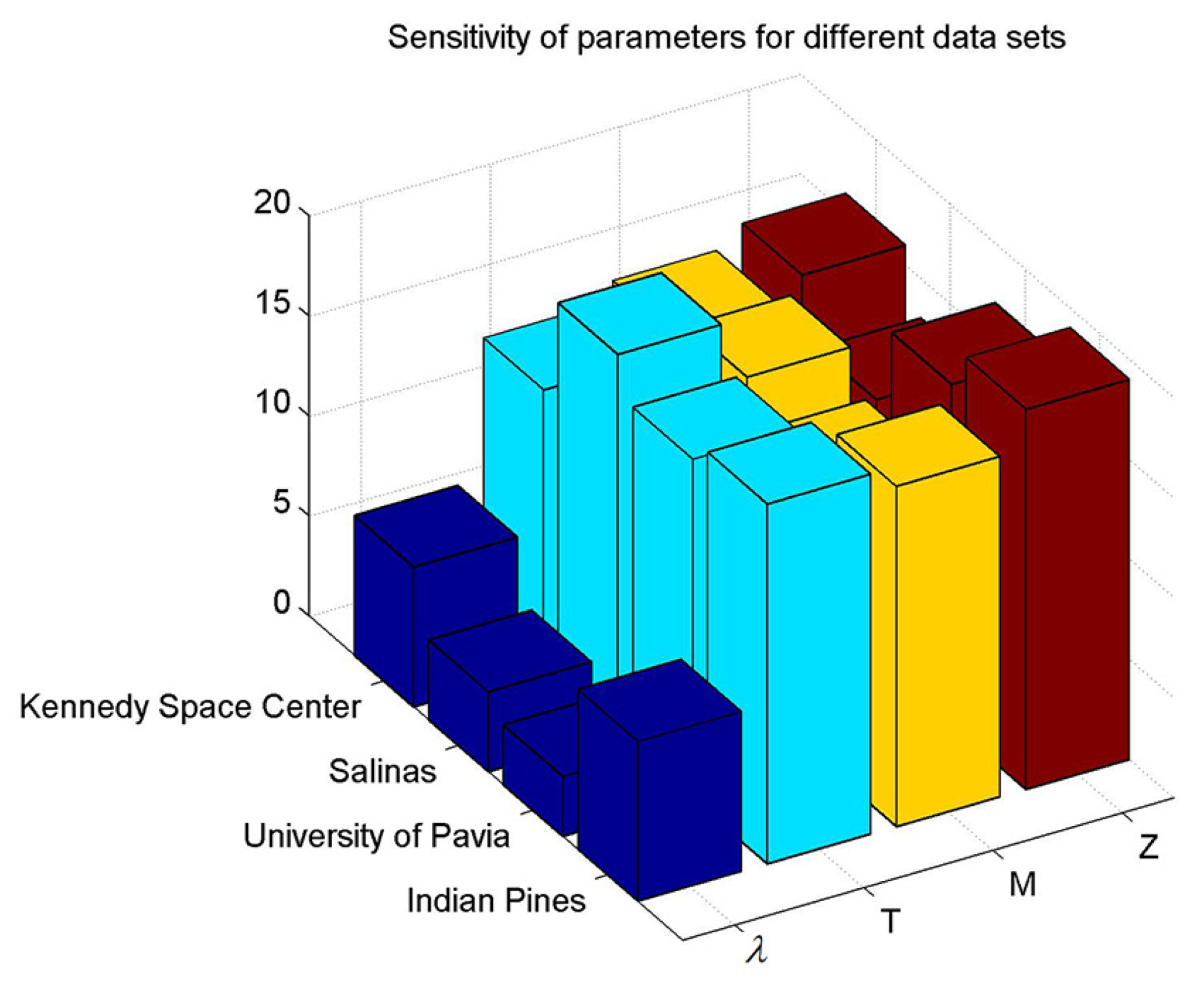
4.2. Parameter Analysis

(1) Analysis of the Influence of Parameter $\lambda$

For sparse representation, the regularization parameter $\lambda$ used in Equation (12) controls the relative importance between sparsity level and reconstruction error, leading to different classification accuracies. Figure 6 shows the effect of varying $\lambda$ on the classification accuracies for Indian Pines, University of Pavia, Salinas, and Kennedy Space Center data sets. In the experiment, the four different data sets are trained with 20 samples per class, respectively, and the remaining labeled samples are used for testing. The regularization parameter $\lambda$ for sparse representation is chosen between $\lambda =1\times {10}^{-8}$ and $\lambda =1$. In Figure 6, when $\lambda <1\times {10}^{-6}$, the overall accuracy (OA) shows an increasing trend on each data set. As $\lambda$ continues to increase, the overall trend of OA is decreasing. This is because more weight on sparsity level and less weight on approximation accuracy. Therefore, $\lambda =1\times {10}^{-6}$ is set as the optimal value in this paper.

(2) Analysis of the Influence of Parameter T

The parameter T is selected by using the five-fold cross-validation strategy and repeating the finetuning procedure. As described in Section 3.2, when the entropy of the sparse representation vector of a sample is small, the probability of that sample being a pure sample is large. As T increases, samples subsequently added will have a larger entropy, and these newly pseudo-labeled samples have a high probability of being mixed pixels. Thus, although the number of samples increases, the magnitude of the increase in the classification accuracy is small; consequently, it is important to choose a suitable T. In the experiment, the four different data sets are trained with 20 samples per class, respectively, and the remaining labeled samples are used for testing. Figure 7 shows the impact of different numbers of pseudo-labeled samples on the OA for the four data sets. The OA corresponding to different T values is the mean value of 30 random replicate experiments. As seen by observing Figure 7, for the different data sets, when T < 40, the OA tends to grow, although there is a downward trend in the interval related to the quality of the generated samples and the selected sample points. When T > 40, the OA shows a significant downward trend. In addition, when T = 40, the OAs are highest. Therefore, in this paper, we selected T = 40 as the default parameter value.

(3) Analysis of the Influences of Parameters M and Z

The parameters M and Z from Equation (8) are hyperparameters that require tuning. We evaluated the influences of the parameters M and Z by objective and visual analyses. In the experiment, the four different data sets are trained with 5, 20, 3, and 15 samples per class, respectively, and the remaining labeled samples are used for testing. Figure 8 shows the OA of the proposed SRSPL method of four different data sets. For the four data sets, as Figure 8 shows, as M and Z change, the OA exhibits large fluctuations. When M is less than 10, the accuracy of the proposed method is relatively low. This result indicates that, when M has few features, useful spectral information will be lost. Furthermore, the results show that the proposed method can achieve stable and high accuracy when the size of the subgroup is less than 8 because the IID method works for small channel images. In this paper, the default parameter settings M = 32 and Z = 4 were adopted for subsequent testing of the data sets.

(4) Sensitivity Analysis

The parameters involved in our proposed SRSPL method are mainly regularization parameter $\lambda$, the number of generated pseudo-labeled samples T, feature numbers M and different subgroup sizes Z. We have conducted an extensive experimental analysis of each parameter for the SRSPL method. The one-parameter-at-a-time (OAT) [47] approach is used for model parameter sensitivity analysis, that is, to ensure that other parameters remain unchanged when changing one parameter, and then to study the effect of one parameter on the model. Figure 9 shows the sensitivity of parameters $\lambda$, T, M and Z for four data sets. It can be seen that the sensitivity value of $\lambda$ on the four data sets is the smallest. However, parameters T, M, and Z show a higher sensitivity value on the four different data sets. Thus, it follows that the $\lambda$ has a slight effect on the SRSPL method and T, M, Z have a greater effect on the SRSPL method, which is highly sensitive and should be tuned.

4.3. Performance Evaluation

We applied the proposed SRSPL method and other methods to four hyperspectral images to evaluate the effectiveness of various hyperspectral image classification methods. We compared the proposed SRSPL method with several other classification methods, including the traditional SVM [48], three semi-supervised methods, e.g., extended random walker (ERW) [46], spatial-spectral label propagation based on SVM (SSLP-SVM) [49], the maximizer of the posterior marginal by loopy belief propagation (MPM-LBP) [50] and two deep learning methods, e.g., recurrent 2D convolutional neural network (R-2D-CNN) [51], cascaded recurrent neural network (CasRNN) [52]. IID [37] is used to extract the useful features and reduce noise in the proposed SRSPL method. Therefore, in order to verify the validity of the IID, an experiment that does not use the IID method is added (record as Without-IID). In this section, the effect of different feature extraction methods to the proposed method is also analyzed, e.g., principal component analysis (PCA) [53], image fusion, and recursive filtering (IFRF) [54] (record as With-PCA and With-IFRF, respectively). Here, the magnitude setting of the parameter T in the With-PCA and With-IFRF methods is the same as the SRSPL method. The SVM classifier was implemented from a library for LIBSVM and used a Gaussian kernel. The tests were performed using five-fold cross-validation.

The parameters for the ERW, SSLP-SVM, MPM-LBP, R-2D-CNN, CasRNN, PCA and IFRF methods were set to the default parameters reported in the corresponding papers. In this paper, three common metrics, namely: the OA, average accuracy (AA), and Kappa coefficient, were used to evaluate classifier performance. The classification results for each method are given as the average of 30 experiments to reduce the influence of sample randomness. The data on the left side of

Table 1. Classification performance of different methods performed on the Indian Pines data set with 5–25 training samples per class. Without-IID is the proposed method without the IID Step. With-PCA and With-IFRF denote the proposed method using different methods for feature extraction. (SVM, support vector machine; ERW, extended random walker; SSLP-SVM, spatial-spectral label propagation based on SVM; MPM-LBP, the maximizer of the posterior marginal by loopy belief propagation; R-2D-CNN, recurrent 2D convolutional neural network; CasRNN, cascaded recurrent neural network; SRSPL, sample pseudo-labeling method based on sparse representation. Three common metrics: overall accuracy (OA), average accuracy (AA), Kappa coefficient. The bold values indicate the greatest accuracy among the methods in each case.)

Method	Metric	Number of Training Samples per Class
		5	10	15	20	25
	OA	45.31 ± 5.19	57.58 ± 2.98	63.56 ± 2.61	66.92 ± 1.47	69.68 ± 0.97
SVM	AA	47.41 ± 3.71	55.19 ± 2.27	59.84 ± 2.21	62.13 ± 1.86	63.84 ± 0.91
	Kappa	39.21 ± 5.43	52.52 ± 3.17	59.11 ± 2.82	62.80 ± 1.56	65.82 ± 1.08
	OA	81.97 ± 5.93	86.89 ± 3.45	90.13 ± 3.47	92.64 ± 1.74	94.92 ± 1.70
Without-IID	AA	84.35 ± 6.40	89.07 ± 3.47	92.73 ± 1.23	95.63 ± 0.97	96.76 ± 0.95
	Kappa	80.91 ± 6.50	85.12 ± 3.77	89.42 ± 3.91	91.59 ± 1.99	94.20 ± 1.94
	OA	76.08 ± 3.60	82.62 ± 2.90	86.80 ± 2.13	90.90 ± 1.83	93.53 ± 1.55
With-PCA	AA	81.47 ± 4.20	80.47 ± 2.94	87.36 ± 3.51	91.02 ± 2.76	95.06 ± 0.79
	Kappa	73.03 ± 3.91	80.40 ± 3.20	85.30 ± 2.39	89.78 ± 2.07	92.61 ± 1.77
	OA	82.47 ± 2.30	88.62 ± 2.91	92.80 ± 2.13	94.90 ± 1.66	96.67 ± 1.21
With-IFRF	AA	89.68 ± 0.91	90.47 ± 0.94	93.36 ± 2.03	95.02 ± 2.63	97.83 ± 0.72
	Kappa	80.12 ± 2.56	89.40 ± 3.23	92.97 ± 1.96	93.78 ± 2.80	96.19 ± 1.39
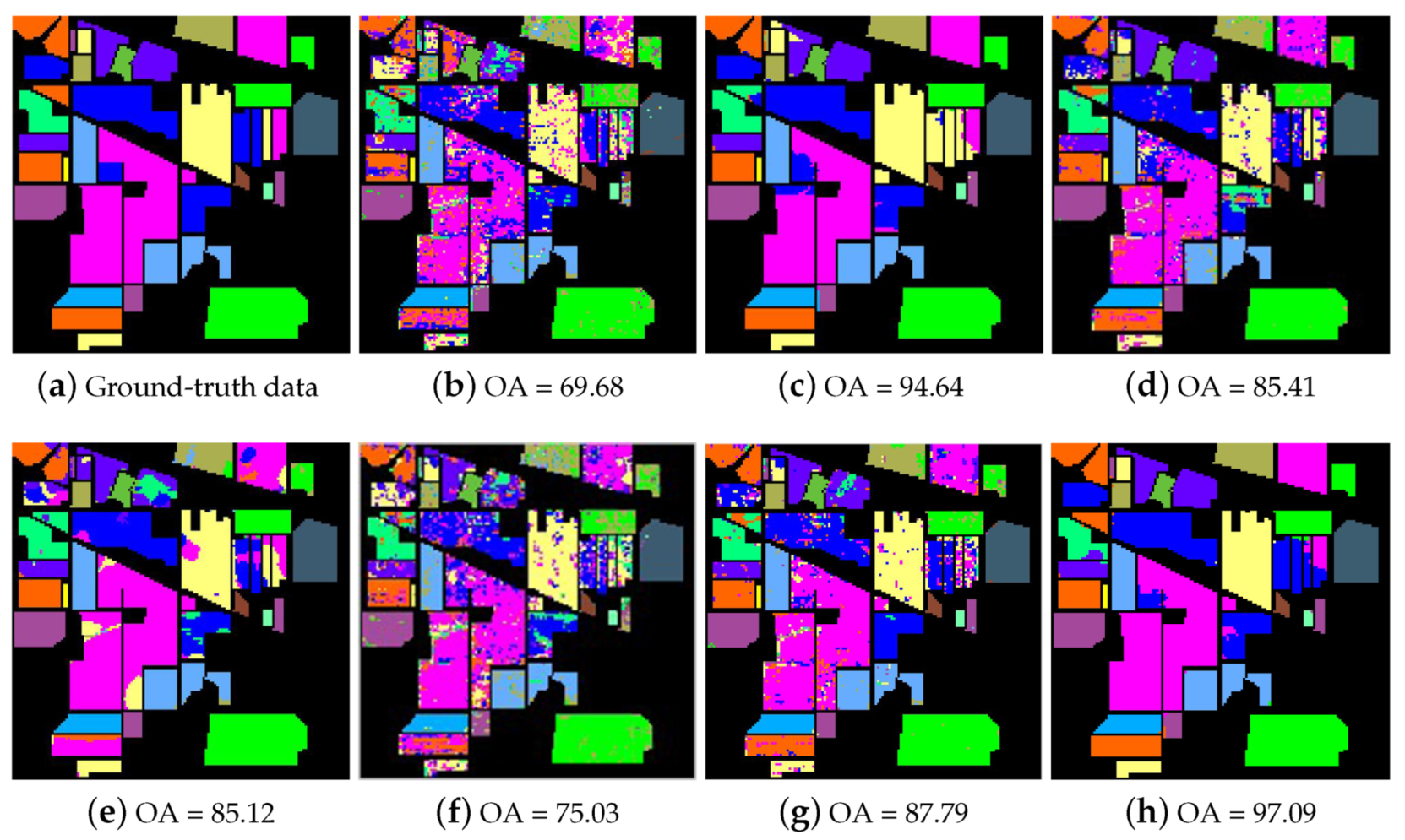
	OA	72.30 ± 4.38	84.87 ± 4.41	90.02 ± 1.30	92.94 ± 1.86	94.64 ± 1.17
ERW	AA	83.32 ± 2.41	91.48 ± 2.30	94.39 ± 0.94	96.18 ± 1.00	97.14 ± 0.62
	Kappa	68.96 ± 4.69	82.95 ± 4.86	88.69 ± 1.46	91.99 ± 2.10	93.91 ± 1.33
	OA	64.84 ± 1.43	76.05 ± 1.44	80.79 ± 0.73	82.13 ± 0.44	85.41 ± 0.26
SSLP-SVM	AA	65.96 ± 2.38	78.07 ± 0.98	82.08 ± 0.64	82.25 ± 0.68	86.87 ± 0.35
	Kappa	60.63 ± 1.49	73.17 ± 1.60	78.38 ± 0.80	79.90 ± 0.49	83.49 ± 0.29
	OA	59.36 ± 5.80	72.83 ± 3.99	78.15 ± 2.51	81.92 ± 2.17	85.12 ± 2.18
MPM-LBP	AA	72.10 ± 3.61	83.61 ± 1.27	87.34 ± 0.92	90.33 ± 1.63	91.82 ± 1.09
	Kappa	54.39 ± 6.31	69.50 ± 4.25	75.38 ± 2.75	79.61 ± 2.42	83.14 ± 2.42
	OA	51.63 ± 3.81	59.83 ± 3.79	64.15 ± 2.18	70.92 ± 1.07	75.03 ± 1.18
R-2D-CNN	AA	52.01 ± 3.16	58.61 ± 2.72	65.43 ± 1.21	69.33 ± 1.36	76.82 ± 1.39
	Kappa	50.93 ± 3.13	60.50 ± 2.52	63.82 ± 1.57	71.61 ± 1.24	74.19 ± 1.43
	OA	60.57 ± 4.51	70.25 ± 2.18	75.22 ± 2.23	81.43 ± 1.69	87.79 ± 1.50
CasRNN	AA	58.44 ± 3.12	72.86 ± 1.87	76.59 ± 1.74	83.66 ± 1.87	88.94 ± 1.21
	Kappa	60.92 ± 3.58	69.34 ± 2.74	74.54 ± 2.05	80.49 ± 1.72	86.62 ± 1.74
	OA	84.73 ± 1.23	90.90 ± 1.25	93.88 ± 0.67	95.52 ± 0.39	97.09 ± 0.21
SRSPL	AA	88.86 ± 1.51	93.97 ± 0.95	96.27 ± 0.58	97.04 ± 0.57	97.96 ± 0.39
	Kappa	81.79 ± 1.45	89.64 ± 1.05	93.02 ± 0.72	94.88 ± 0.45	96.66 ± 0.27

,

Table 2. Classification accuracies (University of Pavia) in percentages for the tested methods when 20 training samples per class are provided. (The bold values indicate the greatest accuracy among the methods in each case.)

Class	Training	Test	SVM	Without-IID	Different Feature Extraction Methods		Different Semi-Supervised Methods			Deep Learning Methods		SRSPL
					With-PCA	With-IFRF	ERW	SSLP-SVM	MPM-LBP	R-2D-CNN	CasRNN
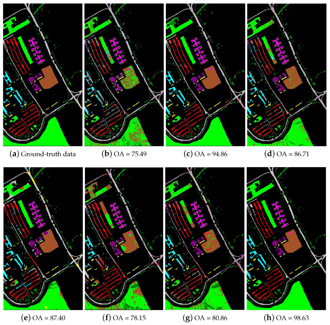
Asphalt	20	6611	92.99 ± 2.27	90.92 ± 2.21	70.23 ± 6.45	99.84 ± 0.03	86.36 ± 6.78	96.22 ± 0.64	90.39 ± 8.38	79.34 ± 5.38	83.52 ± 6.33	98.93 ± 1.33
Meadows	20	18,629	90.78 ± 2.36	99.99 ± 0.58	80.84 ± 4.31	90.03 ± 3.61	98.32 ± 2.67	97.65 ± 0.20	92.95 ± 11.81	79.96 ± 3.61	71.37 ± 5.81	99.48 ± 0.57
Gravel	20	2079	55.61 ± 6.89	99.86 ± 0.07	98.98 ± 0.74	98.97 ± 0.03	96.34 ± 5.82	71.05 ± 1.69	85.25 ± 8.21	78.88 ± 6.12	64.51 ± 10.21	99.95 ± 0.03
Trees	20	3044	67.48 ± 10.20	85.81 ± 2.07	89.01 ± 5.77	90.70 ± 3.45	78.92 ± 4.07	81.88 ± 4.50	89.48 ± 5.91	73.91 ± 4.48	85.43 ± 3.42	91.86 ± 1.66
Metal Sheets	20	1325	94.27 ± 3.49	100.00 ± 0.00	99.31 ± 0.16	99.77 ± 0.02	99.66 ± 0.27	96.95 ± 1.91	98.56 ± 0.66	98.25 ± 0.20	98.55 ± 0.47	99.62 ± 0.20
Bare Soil	20	5009	49.36 ± 7.80	92.25 ± 3.42	85.18 ± 7.13	98.42 ± 2.50	97.04 ± 3.62	66.64 ± 4.67	87.25 ± 10.38	80.94 ± 4.51	89.08 ± 5.25	98.49 ± 0.08
Bitumen	20	1310	53.58 ± 6.35	100.00 ± 0.00	99.19 ± 0.53	95.53 ± 1.85	99.42 ± 0.33	60.77 ± 3.59	97.94 ± 1.66	78.49 ± 2.92	91.13 ± 2.62	99.95 ± 0.09
Bricks	20	3662	76.30 ± 5.67	98.00 ± 1.83	98.14 ± 1.00	97.71 ± 2.85	97.34 ± 2.13	87.75 ± 1.46	88.32 ± 5.45	83.81 ± 2.45	93.54 ± 3.41	99.84 ± 3.07
Shadows	20	927	99.88 ± 0.09	98.05 ± 0.09	94.45 ± 1.48	98.88 ± 0.15	99.89 ± 0.09	99.95 ± 0.13	98.78 ± 1.58	94.27 ± 0.30	94.72 ± 1.78	99.03 ± 0.06
OA			75.49 ± 3.45	96.62 ± 1.35	83.49 ± 1.86	96.76 ± 1.15	94.86 ± 1.33	86.71 ± 1.44	87.40 ± 4.70	78.15 ± 1.47	80.86 ± 3.74	98.63 ± 0.31
AA			76.06 ± 1.98	96.42 ± 2.98	88.61 ± 2.56	96.54 ± 2.74	95.02 ± 3.25	88.55 ± 2.15	88.75 ± 2.05	79.19 ± 1.35	84.29 ± 4.53	98.34 ± 0.13
Kappa			69.06 ± 3.94	95.52 ± 1.72	79.88 ± 2.21	95.18 ± 3.73	93.19 ± 1.73	82.92 ± 1.75	87.62 ± 5.48	77.34 ± 1.81	77.93 ± 3.18	98.18 ± 0.41

and

Table 3. Classification accuracies (University of Pavia) in percentages for the tested methods when 20 training samples per class are provided. (The bold values indicate the greatest accuracy among the methods in each case.)

Class	Training	Test	SVM	Without-IID	Different Feature Extraction Methods		Different Semi-Supervised Methods			Deep Learning Methods		SRSPL
					With-PCA	With-IFRF	ERW	SSLP-SVM	MPM-LBP	R-2D-CNN	CasRNN
Weeds 1	3	2006	86.74 ± 12.68	96.74 ± 12.68	100.00 ± 0.00	100.00 ± 0.00	100.00 ± 0.00	99.87 ± 0.15	98.82 ± 0.80	88.83 ± 1.85	90.12 ± 1.28	100.00 ± 0.00
Weeds 2	3	3723	99.08 ± 0.89	99.08 ± 0.89	100.00 ± 0.00	99.34 ± 0.04	99.95 ± 0.03	98.75 ± 0.24	99.40 ± 0.67	99.46 ± 0.37	99.20 ± 0.69	99.96 ± 0.06
Fallow	3	1973	77.08 ± 16.42	98.08 ± 1.42	100.00 ± 0.00	100.00 ± 0.00	100.00 ± 0.00	84.21 ± 2.16	90.98 ± 12.66	79.49 ± 2.66	81.88 ± 3.76	100.00 ± 0.00
Fallow_P	3	1391	96.94 ± 1.23	84.94 ± 1.23	96.81 ± 3.16	85.28 ± 6.84	86.28 ± 7.64	97.64 ± 0.12	99.47 ± 0.30	96.13 ± 0.46	97.48 ± 0.47	94.64 ± 2.84
Fallow_S	3	2675	90.08 ± 8.26	97.08 ± 1.26	97.36 ± 2.97	98.41 ± 0.25	99.41 ± 0.27	96.86 ± 3.22	97.94 ± 1.53	90.07 ± 1.35	92.97 ± 1.73	97.38 ± 6.17
Stubble	3	3956	99.11 ± 4.76	98.11 ± 1.76	98.00 ± 2.01	97.34 ± 1.58	97.72 ± 4.58	99.87 ± 0.25	97.75 ± 3.28	97.81 ± 1.78	97.89 ± 0.38	99.92 ± 0.06
Celery	3	3576	93.79 ± 4.17	98.79 ± 1.17	100.00 ± 0.00	90.20 ± 4.77	72.20 ± 24.77	98.95 ± 0.41	99.06 ± 0.84	94.91 ± 2.43	96.56 ± 1.64	99.35 ± 0.18
Grapes	3	11268	64.24 ± 7.87	94.24 ± 2.87	93.12 ± 2.18	99.15 ± 0.42	99.17 ± 0.92	72.05 ± 3.23	72.48 ± 18.65	70.84 ± 6.55	73.45 ± 7.67	99.70 ± 2.56
Soil	3	6200	96.20 ± 3.03	96.20 ± 2.03	98.38 ± 1.48	100.00 ± 0.00	100.00 ± 0.00	99.37 ± 0.17	99.21 ± 0.60	96.18 ± 1.06	97.41 ± 0.78	100.00 ± 0.00
Corn	3	3275	72.58 ± 19.06	97.58 ± 1.06	91.57 ± 6.35	97.21 ± 7.15	95.36 ± 7.15	89.21 ± 3.90	83.91 ± 10.82	75.06 ± 10.28	78.04 ± 9.12	97.36 ± 9.51
Lettuce_4	3	1065	74.66 ± 19.37	96.66 ± 2.37	80.51 ± 6.47	98.76 ± 2.23	100.00 ± 0.00	83.41 ± 4.40	92.94 ± 4.87	77.27 ± 8.78	80.64 ± 6.76	99.98 ± 0.06
Lettuce_5	3	1924	81.48 ± 10.07	98.48 ± 0.07	83.16 ± 12.54	99.60 ± 1.83	100.00 ± 0.00	92.60 ± 5.67	99.36 ± 1.97	83.55 ± 7.75	85.61 ± 5.67	100.00 ± 0.00
Lettuce_6	3	913	78.58 ± 13.93	98.58 ± 0.93	98.31 ± 2.74	98.74 ± 0.47	97.88 ± 0.47	95.24 ± 0.66	97.17 ± 3.24	80.20 ± 6.24	82.80 ± 4.41	98.47 ± 0.27
Lettuce_7	3	1067	83.59 ± 19.14	93.59 ± 2.14	97.24 ± 2.59	95.33 ± 2.21	95.35 ± 2.36	92.14 ± 4.74	94.76 ± 2.63	85.73 ± 7.36	88.78 ± 5.37	96.26 ± 0.68
Vinyard_U	3	7265	45.43 ± 6.21	97.43 ± 2.21	88.51 ± 8.64	99.37 ± 0.17	99.18 ± 0.05	58.67 ± 7.83	70.93 ± 25.10	71.81 ± 10.01	75.93 ± 9.70	98.92 ± 0.13
Vinyard_T	3	1804	83.43 ± 18.80	99.43 ± 0.80	100.00 ± 0.00	99.48 ± 0.89	100.00 ± 0.00	71.12 ± 4.44	76.88 ± 11.35	86.12 ± 6.35	89.06 ± 4.35	99.68 ± 0.79
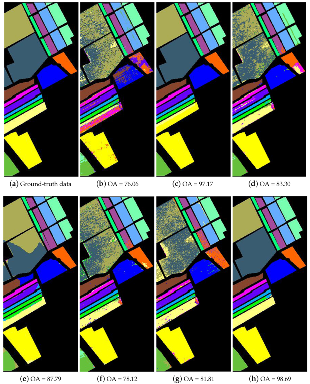
OA			76.06 ± 2.97	95.88 ± 3.63	86.06 ± 2.97	97.65 ± 1.36	97.17 ± 2.23	83.30 ± 1.58	87.79 ± 3.26	78.12 ± 2.42	81.81 ± 3.89	98.69 ± 1.22
AA			82.69 ± 2.46	96.76 ± 2.64	90.69 ± 2.46	97.78 ± 1.69	96.62 ± 2.69	88.12 ± 0.78	92.57 ± 2.07	77.45 ± 2.04	82.34 ± 2.10	98.01 ± 1.44
Kappa			73.52 ± 3.22	94.59 ± 3.97	85.52 ± 3.22	98.00 ± 1.45	96.84 ± 2.49	81.46 ± 1.72	86.41 ± 3.63	79.47 ± 2.31	80.87 ± 3.38	98.54 ± 1.37

represent the mean values, while those on the right represent the standard deviations.

The experiment was first performed on the Indian Pines date set. As shown in Table 1, the training samples were randomly selected and accounted for 5, 10, 15, 20, and 25 per class of the reference data. Note that, as the number of training samples increases, the classification accuracy grows steadily. The proposed SRSPL method always outperforms the other methods, such as ERW, SSLP-SVM, and MPM-LBP, in terms of the highest overall classification accuracies; this method obtained the highest accuracies in all cases (84.73%, 90.90%, 93.88%, 95.52% and 97.09%, respectively). Compared with the two deep learning methods R-2D-CNN and CasRNN, the SRSPL method can achieve higher accuracy in the case of small samples. Compared with the three methods of Without-IID, With-PCA, and With-IFRF, Table 1 shows that the proposed SRSPL method obtains higher accuracies, which indicates that feature extraction using the IID method is effective.

Figure 10 shows the classification maps obtained for the Indian Pines data set with the five methods when using 25 training samples from each class. As shown in Figure 10c–g, the proposed SRSPL method performs better than the other classification methods (i.e., ERW, SSLP-SVM, MPM-LBP, R-2D-CNN, and CasRNN) when fewer training samples are provided. For example, the classification maps of the SVM, SSLP-SVM, MPM-LBP, R-2D-CNN, and CasRNN methods include more noise, and the ERW method does not perform as well as the SRSPL method does on certain classes.

Table 2 shows the experimental results using the University of Pavia data set when the number of training samples per class is 20. As Table 2 shows, the nine compared methods achieve various performance characteristics when only 20 training samples per class are provided. The proposed SRSPL method not only outperforms the R-2D-CNN and CasRNN methods, which are the state-of-the-art methods based on deep learning in the hyperspectral image classification, but also outperforms the other compared methods by 2–20%. Notably, on classes such as “Asphalt” and “Trees”, the proposed SRSPL method performs much better than does the ERW method-by 12.57% and 12.94%, respectively. In the feature extraction experiment, the OA of the proposed SRSPL method outperforms the Without-IID, With-PCA, and With-IFRF methods by 2.01%, 15.14%, and 1.87%, respectively. Figure 11 shows the classification maps obtained for the University of Pavia data set with the different methods when using 20 training samples from each class. As Figure 11 shows, the SRSPL method is superior to other semi-supervised and deep learning methods in visual appearance, which shows its effectiveness.

The third experiment was conducted on the Salinas data set. In Table 3, three training samples per class were randomly selected for training, and the rest were used for testing. Given the limited samples, the experiment is quite challenging. The corresponding quantitative values of the classification results are tabulated in Table 3. As shown, although only limited training samples were provided, some of the methods achieved high OA and Kappa scores. In fact, some of the methods achieved 100% classification accuracy on several classes. This is because the Salinas image includes many large uniform regions that make classification simpler. Compared with the other methods, the proposed SRSPL method greatly improves the classification accuracy when training samples are extremely limited. Because the R-2D-CNN and CasRNN methods require a large number of samples for training, when there are small training samples, it is easy to produce overfitting and thus lead to poor classification results. As seen from Figure 12, the proposed SRSPL method can classify most of the features correctly, which reflects the effectiveness of the method.

The fourth experiment was performed on the Kennedy Space Center data set. In the experiment, the proposed SRSPL method was compared with the SVM method and three other semi-supervised methods, e.g., ERW, SSLP-SVM, MPM-LBP, and two different deep learning methods, e.g., R-2D-CNN, CasRNN. Figure 13 shows the changes in OA and Kappa coefficient as the number of training samples per class increases from 3 to 15. Compared with the deep learning-based classification methods R-2D-CNN and CasRNN, the proposed SRSPL method shows great advantages. As shown in Figure 13, the SRSPL method achieves the highest accuracy among the tested methods.

Finally, we evaluated the computational times of the three different semi-supervised methods (i.e., MPM-LBP, SSLP-SVM, and SRSPL) on the four different data sets using 20 samples per class using MATLAB on a computer with 3.6 GHz CPU and 8-GB memory. Because the semi-supervised method proposed in this paper does not involve a single training process, its computational cost is greatly improved.

Table 4. Execution times of three semi-supervised methods of four data sets. (The bold values indicate the minimum computational times among the methods in each data set.)

Data Sets	Computational Times (s)
	MPM-LBP	SSLP-SVM	SRSPL
Indian Pines	197.78	479.51	124.31
University of Pavia	604.35	164.09	240.14
Salinas	339.03	1592.75	202.14
Kennedy Space Center	939.519	122.20	72.32

shows that the proposed SRSPL method requires less time to process the Indian Pines, Salinas, and Kennedy Space Center data sets than do the other tested methods.

5. Discussion

In hyperspectral image classification, it is difficult and expensive to obtain enough labeled samples for model training. Considering the strong spectral correlation between labeled and unlabeled samples in the image, we proposed a novel sparse representation-based sample pseudo-labeling method (SRSPL). The pseudo-labeled samples generated by this method can be used to augment the training set, thereby solving the problem of poor classification performance under the condition of small samples.

Compared with other pseudo-labeled sample generation method (such as SSLP-SVM), the proposed SRSPL method is more reliable in generating pseudo-labeled samples. The SSLP-SVM method only adds a small number of pseudo-labeled samples near the labeled samples, and the added samples may be mixed samples. The proposed SRSPL method considers the relationship between sample purity and information entropy, that is, the purer the sample’s spectrum, the lower the information entropy of the sparse representation coefficient, and vice versa. Specifically, the spectral characteristics of a pure sample can be linearly represented using a single class of atoms in an overcomplete dictionary, so its coefficient vector will have smaller entropy. In our method, pure samples with smaller entropy are used to expand the initial training sample set, which can greatly improve classifier performance.

In the case of small samples, compared with other classifiers (such as SVM, ERW, and MPM-LBP), the SRSPL method produces a good classification map for each hyperspectral data set visually, as shown in Figure 9, Figure 10 and Figure 11. This is because the hyperspectral image is first processed using the intrinsic image decomposition technology, which helps reduce errors in subsequent sparse representations, and the pseudo-label samples generated by the SRSPL method can help optimize the classification model. In addition, compared with deep-learning-based classifiers (such as R-2D-CNN and CasRNN), the proposed SRSPL method performs better for a limited number of samples because, in such cases, these two methods are more likely to overfit the training samples, resulting in poor classification results. Thus, the proposed SRSPL method shows better classification results than other comparative methods.

6. Conclusions

In this paper, we proposed a novel sample pseudo-labeling method based on sparse representation that addresses the problem of limited samples. The previously proposed semi-supervised methods for generating pseudo-labeled samples typically select some samples and assign them a pseudo-label based on spectral information correlations or local neighborhood information. However, due to the presence of mixed pixels, the selected samples are not necessarily representative. To find the purest samples, we designed a sparse representation-based pseudo-labeling method that utilizes the coefficient vector of sparse representation and draws on the definition and idea of entropy from information theory. Overall, the proposed SRSPL method provides a new option for semi-supervised learning, which is the first contribution of the paper. Moreover, the proposed SRSPL method also solves the problem of uneven sample distribution through sparse representation based on spectral features, which is beneficial for subsequent classification. In addition, by comparing the standard deviations of OA, AA, and Kappa of 30 random replicate experiments with other state-of-the-art classification methods, we found that the proposed SRSPL method had higher robustness and stability. This is the second contribution of the paper. The experimental results on four real-world hyperspectral images show that the proposed SRSPL method is superior to other state-of-the-art classification methods from the perspectives of both quantitative indicators and classification maps.

References

- Kang, X.; Li, C.; Li, S.; Lin, H. Classification of hyperspectral images by Gabor filtering based deep network. IEEE J. Sel. Top. Appl. Earth Obs. Remote Sens. 2017, 11, 1166–1178. [Google Scholar] [CrossRef]
- Pontius, J.; Martin, M.; Plourde, L.; Hallett, R. Ash decline assessment in emerald ash borer-infested regions: A test of tree-level, hyperspectral technologies. Remote Sens. Environ. 2008, 112, 2665–2676. [Google Scholar] [CrossRef]
- Imani, M. Manifold structure preservative for hyperspectral target detection. Adv. Space Res. 2018, 61, 2510–2520. [Google Scholar] [CrossRef]
- Cao, X.; Zhou, F.; Xu, L.; Meng, D.; Xu, Z.; Paisley, J. Hyperspectral image classification with Markov random fields and a convolutional neural network. IEEE Trans. Image Process. 2018, 27, 2354–2367. [Google Scholar] [CrossRef]
- Sharma, S.; Buddhiraju, K.M. Spatial–spectral ant colony optimization for hyperspectral image classification. Int. J. Remote Sens. 2018, 39, 2702–2717. [Google Scholar] [CrossRef]
- Hughes, G. On the mean accuracy of statistical pattern recognizers. IEEE Trans. Inf. Theory 1968, 14, 55–63. [Google Scholar] [CrossRef]
- Xia, J.; Du, P.; He, X.; Chanussot, J. Hyperspectral remote sensing image classification based on rotation forest. IEEE Geosci. Remote Sens. Lett. 2013, 11, 239–243. [Google Scholar] [CrossRef]
- Mohanty, R.; Happy, S.; Routray, A. Spatial–Spectral Regularized Local Scaling Cut for Dimensionality Reduction in Hyperspectral Image Classification. IEEE Geosci. Remote Sens. Lett. 2018, 16, 932–936. [Google Scholar] [CrossRef]
- Shamsolmoali, P.; Zareapoor, M.; Yang, J. Convolutional neural network in network (CNNiN): Hyperspectral image classification and dimensionality reduction. IET Image Process. 2018, 13, 246–253. [Google Scholar] [CrossRef]
- Fang, B.; Li, Y.; Zhang, H.; Chan, J. Semi-supervised deep learning classification for hyperspectral image based on dual-strategy sample selection. Remote Sens. 2018, 10, 574. [Google Scholar] [CrossRef]
- Cui, B.; Xie, X.; Hao, S.; Cui, J.; Lu, Y. Semi-supervised classification of hyperspectral images based on extended label propagation and rolling guidance filtering. Remote Sens. 2018, 10, 515. [Google Scholar] [CrossRef]
- Liu, B.; Yu, X.; Zhang, P.; Yu, A.; Fu, Q.; Wei, X. Supervised deep feature extraction for hyperspectral image classification. IEEE Trans. Geosci. Remote Sens. 2017, 56, 1909–1921. [Google Scholar] [CrossRef]
- He, N.; Paoletti, M.E.; Haut, J.M.; Fang, L.; Li, S.; Plaza, A.; Plaza, J. Feature extraction with multiscale covariance maps for hyperspectral image classification. IEEE Trans. Geosci. Remote Sens. 2018, 57, 755–769. [Google Scholar] [CrossRef]
- Medjahed, S.A.; Ouali, M. Band selection based on optimization approach for hyperspectral image classification. Egyptian J. Remote Sens. Space Sci. 2018, 21, 413–418. [Google Scholar] [CrossRef]
- Cui, B.; Xie, X.; Ma, X.; Ren, G.; Ma, Y. Superpixel-based extended random walker for hyperspectral image classification. IEEE Trans. Geosci. Remote Sens. 2018, 56, 3233–3243. [Google Scholar] [CrossRef]
- Jamshidpour, N.; Homayouni, S.; Safari, A. Graph-based semi-supervised hyperspectral image classification using spatial information. In Proceedings of the Workshop on Hyperspectral Image and Signal Processing: Evolution in Remote Sensing (WHISPERS), Los Angeles, LA, USA, 21–24 August 2016; pp. 1–4. [Google Scholar]
- Haut, J.M.; Paoletti, M.E.; Plaza, J.; Li, J.; Plaza, A. Active learning with convolutional neural networks for hyperspectral image classification using a new bayesian approach. IEEE Trans. Geosci. Remote Sens. 2018, 56, 6440–6461. [Google Scholar] [CrossRef]
- Wang, Z.; Du, B.; Zhang, L.; Zhang, L.; Jia, X. A novel semisupervised active-learning algorithm for hyperspectral image classification. IEEE Trans. Geosci. Remote Sens. 2017, 55, 3071–3083. [Google Scholar] [CrossRef]
- Li, J.; Xi, B.; Li, Y.; Du, Q.; Wang, K. Hyperspectral classification based on texture feature enhancement and deep belief networks. Remote Sens. 2018, 10, 396. [Google Scholar] [CrossRef]
- Zhou, S.; Chen, Q.; Wang, X. Fuzzy deep belief networks for semi-supervised sentiment classification. Neurocomputing 2014, 131, 312–322. [Google Scholar] [CrossRef]
- Sun, B.; Kang, X.; Li, S.; Benediktsson, J.A. Random-walker-based collaborative learning for hyperspectral image classification. IEEE Trans. Geosci. Remote Sens. 2016, 55, 212–222. [Google Scholar] [CrossRef]
- Imani, M.; Ghassemian, H. Adaptive expansion of training samples for improving hyperspectral image classification performance. In Proceedings of the Iranian Conference on Electrical Engineering (ICEE), Mashhad, Iran, 14–16 May 2013; pp. 1–6. [Google Scholar]
- Wu, H.; Prasad, S. Semi-supervised deep learning using pseudo labels for hyperspectral image classification. IEEE Trans. Image Process. 2017, 27, 1259–1270. [Google Scholar] [CrossRef] [PubMed]
- Ma, D.; Tang, P.; Zhao, L. SiftingGAN: Generating and Sifting Labeled Samples to Improve the Remote Sensing Image Scene Classification Baseline In Vitro. IEEE Geosci. Remote Sens. Lett. 2019, 16, 1046–1050. [Google Scholar] [CrossRef]
- Prasad, S.; Labate, D.; Cui, M.; Zhang, Y. Morphologically decoupled structured sparsity for rotation-invariant hyperspectral image analysis. IEEE Trans. Geosci. Remote Sens. 2017, 55, 4355–4366. [Google Scholar] [CrossRef]
- Prasad, S.; Labate, D.; Cui, M.; Zhang, Y. Rotation invariance through structured sparsity for robust hyperspectral image classification. In Proceedings of the International Conference on Acoustics, Speech and Signal Processing (ICASSP), New Orleans, LA, USA, 5–9 March 2017; pp. 6205–6209. [Google Scholar]
- Li, J.; Zhang, H.; Zhang, L. Efficient superpixel-level multitask joint sparse representation for hyperspectral image classification. IEEE Trans. Geosci. Remote Sens. 2015, 53, 5338–5351. [Google Scholar]
- Tu, B.; Zhang, X.; Kang, X.; Zhang, G.; Wang, J.; Wu, J. Hyperspectral image classification via fusing correlation coefficient and joint sparse representation. IEEE Geosci. Remote Sens. Lett. 2018, 15, 340–344. [Google Scholar] [CrossRef]
- Chen, Y.; Nasrabadi, N.M.; Tran, T.D. Hyperspectral image classification via kernel sparse representation. IEEE Trans. Geosci. Remote Sens. 2012, 51, 217–231. [Google Scholar] [CrossRef]
- Gan, L.; Xia, J.; Du, P.; Chanussot, J. Multiple feature kernel sparse representation classifier for hyperspectral imagery. IEEE Trans. Geosci. Remote Sens. 2018, 56, 5343–5356. [Google Scholar] [CrossRef]
- Liu, J.; Xiao, Z.; Chen, Y.; Yang, J. Spatial-spectral graph regularized kernel sparse representation for hyperspectral image classification. ISPRS Int. J. Geo-Inf. 2017, 6, 258. [Google Scholar] [CrossRef]
- Fang, L.; Wang, C.; Li, S.; Benediktsson, J.A. Hyperspectral image classification via multiple-feature-based adaptive sparse representation. IEEE Trans. Instrum. Meas. 2017, 66, 1646–1657. [Google Scholar] [CrossRef]
- Tong, F.; Tong, H.; Jiang, J.; Zhang, Y. Multiscale union regions adaptive sparse representation for hyperspectral image classification. Remote Sens. 2017, 9, 872. [Google Scholar] [CrossRef]
- Pan, B.; Shi, Z.; Xu, X. Multiobjective-based sparse representation classifier for hyperspectral imagery using limited samples. IEEE Trans. Geosci. Remote Sens. 2018, 57, 239–249. [Google Scholar] [CrossRef]
- Jian, M.; Jung, C. Class-discriminative kernel sparse representation-based classification using multi-objective optimization. IEEE Trans. Signal Process. 2013, 61, 4416–4427. [Google Scholar] [CrossRef]
- Sun, X.; Yang, L.; Zhang, B.; Gao, L.; Gao, J. An endmember extraction method based on artificial bee colony algorithms for hyperspectral remote sensing images. Remote Sens. 2015, 7, 16363–16383. [Google Scholar] [CrossRef]
- Kang, X.; Li, S.; Fang, L.; Benediktsson, J.A. Intrinsic image decomposition for feature extraction of hyperspectral images. IEEE Trans. Geosci. Remote Sens. 2014, 53, 2241–2253. [Google Scholar] [CrossRef]
- Tappen, M.F.; Freeman, W.T.; Adelson, E.H. Recovering intrinsic images from a single image. In Advances in Neural Information Processing Systems; Massachusetts Institute of Technology Press: Cambridge, MA, USA, 2003; pp. 1367–1374. [Google Scholar]
- Yacoob, Y.; Davis, L.S. Segmentation using appearance of mesostructure roughness. Int. J. Comput. Vis. 2009, 83, 248–273. [Google Scholar] [CrossRef]
- Shen, J.; Yang, X.; Li, X.; Jia, Y. Intrinsic image decomposition using optimization and user scribbles. IEEE Trans. Cybern. 2013, 43, 425–436. [Google Scholar] [CrossRef]
- Shen, J.; Yang, X.; Jia, Y.; Li, X. Intrinsic images using optimization. In Proceedings of the Conference on Computer Vision and Pattern Recognition (CVPR), Providence, RI, USA, 20–25 June 2011; pp. 3481–3487. [Google Scholar]
- Wright, J.; Yang, A.Y.; Ganesh, A.; Sastry, S.S.; Ma, Y. Robust face recognition via sparse representation. IEEE Trans. Pattern Anal. Mach. Intell. 2008, 31, 210–227. [Google Scholar] [CrossRef]
- Chen, Y.; Nasrabadi, N.M.; Tran, T.D. Hyperspectral image classification using dictionary-based sparse representation. IEEE Trans. Geosci. Remote Sens. 2011, 49, 3973–3985. [Google Scholar] [CrossRef]
- Tibshirani, R. Regression shrinkage and selection via the lasso: A retrospective. J. R. Stat. Soc. Ser. (Stat. Methodol.) 2011, 73, 273–282. [Google Scholar] [CrossRef]
- Nitanda, A. Stochastic proximal gradient descent with acceleration techniques. In Advances in Neural Information Processing Systems; Massachusetts Institute of Technology Press: Cambridge, MA, USA, 2014; pp. 1574–1582. [Google Scholar]
- Kang, X.; Li, S.; Fang, L.; Li, M.; Benediktsson, J.A. Extended random walker-based classification of hyperspectral images. IEEE Trans. Geosci. Remote. Sens. 2014, 53, 144–153. [Google Scholar] [CrossRef]
- Bouda, M.; Rousseau, A.N.; Gumiere, S.J.; Gagnon, P.; Konan, B.; Moussa, R. Implementation of an automatic calibration procedure for HYDROTEL based on prior OAT sensitivity and complementary identifiability analysis. Hydrol. Process. 2014, 28, 3947–3961. [Google Scholar] [CrossRef]
- Chang, C.C.; Lin, C.J. LIBSVM: A library for support vector machines. ACM Trans. Intell. Syst. Technol. 2011, 2, 27. [Google Scholar] [CrossRef]
- Wang, L.; Hao, S.; Wang, Q.; Wang, Y. Semi-supervised classification for hyperspectral imagery based on spatial-spectral label propagation. ISPRS J. Photogramm. Remote Sens. 2014, 97, 123–137. [Google Scholar] [CrossRef]
- Wu, Y.; Li, J.; Gao, L.; Tan, X.; Zhang, B. Graphics processing unit–accelerated computation of the Markov random fields and loopy belief propagation algorithms for hyperspectral image classification. J. Appl. Remote Sens. 2015, 9, 097295. [Google Scholar] [CrossRef]
- Yang, X.; Ye, Y.; Li, X.; Lau, R.Y.; Zhang, X.; Huang, X. Hyperspectral image classification with deep learning models. IEEE Trans. Geosci. Remote. Sens. 2018, 56, 5408–5423. [Google Scholar] [CrossRef]
- Hang, R.; Liu, Q.; Hong, D.; Ghamisi, P. Cascaded recurrent neural networks for hyperspectral image classification. IEEE Trans. Geosci. Remote. Sens. 2019, 57, 5384–5394. [Google Scholar] [CrossRef]
- Farrell, M.D.; Mersereau, R.M. On the impact of PCA dimension reduction for hyperspectral detection of difficult targets. IEEE Geosci. Remote Sens. Lett. 2005, 2, 192–195. [Google Scholar] [CrossRef]
- Kang, X.; Li, S.; Benediktsson, J.A. Feature extraction of hyperspectral images with image fusion and recursive filtering. IEEE Trans. Geosci. Remote Sens. 2013, 52, 3742–3752. [Google Scholar] [CrossRef]