Robust Motion Control for UAV in Dynamic Uncertain Environments Using Deep Reinforcement Learning

Abstract

In this paper, a novel deep reinforcement learning (DRL) method, and robust deep deterministic policy gradient (Robust-DDPG), is proposed for developing a controller that allows robust flying of an unmanned aerial vehicle (UAV) in dynamic uncertain environments. This technique is applicable in many fields, such as penetration and remote surveillance. The learning-based controller is constructed with an actor-critic framework, and can perform a dual-channel continuous control (roll and speed) of the UAV. To overcome the fragility and volatility of original DDPG, three critical learning tricks are introduced in Robust-DDPG: (1) Delayed-learning trick, providing stable learnings, while facing dynamic environments; (2) adversarial attack trick, improving policy’s adaptability to uncertain environments; (3) mixed exploration trick, enabling faster convergence of the model. The training experiments show great improvement in its convergence speed, convergence effect, and stability. The exploiting experiments demonstrate high efficiency in providing the UAV a shorter and smoother path. While, the generalization experiments verify its better adaptability to complicated, dynamic and uncertain environments, comparing to Deep Q Network (DQN) and DDPG algorithms.

1. Introduction

Safe and reliable motion control for unmanned aerial vehicles (UAVs) is an open and challenging problem in the realm of autonomous robotics. Successfully flying from arbitrary departures to destinations, while avoiding ubiquitous threats without any human intervention is indeed essential for a UAV in many practical applications [1,2], such as search and rescue [3], remote sensing [4,5], goods delivery [6], and Destroy or Suppression of Enemy Air Defenses (DEAD/SEAD) [7]. To maintain autonomous mobility, the UAV has to handle challenges in Observation, Orientation, Decision and Action (OODA) simultaneously, and these become particularly difficult while facing dynamic uncertain environments. Massive uncertain surroundings and unpredictable moving threats make any pre-planned motion strategy unavailable. Developing some novel techniques, which can provide the UAV robust motion strategies in these complex environments, becomes a crucial requirement in the near future.

Traditional approaches, such as A* [8], RRT [9], artificial potential fields [10], simultaneously localization and mapping (SLAM) [11], employ two steps to handle these motion control problems with unknown environments [12]: (i) Perceive and estimate the environment state; and (ii) model and optimize the control command. These approaches are often susceptible to unforeseen disturbances, any incomplete perception, biased estimate, or inaccurate model will lead to poor performances [13]. Their model-based scheme makes it difficult to apply such approaches to dynamic uncertain environments because the state transition models of the environments are usually unknown in those cases. Moreover, these traditional approaches use an open-loop mechanism [14] that makes decisions without any reasoning of the future, and the decision process has to be executed repeatedly to compensate for the changes.

To overcome the limitations mentioned above, researchers have resorted to learning or adaptive approaches. Reinforcement learning (RL) [15], for instance, can make agents learn the right actions to take with little or no prior knowledge of system model, and the predictive learning scheme makes it easily adapt to the stochastic changing conditions. For these reasons, RL has become a promising tool in improving autonomous flight in many different UAV applications. Junell [16] modelled the Quadrotor guidance as a high-level reinforcement learning problem and successfully developed an autonomous flying test in an unknown environment. Luo [17] proposed Deep-Sarsa, a novel path planning and obstacle avoidance approach, in order to navigate multi-UAVs fly autonomously in a dynamic environment. Imanberdiyev [18] uses a model-based reinforcement learning algorithm, TEXPLORE, to solve the UAV autonomous navigation problem and demonstrate that the effect outperforms Q-learning based method. Since traditional RLs can only deal with discrete states, all of these researches have to simplify and limit the environment as a discrete grid, and this is different from the practical situation faced by UAVs. To maintain a better representation of the high-dimensional continuous state space, the deep neural network is introduced into the conventional RL and produces deep reinforcement learning (DRL) methods. A series of DRLs, such as Deep Q Network (DQN) [19], Double DQN [20], Dueling DQN [21], and Prioritized DQN [22] are proposed one after another, and some of them have been utilized in the field of UAV control and have achieved outstanding performance [23,24,25,26]. Kersandt [24] establishes learning-based high-level controllers to navigate a UAV flying across a complicated environment with different DRL algorithms. Polvara [25] learned a DQN-based intelligent controller and successfully controlled the UAV to land on moving platforms. Conde [26] designed time-varying controllers with DQN to drive multiple UAVs and reach any formation as quickly as possible. However, these value-based DRLs have drawbacks, including that they can only address cases with discrete actions, which is the reason these applications only realized a discrete direction control of the UAV.

To achieve continuous control, policy gradient methods [27] are introduced into DRL, which derive parameterized stochastic or deterministic policies with continuous actions by performing gradient descent in the parameter space. Silver [28] proposed a deterministic policy gradient (DPG) algorithm, and demonstrated that it can significantly outperform the stochastic counterparts in high-dimensional action spaces. Lillicrap [29] combined DQN and DPG within the actor-critic framework and produced a deep deterministic policy gradient (DDPG) algorithm, which can map continuous observations directly to continuous actions. While, DDPG may perform well sometimes, it is frequently brittle with respect to complete tasks, and challenges arise when DDPG is applied to solve UAV adaptive motion control problems. Firstly, UAV is sensitive to rapidly changing speed and adding speed control channel into DDPG will make the training process unstable. For this reason, most studies only take heading control channel into account [25,30,31] in their UAV navigation tasks. This simplification limits their practical application scopes. Secondly, given the actor and critic are closely related in DDPG, an over-estimation of the critic will lead to policy vibrations in actors and the vibration will result in UAV’s frequent crash, while facing dynamic uncertain surroundings. Lastly, DDPG itself is susceptible to hyper-parameters and exploration schemes, any irrational setting can lead to unstable learning, which is the reason that region policy optimization is relied on (TRPO) [32] and proximal policy optimization (PPO) [33] algorithms are proposed. With respect to the motion control problem, the dynamic uncertain environment expands the state and action space, which increases the difficulties of exploration.

To address these challenges, we conducted some exploratory research and propose an improved DRL algorithm named Robust-DDPG. This new algorithm is used to provide the UAV robust motion control in dynamic uncertain environments. Specifically, we make the following contributions in this paper:

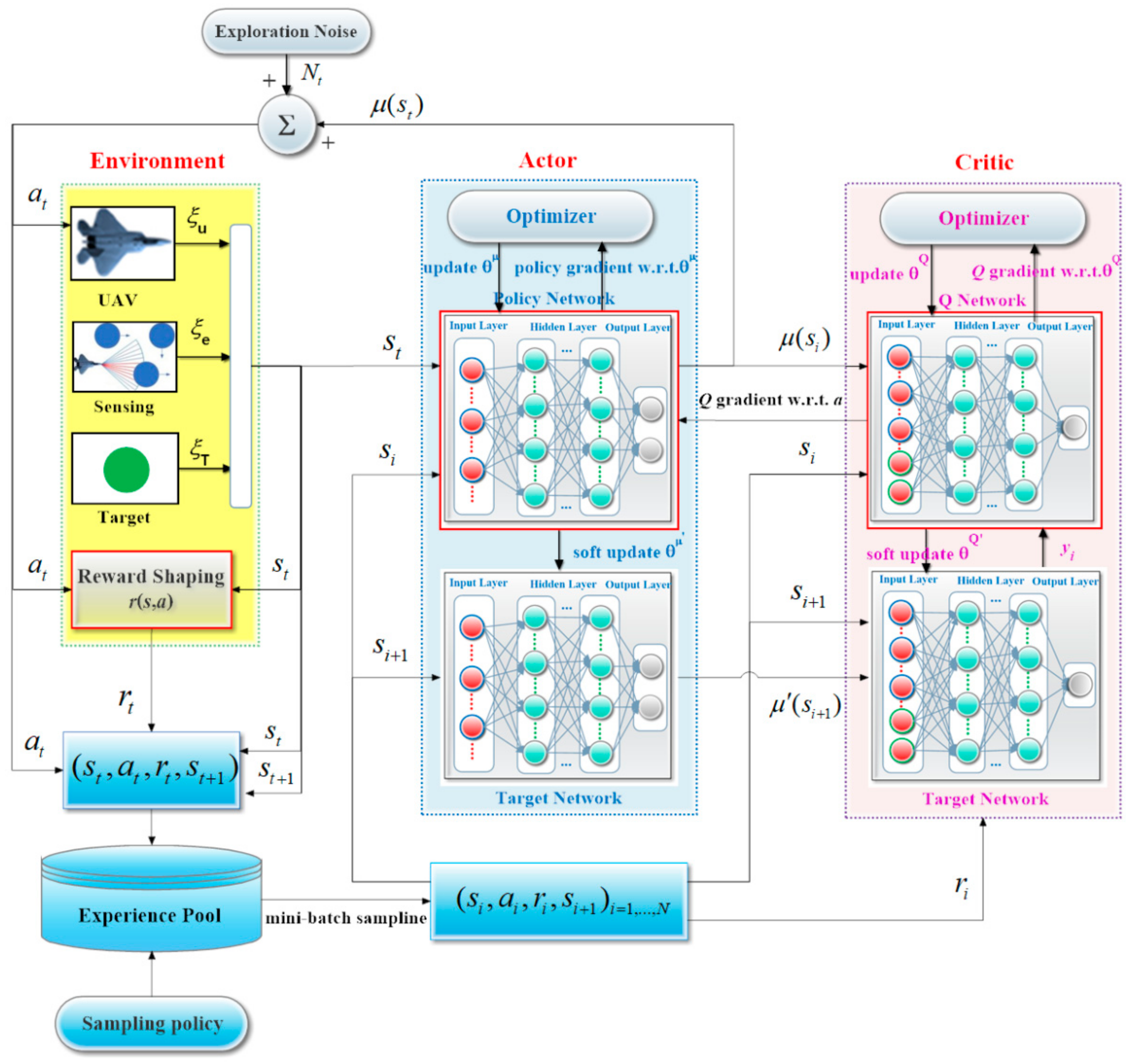
(1) We develop an actor-critic-based motion control framework, which can perform a dual-channel control of roll and speed, by predicting the desired steering angle and by reasoning the possible collision probability. The controller can provide safe flights for the UAV autonomously in dynamic uncertain environments.

(2) We propose an efficient policy-based DRL algorithm, Robust-DDPG, in which three critical tricks are introduced to provide a robust controller for the UAV. The first is a delayed-learning trick, in which the critic and actor networks are batch updated after each episode finishes, rather than being updated in each iteration. The second is an adversarial-attack trick, in which an adversarial scheme is introduced to sample noisy states and actions in the learning process. This trick will increase the robustness of the trained networks. The last is a mixed-exploration trick, in which rough sampling, based on $ϵ$-greedy and a fine sampling, based on Gaussian are performed in different periods of learning. By combining these three tricks, Robust-DDPG is able to overcome the shortcomings of DDPG and provide the UAV a controller with better adaptability to complicated, dynamic, and uncertain environments.

(3) We constructed a UAV mission platform to simulate dynamic stochastic environments for training and evaluating the effectiveness and robustness of our proposed methods. Through a series of experiments, we show that our trained UAV can adapt to various dynamic uncertain environments, with neither a map of the environment nor retraining or fine-tuning.

The remainder of this paper is organized as follows. Section 2 introduces the UAV motion control problem and formulates it as an MDP. Section 3 elaborates the core approach, Robust-DDPG, for problem solving, where three improved tricks, delayed learning, adversarial attack, and mixed exploration are integrated into an actor-critic framework. The performance, effectiveness, and adaptability of the proposed algorithm are demonstrated through a series of experiments in Section 4. Section 5 conducts a further discussion about the experimental results. Section 6 concludes this paper and envisages some future work.

2. Problem Formulation

2.1. UAV Motion Control

2.1.1. Kinematics of UAV

Six degrees of freedom (DoF) aircraft model is the most accurate in UAV’s flight control. However, it is taken that the UAV owns an onboard autopilot that will provide the low-level flight controls in a fast-inner loop and maintain roll, pitch, and yaw stability for the UAV, as well as velocity tracking and altitude holding functions [34,35]. For the sake of brevity and without loss of generality, we adopt the kinematics model with four DoF as a substitute for the six DoF one and apply it in the design of a high-level controller of the UAV. In our kinematics, we assume the UAV flies at a constant altitude and fly with inertial coordinated turns, in which the bank angle is set so that the centrifugal force acting on the aircraft is equal and opposite to the horizontal component of the lift acting in the radial direction [36]. These assumptions are reasonable in many realistic cases and can allow us to focus more on the motion control algorithms.

Let ${\mathit{p}}_u:=\left(x_u,y_u\right)$ and ${\dot{\mathit{p}}}_u:=\left({\dot{x}}_u,{\dot{y}}_u\right)$ denote the planar position and velocity in Cartesian inertial coordinates, respectively. By taking some additional disturbances into account, the continuous-time kinematics of our UAV reads [37],

$$\frac{d}{dt}\left(\begin{array}{c}{x}_u\\ y_u\\ {\psi }_u\\ {\varphi }_u\end{array}\right)=\left(\begin{array}{c}{v}_u\cos {\psi }_u+{\eta }_{\dot{x}}\\ v_u\sin {\psi }_u+{\eta }_{\dot{y}}\\ -\left(g/v_u\right)\tan {\varphi }_u+{\eta }_{\dot{\psi }}\\ f\left({\varphi }_u,a_{\varphi }\right)\end{array}\right)$$

(1)

where $g$ denotes the acceleration due to gravity. ${\psi }_u$, ${\varphi }_u$ denote the heading angle and roll angle, and $v_u$ denotes the linear velocity of the UAV. ${\eta }_{\dot{x}},{\eta }_{\dot{y}},{\eta }_{\dot{\psi }}$ are the disturbance terms due to velocity and heading rate, which is drawn from normal distributions $N\left(0,{\sigma }_{\dot{x}}^2\right)$, $N\left(0,{\sigma }_{\dot{y}}^2\right)$, and $N\left(0,{\sigma }_{\dot{\psi }}^2\right)$ respectively. By introducing these stochastic factors into the states of the model, we can partly make up for the loss of the un-modelled dynamics. The function $f\left({\varphi }_u,u_{\varphi }\right)$ defines the roll dynamics, which depends on a specific problem. The negative sign in the third row indicates the different definitions of the roll and heading direction, where the clockwise direction is defined as a positive roll, while the clockwise direction produces a negative roll.

2.1.2. Dual-Channel Control for UAV

Mobility control of a fixed-wing UAV in real environments could be complex, especially when the environment is unknown and changing rapidly. In our scenario, a fixed-wing UAV is supposed to have to fly across a dynamic unknown area until a specified target is finally reached. It is such an arduous circumstance for the UAV because of the ubiquitous mobile threats. Unlike most navigation researches that only considered a heading control [30,31] for the UAV, we utilize a dual-channel control to provide the UAV better flight robustness. As the increased speed control channel offers more avoiding options for the UAV when faced with dynamic environments.

Let ${\mathit{a}}_t={\left[a_{v,t},a_{\varphi ,t}\right]}^T$ be the control vector for the UAV at time $t$, in which $a_{v,t}$ and $a_{\varphi ,t}$ are the control commands due to the speed, and the roll, respectively. $a_{v,t}$ is represented as the probability of collision that can be used to modulate the forward speed of the UAV [1], while $a_{\varphi ,t}$ is the steering rate that can turn current roll to the desired one. Specifically, low-pass filters are used to provide soft updates of the speed and roll angle as,

$$\left\{\begin{array}{l}{v}_{u,t}=\left(1-{\lambda }_v\right)v_{u,t-1}+{\lambda }_v\left(1-a_{v,t}\right)v_{u,max}\\ {\varphi }_{u,t}=\left(1-{\lambda }_{\varphi }\right){\varphi }_{u,t-1}+{\lambda }_{\varphi }{a}_{\varphi ,t}{\varphi }_{u,max}\end{array}\right.$$

(2)

where ${\lambda }_v$ and ${\lambda }_{\varphi }$ are the tuning factors selected empirically for trading off smoothness and reactiveness of the flight. From the speed controller, we conclude that the UAV will gradually accelerate to maximal speed $v_{u,max}$ if the collision probability $a_{v,t}$ is 0, and will slow down to 0 when $a_{v,t}$ closes to 1. Similarly, the roll controller can map the predicted steering rate $a_{\varphi ,t}$ into a desired roll angle ${\varphi }_{u,t}$. Once the speed and roll are updated, the UAV moves to a new position by integrating Equation (1).

2.2. UAV Motion Control as an MDP

To provide the UAV with a robust controller to adapt to dynamic uncertain environments, we focus on the reinforcement learning technique. RL uses a Markov decision process (MDP) [31,38] to model the controller, in which the problem is abstracted into an Agent and an Environment. The agent can learn optimal sequential control policies from the historical trajectories accumulated by trial-and-error interactions with the environment. At each time step, the agent perceives the current system state $\mathit{s}\in \mathit{S}$ and selects a favorable action $\mathit{a}\in \mathit{A}$ depending on $\mathit{s}$ and its knowledge about past experiences. After applying this action $\mathit{a}$ to the UAV, a new system state ${\mathit{s}}^{\prime }\in \mathit{S}$ and a reward signal $\mathit{r}$ will arrive to the agent, and then the cycle repeats. Figure 1 illustrates the RL-based motion control structure of the UAV. The state $\mathit{s}$, action $\mathit{a}$ and reward $\mathit{r}$ constitute the core elements of the controller.

2.2.1. State and Action Specification

The state represents a collection of all the information that UAV can obtain. In this paper, onboard GPS and gyroscope devices can provide the agent its state ${\mathit{\xi }}_{\mathit{u}}={\left[x_u,y_u,{\dot{x}}_u,{\dot{y}}_u,{\psi }_u,{\varphi }_u\right]}^T$ in real-time, where $\left(x_u,y_u\right)$ is the planar position, $\left({\dot{x}}_u,{\dot{y}}_u\right)$ is the planar speed, ${\psi }_u$ is the heading, and ${\varphi }_u$ is the roll angle of the UAV. A LiDAR [39] with ${\mathrm{N}}_{\mathrm{r}}$ rays is equipped on the UAV to keep sensing the changing of the surroundings. At each sampling moment, the agent will receive a feedback of the environment state ${\mathit{\xi }}_{\mathit{e}}={\left[d_1,d_2,\dots ,d_{N_r}\right]}^T$, where $d_i$ denotes the detected relative distance between the UAV and the threats by the $i$-th ray (depicted in Figure 2). Besides, the target state ${\mathit{\xi }}_{\mathit{T}}={\left[x_T,y_T\right]}^T$ is supposed to be transmitted to the agent by an indicator-like device periodically, where $\left(x_T,y_T\right)$ represents the position of the target. Then, we get the system state $\mathit{s}$ by combining ${\mathit{\xi }}_{\mathit{u}}$, ${\mathit{\xi }}_{\mathit{e}}$ and ${\mathit{\xi }}_{\mathit{T}}$, i.e.,

$$\mathit{s}={\left[x_u,y_u,{\dot{x}}_u,{\dot{y}}_u,{\psi }_u,{\varphi }_u,d_1,d_2,\dots ,d_{N_r},x_T,y_T\right]}^T$$

(3)

The fixed-wing UAV maneuvers by selecting its appropriate speed and roll control commands, and holding them for one second or until the next commands are selected. In our scenario, the two control commands are represented by action $\mathit{a}={\left[a_v,a_{\varphi }\right]}^T$, where $a_v\in \left[0,1\right]$ denotes the probability of collision that can be estimated to control the forward speed of the UAV, while $a_{\varphi }\in \left[-1,1\right]$ is a steering signal that can be selected to turn the UAV to the desired roll angle.

2.2.2. Reward Shaping

Reward $r\left(\mathit{s},\mathit{a}\right)$ acts as a signal evaluating how good it is when taking an action $\mathit{a}$ at a state $\mathit{s}$ [31]. The rewards are the only feedback signals available for the agent’s learning. Accordingly, a well-shaped reward function should contain as many useful human experiences as possible. In this paper, we abandon the normally used sparse reward and shape a non-sparse reward scheme [40] that incorporates our domain knowledge about the motion control problem to precisely describe the tiny impart of selected policy. Four basic experiences are considered to construct the non-sparse reward: A) The UAV is urged to fly to the target; any action that brings the UAV close to the target should be rewarded and be punished if it is driven away from the target, and the faster the approaching or leaving, the greater the reward or penalty; B) the UAV is required to complete the mission as soon as possible, a greater approaching speed deserves a greater reward; C) the UAV should fly towards the target, any deviation from the target direction should be punished; D) the UAV should be proactive in avoiding collisions with the threats, if it is quickly approaching a threat, a great penalty should be assigned to remind the UAV to slow down or turn immediately. We have formulated these four experiences as follows,

$$r_A=D_{ut}^{pre}-D_{ut}^{cur}$$

(4)

$$r_B=\left(v_u/v_{u,max}\right)\times \cos \mathsf{\Delta }\psi$$

(5)

$$r_C=-\mathsf{\Delta }\psi /4$$

(6)

$$r_D=\left(v_u/v_{u,max}\right)\times \left(D_f/D_s-1\right)$$

(7)

where $D_{ut}^{pre},D_{ut}^{cur}$ denote the previous and current relative distances between UAV and the target; $\mathsf{\Delta }\psi$ denotes the angle of the UAV flight direction deviating from the target; $v_u$ are the current speeds of the UAV; $D_s$ is the detection distance of the sensor; $D_f$ is the distance of the detected threat in front of the UAV and if there is no threat ahead of it, $D_f$ will be set to $D_s$. All the variables can be found in Figure 3. From the above four equations, we can see that $r_A$ is a reward item when $D_{ut}^{pre}>D_{ut}^{cur}$, otherwise, it is a penalty, and $r_B$ is always a reward while $r_C$ and $r_D$ are penalties. To summarize, the reward function can be finally formulated as,

$$r\left(\mathit{s},\mathit{a}\right)={\mu }_1{r}_A+{\mu }_2{r}_B+{\mu }_3{r}_C+{\mu }_4{r}_D$$

(8)

where ${\mu }_1,{\mu }_2,{\mu }_3,{\mu }_3$ are used to indicate the contribution rates of the four items, ${{\displaystyle \sum }}_{i=1}^4{\mu }_i=1$.

2.2.3. Non-Myopic Objective

As for a reinforcement learning setup, state space $\mathit{S}$, action space $\mathit{A}$, reward function $r\left(\mathit{s},\mathit{a}\right)$ and transition dynamics $\mathit{p}\left({\mathit{s}}^{\prime }|\mathit{s},\mathit{a}\right)$ consist as a standard MDP. Unlike traditional myopic methods that make decisions rely only on the immediate reward $r$, RL learns an optimal control policy $\pi$ by maximizing a non-myopic objective,

$$J_{\pi }={\mathbb{E}}_{{\mathit{s}}_i~\mathit{p},{\mathit{a}}_i~\pi }\left[{\displaystyle \sum }_{i=0}^H{\gamma }^{i}r\left({\mathit{s}}_i,{\mathit{a}}_i\right)\right]$$

(9)

where ${\displaystyle \sum }_{i=0}^H{\gamma }^{i}r\left({\mathit{s}}_i,{\mathit{a}}_i\right)$ is a discounted future reward with a discounting factor $\gamma \in \left[0,1\right]$. $H$ is the horizon of the prediction. The policy $\pi$ is defined to map system states to a probability distribution over the actions $\pi :\mathit{S}\to \mathit{P}\left(\mathit{A}\right)$. For an arbitrary pair (${\mathit{s}}_t,{\mathit{a}}_t$), $Q$-function is defined to describe the expected long-term cumulative return when performing an action ${\mathit{a}}_t$ in state ${\mathit{s}}_t$ and following $\pi$:

$$\begin{array}{cc}\hfill Q_{\pi }\left({\mathit{s}}_t,{\mathit{a}}_t\right)& ={\mathbb{E}}_{{\mathit{s}}_i~\mathit{p},{\mathit{a}}_i~\pi }\left[{\displaystyle \sum }_{i=t}^H{\gamma }^{i-t}r\left({\mathit{s}}_i,{\mathit{a}}_i\right)|{\mathit{s}}_t,{\mathit{a}}_t\right]\hfill \\ & ={\mathbb{E}}_{{\mathit{s}}_{t+1}~\mathit{p}}\left[r\left({\mathit{s}}_t,{\mathit{a}}_t\right)+\gamma {\mathbb{E}}_{{\mathit{a}}_{t+1}~\pi }\left[Q_{\pi }\left({\mathit{s}}_{t+1},{\mathit{a}}_{t+1}\right)\right]\right]\hfill \end{array}$$

(10)

Subsequently, the optimal action can be determined by:

$${\mathit{a}}_{\mathit{t}}^{*}= \arg \underset{\mathit{a}}{\max }{Q}_{\pi }\left({\mathit{s}}_t,{\mathit{a}}_t\right).$$

(11)

Despite the non-myopic scheme described above can provide a robust control policy by fully considering its impact on the future, it is troubled by the curse of dimensionality while trying to calculate the Q-value. As the agent is facing continuous state space and continuous action space in our scenario, and more seriously, the transition dynamics $\mathit{p}\left({\mathit{s}}^{\prime }|\mathit{s},\mathit{a}\right)$ is unknown to the agent. Any heuristic or evolutionary algorithms become intractable for solving the Equation (11). To address it, we design a deep neural network, $\mu (\mathit{s}|{\mathit{\theta }}^{\mu })$, to approximate the function of $\arg \underset{\mathit{a}}{\max }{Q}_{\pi }\left({\mathit{s}}_t,{\mathit{a}}_t\right)$, where the deep neural network could directly map high-dimensional continuous state ${\mathit{s}}_t$ into optimal action ${\mathit{a}}_t$. (As illustrated in Figure 4)

$${\mathit{a}}_{\mathit{t}}^{*}\leftarrow \mu ({\mathit{s}}_t|{\mathit{\theta }}^{\mu })$$

(12)

As we can see in Figure 4, by approximating, the intractable planning problem (Equation (11)) is simplified into a deep neural network training problem, i.e., to figure out optimal parameters ${\mathit{\theta }}^{\mu }$ of $\mu (\mathit{s}|{\mathit{\theta }}^{\mu })$. In Section 3, we spend the whole section to describe the specific learning framework and learning techniques.

3. Robust-DDPG for UAV Motion Control

This section introduces an actor-critic framework to training the agent described in Section 2, and a novel DRL algorithm is proposed to address challenges belongs to traditional DDPG and used to provide the UAV robust end-to-end motion control strategies.

3.1. Actor-Critic Framework

As shown in Section 2, the UAV motion control problem is modeled with a continuous state space and a continuous action space, which turns Q-learning [15] and Deep Q-learning (DQN) [19] unavailable because of their poor efficiencies in representing a continuous policy. Instead, an actor-critic approach is considered in this research. As depicted in Figure 5, the actor-critic approach expands DQN with a deterministic parameterized actor function $\mu (\mathit{s}|{\mathit{\theta }}^{\mu })$, which defines the policy by deterministically mapping a state to a specific action, i.e., $\mathit{a}=\mu (\mathit{s}|{\mathit{\theta }}^{\mu })$. By replacing policy gradient (PD) [15] $\mathit{a}~\pi (\mathit{s}|{\mathit{\theta }}^{\pi })$ with deterministic policy gradient (DPG) [28] $\mathit{a}=\mu (\mathit{s}|{\mathit{\theta }}^{\mu })$, the agent will learn an optimal policy without any action sampling and action integrating in each iteration. It is a practical technique to handle problems with continuous high-dimensional action spaces. Specifically, a deep neural network with parameter ${\mathit{\theta }}^{\mu }$ is used as an approximator (red box in actor module in Figure 5) for the actor, inspired by DQN that exploits a parameterized deep neural network $Q(\mathit{s},\mathit{a}|{\mathit{\theta }}^Q)$ (red box in critic module in Figure 5) to approximate Q-function in Equation (10). To disrupt the correlation between samples and maintain stable learning, experience replay strategy (blue modules in Figure 5) and two fixed target networks, ${\mu }^{\prime }(\mathit{s}|{\mathit{\theta }}^{{\mu }^{\prime }})$ and $Q^{\prime }(\mathit{s},\mathit{a}|{\mathit{\theta }}^{Q^{\prime }})$ (white boxes in actor and critic modules in Figure 5) are created to provide target signals for critic updating.

The representative algorithm with this actor-critic framework is deep deterministic policy gradient (DDPG) [29]. With this framework, the agent can learn by interacting with the environment repeatedly until a robust policy network $\mu (\mathit{s}|{\mathit{\theta }}^{\mu })$ is obtained. At each time step $t$, the agent receives observation ${\mathit{s}}_t$ and selects an action by ${\mathit{a}}_t=\mu \left({\mathit{s}}_t|{\mathit{\theta }}^{\mu }\right)+N_t$, where $N_t$ is the exploration noise. Then, the action ${\mathit{a}}_t$ is applied to control the UAV to fly and a reward $r_t$ returns and a new state ${\mathit{s}}_{t+1}$ is observed. The transition $({\mathit{s}}_t,{\mathit{a}}_t,r_t,{\mathit{s}}_{t+1}$) is then stored in experience pool. Afterwards, a mini-batch of N transitions ${\left({\mathit{s}}_i,{\mathit{a}}_i,r_i,{\mathit{s}}_{i+1}\right)}_N$ is sampled from the pool to calculate two gradients:

$${\nabla }_{{\mathit{\theta }}^Q}L=-\frac{1}{N}{{\displaystyle \sum }}_{i=1}^N\left(y_i-Q\left({\mathit{s}}_i,{\mathit{a}}_i|{\mathit{\theta }}^Q\right)\right){\nabla }_{{\mathit{\theta }}^Q}Q\left(\mathit{s},\mathit{a}|{\mathit{\theta }}^Q\right){|}_{\mathit{s}={\mathit{s}}_i,\mathit{a}={\mathit{a}}_i}$$

(13)

$${\nabla }_{{\mathit{\theta }}^{\mu }}J\approx \frac{1}{N}{{\displaystyle \sum }}_{i=1}^N{\nabla }_{\mathit{a}}Q\left(\mathit{s},\mathit{a}|{\mathit{\theta }}^Q\right){|}_{\mathit{s}={\mathit{s}}_i,\mathit{a}=\mu \left({\mathit{s}}_i\right)}{\nabla }_{{\mathit{\theta }}^{\mu }}\mu \left(\mathit{s}|{\mathit{\theta }}^{\mu }\right){|}_{\mathit{s}={\mathit{s}}_i}$$

(14)

where $y_i=r_i+\gamma Q^{\prime }\left({\mathit{s}}_{i+1},{\mu }^{\prime }\left({\mathit{s}}_{i+1}|{\mathit{\theta }}^{{\mu }^{\prime }}\right)|{\mathit{\theta }}^{Q^{\prime }}\right)$ is the target signal of the critic. The two gradients are then used to update Q network parameter ${\mathit{\theta }}^Q$ and policy network parameter ${\mathit{\theta }}^{\mu }$, respectively. At last, the two target network parameters ${\mathit{\theta }}^{Q^{\prime }}$ and ${\mathit{\theta }}^{{\mu }^{\prime }}$ are updated by soft or hard update strategies.

3.2. Robust Learning Techniques

Within the actor-critic framework, DDPG could handle problems with both high-dimensional continuous state space and high-dimensional continuous action space. However, DDPG often acts precariously since it is brittle with respect to hyper-parameters and environments, and any small perturbation may make it breaking. It is risky to directly apply such an unstable model as the motion controller of the UAV. In this work, we propose an improved approach, Robust-DDPG, to address issues of DDPG by introducing a delayed-learning trick, an adversarial-attack trick, and a combined-exploration trick.

3.2.1. Delayed Learning Trick

As we are aware, the original DDPG adopts a direct updating scheme in the learning process, in which both the critic and actor parameters are updated at each time step. Theoretically, direct update produces more training steps and could accelerate the convergence, but it often leads to unstable agents and policy jittering occurs occasionally, while exploiting it in practical applications. Scott et al. [41] have blamed the failures on accumulating errors of the estimated Q-function and proposed a Twin Delayed DDPG (TD3) approach to address it. To the best of our knowledge, the underlying reason is that the traditional training method of DDPG changes the strategic direction of the policy too frequently, which in return confuses the agent in policy learning. Here, let’s take the UAV motion control as an example to illustrate this intuition. For a given state, there lie two policies for UAV to choose: A sound policy with low speed and small turn that maintain the UAV get as few collision penalties as possible and a radical policy with high speed and big turn that let the UAV finish the task as soon as possible. Both policies may benefit the UAV with high rewards. In other words, with a changed strategic direction, the learned critic may provide similar evaluations for two completely different policies, and if the changing happens frequently, the actor will get lost in the learning.

To address this drawback, a delayed learning trick is designed here. Differ from the policy delay in TD3, our trick delays the actor and critic network learning operations to the end of each episode. This way ensures the actor and the critic to obey the same principle in an ongoing episode and after each episode finishes, intensive learning begins. Since it avoids the repeatedly changing of strategic direction, this trick could stabilize the training to a certain extent. In addition, a fixed interval is set for the soft updates of the target networks. A quick procedure of delayed leaning trick for DDPG is depicted in Algorithm 1.

Algorithm 1: Delayed learning trick (with DDPG)

1: for episode = 1, M do

2: reset environment and receive initial observation state ${\mathit{s}}_1$

3: while not collide and not target and $t<T$ do

4:  select action $a_t$ according to policy and exploration

5:  execute action $a_t$ and observe new state ${\mathit{s}}_{t+1}$ and reward $r_t$

6:  store transition (${\mathit{s}}_t,a_t,r_t,{\mathit{s}}_{t+1}$) in experience pool

7: end while

8: for $l=1,t$ do //Delayed Learning

9:  sample a random mini-batch of N transitions ${\left({\mathit{s}}_i,a_i,r_i,{\mathit{s}}_{i+1}\right)}_{i=1,N}$

10:  update critic network weights using gradient in Equation (12)

11:  update actor network weights using gradient in Equation (13)

12:  if target update interval reaches do

13:   soft update target network weights of critic and actor

14:  end if

15: end for

16: end for

3.2.2. Adversarial Attack Trick

Most DRL algorithms are trained with ideal virtual environments, but there are ubiquitous noises in realistic applications. It has been shown that the ideally trained agent can be easily fooled into wrong policies by perturbing the input with adversarial noises [42]. For some safety critical domains, i.e., UAVs and robotics, robustness assumes much greater importance that a tiny adversarial noise may lead to undesirable and hazardous results.

To train a robust agent that enables successful adaptions of the real-world variations, an adversarial attack trick is introduced into the learning process of the DDPG. An adversarial attack is defined as any possible perturbation that could cause a trained agent to fail [43]. More specifically, an attack mechanism is designed to generate random noise and add it to current observations of the state with the hope that these noise samples will fool the agent to take bad actions. Algorithm 2 outlines the adversarial attack trick for DDPG, where the current state $\mathit{s}$, the trained critic target $Q^{\prime }\left(\mathit{s},\mathit{a}|{\mathit{\theta }}^{Q^{\prime }}\right)$, the trained actor $\mu \left(\mathit{s}|{\mathit{\theta }}^{\mu }\right)$ constitute the inputs and the corrupted state ${\mathit{s}}_{noi\mathit{s}e}$ forms the output. The main idea behind the attack is to search repeatedly nearby the current state $\mathit{s}$ until the state that makes the agent select the worst action ${\mathit{s}}_{noi\mathit{s}e}$ is finally found. An adversarial deep $N_{\mathit{a}}$ can be assigned. All the noises are sampled from a Gaussian distribution with a standard deviation ${\sigma }_{\mathit{s}}$ in the attack. Algorithm 2 outlines the specific procedure of adversarial attack trick.

Algorithm 2: Adversarial attack trick (with DDPG)

1: $St\mathit{a}teAtt\mathit{a}ck\left(Q^{\prime }\left(\mathit{s},\mathit{a}|{\mathit{\theta }}^{Q^{\prime }}\right),\mu \left(\mathit{s}|{\mathit{\theta }}^{\mu }\right),\mathit{s}\right)$

2: ${\mathit{a}}^{*}=\mu \left(\mathit{s}|{\mathit{\theta }}^{\mu }\right)$, $Q^{*}=Q^{\prime }\left(\mathit{s},{\mathit{a}}^{*}|{\mathit{\theta }}^{Q^{\prime }}\right)$

3: for $i=1,N_{\mathit{a}}$ do

4:  ${\mathit{s}}_{noi\mathit{s}e}=\mathit{s}+G\mathit{a}u\mathit{s}\mathit{s}i\mathit{a}n\left(0,{\sigma }_{\mathit{s}}^2\right)$

5:  ${\mathit{a}}_{noi\mathit{s}e}=\mu \left({\mathit{s}}_{noi\mathit{s}e}|{\mathit{\theta }}^{\mu }\right)$, $Q_{noi\mathit{s}e}=Q^{\prime }\left(\mathit{s},{\mathit{a}}_{noi\mathit{s}e}|{\mathit{\theta }}^{Q^{\prime }}\right)$

6:  if $Q_{noi\mathit{s}e}<Q^{*}$ then

7:   $Q^{*}=Q_{noi\mathit{s}e}$, $\mathit{s}={\mathit{s}}_{noi\mathit{s}e}$

8:  end if

9: end for

10: return ${\mathit{s}}_{noi\mathit{s}e}$

By modeling the uncertainties of the real world, an adversarial attack could improve the robustness of DDPG when it is utilized to construct the motion controller of the UAV.

3.2.3. Mixed Exploration Trick

A major challenge of learning in continuous action spaces is exploration. DDPG constructs an exploration action ${\mathit{a}}_t$ by adding noise $N_t$ sampled from an Ornstein-Uhlenbeck (OU) process to online policy $\mu \left({\mathit{s}}_t|{\mathit{\theta }}^{\mu }\right)$. That is:

$${\mathit{a}}_t=\mathrm{clip}\left(\mu \left({\mathit{s}}_t|{\mathit{\theta }}^{\mu }\right)+N_t,{\mathit{a}}_{low},{\mathit{a}}_{high}\right), N_t\sim OU\left(u,\vartheta ,\sigma \right)$$

(15)

where $\mathrm{clip}\left(·\right)$ is a clipping function that limits ${\mathit{a}}_t$ in $\left[{\mathit{a}}_{low},{\mathit{a}}_{high}\right]$. This scheme can produce temporally correlated exploration and is efficient for continuous physical control problems theoretically [29]. However, the actual effect varies depending on the selected parameters $\left(u,\vartheta ,\sigma \right)$ in practical applications. For example, at the start of training, we usually need differentiated action samples to ensure efficient learning, which means a bigger $\sigma$ is required so that noises with enough deviations can be yielded. But the reality is, a bigger $\sigma$ produces a large proportion of actions stay at the margin of ${\mathit{a}}_{low}$ or ${\mathit{a}}_{high}$ by clipping. It is these bad samples that have drag the DDPG down in the learning efficiency and exploiting stability. To cope with this drawback, we adopt a mixed exploration strategy in this paper. Specifically, a dynamic $ϵ$-greedy is used to provide a rough exploration at the start of training and an OU is adopted to conduct a fine exploration in the following training stages. $ϵ$-greedy’s direct sampling from a Uniform distribution maintains sufficient sample diversity and facilitates a fast convergence. The main idea of the mixed exploration trick is described in Algorithm 3.

Algorithm 3: Mixed exploration trick (with DDPG)

1: $ActionExplore\left(\mu \left(\mathit{s}|{\mathit{\theta }}^{\mu }\right),{\mathit{s}}_t,{ϵ}_t\right)$

2: if rand < ${ϵ}_t$ do

3:  ${\mathit{a}}_t=Uniform\left({\mathit{a}}_{low},{\mathit{a}}_{high}\right)$

4: else do

5:  ${\mathit{a}}_t=\mu \left({\mathit{s}}_t|{\mathit{\theta }}^{\mu }\right)+OU\left(u,\vartheta ,\sigma \right)$

6:  ${\mathit{a}}_t=clip\left({\mathit{a}}_t,{\mathit{a}}_{low},{\mathit{a}}_{high}\right)$

7: end if

8: return ${\mathit{a}}_t$

3.2.4. Overall Robust-DDPG Algorithm

Ultimately, we present the robust deep deterministic policy gradient algorithm (Robust-DDPG) by introducing the delayed learning trick, the adversarial attack trick and the mixed exploration trick described in Section 3.2.1, Section 3.2.2 and Section 3.2.3 into DDPG. Robust-DDPG is summarized in Algorithm 4.

Algorithm 4: Robust-DDPG

1: randomly initialize critic network $Q\left(\mathit{s},\mathit{a}|{\mathit{\theta }}^Q\right)$ and actor $\mu \left(\mathit{s}|{\mathit{\theta }}^{\mu }\right)$ with weights ${\mathit{\theta }}^Q$ and ${\mathit{\theta }}^{\mu }$

2: initialize target network $Q^{\prime }\left(\mathit{s},\mathit{a}|{\mathit{\theta }}^{Q^{\prime }}\right)$ and ${\mu }^{\prime }\left(\mathit{s}|{\mathit{\theta }}^{{\mu }^{\prime }}\right)$ with weights ${\mathit{\theta }}^{Q^{\prime }}\leftarrow {\mathit{\theta }}^Q, {\mathit{\theta }}^{{\mu }^{\prime }}\leftarrow {\mathit{\theta }}^{\mu }$

3: initialize hyper-parameters: attack point A, experience pool D, batch size N, target update interval K

4: for $e=1,E$ do

5: reset environment and receive initial observation state ${\mathit{s}}_1$

6: while not collide and not target and $t<T$ do

7:  if $e\ge A$ do

8:   start an adversarial attack by ${\mathit{s}}_t^{\prime }\leftarrow St\mathit{a}teAtt\mathit{a}ck\left(Q^{\prime }\left(\mathit{s},\mathit{a}|{\mathit{\theta }}^{Q^{\prime }}\right),\mu \left(\mathit{s}|{\mathit{\theta }}^{\mu }\right),{\mathit{s}}_t\right)$

9:   select action through mixed exploration ${\mathit{a}}_t\leftarrow ActionExplore\left(\mu \left(\mathit{s}|{\mathit{\theta }}^{\mu }\right),{\mathit{s}}_t^{\prime },{ϵ}_t\right)$

10:  else do

11:   select action through mixed exploration ${\mathit{a}}_t\leftarrow ActionExplore\left(\mu \left(\mathit{s}|{\mathit{\theta }}^{\mu }\right),{\mathit{s}}_t,{ϵ}_t\right)$

12:  end if

13:  execute action ${\mathit{a}}_t$ and observe new state ${\mathit{s}}_{t+1}$ and reward $r_t$

14:  store transition (${\mathit{s}}_t,{\mathit{a}}_t,r_t,{\mathit{s}}_{t+1}$) in D

15:  ${ϵ}_t\leftarrow \max \left({ϵ}_t-{\mathsf{\alpha }}_{\epsilon }\nabla \epsilon , {ϵ}_{min}\right)$, $t\leftarrow t+1$,

16: end while

17: for $l=1,t$ do //$Del\mathit{a}yed Le\mathit{a}rning$

18:  sample a random N transitions ${\left({\mathit{s}}_i,{\mathit{a}}_i,r_i,{\mathit{s}}_{i+1}\right)}_{i=1,N}$

19:  calculate gradient by ${\nabla }_{{\mathit{\theta }}^Q}L\leftarrow -N^{-1}{{\displaystyle \sum }}_i\left(y_i-Q\left({\mathit{s}}_i,{\mathit{a}}_i|{\mathit{\theta }}^Q\right)\right){\nabla }_{{\mathit{\theta }}^Q}Q\left(\mathit{s},\mathit{a}|{\mathit{\theta }}^Q\right){|}_{\mathit{s}={\mathit{s}}_i,\mathit{a}={\mathit{a}}_i}$

20:  calculate gradient by ${\nabla }_{{\mathit{\theta }}^{\mu }}J\leftarrow N^{-1}{{\displaystyle \sum }}_i{\nabla }_{\mathit{a}}Q\left(\mathit{s},\mathit{a}|{\mathit{\theta }}^Q\right){|}_{\mathit{s}={\mathit{s}}_i,\mathit{a}=\mu \left({\mathit{s}}_i\right)}{\nabla }_{{\mathit{\theta }}^{\mu }}\mu \left(\mathit{s}|{\mathit{\theta }}^{\mu }\right){|}_{\mathit{s}={\mathit{s}}_i}$

21:  update critic and actor weights by ${\mathit{\theta }}^Q\leftarrow {\mathit{\theta }}^Q-{\alpha }^Q{\nabla }_{{\mathit{\theta }}^Q}L$, ${\mathit{\theta }}^{\mu }\leftarrow {\mathit{\theta }}^{\mu }-{\alpha }^{\mu }{\nabla }_{{\mathit{\theta }}^{\mu }}J$

22:  if $l \% K=0$ do

23:   update target weights by ${\mathit{\theta }}^{Q^{\prime }}\leftarrow \tau {\mathit{\theta }}^Q+\left(1-\tau \right){\mathit{\theta }}^{Q^{\prime }}$, ${\mathit{\theta }}^{{\mu }^{\prime }}\leftarrow \tau {\mathit{\theta }}^{\mu }+\left(1-\tau \right){\mathit{\theta }}^{{\mu }^{\prime }}$

24:  end if

25: end for

26: end for

After thousands of training steps with Algorithm 4, the final policy network $\mu (\mathit{s}|{\mathit{\theta }}^{\mu })$ will be obtained and then it can continuously be utilized for autonomous motion control of UAV by ${\mathit{a}}_t=\mu ({\mathit{s}}_t|{\mathit{\theta }}^{\mu })$. Due to the three newly introduced tricks, the Robust-DDPG-based controller will theoretically provide better adaptabilities to complicated, dynamic, and uncertain environments, compared with the original DDPG algorithm.

4. Results

This section presents experiments for evaluating the performance, the effectiveness and the adaptability of the proposed robust motion controller of the UAV through training experiments, exploiting experiments, and generalization experiments.

4.1. Experimental Platform and Settings

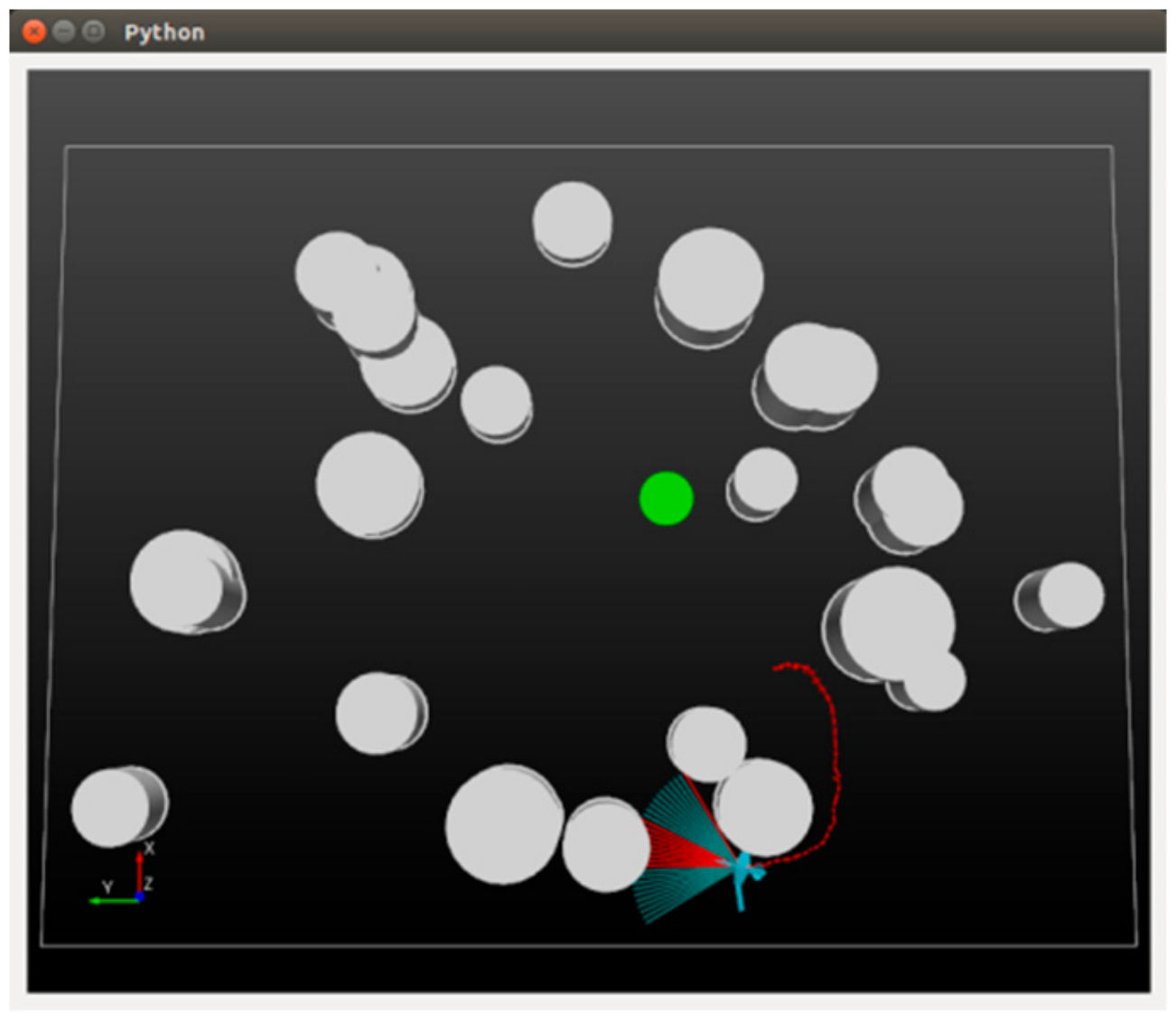
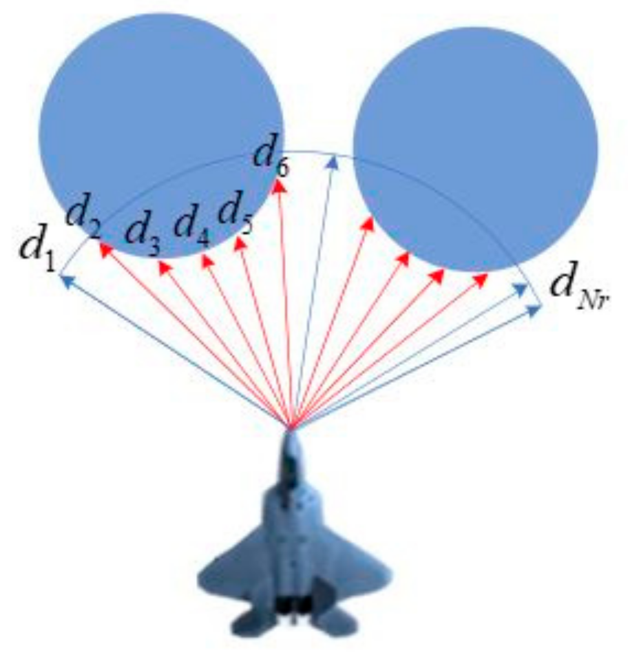
For the training and testing of the DRL-based motion controller, we construct a general simulation platform, depicted in Figure 6. The platform simulates a world with a total size of 400 $\times$ 300 m² (the rectangular area) and a series of threats (the 24 white cylinders with different heights and sizes) are randomly scattered in the world. A certain proportion of the threats are set to move with stochastic velocities obey a uniform distribution U(1,6). A fixed-wing UAV (the blue entity) is required to fly across the unknown world until a specified target (the green circle) is finally reached. The UAV is supposed to fly at an altitude of 100 m and be equipped with a sensor that is capable of detecting an area of 40 m ahead ($D_s=40$) and $\pm$45 degrees from left to right (the blue sector in front of the UAV). Whenever an object is detected, the corresponding blue beams will be set to red so that the user can intuitively see the interaction between the UAV and the environment. The mobility of the UAV is limited by a maximum velocity $v_{u,max}$ = 45 m/s and a maximum roll ${\varphi }_{u,max}=\pi /2$. The motion uncertainty of the UAV is considered by defining disturbances ${\sigma }_{\dot{x}}={\sigma }_{\dot{y}}=10$ and ${\sigma }_{\dot{\psi }}=5^{°}$. The reward contribution rates are instantiated as ${\mu }_1=0.3,{\mu }_2=0.4$ and ${\mu }_3={\mu }_4=0.15$.

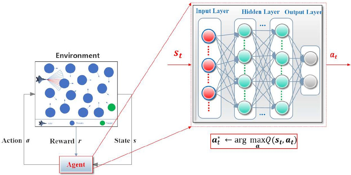
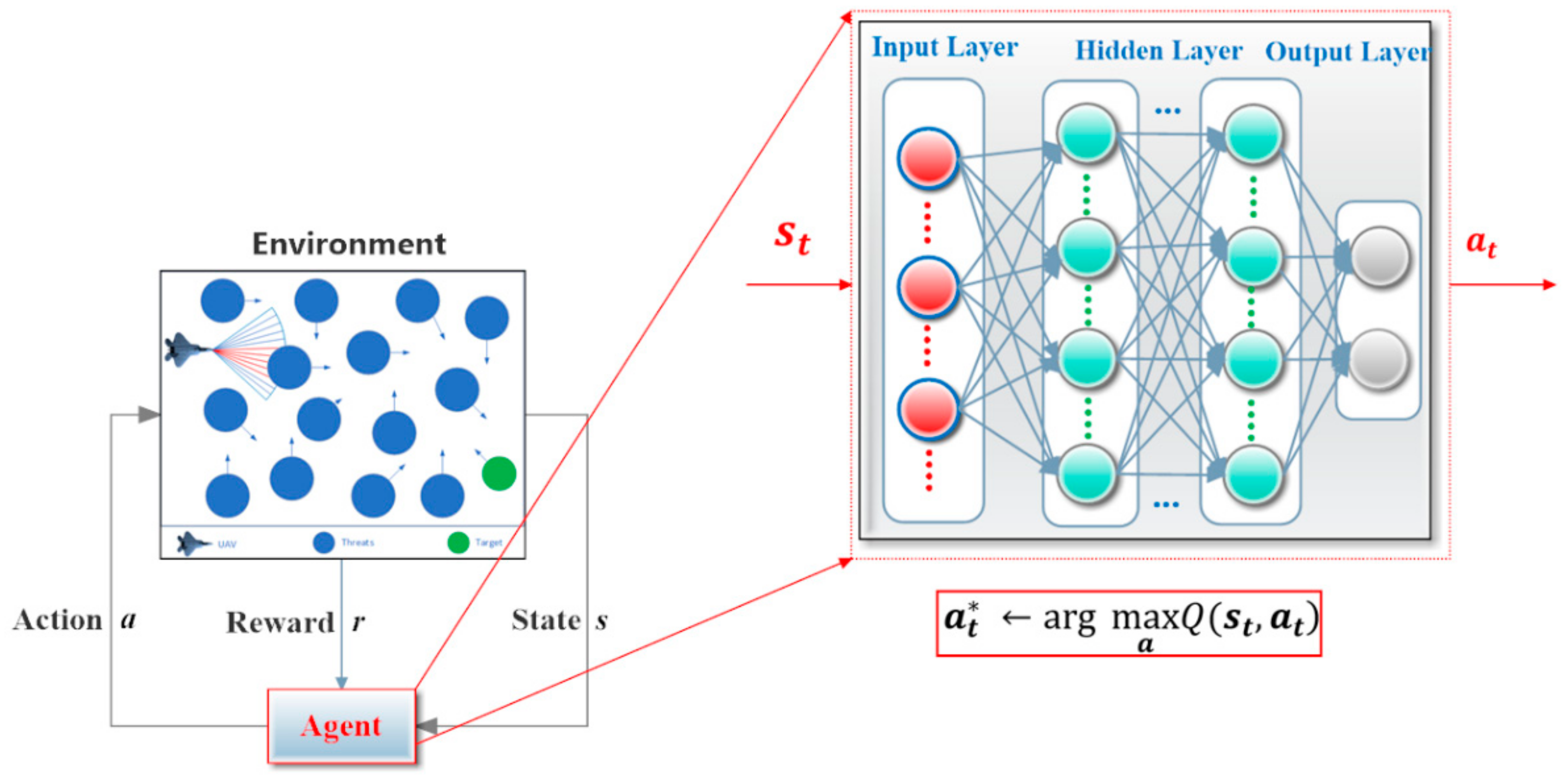
As described in Section 3.1, two neural networks constitute the core of the controller, in which the critic is constructed by a 40 $\times$ 100 $\times$ 100 $\times$ 1 fully connected neural network and the actor owns a structure of 38 $\times$ 100 $\times$ 100 $\times$ 2. The observed states are normalized as a 38-dimensional input to the actor and the two-dimensional output actions are used to control the UAV’s motion. Adam optimizer is employed to learn network parameters with the same learning rate of ${\alpha }^Q={\alpha }^{\mu }={10}^{-4}$ for the actor and critic. Other hyper-parameters are set with discount factor $\gamma =0.9$, batch size $N=256$, experience pool $D=10,000$, target update interval $K=200$, and attack point $A=4000$. In addition, the soft update tuning factor is $\tau =0.01$, the adversarial deep is $N_a=5$ and the standard deviation is ${\sigma }_s=0.5$. A descending $ϵ$-greedy of ${ϵ}_t=max\left({ϵ}_t-{\alpha }_{\epsilon }\nabla \epsilon , {ϵ}_{min}\right)$ mixed with an $\mathrm{OU}\left(u,\vartheta ,\sigma \right)$ distribution is used to explore the action spaces, where ${ϵ}_0=0.5, {\alpha }_{\epsilon }=0.0001$ and $\nabla \epsilon =0.4$ are set to provide a proper descending of $ϵ$ and ${ϵ}_{min}=0.0001$ sets the lower bound of $ϵ$. $u=0,\vartheta =0.15,$ and $\sigma =0.4$ are selected to generate temporally correlated explorations. Besides, the maximum episode length $T$ is set to 1000.

4.2. Experiment I: Performance of Robust-DDPG

Before its exploitation, the DRL-based controller has to be trained first. To demonstrate the performance of the proposed Robust-DDPG, reasonable comparative experiments are necessary. To be specific, we resort to another two state-of-the-art DRLs, DQN, and DDPG, as baselines and re-implement them with almost the same hyper-parameter settings to Robust-DDPG. In DQN, we assume the UAV flies at a constant velocity of 20 m/s and simplify the control commands to $a_{\varphi ,t}\in \left\{-1,0,1\right\}$ only. All three agents are trained with the same dynamic uncertain environment, depicted in Figure 5. The experiments repeat 7000 episodes with 5000 episodes for learning and 2000 episodes for exploiting. In each episode, the UAV, target, and threats are randomly re-deployed throughout the world.

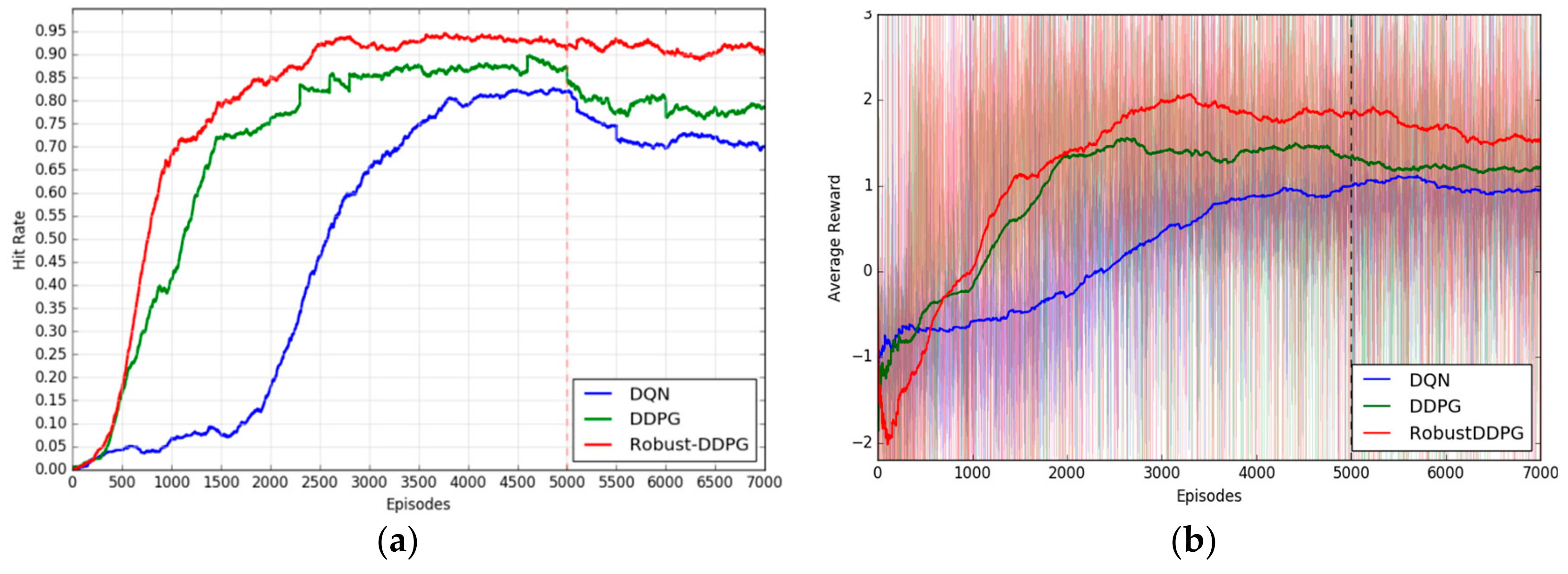
To measure the performance, we define some quantitative evaluation indicators: Hit rate, crash rate, lost rate, and average reward. For each agent, the hit rate, crash rate, and lost rate can be obtained by counting the percentage of successfully hitting the target over the latest 500 episodes, the percentage of crashing with threats over the last 500 episodes, and the percentage of trapped until that episode ends over the last 500 episodes, respectively. Average reward is defined as the mean value of the rewards per episode. Due to the severe fluctuation of average reward, we further average it every 500 episodes. The final learning results are illustrated in Figure 7, including convergence curves of the hit rate (Figure 7a) and the convergence curves of the average reward (Figure 7b).

From Figure 7, we can see: (1) Robust-DDPG uses about 2500 episodes to converge to a hit rate of about 92.6% and an average reward of about 1.8, while DDPG and DQN’s records are (episode, hit rate, average reward) = (4000, 88.7%, 1.4), and (5000, 82.4%, 1.0), respectively. In other words, Robust-DDPG achieves a faster convergence, a higher hit rate and a larger average reward comparing with the other two algorithms. This is because the delayed learning and mixed exploration techniques provide Robust-DDPG more efficient data utilization and more stable policy update. (2) In the exploiting stage (right part of the dotted line in Figure 7a), the added motion disturbances cause significant decreases of the hit rates of DQN and DDPG, but not for Robust-DDPG. This good adaptability to uncertain environments comes from the adversarial attack technique used in Robust-DDPG. To make a more specific verification, we further count all the three indicators of hit rates, crash rates and lost rates of the different agents in different stages. All the results are arranged in

Table 1. The overall results of algorithms.

	Learning Stage			Exploiting Stage
	Hit Rate	Crash Rate	Lost Rate	Hit Rate	Crash Rate	Lost Rate
DQN	82.4%	15.1%	2.5%	70.2%	22.1%	7.7%
DDPG	88.7%	9.8%	1.5%	78.9%	17.9%	3.2%
Robust-DDPG	92.6%	6.8%	0.6%	91.0%	7.4%	1.6%

.

Obviously, Robust-DDPG achieves the best performance in all three algorithms. From the longitudinal point of view, Robust-DDPG brings (10.2%, 3.9%), (20.8%, 12.1%) increases of hit rates, brings (8.3%, 3.0%), (14.7%, 10.5%) decreases of crash rates, brings (1.9%, 0.9%), (6.1%, 1.6%) decreases of lost rates in learning and exploiting stages comparing to (DQN, DDPG), which means Robust-DDPG is more efficient than DQN and DDPG. From lateral direction, Robust-DDPG only brings 1.6% decrease of hit rate, while DQN and DDPG bring 12.2%, 9.8% decreases of hit rates, only brings 0.6% increase of crash rate, while DQN and DDPG bring 7.0%, 8.1% increases of crash rates, only brings 1% increase of lost rate, while DQN and DDPG bring 5.2%, 1.7% increases of lost rates in exploiting stage comparing to learning stage, which means Robust-DDPG is more robust than DQN and DDPG.

4.3. Experiment II: Effectiveness of Robust-DDPG

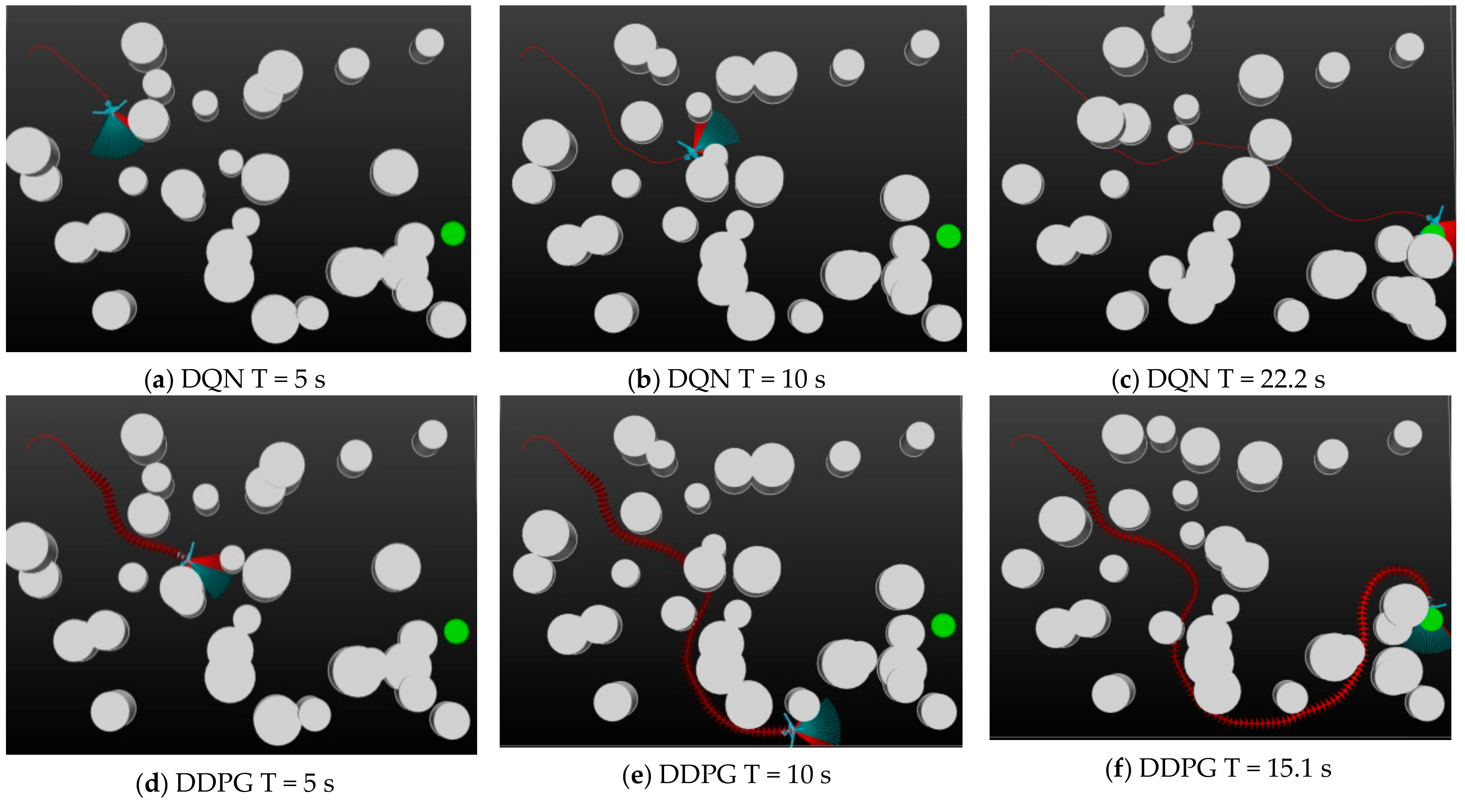
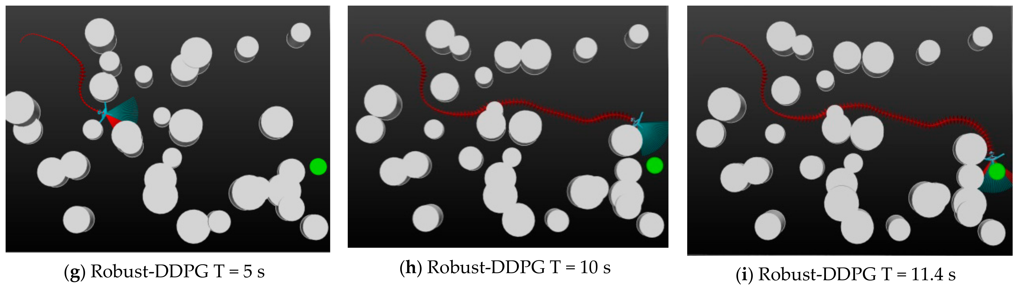
While learning is done, the controller is constructed. In this section, we conduct some UAV exploiting experiments and evaluate the effectiveness of the Robust-DDPG-based controller. Specifically, we let the three controllers constructed by DQN, DDPG, and Robust-DDPG drive a UAV to start from the same initial location (−10, 180), cross the same dynamic environment, and reach the target point (−120, −120). The exploiting environment here is more complicated than the one for learning as Figure 6. We take three screenshots for each controller at T = 5 s, T = 10 s and the terminal time. All the screenshots can be seen in Figure 8.

As we can see in Figure 8, the three controllers fly out completely different trajectories for the same task. DQN flies at a constant speed (20 m/s) and selects a relatively safe path to bypassing the moving threats. At time 22.2 s, it successfully reaches the target and the UAV flies 463.2 m in total. For DDPG, it chooses to avoid intensive threat areas and flies around to maintain safety, which leads to a longer path of 651.1 m. However, by dynamically adjusting the flying speed, it only takes 15.1 s to complete the journey. To clearly show the changing in speed, we use arrows of different sizes to indicate different speeds. Zoom in the pictures in Figure 8 and you will find the difference of the trajectories. Among the three controllers, Robust-DDPG flies the most efficient path. Through fine adjustments in the speed and roll, Robust-DDPG can safely avoid threats and fly quickly to the target. In fact, it only takes 11.4 s and flies 443.5 m to finally finish the task. Obviously, we can conclude that Robust-DDPG provides the most efficient controller, since it enables the UAV to complete the mission with minimum time and path costs. The exploiting effectiveness is intuitively shown in

Table 2. The exploiting effectiveness.

Agent	Flight Time	Path Length
DQN	22.2 s	463.2 m
DDPG	15.1 s	651.1 m
Robust-DDPG	11.4 s	443.5 m

.

4.4. Experiment III: Adaptability of Robust-DDPG

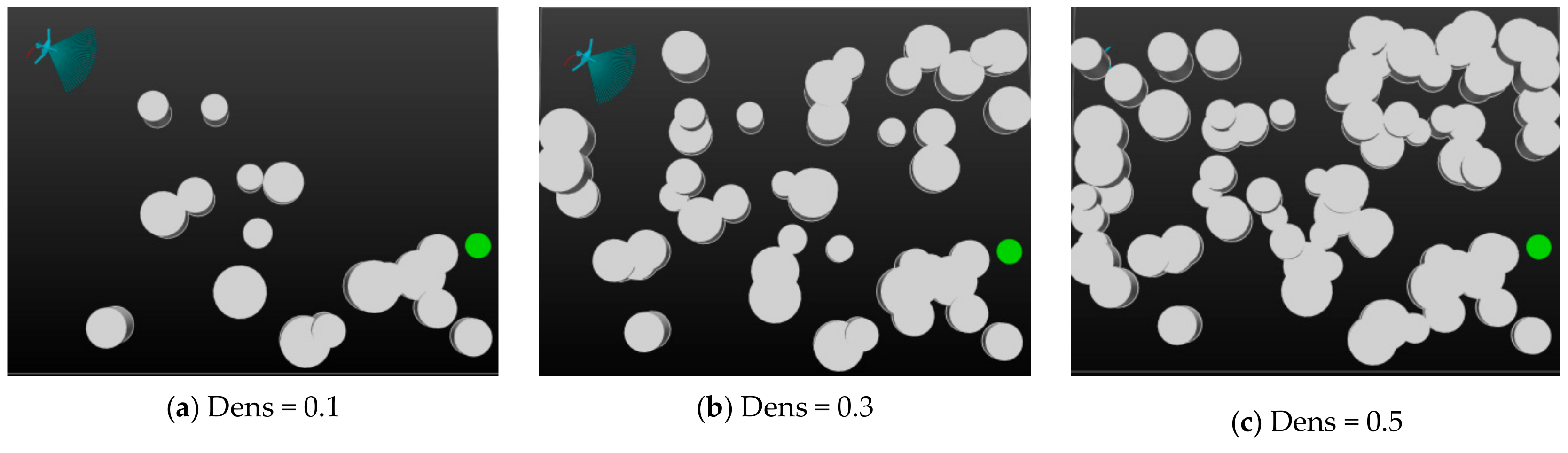
To further validate the Robust-DDPG can be generalized into more complex environments, we conduct a series of other exploiting experiments in this section. The experiments try to perform a comprehensive evaluation of Robust-DDPG’s adaptability to complicated, dynamic, and uncertain environments.

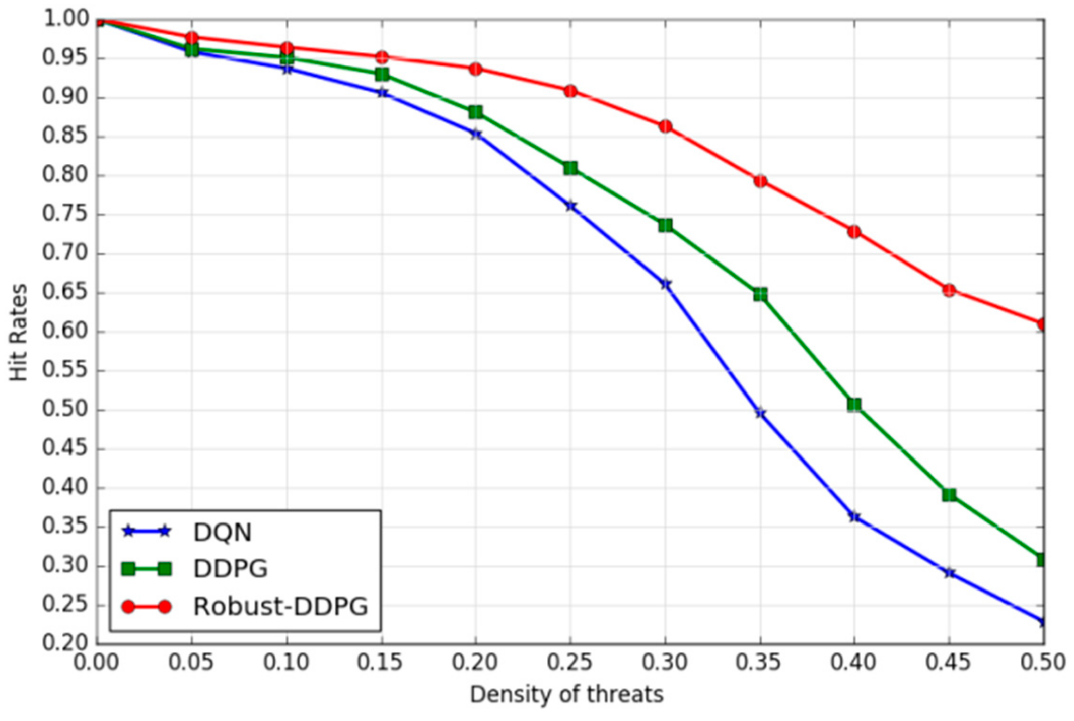
(a) Adaptability to complicated environments: we characterize environmental complexity by the density of threats (Dens). We build a series of environments by increasing the density of threats (Figure 9 illustrates three examples with threat density of 0.1, 0.3 and 0.5) and exploit the three learned agents to drive the UAV to fly in these environments. Each experiment is set to repeat 1000 episodes and each episode randomly re-deploys the UAV and target. The hit rate of the 1000 episodes will be counted after the end of each experiment. Figure 10 depicts the trends of hit rates under different threat densities of the three agents. Obviously, the increasing threat density has caused declines of the hit rates of all the three agents, but Robust-DDPG has presented a slower and smaller decline comparing to DQN and DDPG. In fact, Robust-DDPG has stayed about a hit rate of 61.0% even in a highly complex environment (dens = 0.5), while DQN and DDPG have dropped down to 22.9%, and 30.8%, respectively. In other words, Robust-DDPG shows greatest adaptability to complicated environments.

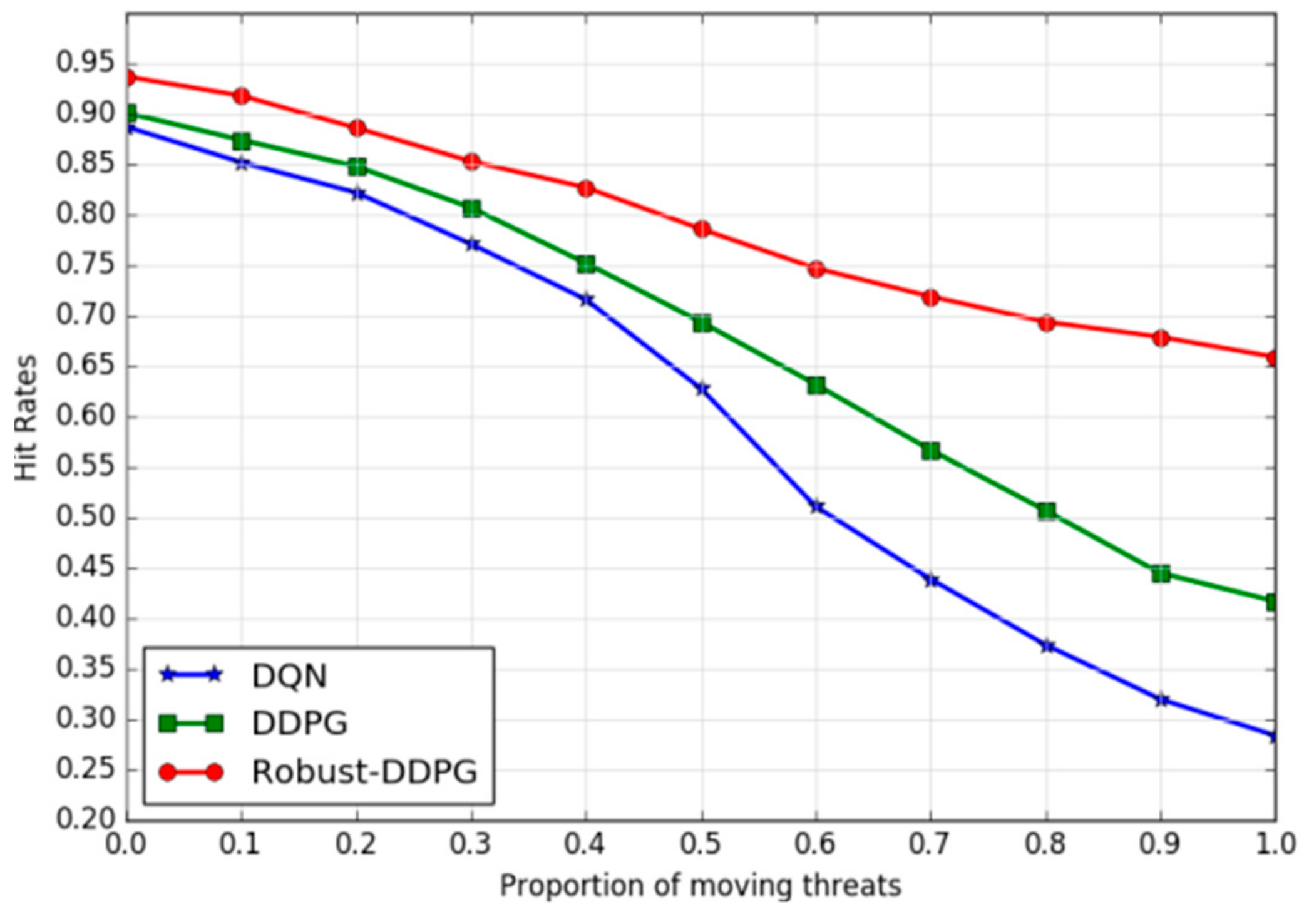
(b) Adaptability to dynamic environments: We use the proportion of moving threats (Pro) among all threats to characterize the dynamics of the environment. Pro = 0 means all the threats are stationary, while Pro = 1 means all of them are movable. The speeds of the moving threats are randomly sampled from a uniform distribution U(5, 10). In the experiments, we gradually increase Pro from 0 to 1 and examine the hit rate trend of the three agents. As illustrated in Figure 11, Robust-DDPG provides better adaptability to dynamic environments. As the proportion of moving threats increases from 0 to 1, Robust-DDPG still reaches a hit rate of nearly 66.0% after a slow decline, while DQN and DDPG dropped rapidly from 88.7% and 90.1% to 28.4% and 41.7%. Robust-DDPG can provide a more stable policy for the UAV control, due to proposed three tricks in this paper.

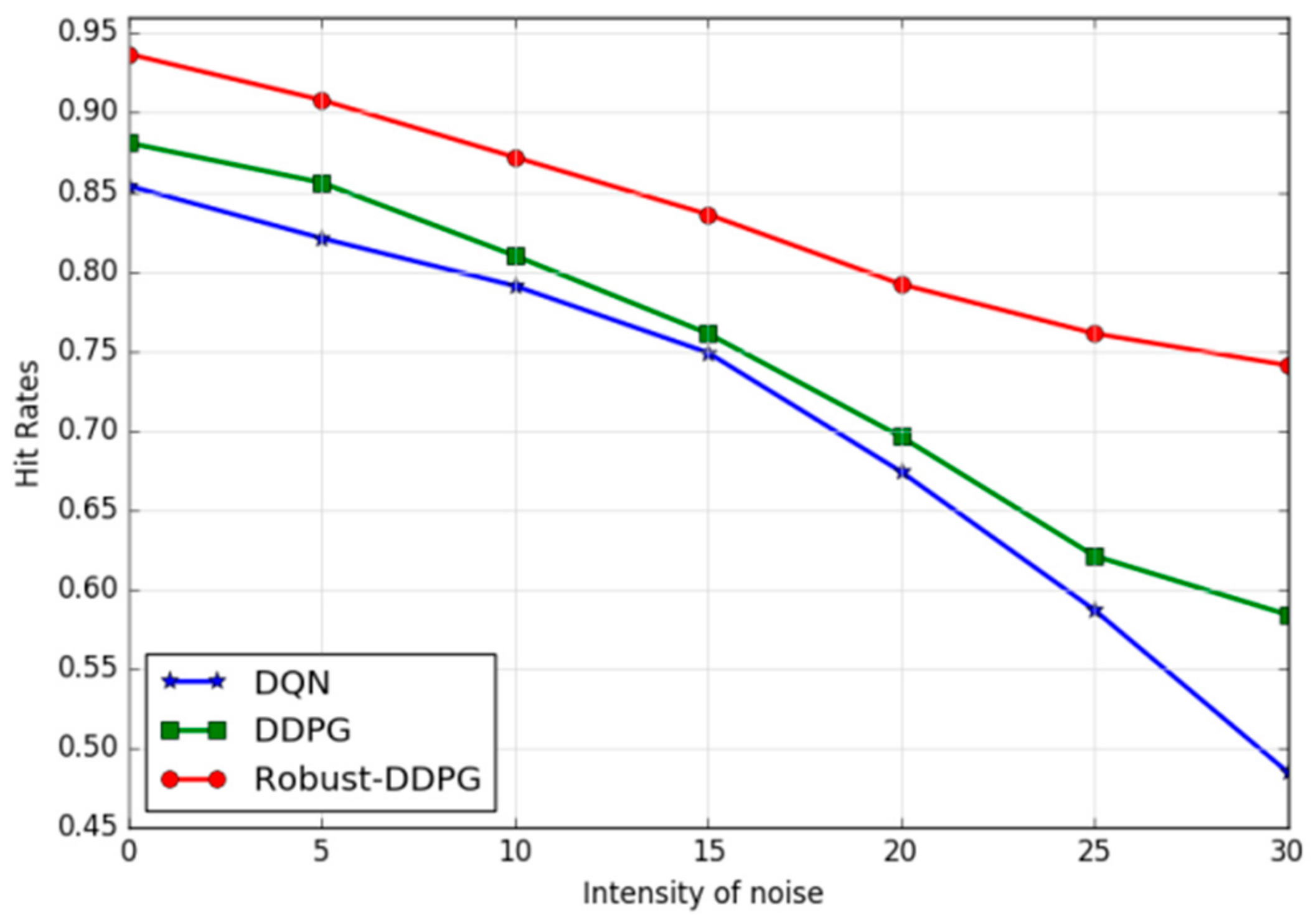
(c) Adaptability to uncertain environments: We increase the uncertainty of the environments by adding noises to the motion of UAV and further explore the Robust-DDPG’s adaptability to these environments. Noise intensity can be represented by disturbances ${\sigma }_{\dot{x}}$ and ${\sigma }_{\dot{y}}$ in Equation (1). So we conduct a series of comparative experiments by gradually increasing the values of ${\sigma }_{\dot{x}}$ and ${\sigma }_{\dot{y}}$, and then evaluate the impact of noise with different intensity on the hit rate. The trends of hit rates under different noise intensities of the three agents are illustrated in Figure 12. As we can see, Robust-DDPG performs great adaptability to uncertain environments, because as ${\sigma }_{\dot{x}}$ and ${\sigma }_{\dot{y}}$ increase from 0 to 30, the hit rate only decreases from 93.7% to 74.1%. This is mainly due to the adversarial attacks during the training process. In contrast, DQN and DDPG present worse robustness to uncertain environments that when the noise intensities increase, larger decreases of the hit rates occur.

5. Discussion

For a comprehensive evaluation of the proposed algorithm, Robust-DDPG, experiments are conducted to verify its training performance, exploiting effectiveness, and environmental adaptability, by comparing it to DQN and DDPG algorithms. Most of the hyper-parameters are tuned by extensive repeated trials and some of them are selected based on domain experience. With respect to the same parameters, three different models are trained and tested in a series of repetitive experiments.

For the training performance evaluation, Robust-DDPG converges to a hit rate of approximate 92.6% in about 2500 episodes, while DQN uses about 5000 episodes to converge to a hit rate of 82.4% and DDPG uses about 4000 episodes to converge to a hit rate of 88.7%. In other words, Robust-DDPG converges to a higher final hit rate with less training time. The great improvements in convergence speed and convergence performance come from the joint work of the mixed exploration trick and the delayed learning trick described in Section 3.2.1 and Section 3.2.3. The former ensures sample diversity in the early learning stage and provide Robust-DDPG more efficient data utilization. The latter keeps the learning in a stable strategic direction and improves the opportunity of learning a better policy.

For the exploiting effectiveness evaluation, the UAV is driven by three controllers to fly from the same departure, across the same dynamic environment, and to the same destination, respectively. The result is Robust-DDPG-based controller flies the most efficient path, that is, the shortest flight time of 11.4 s and the shortest path length of 443.5 m. Comparing the tracks of the three UAVs (in Figure 8), we can see that the control commands provided by Robust-DDPG-based controller perform a better fit between the speed and roll channel. Neither is it as radical as DDPG that flies with high speed and large roll, nor is it as cautious as DQN, which flies with constant low speed and small roll, it just fine-tunes both the speed and roll dynamically according to the sensed environment. This outstanding effectiveness of Robust-DDPG derives from the delayed learning trick. As we described in Section 3.2.1, delayed learning trick ensures the actor and the critic to obey the same principle in an ongoing learning episode and avoids frequent swinging of strategic direction between radical policy and cautious policy. It is a significant trick for learning a reliable policy.

For the environmental adaptability evaluation, there are three sets of experiments. Firstly, we studied the trends of hit rates under different threat densities, and the results clearly show that Robust-DDPG owns better adaptability to complicated environments than DQN and DDPG. As Figure 10 illustrates the smallest decent slop of hit rate for Robust-DDPG. Similarly, the trends of hit rates under different moving threat proportions and the trends of hit rates under different noise intensities are explored, and the results in Figure 11 and Figure 12 leads to the same conclusion, and Robust-DDPG owns better adaptability to dynamic and uncertain environments than DQN and DDPG. Better adaptability means Robust-DDPG can be generalized into more complex environments. This feature is contributed by all the three tricks proposed in this paper, especially the adversarial attack trick. Introducing some adversarial attacks into the training process, the agent learns some additional skills that could be used to handle newly emerged circumstances.

In order to eliminate the impacts of accidental factors, we further carry out some statistical significance tests based on the original data used in Figure 10, Figure 11 and Figure 12. As the data hardly satisfies normality and variance homogeneity, Friedman test is finally used. For simplification, let A, B and C denotes Robust-DDPG, DDPG, and DQN, respectively. To highlight the advantages of Robust-DDPG, we conduct Friedman(A,B), Friedman(A,C), and Friedman(A,B,C) to assess whether the differences between A and B; A and C; A,B and C are really significant. The basic Hypothesis is the difference is not significant. From the test results shown in

Table 3. The Friedman test results.

	P(A,B)	P(A,C)	P(A,B,C)
Data Set 1	0.0016	0.0016	4.5400e-05
Data Set 2	9.1112e-04	9.1112e-04	1.6702e-05
Data Set 3	0.0082	0.0082	9.1188e-04

, we can see that the condition p < 0.05 occurs in all test, which means the Hypothesis has to be rejected. In other words, the differences between Robust-DDPG and DDPG; Robust-DDPG and DQN; Robust-DDPG, DDPG and DQN are all significant. Robust-DDPG does have better adaptability than DDPG and DQN.

From all the experimental results, we conclude that Robust-DDPG performs great advantages in t learning performance, exploiting effectiveness, and environmental adaptability. It is a powerful weapon to provide the UAV great capabilities of autonomous flying in complex environments. However, it is worth mentioning that despite of our efforts in the robustness and adaptation, there are still challenges, while trying to transfer this technique to a real UAV application. In the context of real control, the uncertainty is everywhere and exists all the time, the positioning error, the sensing error, the actuator error or even the crosswind, etc. No matter how well the controller is trained in virtual environment, the reality gap does exist. It is still difficult to figure out in what range of uncertainty the controller can operate safely before adaptation is necessary. It needs some trial and errors with a real UAV. We can characterize as much uncertainty as possible by maintaining insight into flight control system, understand the techniques, and model them in the virtual environment. By constantly reducing the reality gap, we will finally apply this technique in a real UAV platform.

6. Conclusions

This paper presents a learning-based controller to provide the UAV robust motion control in dynamic uncertain environments. The controller is constructed by an actor-critic DRL framework and can be used to perform dual-channel continuous controls of roll and speed. To train a stable controller, an efficient DRL algorithm, Robust-DDPG, is proposed by introducing three critical learning tricks into the original DDPG. A delayed-learning trick is designed to learn a stable policy to adapt to dynamic environments, an adversarial attack trick is adopted to provide enough adaptability to uncertain environments, and a mixed exploration trick is introduced to maintain a faster convergence of the learning. A series of experiments are conducted to evaluate the performance, the effectiveness and the adaptability of the Robust-DDPG from different perspectives. The results show that Robust-DDPG outperforms the state-of-the-art algorithms of DQN and DDPG both in the convergence speed and convergence value. In the exploiting experiments, we conclude that Robust-DDPG can provide a better flying path for the UAV, and provide better adaptability to complicated, dynamic and uncertain environments.

For further research, we plan to extend the UAV motion control problem to a 3D space, which will add a pitch control channel for the UAV. In addition, we intend to construct an intelligent controller for the UAV in an adversarial environment, where the passive threat will be replaced by some aggressive enemies and the UAV will be attacked by these enemies during the whole mission.