Phenological Dynamics Characterization of Alignment Trees with Sentinel-2 Imagery: A Vegetation Indices Time Series Reconstruction Methodology Adapted to Urban Areas


Abstract
1. Introduction
2. Case Study and Data
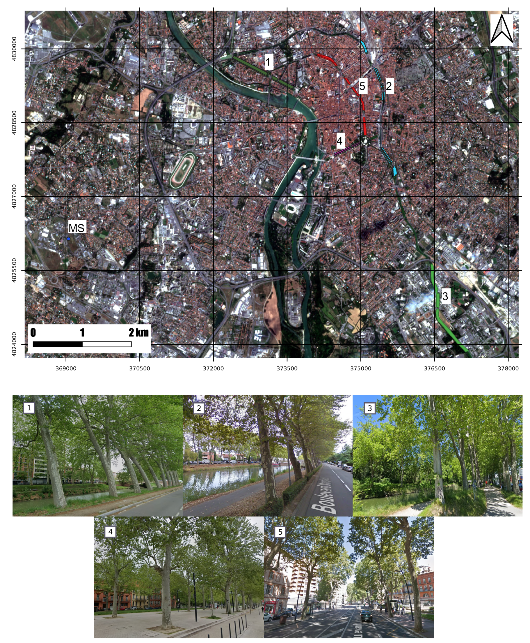
2.1. Case Study
- (1)
- Canal de Brienne (Brienne): These old London planes are located near the city center and grow along a canal. The orientation of this alignment is north-west, with two rows of trees (one at each side of the canal) and crown widths between 10 and 20 m.
- (2)
- Urban Canal de Midi (Midi Int): These London planes grow along a canal inside the city. The orientation of this alignment is mainly north, with two rows of trees (one at each side of the canal) and crown widths between 10 and 20 m.
- (3)
- Peri-urban Canal de Midi (Midi Ext): Located outside the city, the orientation of this alignment presents small variations between north and west. It contains two rows of trees (one at each side of the canal) with crown widths between 10 and 20 m.
- (4)
- Jules Guesde Avenue (JGuesde): Located in Toulouse city center, this alignment is oriented north-east. It contains between two and four rows of trees with crown widths between 5 and 10 m.
- (5)
- Boulevard Francois Verdier-Boulevard Carnot-Boulevard Strasbourg (FVerdier): Located in the city center, the orientation of this alignment presents small variations between north and west. It contains between two and four rows with crown widths of about 10–15 m.
2.2. Sentinel-2 and Meteorological Data: Toulouse (France) 2018
3. Methodology
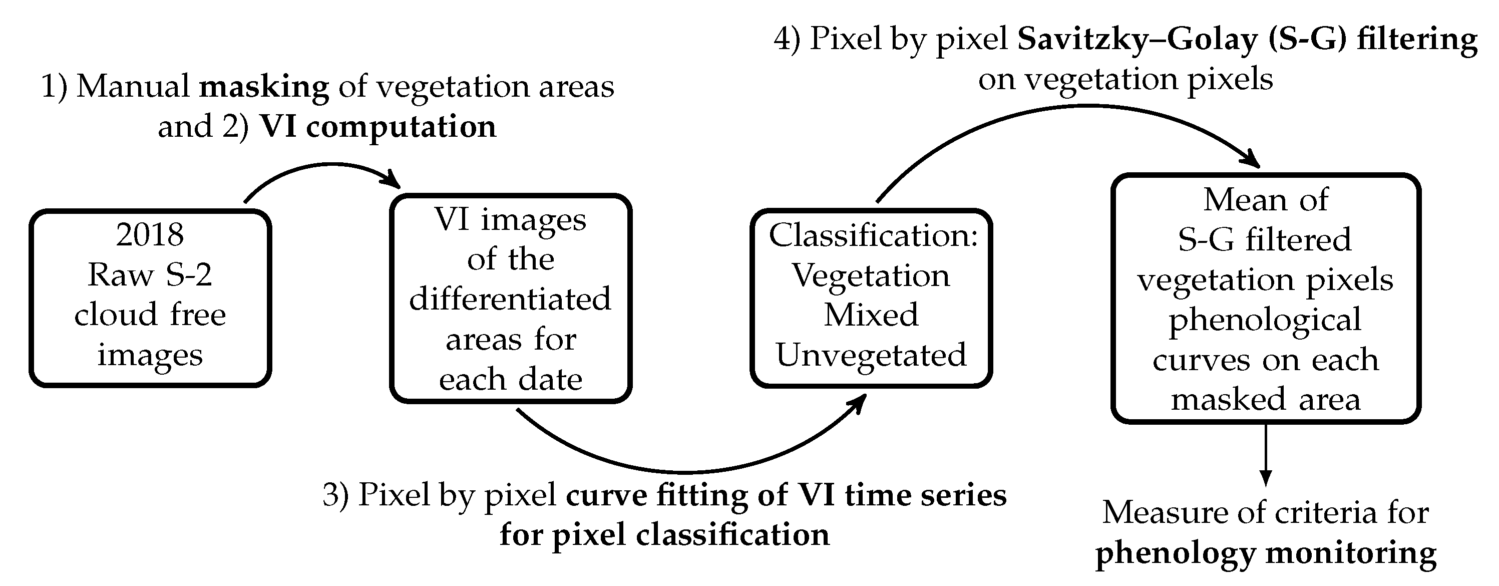
3.1. Phenology Time Series Reconstruction
- (1)
- A manual masking aims at discriminating the vegetation study areas (in this study five masks are created, see Section 2.1). This mask is visually delineated by using S-2 images but also georeferenced open access airborne images of the city (Google Earth images). Only one mask per green studied area was used for the whole studied year. So, to entirely contain the vegetated area, the mask should be set during the period of the year for which vegetation occupies the largest area, both in terms of quantity of pixels and quantity of vegetation per pixel (this period usually corresponds to the maturity period). For this work, QGIS software was used to create the masks.
- (2)
- The chosen VI was calculated for each pixel of the masked areas and for all the available dates of the year. Hence for each pixel, a raw VI time series, , with a number of samples equal to the number of available images, was obtained.
- (3)
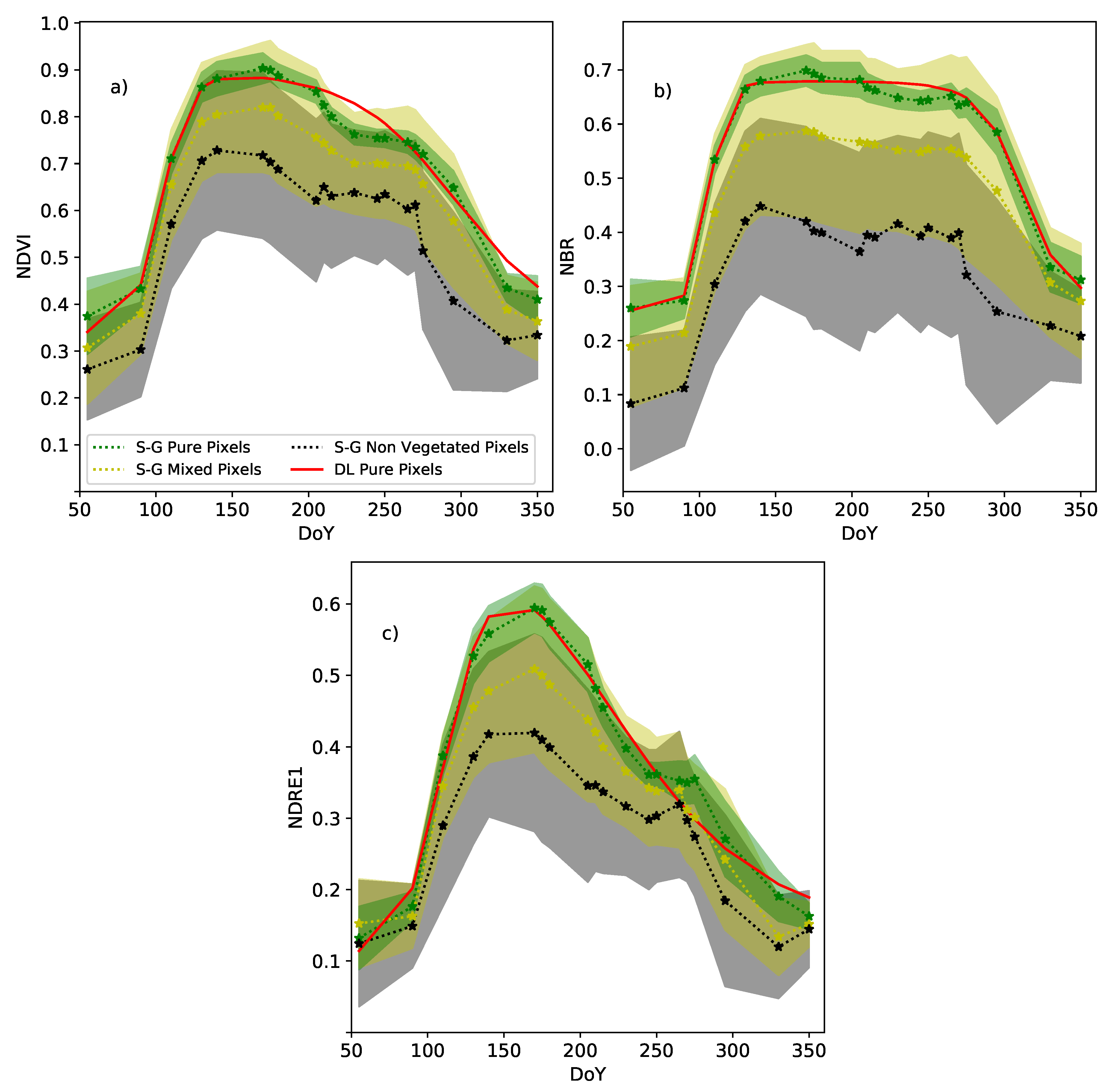
- Then, an unsupervised classification based on pixel by pixel weighted iterative fitting of phenological curves was applied. Weighted iterative curve fitting has been traditionally used to study vegetation phenology, by considering that healthy vegetation presents phenological curves that can be described by fixed functions [45,51,52]. The proposed methodology takes advantage of this hypothesis and considers that pixels where the error fit is large are mixed or non-vegetated pixels. On the other hand, pixels where the error fit is considerably small, i.e., behaving as the imposed function, are considered vegetation pixels. In this work, double logistic function was chosen to describe phenology time series of VIs, since it presents less free parameters than the double hyperbolic tangent function and it has been shown to perform better than the asymmetric Gaussian function [51]. The double logistic function is expressed as:where , , S, A, and are the free parameters of the fit. With the minimum yearly value of the VI, its maximum yearly value, S the Day of the Year (DoY) indicating the inflection point when the curve raises (greenup period), A the DoY indicating the inflection point when the curve drops (senescence period) and and the slopes of the curve at days S and A respectively.The weighted iterative process relies on the hypothesis that in urban environments, small co-registration errors between dates are the main source of noise induced on time series, and thus, considers that sudden increases or drops of values between dates are mainly due to changes in the fraction of vegetation within a pixel. To correctly characterize the vegetation phenology and reduce mixed pixels effect, more weight should be given to high VI values.Then from a first fit () of the pixel raw time series (), a set of weights are computed to give more prominence to high VIs values than to low ones (upper envelope of the curve):where is the weight of sample at date , is the raw VI time series, is the first fitted VI time series, and .Once the weights have been fixed from the first fitting, an iterative process starts until minimizing the fitting error defined as:where is the error at iteration k and N is the number of samples in the time series. Fits are performed with the Levenberg–Marquardt least squares method [72,73] of the SciPy library [74] for Python 3.6.Finally, pixel classification is based on errors and two thresholds, and . If then the pixel is considered as vegetated, if the pixel is considered as mixed and if the pixel is considered as not (or poorly) vegetated. and were empirically chosen to be respectively 5% and 10% of the annual maximal value VI of the pixel. For our study case, these bounds appear strict enough to importantly reduce non-vegetated pixels in those classified as vegetation. An additional condition was applied: among the pixels initially classified as vegetation on each masked area, only pixels whose mean VI value during the maturity period is comprised within one standard deviation (std) of the ensemble of vegetation pixels over the same period, were retained. For London planes in Toulouse, we defined this period between 1st of May and 1st of October, since for this species in Toulouse, greenup and senescence periods correspond to the beginning of spring and the beginning of autumn respectively. Background effects are major during winter (when there are no leaves) and during the start of the greenup period and the end of the senescence period. So, the choice of the maturity period bounds were done considering that from 1st of May to 1st of October the vegetation cover should be enough to minimize the influences of ground in the statistical measures. Adding this condition on the mean VI values allows us to avoid, as much as possible, false-positives in the classification.
- (4)
- A weighted iterative Savitzky–Golay filtering was applied on vegetation pixels as classified in step (3). It allows us to reduce the noise that registration variability between dates induces on time series, and as it does not fix the phenological behavior, it allows us to observe intra-annual periods of disturbance and anomalies in vegetation phenological curves. The weighted iterative Savitzky–Golay filter used in this work is our own implementation (in Python 3.6) of the filter presented in Chen et al. 2004 [50], but it was adapted to process not uniformly sampled time series. Savitzky–Golay filter presents two free parameters: the width of the smoothing window (m) and the degree of the fitting polynomial (d).
- (a)
- First, an automatic search of the best parameter values within a given range, and , was done [50]. These ranges were fixed following [50] and considering the number of available dates. On one hand, too small m values may lead to an over-fit of the raw VI time series, and so, difficulties can raise in capturing long-term trends. However, too large m values may lead to neglecting some important variations in the phenological curve. On the other hand, small values of d may lead to smoother results, and large values of d may over-fit the raw VI time series and generate noisy results. In addition, to perform a polynomial fit, the degree d of the polynomial must be lower than the size m of the smoothing window.
- (b)
- Then, once the first filtering was performed providing , weights were assigned following the same hypothesis as in Equation (2), and a new VI time series () is:where “filt” indicates filtered signal, and “ts” indicates built VI time series.
- (c)
- Savitzky–Golay is applied iteratively on the new obtained VI time series () with smaller smoothing window size () and greater polynomial order (). The iterative process searches at minimizing the error defined such as in Equation (3).
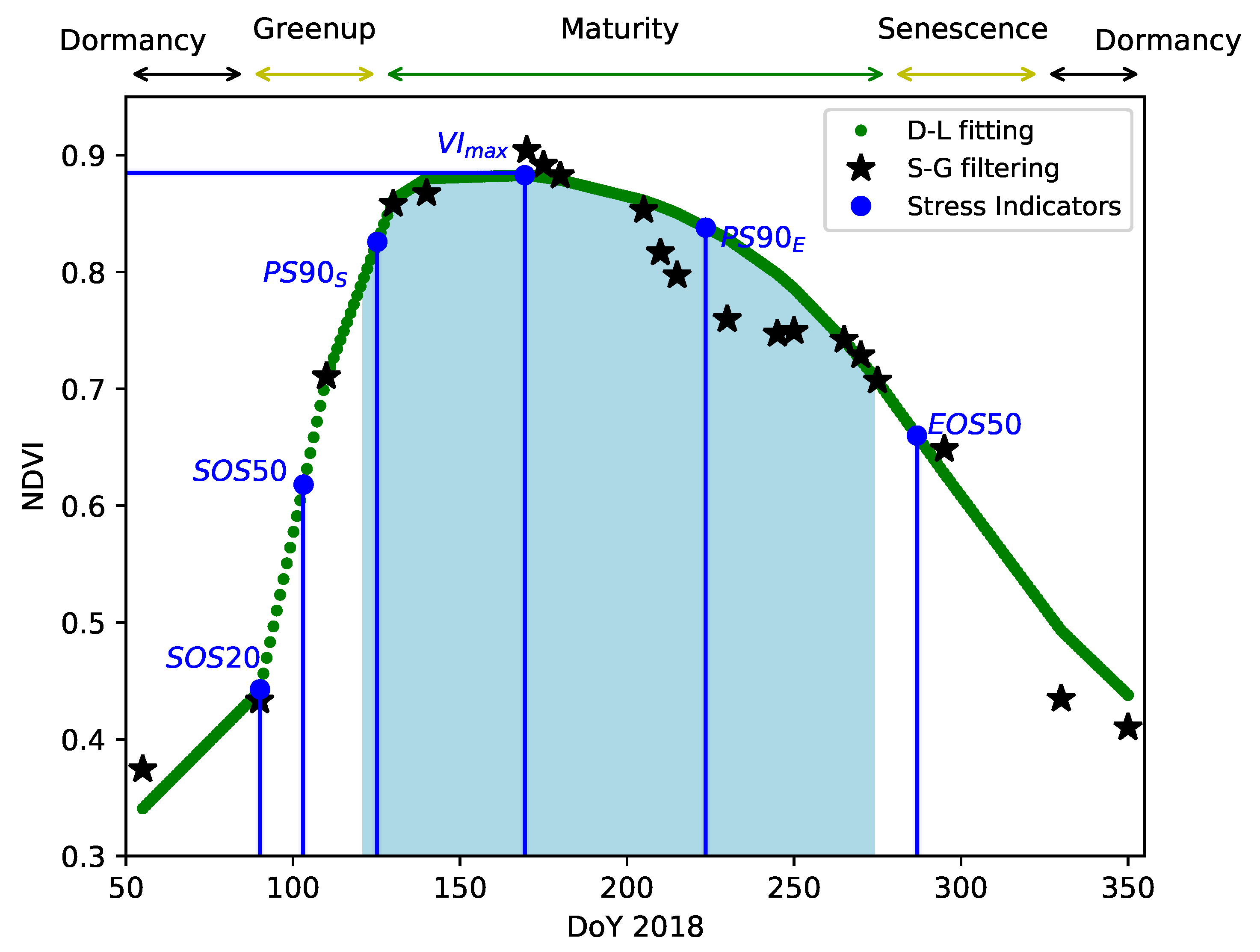
3.2. Annual Phenology Characterization
- (a)
- : The maximum value of the VI reached during the year, see Figure 4.
- (b)
- Greenperiod: Normalized area under the curve during the maturity period (defined from 1st of May to 1st of October), see Figure 4. Measured areas are normalized with respect to the maximal possible VI area in this period. For normalized VIs (such as NDVI, NDRE1 and NBR), the maximal possible area is equal to the area under the unity-valued square-shaped function between 1st of May and 1st of October. Thus, the measure is equivalent to a mean VI value for the maturity period.
- (c)
- SOS20 (Start Of Season), SOS50, PS90 (Peak Season): Days of the year at which the VI amplitude is, respectively, 20%, 50% and 90% of the maximum amplitude, during the spring/summer period, i.e., the greenup period, see Figure 4.
- (d)
- EOS20 (End Of Season), EOS50, PS90: Days of the year at which the VI amplitude is, respectively, 20%, 50% and 90% of the maximum amplitude, during the summer/fall period, i.e., the vegetation senescence period, see Figure 4.
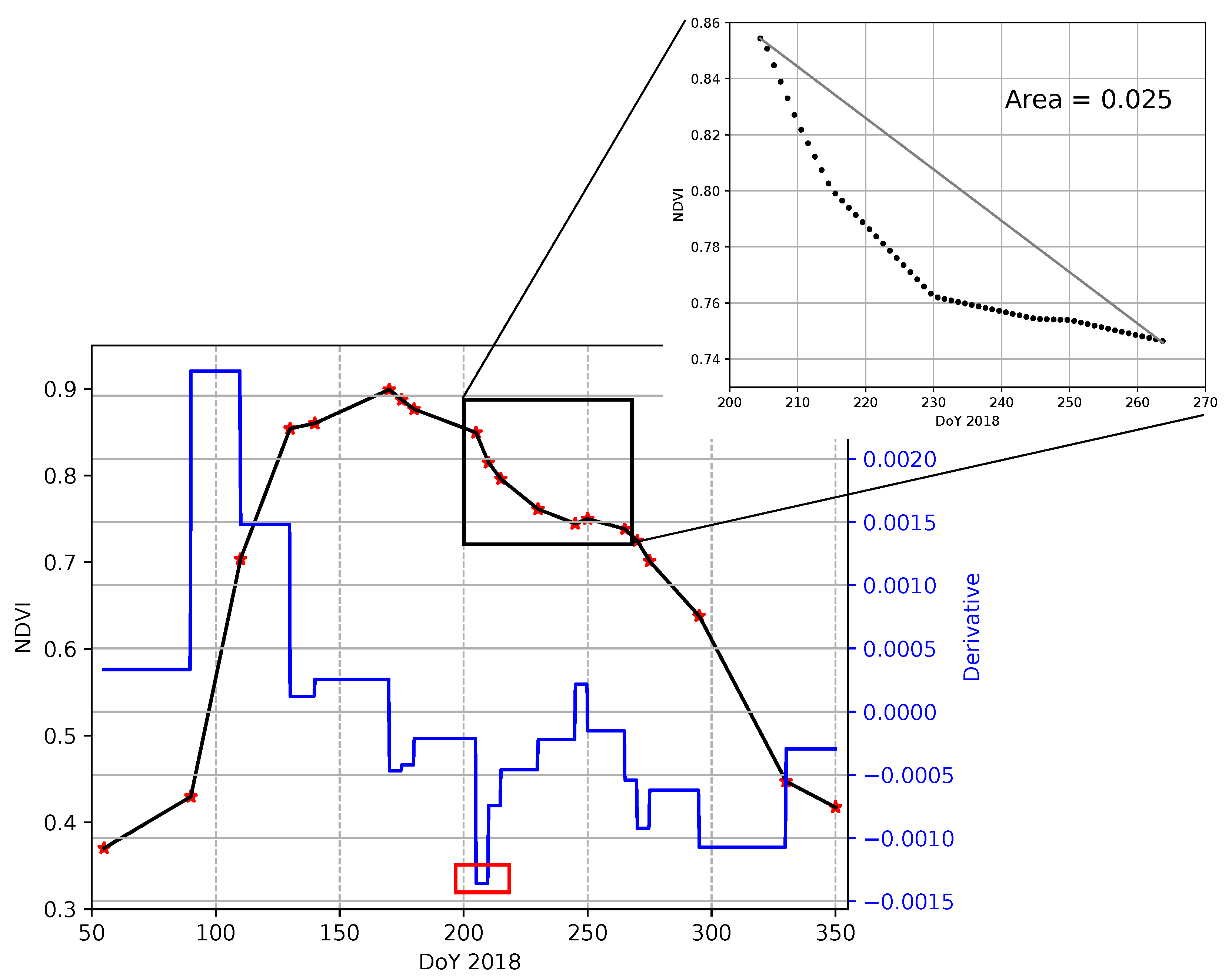
3.3. Intra-Annual Phenology Characterization
- (e)
- SlVI: Negative slope (VI/day) of the VI curve at the beginning of the phenological disturbance period, see Figure 5. This indicator provides information on the strength of the perturbation. The more negative the slope is, the more important the phenological disturbance is, i.e., the more important is the concavity break.
- (f)
- DiffA: Normalized area between the phenological curve and the straight line joining the start and the end of the phenological disturbance period, see Figure 5. Normalization is applied over the number of days corresponding to the phenological disturbance period. This straight line is assumed to be the lower possible bound of a non-disturbed phenological curve. This indicator not only provides information on the importance of the perturbation but also on the capacity of the vegetation to restore.
4. Results
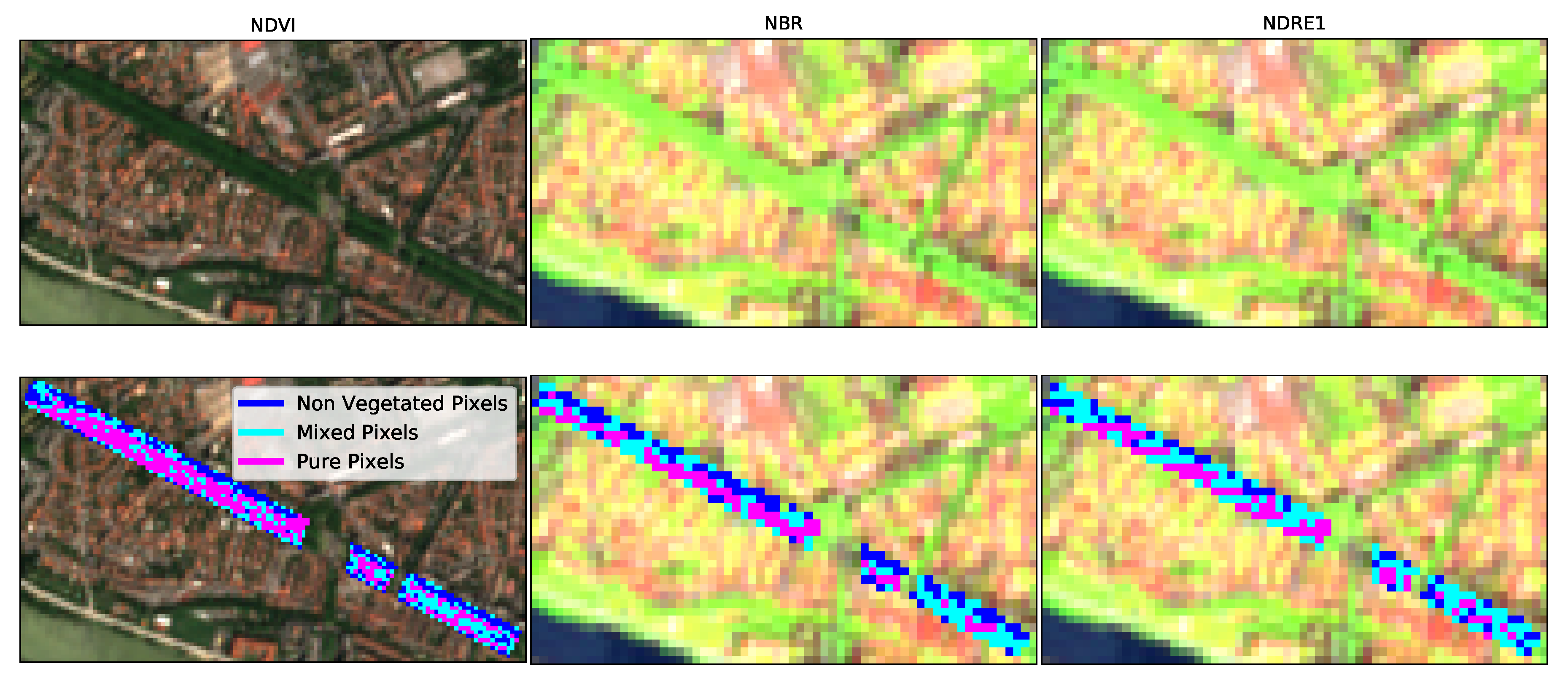
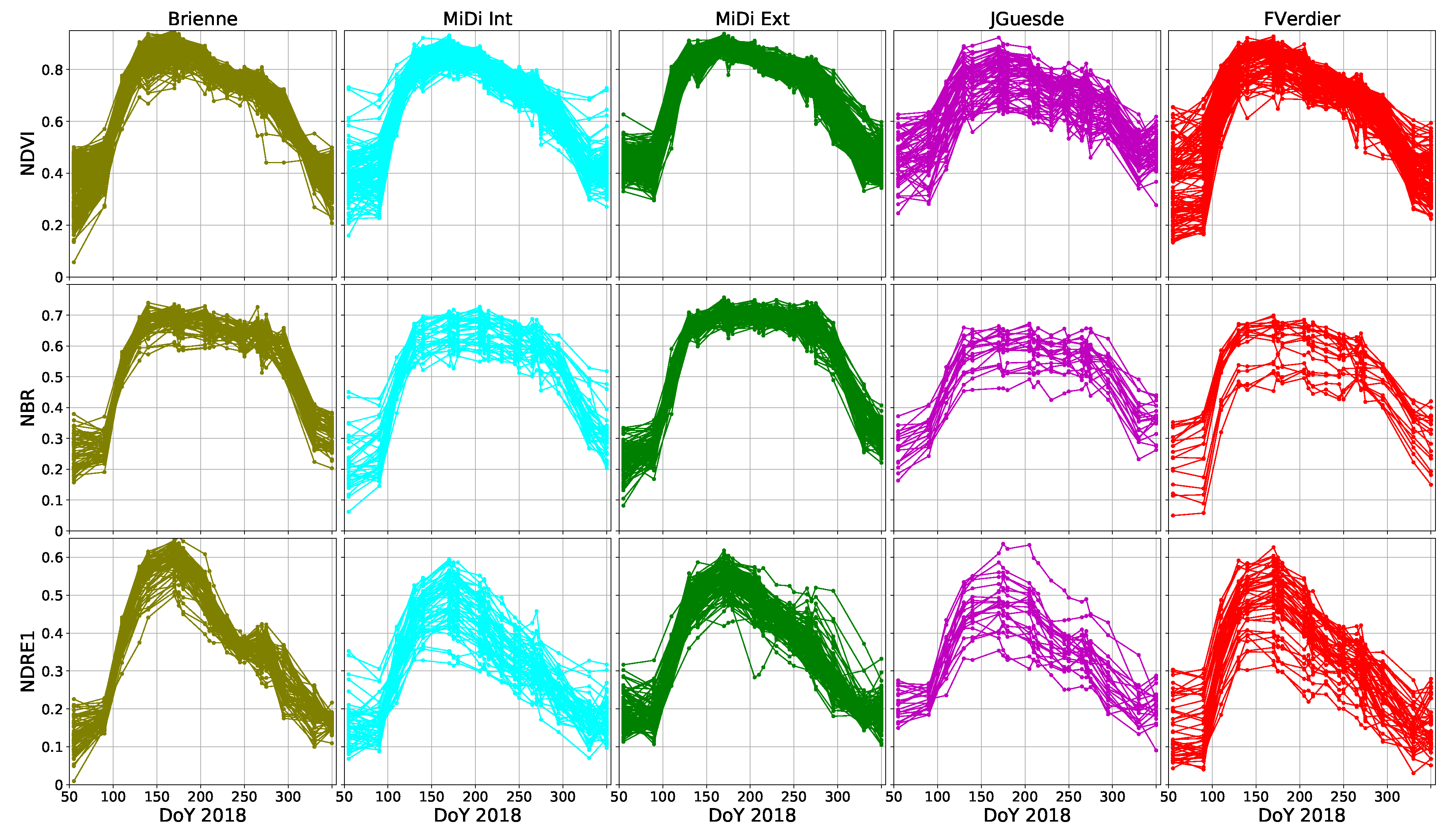
4.1. Classification of Vegetation Pixels
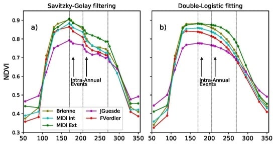
4.2. Savitzky–Golay Filtering to Build Vi Time Series
4.3. Analysis of Phenological Dynamics from Vi Time Series
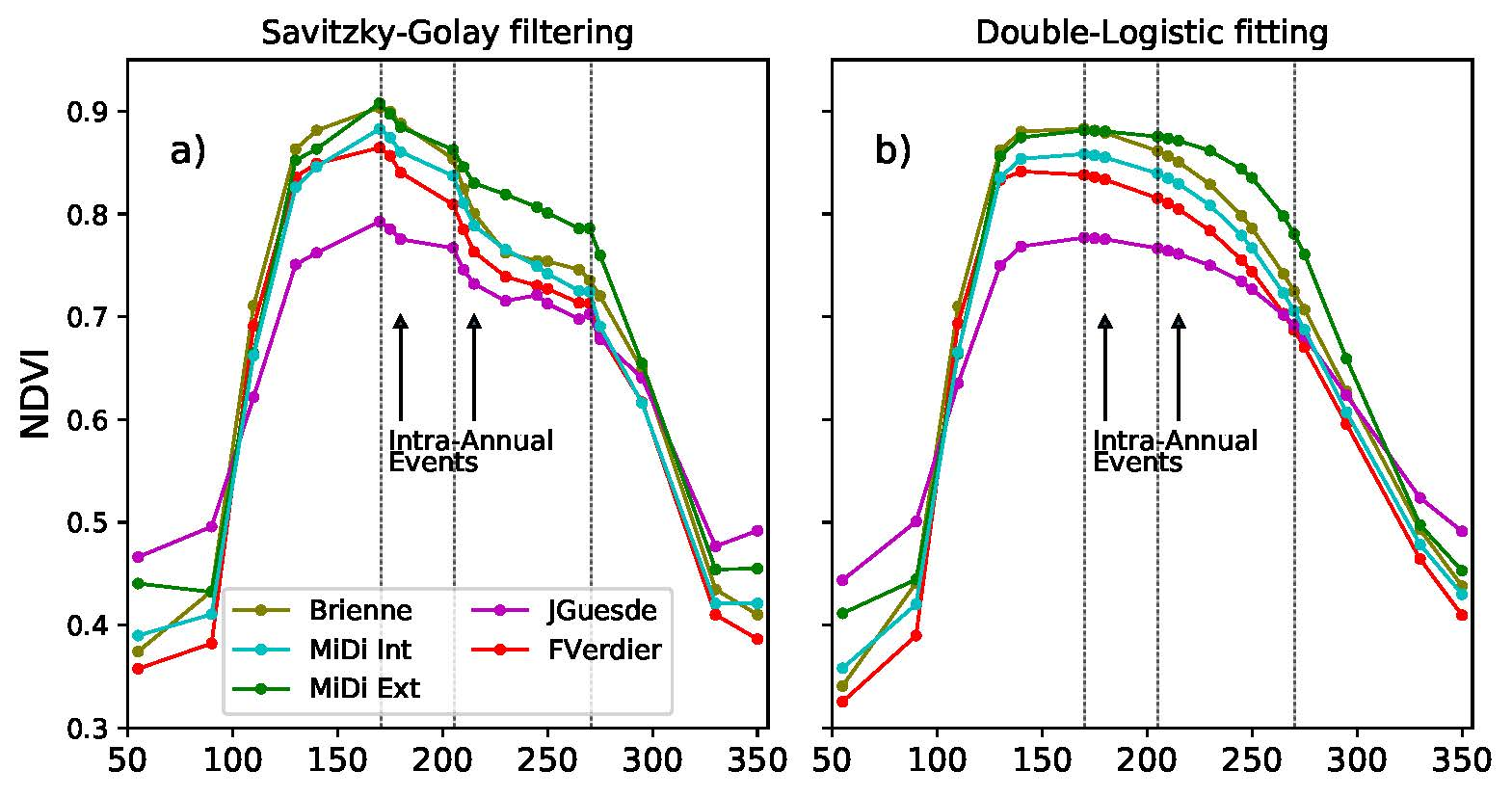
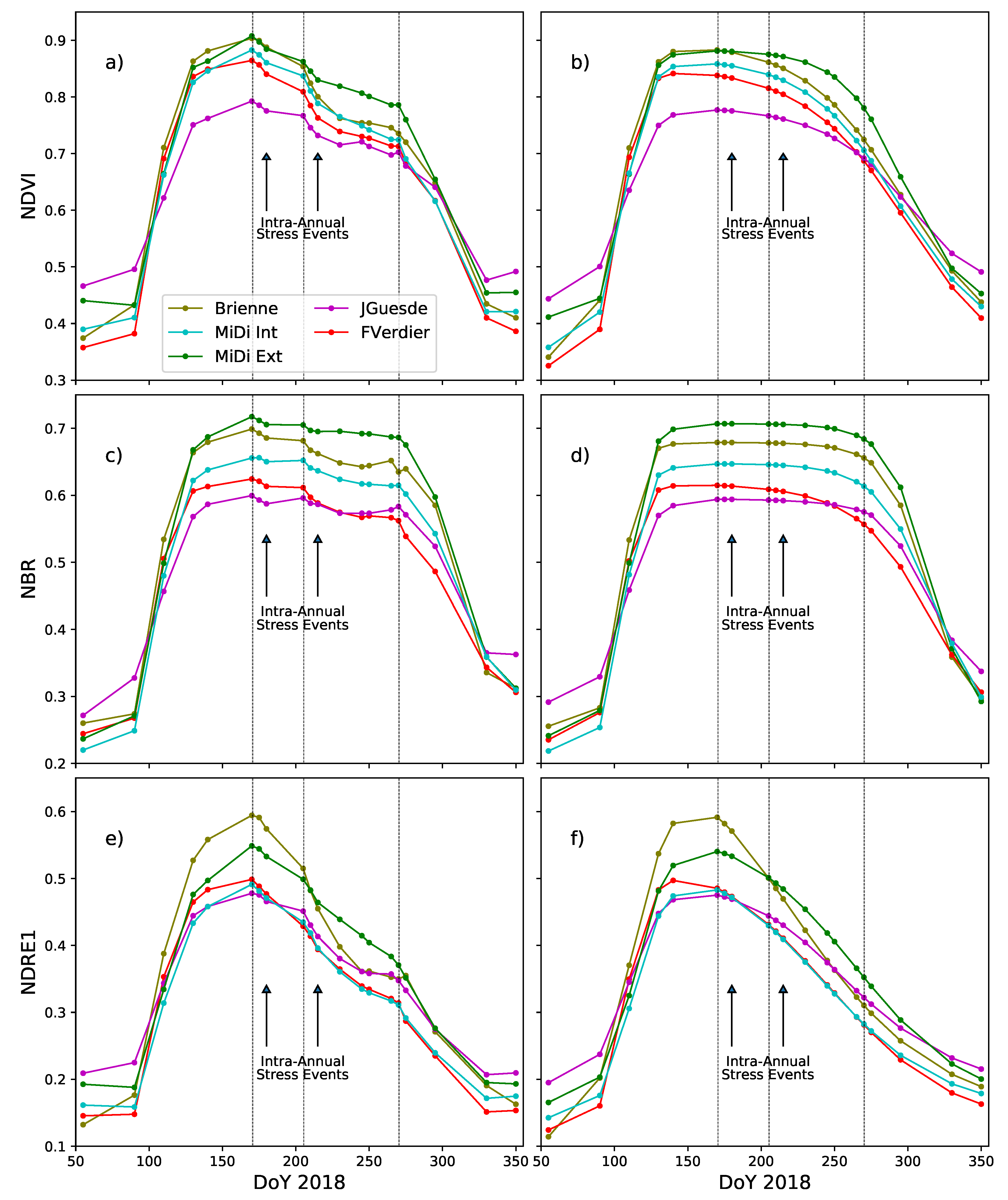
4.3.1. Annual Dynamics
4.3.2. Intra-Annual Phenological Disturbance Events Analysis
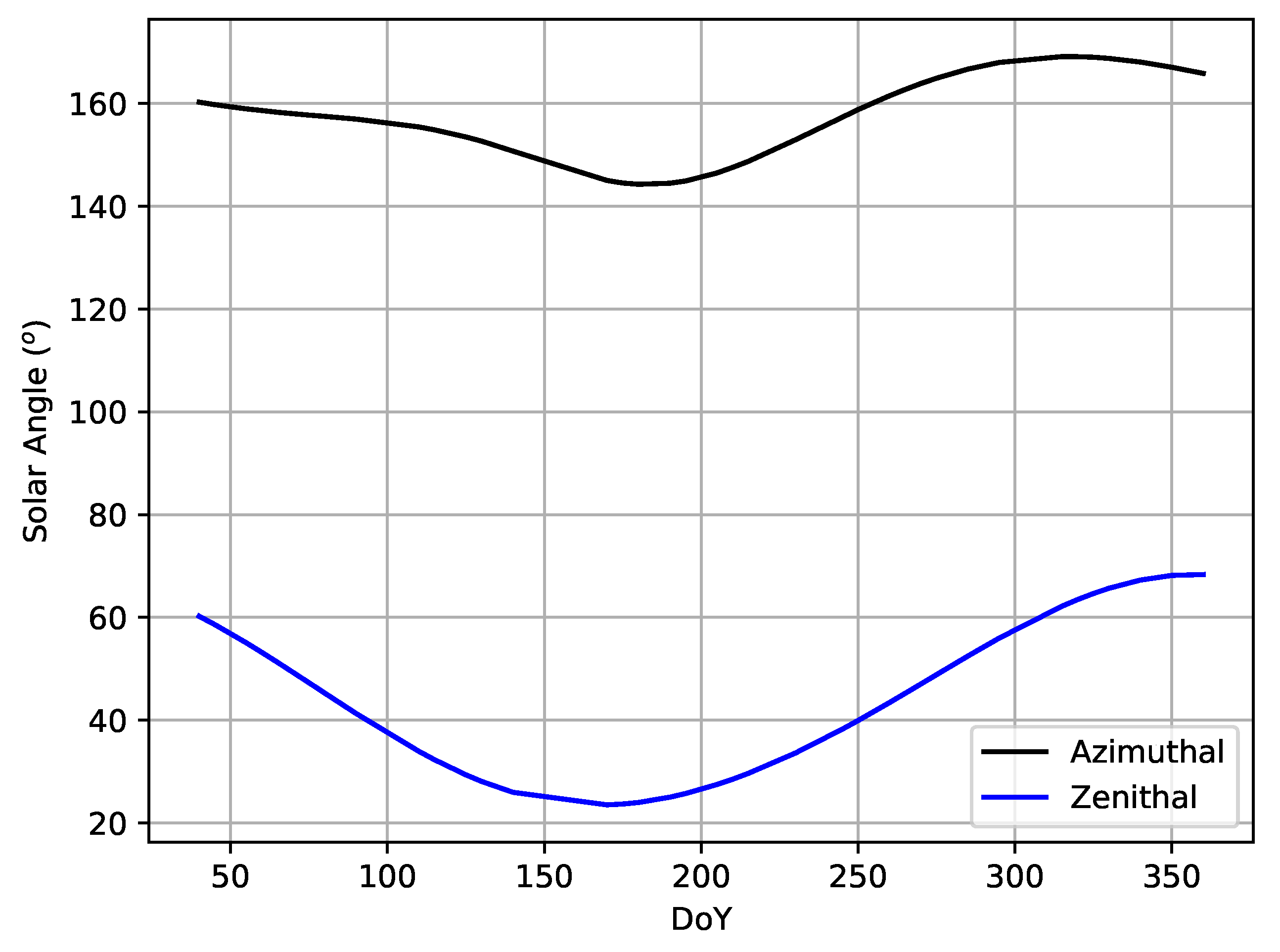
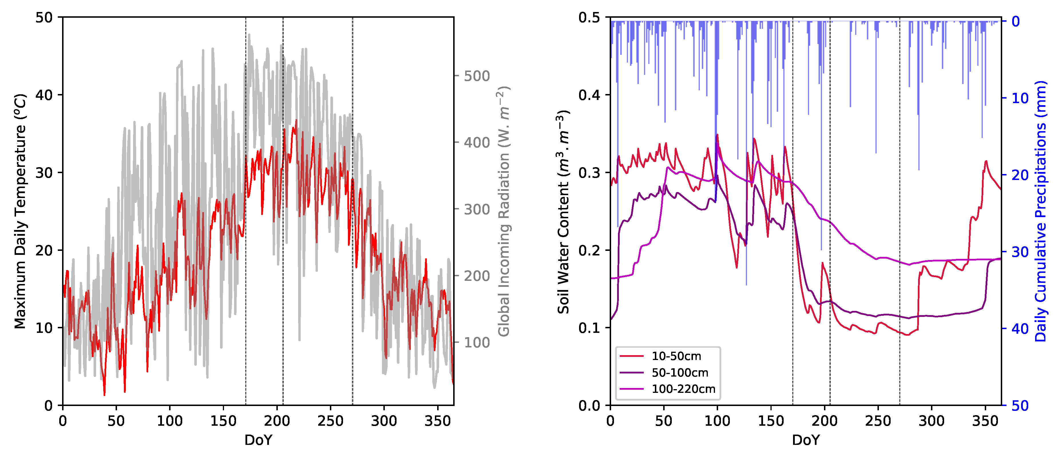
4.4. Climate Factor Influences on Phenological Curves
5. Discussion
5.1. Methodology Hypotheses and Performances
5.2. Vegetation Phenology Characterization
5.3. Meteorological Influences on Intra-Annual Phenological Dynamics
6. Conclusions
Author Contributions
Funding
Acknowledgments
Conflicts of Interest
Appendix A. Sentinel-2 Spectral and Spatial Configuration

| Sentinel-2 Band | Wavelength | Spatial Resolution |
|---|---|---|
| Band 1 - Blue 1 | 433–453 nm | 60 m |
| Band 2 - Blue 2 | 458–523 nm | 10 m |
| Band 3 - Green | 543–578 nm | |
| Band 4 - Red 1 | 650–680 nm | |
| Band 5 - Red 2 | 698–713 nm | 20 m |
| Band 6 - Red 3 | 733–748 nm | |
| Band 7 - Red 4 | 773-793 nm | |
| Band 8 - NIR 1 | 785–900 nm | 10 m |
| Band 8a - NIR 2 | 855–875 nm | 20 m |
| Band 9 - NIR 3 | 935–955 nm | 60 m |
| Band 10 - CIRRUS | 1360–1390 nm | |
| Band 11 - SWIR 1 | 1565–1655 nm | 20 m |
| Band 12 - SWIR 2 | 2100–2280 nm |
References
- Hassan, A.; Lee, H. Toward the sustainable development of urban areas: An overview of global trends in trials and policies. Land Use Policy 2015, 48, 199–212. [Google Scholar] [CrossRef]
- Manning, W. Plants in urban ecosystems: Essential role of urban forests in urban metabolism and succession toward sustainability. Int. J. Sustain. Dev. World Ecol. 2008, 15, 362–370. [Google Scholar] [CrossRef]
- Alexandre, F. The role of vegetation in the urban policies of european cities in the age of the sustainable city. Eur. Spat. Res. Policy 2013, 20, 11–26. [Google Scholar] [CrossRef]
- Vos, P.; Maiheu, B.; Vankerkom, J.; Janssen, S. Improving local air quality in cities: To tree or not to tree? Environ. Pollut. 2013, 183, 113–122. [Google Scholar] [CrossRef] [PubMed]
- Alavipanah, S.; Wegmann, M.; Qureshi, S.; Weng, Q.; Koellner, T. The role of vegetation in mitigating urban land surface temperatures: A case study of Munich, Germany during the warm season. Sustainability 2015, 7, 4689–4706. [Google Scholar] [CrossRef]
- Chaturvedi, A.; Kamble, R.; Patil, N.; Chatuverdi, A. City-forest relationship in Nagpur: One of the greenest cities of India. Urban Ofrestry Urban Green. 2013, 12, 79–87. [Google Scholar] [CrossRef]
- Salbitano, F.; Borelli, S.; Conigliaro, M.; Chen, Y. Guidelines on Urban and Peri-Urban Forestry; Technical report; Food and Agricultural Organization of the United Nations: Rome, Italy, 2016; pp. 1–172. [Google Scholar]
- McPherson, E.G.; van Doorn, N.; de Goede, J. Structure, function and value of street trees in California, USA. Urban For. Urban Green. 2016, 17, 104–115. [Google Scholar] [CrossRef]
- Rol-Tanguy, F.; Alba, D.; Dragoni, M.; Minassian, H.T.; Blancot, C. Essai de Bilan sur le Developpement des Arbres D’Alignement dans Paris; Technical report; Atelier Parisien d’Urbanisme (APUR): Paris, France, 2010; pp. 1–76. [Google Scholar]
- Grimm, N.; Faeth, S.; Golubiewski, N.; Redman, C.; Wu, J.; Bai, X.; Briggs, J. Global change and the ecology of cities. Science 2008, 319, 756–760. [Google Scholar] [CrossRef]
- Salinitro, M.; Alessandrini, A.; Zappi, A.; Tassoni, A. Impact of climate change and urban development on the flora of a southern European city: Analysis of biodiversity change over a 120-year period. Sci. Rep. 2019, 9, 9464. [Google Scholar] [CrossRef]
- Nowak, D. Improving city forests through assessment, modelling and monitoring. Unasylva 2018, 69, 30–36. [Google Scholar]
- Cumming, A.; Galvin, M.; Rabaglia, M.; Cumming, J.; Twardus, D. Forest health monitoring protocol applied to roadside trees in Maryland. J. Arboric. 2001, 27, 126–138. [Google Scholar]
- Ouerghemmi, W.; Gadal, S.; Mozgeris, G. Urban vegetation mapping using hyperspectral imagery and spectral library. In Proceedings of the IEEE International Geoscience and Remote Sensing Symposium (IGARSS), Valencia, Spain, 23–27 July 2018; pp. 1632–1635. [Google Scholar]
- Feng, Q.; Liu, J.; Gong, J. UAV remote sensing for urban vegetation mapping using random forest and texture analysis. Remote Sens. 2015, 7, 1074–1094. [Google Scholar] [CrossRef]
- Hashim, H.; Latif, Z.A.; Adnan, N.A. Urban vegetation classification with NDVI thresold value method with very high resolution (VHR) PLEIADES Imagery. Int. Arch. Photogramm. Remote Sens. Spat. Inf. Sci. 2019, XLII-4, 237–240. [Google Scholar] [CrossRef]
- Mathieu, R.; Aryal, J.; Chong, A. Object-based classification of Ikonos imagery for mapping large-scale vegetation communities in urban areas. Sensors 2007, 7, 2860–2880. [Google Scholar] [CrossRef]
- Tigges, J.; Lakes, T.; Hostert, P. Urban vegetation classification: Benefits of multitemporal RapidEye satellite data. Remote Sens. Environ. 2013, 136, 66–75. [Google Scholar] [CrossRef]
- Wen, D.; Huang, X.; Liu, H.; Liao, W.; Zhang, L. Semantic classification of urban trees using very high resolution satellite imagery. IEEE J. Sel. Top. Appl. Earth Obs. Remote Sens. 2017, 10, 1413–1424. [Google Scholar] [CrossRef]
- Degerickx, J.; Roberts, D.; McFadden, J.; Hermy, M.; Somers, B. Urban tree health assessment using airborne hyperspectral and LiDAR imagery. Int. J. Appl. Earth Obs. Geoinf. 2018, 73, 26–38. [Google Scholar] [CrossRef]
- Sari, N.; Kushardono, D. Quality analysis of single tree object with obia and vegetation index from lapan surveillance aircraft multispectral data in urban area. Geoplan. J. Geomat. Plan. 2016, 3, 93–106. [Google Scholar] [CrossRef][Green Version]
- Xiao, Q.; McPherson, E. Tree health mapping with multispectral remote sensing data at UC Davis, California. Urban Ecosyst. 2005, 8, 349–361. [Google Scholar] [CrossRef]
- Cârlan, I.; Mihai, B.A.; Nistor, C.; GroBe-Stoltenberg, A. Identifying urban vegetation stress factors based on open access remote sensing imagery and field observations. Ecol. Inform. 2020, 55, 101032. [Google Scholar] [CrossRef]
- Li, Y.; Yu, H.; Wang, Y.; Wu, J.; Yang, L. Classification of urban vegetation based on unmanned aerial vehicle reconstruction point cloud and image. Remote Sens. Land Resour. 2019, 31, 149–155. [Google Scholar]
- Jarocińska, A.; Bialczak, M.; Slawik, L. Application of aerial hyperspectral images in monitoring tree biophysical parameters in urban areas. Misc. Geogr. 2018, 22, 56–62. [Google Scholar] [CrossRef]
- Delegido, J.; Wittenberghe, S.V.; Verrelst, J.; Ortiz, V.; Veroustraete, F.; Valcke, R.; Samson, R.; Rivera, J.P.; Tenjo, C.; Moreno, J. Chlorophyll content mapping of urban vegetation in the city of Valencia based on the hyperspectral NAOC index. Ecol. Indic. 2014, 40, 34–42. [Google Scholar] [CrossRef]
- Jensen, R.; Hardin, P.; Bekker, M.; Farnes, D.; Lulla, V.; Hardin, A. Modeling urban leaf area index with AISA+ hyperspectral data. Appl. Geogr. 2009, 29, 320–332. [Google Scholar] [CrossRef]
- Zhang, W.; Zhang, X.; Li, L.; Zhang, Z. Urban forest in Jinan city: Distribution, classification and ecological significance. Catena 2007, 69, 44–50. [Google Scholar] [CrossRef]
- Zhang, X.; Friedl, M.A.; Schaaf, C.B.; Strahler, A.H.; Hodges, J.C.F.; Gao, F.; Reed, B.C.; Huete, A. Monitoring vegetation phenology using MODIS. Remote Sens. Environ. 2003, 84, 471–475. [Google Scholar] [CrossRef]
- Seyednasrollah, B.; Young, A.; Hufkens, K.; Milliman, T.; Friedl, M.; Frolking, S.; Richardson, A. Tracking vegetation phenology across diverse biomes using version 2.0 of the PhenoCam Dataset. Sci. Data 2019, 6, 222. [Google Scholar] [CrossRef]
- Lu, H.; Raupach, M.; McVicar, T.; Barret, D. Decomposition of vegetation cover into woody and herbaceous components using AVHRR NDVI time series. Remote Sens. Environ. 2003, 86, 1–18. [Google Scholar] [CrossRef]
- Hill, M.; Donald, G. Estimating spatio-temporal patterns of agricultural productivity in fragmented landscapes using AVHRR NDVI time series. Remote Sens. Environ. 2003, 84, 367–384. [Google Scholar] [CrossRef]
- Jacquin, A.; Sheeren, D.; Lacombe, J.P. Vegetation cover degradation assessment in Madagascar savanna based on trend analysis of MODIS NDVI time series. Int. J. Appl. Earth Obs. Geoinf. 2010, 12, S3–S10. [Google Scholar] [CrossRef]
- Eckert, S.; Husler, F.; Liniger, H.; Hodel, E. Trend analysis of MODIS NDVI time series for detecting land degradation and regeneration in Mongolia. J. Arid. Environ. 2015, 113, 16–28. [Google Scholar] [CrossRef]
- Liu, Y.; Hill, M.; Zhang, X.; Wang, Z.; Richardson, A.; Hufkens, K.; Filippa, G.; Baldocchi, D.D.; Ma, S.; Verfaillie, J.; et al. Using data from Landsat, MODIS, VIIRS and PhenoCams to monitor the phenology of California oak/grass savanna and open grassland across spatial scales. Agric. For. Meteorol. 2017, 237–238, 311–325. [Google Scholar] [CrossRef]
- Vrieling, A.; Skidmore, A.K.; Wang, T.; Meroni, M.; Ens, B.J.; Oosterbeek, K.; O’Connor, B.; Darvishzadeh, R.; Heurich, M.; Shepherd, A.; et al. Spatially detailed retrievals of spring phenology from single-season high-resolution image time series. Int. J. Appl. Earth Obs. Geoinf. 2017, 59, 19–30. [Google Scholar] [CrossRef]
- Kuusk, A. Monitoring of vegetation parameters on large areas by the inversion of a canopy reflectance model. Int. J. Remote Sens. 1998, 19, 2893–2905. [Google Scholar] [CrossRef]
- Baret, F.; Buis, S. Estimating Canopy Characteristics from Remote Sensing Observations: Review of Methods and Associated Problems. In Advances in Land Remote Sensing; Liang, S., Ed.; Springer: Dordrecht, The Netherlands, 2008; pp. 171–200. [Google Scholar]
- Jacquemoud, S.; Verhoef, W.; Baret, F.; Bacour, C.; Zarco-Tejada, P.; Asner, G.; Francois, C.; Ustin, S. PROSPECT + SAIL models: A review of use for vegetation characterization. Remote Sens. Environ. 2009, 113, S56–S66. [Google Scholar] [CrossRef]
- Verrelst, J.; Camps-Valls, G.; Muñoz-Marí, J.; dn F. Veroustraete, J.R.; Clevers, J.; Moreno, J. Optical remote sensing and the retrieval of terrestril vegetation bio-geophysical properties—A review. Isprs J. Photogramm. Remote Sens. 2015, 108, 273–290. [Google Scholar] [CrossRef]
- Morcillo-Pallarés, P.; Rivera-Caicedo, J.; Belda, S.; Grave, C.D.; Burriel, H.; Moreno, J.; Verrelst, J. Quantifying the robustness of vegetation indices through global sensitivity analysis of homogeneous and forest leaf-canopy radiattive transfer models. Remote Sens. 2019, 11, 2418. [Google Scholar] [CrossRef]
- Thenkabail, P.; Mariotto, I.; Gumma, M.; Middleton, E.; Landis, D.; Huemmrich, K. Selection of hyperspectral narrowbands and composition of hyperspectral twoband vegetation indices for biophysical characterization and discrimination of crop types using field reflectance and Hyperion/EO-1 data. IEEE J. Sel. Top. Appl. Earth Obs. Remote Sens. 2013, 6, 427–439. [Google Scholar] [CrossRef]
- Guyot, G.; Guyon, D.; Riom, J. Factors affecting the spectral response of forest canopies: A review. Geocarto Int. 1989, 4, 3–18. [Google Scholar] [CrossRef]
- Zhang, X.; Friedl, M.A.H.; Strahler, C.S.; Hodges, J.; Gao, F.; Reed, B.; Huete, A. Monitoring vegetation phenology using MODIS. Remote Sens. Environ. 2003, 84, 471–475. [Google Scholar] [CrossRef]
- Vrieling, A.; Meroni, M.; Darvishzadeh, R.; Skidmore, A.; Wang, T.; Zurita-Milla, R.; Oosterbeek, K.; O’Connor, B.; Paganini, M. Vegetation phenology from Sentinel-2 and fields cameras for a Dutch barrier island. Remote Sens. Environ. 2018, 215, 517–529. [Google Scholar] [CrossRef]
- Jakubauskas, M.; Legates, D.; Kastens, J. Harmonic analysis of time-series AVHRR NDVI data. Photogramm. Eng. Remote Sens. 2001, 67, 461–470. [Google Scholar]
- Geerken, R.; Zaitchik, B.; Evans, J. Classifying rangeland vegetation type and coverage from NDVI time series using Fourier Filtered Cycle Similarity. Int. J. Remote Sens. 2005, 26, 5535–5554. [Google Scholar] [CrossRef]
- Viovy, N.; Arino, O.; Belward, A. The Best Index Slope Extraction (BISE): A method for reducing noise in NDVI time-series. Int. J. Remote Sens. 1992, 13, 1585–1590. [Google Scholar] [CrossRef]
- Lovell, J.; Graetz, R. Filtering pathfinder AVHRR land NDVI data for Australia. Int. J. Remote Sens. 2001, 22, 2649–2654. [Google Scholar] [CrossRef]
- Chen, J.; Jonsson, P.; Tamura, M.; Gu, Z.; Matsushita, B.; Eklundh, L. A simple method for reconstructing a high-quality NDVI time-series data set based on the Savitzky-Golay filter. Remote Sens. Environ. 2004, 91, 332–344. [Google Scholar] [CrossRef]
- Beck, P.; Atzberger, C.; Hogda, K.; Johansen, B.; Skidmore, A.K. Improved monitoring of vegetation dynamics at very high latitudes: A new mothod using MODIS NDVI. Remote Sens. Environ. 2006, 100, 321–334. [Google Scholar] [CrossRef]
- Yang, Y.; Luo, J.; Huang, Q.; Wu, W.; Sun, Y. Weighted double-logistic function fitting method for reconstructing the high-quality Sentinel-2 NDVI time series data set. Remote Sens. 2019, 11, 2342. [Google Scholar] [CrossRef]
- Roerink, G.; Menenti, M.; Verhoef, W. Reconstructing cloudfree NDVI composites using Fourier analysis of time series. Int. J. Remote Sens. 2010, 21, 1911–1917. [Google Scholar] [CrossRef]
- Sellers, P.; Tucker, C.; Collatz, G.; Los, S.; Justice, C.; Dazlich, D.; Randall, D. A global 1° by 1° NDVI data set for climate studies. Part 2: The generation of global fields of terrestrial biophysical parameters from the NDVI. Int. J. Remote Sens. 1994, 15, 3519–3545. [Google Scholar] [CrossRef]
- Li, X.; Zhou, Y.; Meng, L.; Asrar, G.R.; Lu, C.; Wu, Q. A dataset of 30 m annual vegetation phenology indicators (1985–2015) in urban areas of the conterminous United States. Earth Syst. Sci. Data 2019, 11, 881–894. [Google Scholar] [CrossRef]
- Qiu, T.; Song, C.; Li, J. Impacts of Urbanization on Vegetation Phenology over the Past Three Decades in Shanghai, China. Remote Sens. 2017, 9, 970. [Google Scholar] [CrossRef]
- Li, F.; Song, G.; Liujun, Z.; Yanan, Z.; Di, L. Urban vegetation phenology analysis using high spatio-temporal NDVI time series. Urban For. Urban Green. 2017, 25, 43–57. [Google Scholar] [CrossRef]
- Ferrier, P.; Crebassol, P.; Dedieu, G.; Hagolle, O.; Meygret, A.; Tinto, F.; Yaniv, Y.; Herscovitz, J. VENμS (Vegetation and Environment monitoring on a New MicroSatellite). In Proceedings of the IEEE International Geoscience and Remote Sensing Symposium, Honolulu, HI, USA, 25–30 July 2010. [Google Scholar]
- Panconesi, A. Canker stain of plane trees: A serious danger to urban plantings in europe. J. Plant Pathol. 1999, 81, 3–15. [Google Scholar]
- Anselmi, N.; Cardin, L.; Nicolotti, G. Plane decline in European and Mediterranean countries: Associated pests and their interactions. Eppo Bull. 1994, 24, 159–171. [Google Scholar] [CrossRef]
- Gouveia, C.; Trigo, R.; DaCamara, C. Drought and vegetation stress monitoring in portugal using satellite data. Nat. Hazards Earth Syst. Sci. 2009, 9, 185–195. [Google Scholar] [CrossRef]
- Verbesselt, J.; Hyndman, R.; Zeileis, A.; Culvenor, D. Phenological change detection while accounting for abrupt and gradual trends in satellite image time series. Remote Sens. Environ. 2010, 114, 2970–2980. [Google Scholar] [CrossRef]
- Zhou, D.; Xiao, J.; Bonafoni, S.; Berger, C.; Deilami, K.; Zhou, Y.; Frolking, S.; Yao, R.; Qiao, Z.; Sobrino, J. Satellite remote sensing of surface urban heat islands: Progress, challenges and perspectives. Remote Sens. 2019, 11, 48. [Google Scholar] [CrossRef]
- Clerc, S. MPC Team. Sentinel-2 L1C Data Quality Report; Technical report; ESA: Paris, France, 2020; pp. 1–49. [Google Scholar]
- Hawrylo, P.; Bednarz, B.; Wezyk, P.; Szostak, M. Estimating defoliation of scots pine stands using machine learning methods and vegetation indices of Sentinel-2. Eur. J. Remote Sens. 2018, 58, 194–204. [Google Scholar] [CrossRef]
- Rouse, J.; Haas, R.; Schell, J.; Deering, D. Monitoring vegetation systems in the great plains with ERTS. In Proceedings of the Third ERTS Symposium, Washington, DC, USA, 29 October–10 December 1973; pp. 309–317. [Google Scholar]
- Kriegler, F.; Malila, W.; Nalepka, R.; Richardson, W. Preprocessing transformations and their effect on multispectral recognition. In Proceedings of the 6th International Symposium on Remote Sensing of Environment, Ann Arbor, MI, USA, 13–16 October 1969; pp. 97–131. [Google Scholar]
- Key, C.; Benson, N. Landscape Assessment: Ground Measure of Severity, the Composite Burn Index; and Remote Sensing of Severity, the Normalized Burn Ratio; Technical report; USDA Forest Service, Rocky Mountain Research Station: Ogden, UT, USA, 2006; pp. 1–51.
- Zarco-Tejada, P.; Hornero, A.; Beck, P.; Kattenborn, T.; Kempeneers, P.; Hernández-Clemente, R. Chlorophyll content estimation in an open-canopy conifer forest with Sentinel-2A and hyperspectral imagery in the context of forest decline. Remote Sens. Environ. 2019, 223, 320–335. [Google Scholar] [CrossRef]
- Clevers, J.; Gitelson, A. Remote estimation of crop and grass chlorophyll and nitrogen content using red-edge bands on Sentinel 2 and -3. Int. J. Appl. Earth Obs. Geoinf. 2013, 23, 344–351. [Google Scholar] [CrossRef]
- Gitelson, A.; Merzlyak, M. Spectral reflectance changes associated with autumn senescence of Aesculus hippocastanum L. and Acer platanoides L. leaves. Spectral features and relation to chlorophyll estimation. J. Plants Physiol. 1994, 143, 286–292. [Google Scholar] [CrossRef]
- Levenberg, K. A method for the solution of certain non-linear problems in least squares. Q. Appl. Math. 1944, 2, 164–168. [Google Scholar] [CrossRef]
- Marquardt, D. An algorithm for least-squares estimation of nonlinear parameters. Siam J. Appl. Math. 1963, 11, 431–441. [Google Scholar] [CrossRef]
- Virtanen, P.; Gommers, R.; Oliphant, T.E.; Haberland, M.; Reddy, T.; Cournapeau, D.; Burovski, E.; Peterson, P.; Weckesser, W.; Bright, J.; et al. SciPy 1.0—Fundamental Algorithms for Scientific Computing in Python. arXiv 2019, arXiv:1907.10121. [Google Scholar] [CrossRef]
- Salgadoe, A.S.A.; Robson, A.J.; Lamb, D.W.; Dann, E.K.; Searle, C. Quantifying the severity of Phytophthora root rot disease in avocado trees using image analysis. Remote Sens. 2018, 10, 226. [Google Scholar] [CrossRef]
- Bellvert, J.; Adeline, K.; Baram, S.; Pierce, L.; Sanden, B.L.; Smart, D.R. Monitoring crop evapotranspiration and crop coefficients over an almond and pistachio orchard throughout remote sensing. Remote Sens. 2018, 10, 2001. [Google Scholar] [CrossRef]
- Joffre, R.; Lacaze, B. Estimating tree density in oak savanna-like “dehesa” of southern Spain from SPOT data. Int. J. Remote Sens. 1993, 14, 685–697. [Google Scholar] [CrossRef]
- Joffre, R.; Rambal, S.; Ratte, J. The dehesa system of southern Spain and Portugal as a natural ecosystem mimic. Agrofor. Syst. 1999, 45, 57–79. [Google Scholar] [CrossRef]
- Miraglio, T.; Adeline, K.; Huesca, M.; Ustin, S.; Briottet, X. Monitoring LAI, chlorophylls, and carotenoids content of a woodland savanna using hyperspectral imagery and 3D radiative transfer modeling. Remote Sens. 2019, 12, 28. [Google Scholar] [CrossRef]
- Zhou, Y. Asymmetric behavior of vegetation seasonal growth and the climatic cause: Evidence from long-term NDVI dataset in northeast China. Remote Sens. 2019, 11, 2107. [Google Scholar] [CrossRef]
- Will, R.; Wilson, S.; Zou, C.; Hennessey, T. Increased vapor pressure deficit due to higher temperature leads to greater transpiration and faster mortality during drought for tree seedlings common to the forest–grassland ecotone. New Phytol. Trust. 2013, 200, 366–374. [Google Scholar] [CrossRef] [PubMed]
- Gillner, S.; Brauning, A.; Roloff, A. Dendrochronological analysis of urban trees: Climatic response and impact of drought on frequently used tree species. Trees 2014, 28, 1079–1093. [Google Scholar] [CrossRef]
- Jochner, S.; Menzel, A. Urban phenological studies—Past, present future. Environ. Pollut. 2015, 203, 250–261. [Google Scholar] [CrossRef]
- Menzel, A.; Sparks, T.; Estrella, N.; Koch, E.; Aasa, A.; Ahas, R.; Alm-Kübler, K.; Bissolli, P.; Braslavska, O.; Briede, A.; et al. European phenological response to climate change matches the warming pattern. Glob. Chang. Biol. 2006, 12, 1969–1976. [Google Scholar] [CrossRef]
- Wielgolaski, F. Phenological modifications in plants by various edaphic factors. Int. J. Biometeorol. 2001, 45, 196–202. [Google Scholar] [CrossRef]
- Wielgolaski, F. Starting dates and basic temperatures in phenological observations of plants. Int. J. Biometeorol. 1999, 42, 158–168. [Google Scholar] [CrossRef]
- Wang, R.; Cherkauer, K.; Bowling, L. Corn response to climate stress detected with satellite-based NDVI time series. Remote Sens. 2016, 8, 269. [Google Scholar] [CrossRef]
- Masson, V.; Gomes, L.; Pigeon, G.; Liousse, C.; Pont, V.; Lagouarde, J.P.; Salmond, J.; Oke, T.; Hidalgo, J.; Legain, D.; et al. The Canopy and Aerosol Particles Interactions in TOulouse Urban Layer (CAPITOUL) experiment. Meteorol. Atmos. Phys. 2008, 102, 135. [Google Scholar] [CrossRef]
- Houet, T.; Pigeon, G. Mapping urban climate zones and quantifying climate behaviors—An application on Toulouse urban area (France). Environ. Pollut. 2011, 159, 2180–2192. [Google Scholar] [CrossRef]
- Krizek, D.; Dubik, S. Influence of water stress and restricted root volume on growth and development of urban trees. J. Arboric. 1987, 13, 47–55. [Google Scholar]
- Hmimina, G.; Dufrêne, E.; Pontailler, J.Y.; Delpierre, N.; Aubinet, M.; Caquet, B.; de Grandcourt, A.; Burban, B.; Flechard, C.; Granier, A.; et al. Evaluation of the potential of MODIS satellite data to predict vegetation phenology in different biomes: An investigation using ground-based NDVI measurements. Remote Sens. Environ. 2013, 132, 145–158. [Google Scholar] [CrossRef]


| Variable | Index | Definition | Bands S-2 | Spatial Resolution | Reference |
|---|---|---|---|---|---|
| LAI, Cab | NDVI-84 | 10 m | [65,66,67] | ||
| LAI, EWT | NBR | 20 m | [65,68] | ||
| LAI, Cab | NDRE1 | 20 m | [69,70,71] |
| NDVI | NBR | NDRE1 | |||||||
|---|---|---|---|---|---|---|---|---|---|
| # pixels | # vegetation | std | # pixels | # vegetation | std | # pixels | # vegetation | std | |
| Brienne | 918 | 379 (41.2%) | 0.02 | 229 | 66 (28.8%) | 0.03 | 229 | 68 (29.7%) | 0.03 |
| MiDi Int | 654 | 143 (21.8%) | 0.03 | 154 | 41 (26.6%) | 0.04 | 154 | 55 (35.7%) | 0.05 |
| MiDi Ext | 1041 | 610 (58.5%) | 0.02 | 257 | 120 (46.7%) | 0.02 | 257 | 103 (40.0%) | 0.03 |
| JGuesde | 219 | 70 (31.9%) | 0.06 | 54 | 20 (37.0%) | 0.05 | 54 | 22 (40.7%) | 0.06 |
| FVerdier | 564 | 129 (22.8%) | 0.04 | 145 | 20 (13.7%) | 0.06 | 145 | 45 (31.0%) | 0.06 |
| NDVI | SOS20 (DoY) | SOS50 | PS90 | PS90 | EOS50 (DoY) | (VI) | Green(%) |
| Brienne | 93 (4) | 106 (7) | 140 (21) | 201 (6) | 290 (11) | 0.90 (0.05) | 82 (5) |
| MiDi Int | 95 (4) | 108 (3) | 144 (20) | 202 (9) | 285 (10) | 0.88 (0.03) | 80 (3) |
| MiDi Ext | 97 (4) | 110 (3) | 142 (17) | 202 (6) | 290 (6) | 0.90 (0.01) | 84 (2) |
| JGuesde | 91 (14) | 112 (11) | 154 (22) | 210 (16) | 290 (15) | 0.77 (0.10) | 72 (11) |
| FVerdier | 92 (7) | 105 (8) | 150 (28) | 200 (10) | 289 (13) | 0.85 (0.09) | 78 (9) |
| NBR | SOS20 (DoY) | SOS50 | PS90 | PS90 | EOS50 (DoY) | (VI) | Green (%) |
| Brienne | 95 (2) | 105 (2) | 136 (16) | 221 (20) | 304 (7) | 0.69 (0.06) | 65 (6) |
| MiDi Int | 94 (3) | 107 (3) | 136 (14) | 229 (22) | 304 (7) | 0.65 (0.05) | 61 (6) |
| MiDi Ext | 95 (3) | 108 (3) | 137 (12) | 251 (27) | 306 (5) | 0.72 (0.02) | 68 (2) |
| JGuesde | 89 (7) | 110 (11) | 146 (17) | 251 (36) | 305 (9) | 0.58 (0.14) | 54 (15) |
| FVerdier | 94 (4) | 104 (3) | 133 (14) | 222 (23) | 297 (11) | 0.59 (0.12) | 55 (12) |
| NDRE1 | SOS20 (DoY) | SOS50 | PS90 | PS90 | EOS50 (DoY) | (VI) | Green (%) |
| Brienne | 94 (3) | 108 (3) | 165 (24) | 196 (3) | 244 (16) | 0.60 (0.03) | 48 (2) |
| MiDi Int | 96 (8) | 112 (5) | 159 (21) | 198 (5) | 256 (15) | 0.49 (0.06) | 41 (5) |
| MiDi Ext | 97 (7) | 115 (8) | 158 (18) | 200 (10) | 269 (13) | 0.55 (0.03) | 47 (3) |
| JGuesde | 96 (3) | 110 (5) | 153 (20) | 205 (14) | 263 (24) | 0.48 (0.06) | 42 (5) |
| FVerdier | 96 (2) | 107 (3) | 166 (23) | 199 (9) | 260 (16) | 0.50 (0.07) | 41 (6) |
| NDVI | SOS20 (DoY) | SOS50 | PS90 | PS90 | EOS50 (DoY) | (VI) | Green(%) |
| Brienne | 90 (8) | 103 (5) | 125 (4) | 224 (14) | 285 (11) | 0.87 (0.05) | 83 (6) |
| MiDi Int | 92 (5) | 106 (4) | 128 (8) | 225 (16) | 284 (12) | 0.85 (0.03) | 81 (3) |
| MiDi Ext | 95 (2) | 108 (3) | 128 (2) | 247 (12) | 293 (6) | 0.88 (0.02) | 85 (2) |
| JGuesde | 94 (15) | 109 (13) | 134 (17) | 237 (26) | 283 (24) | 0.76 (0.10) | 73 (11) |
| FVerdier | 91 (10) | 103 (11) | 130 (19) | 224 (20) | 283 (18) | 0.83 (0.09) | 78 (9) |
| NBR | SOS20 (DoY) | SOS50 | PS90 | PS90 | EOS50 (DoY) | (VI) | Green (%) |
| Brienne | 94 (2) | 105 (2) | 125 (7) | 276 (14) | 308 (10) | 0.67 (0.06) | 66 (6) |
| MiDi Int | 94 (2) | 106 (3) | 127 (5) | 268 (13) | 309 (7) | 0.63 (0.05) | 62 (5) |
| MiDi Ext | 95 (2) | 108 (3) | 128 (3) | 278 (10) | 310 (5) | 0.70 (0.02) | 69 (2) |
| JGuesde | 92 (5) | 108 (6) | 136 (17) | 276 (26) | 308 (16) | 0.56 (0.14) | 55 (15) |
| FVerdier | 93 (4) | 104 (3) | 125 (7) | 249 (29) | 296 (23) | 0.58 (0.12) | 56 (12) |
| NDRE1 | SOS20 (DoY) | SOS50 | PS90 | PS90 | EOS50 (DoY) | (VI) | Green (%) |
| Brienne | 90 (4) | 108 (4) | 169 (25) | 196 (2) | 240 (12) | 0.60 (0.03) | 48 (2) |
| MiDi Int | 96 (4) | 112 (5) | 158 (25) | 197 (4) | 245 (15) | 0.49 (0.06) | 41 (5) |
| MiDi Ext | 96 (4) | 113 (4) | 142 (19) | 207 (16) | 261 (17) | 0.54 (0.03) | 47 (3) |
| JGuesde | 92 (8) | 108 (6) | 145 (23) | 206 (11) | 253 (25) | 0.48 (0.06) | 42 (6) |
| FVerdier | 94 (3) | 106 (3) | 160 (27) | 200 (13) | 247 (18) | 0.50 (0.08) | 42 (6) |
| Site | SlVI (VI/DoY) | Normalized DiffA (VI) | |
|---|---|---|---|
| NDVI | Brienne | −0.0011 | 0.025 |
| MiDi Int | −0.0010 | 0.018 | |
| MiDi Ext | −0.0007 | 0.010 | |
| JGuesde | −0.0008 | 0.015 | |
| FVerdier | −0.0010 | 0.019 | |
| NBR | Brienne | −0.0005 | 0.013 |
| MiDi Int | −0.0004 | 0.008 | |
| MiDi Ext | −0.0003 | 0.002 | |
| JGuesde | −0.0003 | 0.010 | |
| FVerdier | −0.0005 | 0.011 | |
| NDRE1 | Brienne | −0.0013 | 0.033 |
| MiDi Int | −0.0008 | 0.015 | |
| MiDi Ext | −0.0007 | 0.007 | |
| JGuesde | −0.0008 | 0.019 | |
| FVerdier | −0.0008 | 0.012 |
© 2020 by the authors. Licensee MDPI, Basel, Switzerland. This article is an open access article distributed under the terms and conditions of the Creative Commons Attribution (CC BY) license (http://creativecommons.org/licenses/by/4.0/).
Share and Cite
Granero-Belinchon, C.; Adeline, K.; Lemonsu, A.; Briottet, X. Phenological Dynamics Characterization of Alignment Trees with Sentinel-2 Imagery: A Vegetation Indices Time Series Reconstruction Methodology Adapted to Urban Areas. Remote Sens. 2020, 12, 639. https://doi.org/10.3390/rs12040639
Granero-Belinchon C, Adeline K, Lemonsu A, Briottet X. Phenological Dynamics Characterization of Alignment Trees with Sentinel-2 Imagery: A Vegetation Indices Time Series Reconstruction Methodology Adapted to Urban Areas. Remote Sensing. 2020; 12(4):639. https://doi.org/10.3390/rs12040639
Chicago/Turabian StyleGranero-Belinchon, Carlos, Karine Adeline, Aude Lemonsu, and Xavier Briottet. 2020. "Phenological Dynamics Characterization of Alignment Trees with Sentinel-2 Imagery: A Vegetation Indices Time Series Reconstruction Methodology Adapted to Urban Areas" Remote Sensing 12, no. 4: 639. https://doi.org/10.3390/rs12040639
APA StyleGranero-Belinchon, C., Adeline, K., Lemonsu, A., & Briottet, X. (2020). Phenological Dynamics Characterization of Alignment Trees with Sentinel-2 Imagery: A Vegetation Indices Time Series Reconstruction Methodology Adapted to Urban Areas. Remote Sensing, 12(4), 639. https://doi.org/10.3390/rs12040639