Article

Structure-Aware Convolution for 3D Point Cloud Classification and Segmentation

1
State Key Laboratory for Information Engineering in Surveying, Mapping and Remote Sensing, Wuhan University, Wuhan 430079, China
2
School of Remote Sensing and Information Engineering, Wuhan University, Wuhan 430079, China
3
School of Highway, Chang’an University, Xi’an 710064, China
*
Author to whom correspondence should be addressed.
Remote Sens. 2020, 12(4), 634; https://doi.org/10.3390/rs12040634
Submission received: 8 January 2020 / Revised: 5 February 2020 / Accepted: 12 February 2020 / Published: 14 February 2020

Abstract

:
Semantic feature learning on 3D point clouds is quite challenging because of their irregular and unordered data structure. In this paper, we propose a novel structure-aware convolution (SAC) to generalize deep learning on regular grids to irregular 3D point clouds. Similar to the template-matching process of convolution on 2D images, the key of our SAC is to match the point clouds’ neighborhoods with a series of 3D kernels, where each kernel can be regarded as a “geometric template” formed by a set of learnable 3D points. Thus, the interested geometric structures of the input point clouds can be activated by the corresponding kernels. To verify the effectiveness of the proposed SAC, we embedded it into three recently developed point cloud deep learning networks (PointNet, PointNet++, and KCNet) as a lightweight module, and evaluated its performance on both classification and segmentation tasks. Experimental results show that, benefiting from the geometric structure learning capability of our SAC, all these back-end networks achieved better classification and segmentation performance (e.g., +2.77% mean accuracy for classification and +4.99% mean intersection over union (IoU) for segmentation) with few additional parameters. Furthermore, results also demonstrate that the proposed SAC is helpful in improving the robustness of networks with the constraints of geometric structures.

1. Introduction

With the development of laser scanning and image stereo matching, 3D point clouds have emerged in large numbers and become an important type of geometric data structure [1]. Efficient and effective semantic feature learning for 3D point clouds has been an urgent problem for further analysis tasks such as classification and segmentation, which have enormous real-world applications such as autonomous driving, 3D reconstruction, and digital cities [2,3].
Recently, benefiting from the powerful feature learning capability of deep learning networks [4,5,6], researchers have attempted to generalize deep learning from regular grid domains (e.g., images, speeches) to irregular 3D point clouds [7,8,9,10]. However, because of the irregular data structure of 3D point clouds, standard convolutional neural networks (CNNs) cannot be directly applied to them. To address this problem, the most intuitive way is to divide the 3D point cloud space into regular 3D voxels [11,12,13,14] or project the 3D point cloud onto 2D images from multiple views [15,16,17,18], so that the CNNs can be applied directly. However, since the 3D point clouds only record the surface points of 3D objects, the 3D volumetric representation inevitably leads to computation consumption and resolution limitation, while the multi-view projection is sensitive to the mutual occlusion among objects [7]. More recently, PointNet [1] introduced a set-based point cloud deep learning network, which allows researchers to directly extract the discriminative features of point clouds by using simple multilayer perceptron (MLP) and a global aggregation function (e.g., the max function). However, the set-based method neglects the spatial neighboring relation between points, which contains fine-grained geometric structures for 3D point cloud analysis.
In fact, the convolution, which is the core of CNNs, can be seen as a template-matching process between the input signal and the convolution kernels. Each convolution kernel has its specific function and is activated when it meets the corresponding structure (e.g., the edge of the image). Inspired by this, the key of our structure-aware convolution (SAC) is to extract the local geometric structure of point clouds by matching each point’s neighborhoods with a series of 3D kernels with specific structures (as shown in Figure 1). Similarly, the interested geometric structures in 3D point clouds is activated when they are matched with our kernels. To adapt to the complex real situations, the geometric structure of the 3D kernels is adaptively learned from the training dataset.
Specifically, for each point in the point cloud, we first find its neighborhoods as a point set and then match it with the kernel which also consists of a set of learnable 3D points. During the training phase, the kernels are guided to approximate the geometric structures that exist in the training data. However, different from regular 2D images, in which the coordinates of each neighboring pixel are fixed and the geometric structures are reflected by changing gray values, our kernels for 3D point clouds need to be matched with the coordinates of the neighboring points. When the kernels are well trained, they form a series of 3D geometric structures that can be used to capture the corresponding structures in the point clouds.
Our SAC focuses on capturing the local geometric structures of 3D point clouds; it is a simple yet efficient module that can be embedded into other existing point cloud deep learning networks such as PointNet [1], PointNet++ [19], and KCNet [20]. To verify the effectiveness of our proposed SAC, we experimentally applied it to various point cloud analysis tasks, including object classification and semantic segmentation, on three public datasets. Experimental results show that the proposed SAC is efficient to capture the geometric structures of the 3D point clouds and efficiently improves the performance of the recently developed point cloud deep learning networks.
Overall, the main contributions of this paper can be summarized as follows:
  • We propose a novel structure-aware convolution (SAC) to explicitly capture the geometric structure of point clouds by matching each point’s neighborhoods with a series of learnable 3D point kernels (which can be regarded as 3D geometric “templates”);
  • We show how to integrate our SAC into existing point cloud deep learning networks, and train end-to-end point cloud classification and segmentation networks;
  • We experimentally demonstrate the effectiveness of our SAC by improving the performance of the recently developed point cloud deep learning networks (PointNet [1], PointNet++ [19], and KCNet [20]) on both classification and segmentation tasks.

2. Related Works

In this section, we discuss the related prior works in three main aspects: feature extraction for 3D point clouds, classification with extracted features, and deep learning on point clouds.

2.1. Feature Extraction for 3D Point Clouds

Traditional point cloud feature extraction methods can be mainly divided into four categories as follows. (1) Local features which describe the properties of 3D point clouds within a local neighbor range. Typical local features include surface normal, fast point feature histogram (FPFH) [21], signature of histogram of orientations (SHOT) [22], and covariance matrix and its derivations such as surface curvatures, eigenvalues, linearity, planarity, and scattering [23]. However, these local features only reflect the statistic properties of point clouds and cannot accurately describe the complex geometric structures of 3D objects in real situations. (2) Regional features tend to describe point clouds by combining their neighboring contextual information, including texture [24], structure [25], topology [26], and contexture [27]. (3) Global features describe the properties of the entire 3D objects with statistic methods and are mainly used in object retrieval and classification. (4) Multi-scale features [28,29,30] aim to describe 3D point clouds across multiple scales since the objects often show different properties at different scales or resolutions. However, these hand-crafted features are designed according to prior knowledge and the differences between objects, which are difficult to adapt to complex real situations.

2.2. Classification with Extracted Features

After feature extraction, we need to construct corresponding models for further classification or segmentation tasks. The most direct way is to build a set of rules for each kind of object according to its unique characters. However, because of the variety of 3D objects and the complexity of real situations, human-designed rules for specific scenes are often hard to apply to other situations. For this reason, machine-learning methods such as support vector machine (SVM) [31,32], cascaded AdaBoost [33], and random forest [34,35] are usually applied. They aim to learn a mapping between the extracted feature of each point and the corresponding class label. However, since they predict the label of each point individually, these point-wise classification methods are inevitably sensitive to noise. To consider the spatial relation between neighborhoods, Markov random field (MRF) [36] and conditional random field (CRF) [37,38] further regard the point cloud as a graph [39] where each point corresponds to a vertex. The weights of the graph can be determined by the neighboring points’ Euclidean distances, normal differences, or other local features’ differences. Although the neighboring relations can be used to reduce the influence of noise, the performance of these machine-learning methods mainly relies on the quality of the extracted features.

2.3. Deep Learning on Point Clouds

Deep learning methods, especially CNNs, have produced great achievements in image and speech processing tasks because of their powerful feature learning capability [4,5,6]. Recently, researchers have also attempted to generalize deep convolutional networks in regular grid domains to irregular 3D point clouds, which can be mainly summarized as voxelization-based [40,41], multi-view-based [16,18], graph-based [7,42,43,44], and set-based [1,19] methods.
Voxelizations and multi-view images are the most direct representation of 3D point clouds for deep learning. The voxelization-based method [12,13] discretizes the point cloud space into regular 3D voxels, so that the standard CNNs can be easily extended. However, since the point clouds only record the surface points of the 3D objects, the voxelization-based method inevitably leads to resolution limitation, information loss, and computation consumption. The multi-view-based method [16,17,18] projects the 3D point clouds onto a series of 2D images from multiple views, so that the standard 2D CNNs can be applied directly. However, the multi-view-based method is occlusion sensitive, and it is still unclear how to determine the number, order, and distribution of the views to cover the entire 3D object while avoiding mutual occlusions. The graph-based method [42,43,45] aims at extending the CNNs on regular images to irregular graphs and can be directly used on organized 3D data like mesh. However, for 3D point clouds, we first need to organize them as a graph according to their spatial neighborhoods. Because of their uncertain number, the effective aggregating function for these neighboring points is still under exploration. The set-based method [1,19,46,47,48] is a recent breakthrough for 3D point clouds. It allows researchers to construct a simple deep learning architecture directly on point clouds by first applying MLP to each point and then aggregating them as a global feature. Although the set-based method is efficient and robust to rigid transformation and points’ ordering, it neglects the spatial neighboring relation that contains fine-grained geometric structures for better semantic feature learning. To address these problems, researchers also attempt to directly apply convolution on point clouds by considering the spatial relation between neighborhoods [49,50] or 3D point kernels [51,52]. Most of the studies are focused on implicitly guiding the convolution weights while lacking explicit feature representation of the geometric structures.

3. Methods

We propose a novel structure-aware convolution for geometric structure learning on point clouds with a series of learnable 3D kernels (Section 3.1), and show its relation with standard convolution on a regular 2D grid (Section 3.2). Afterward, we show how to integrate the proposed SAC into recently developed deep learning networks for both point cloud classification and segmentation (Section 3.3).

3.1. Structure-Aware Convolution

We denote the given point cloud as 𝒫 = { p 1 , p 2 ,   ,   p n } 3 , where p i 3 represents the coordinates of the i -th point. N ( i ) represents the set of neighboring points of p i (including itself), and our goal is to recognize the geometric structure that is formed by the neighboring points. For example, is it a plane, a spherical surface, a corner, or another geometric structure?
To this end, our SAC is designed to describe these geometric structures with a series of 3D kernels, where each kernel consists of a set of learnable 3D points. When the geometric structure formed by the kernel is well matched with the one formed by the neighboring points (e.g., a plane), then the current point is correspondingly activated.
Specifically, we denote each 3D kernel as κ l ( l = 1 , 2 , , L ), which is a set of 3D points with learnable coordinates, and L is the number of kernels. The corresponding output of the SAC can be formulated as follows:
s l = max ϕ : N i κ l 1 | N i | p N i exp ( || p ϕ ( p ) || 2 2 σ 2 )
where | N i | is the number of neighboring points and σ is a constant parameter. ϕ : N i κ l is the one-to-one mapping function between sets of neighboring points and kernel points, so that the distance between the two sets is minimized, which corresponds to the maximum output of s l .
Consequently, the extracted geometric structure can be expressed as an L -dimensional feature vector S = [ s 1 , s 2 , , s L ] . Each kernel represents a specific geometric structure and an attempt is made to match the neighboring points. If they can be perfectly matched, the corresponding channel is activated as a value close to 1, and the other channel is close to 0.
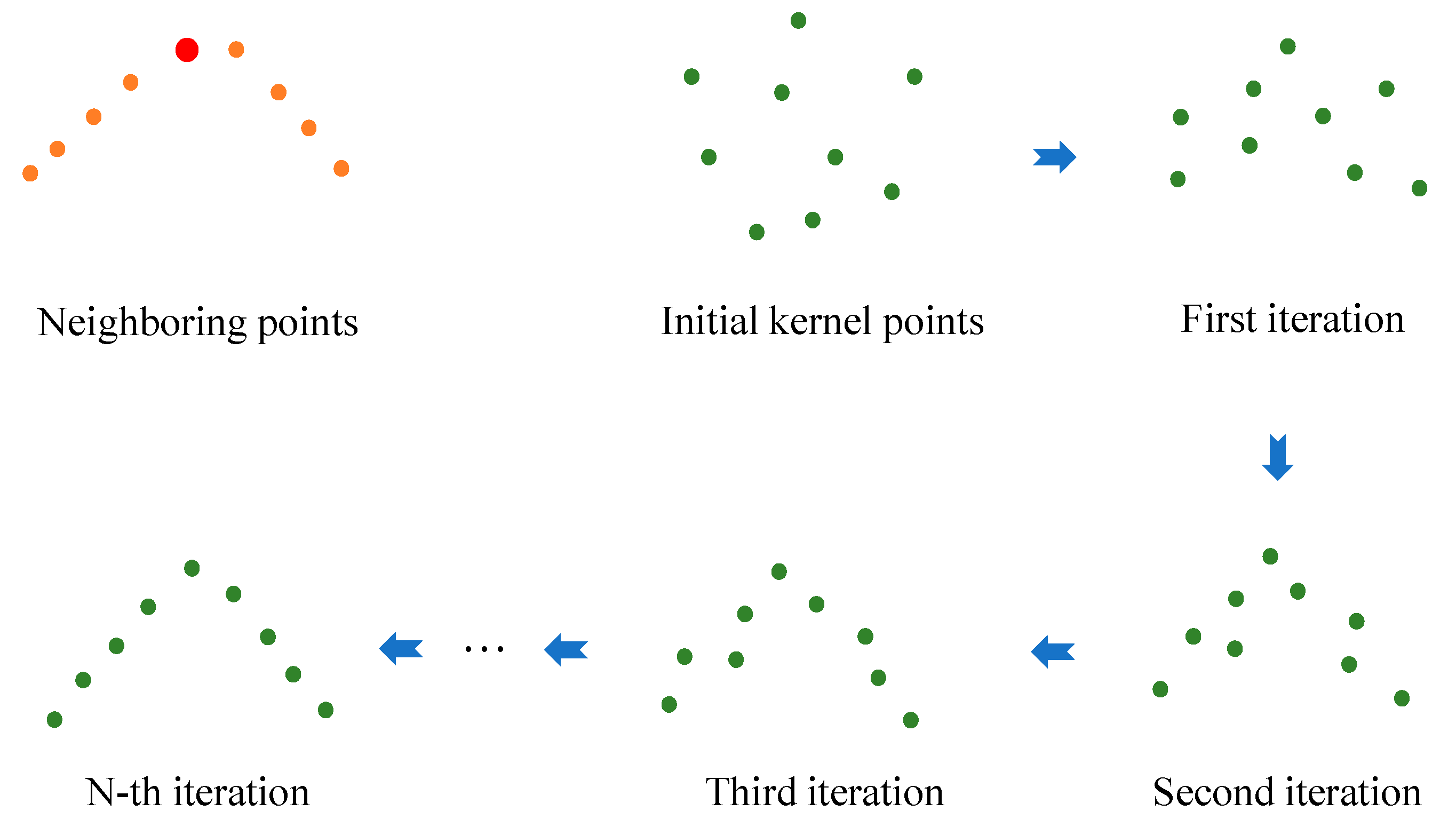
At the beginning of the training phase, the initial kernel points are uniformly scattered in a sphere, which means no meaningful geometric structures are formed by the convolution kernels and they cannot be used to match any geometric structures. During the training process, each convolution kernel is guided to approximate a specific geometric structure contained in the training data (an illustration of the training process of our SAC kernel is shown in Figure 2). Thus, our learned SAC kernels can be matched with and represent kinds of complex geometric structures that exist in real situations during the testing phase.

3.2. Relationship to Standard Convolution

3.2.1. Reformulation of Standard Convolution

We first revisit the standard convolution on regular 2D images (Figure 3). For each pixel of the regular image, we first need to find its neighboring pixels in a convolution window as a matrix I (here the image with a single channel is considered for convenience). We denote the convolution kernel as W, which is also a 2D matrix. Then, the convolution on the regular 2D image can be expressed as follows:
y = i , j W i , j   I i , j + b
where y represents the output of the convolution, i , j represents the index of the pixel in the neighbor patch or convolution kernel, and b is the corresponding bias.
More generally, if we flatten the matrix I and convolution kernel W to a one-dimensional vector with the same order, the above convolution on the regular image can reformulated as follows:
y = k W k I k + b = k C ( W k , I k ) + b
where C ( W k , I k ) is a function about the convolution kernel and the neighboring pixels. We can see that the convolution on the 2D image is actually a process of weighted summation of the neighboring pixels, where the values of the convolution kernel are the corresponding weights.

3.2.2. Reformulation of SAC

Similar to 2D images, our SAC also aims to aggregate the information in its neighboring region for each point, as shown in Equation (1). Suppose ϕ * is the optimization mapping function between the sets of neighboring points and kernel points in Equation (1). In practice, since || p ϕ * ( p ) || σ , the first-order Taylor expansion of the right side of Equation (1) is already a good approximation to s l . Therefore, we have the following:
s l = 1 | N i | p N i exp ( || p ϕ * ( p ) || 2 2 σ 2 ) A p N i || p ϕ * ( p ) || 2 + B = p N i K ( p , ϕ * ( p ) ) + B
where A and B are the parameters related to σ . Compared to the standard convolution in Equation (3), our SAC can actually be simplified as a similar formulation (Equation (4)) but with a modified convolution kernel function K ( p , ϕ * ( p ) ) .
However, unlike 2D images with regular data structure and their neighbors leveraging the natural fixed relative positions, the neighboring points of 3D point clouds can appear in any position of the 3D space and have no certain order. To handle this problem, a mapping function ϕ * : N i κ l that matches each neighboring point to its corresponding kernel point is needed, so that the kernel points can be applied to their corresponding neighboring points. Specifically, for each neighboring point p k N i , we should first find its corresponding kernel point ϕ * ( p k ) κ l , and the distance is then calculated between the corresponding point pair in the kernel and neighbor sets (as shown in Figure 3).

3.3. Deep Learning Networks with the Proposed SAC

According to the above analysis, our SAC actually provides a flexible geometric structure extractor which can be easily embedded into existing point cloud deep learning networks. In this section, we show how to construct the corresponding deep learning networks with our proposed SAC.
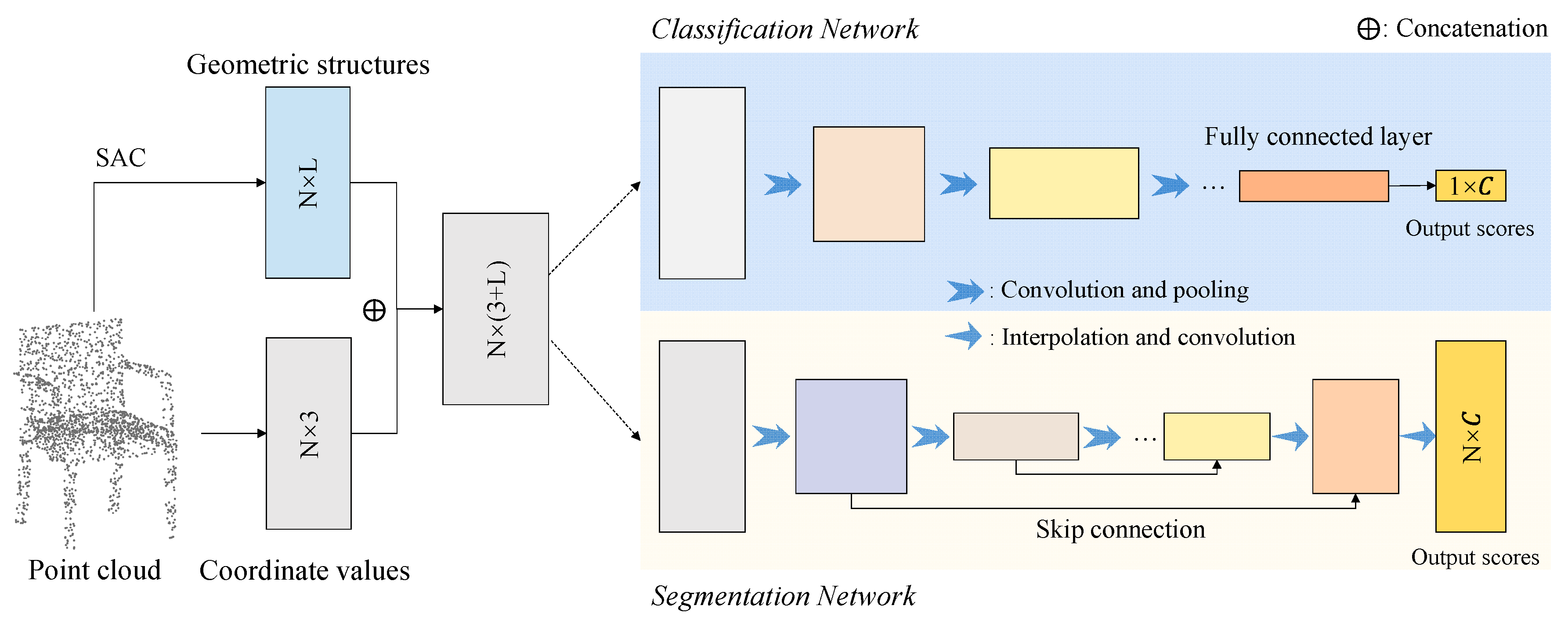
Specifically, the architecture of the classification and segmentation networks with our SAC is illustrated in Figure 4. For each point p i , we first find its neighboring points N i according to their spatial distance, and then match them with a series of 3D kernels κ l , l = 1 , 2 , , L . Therefore, the output of our SAC is an L -dimensional feature vector S = [ s 1 , s 2 , , s L ] , where each s l can be regarded as the matching degree between neighboring points and the l -th convolution kernel κ l . The geometric feature S is then used as the initial feature of each point for the subsequent classification or segmentation networks, which can be achieved with other state-of-the-art point cloud deep learning networks such as PointNet [1], PointNet++ [19], and KCNet [20].

4. Materials and Experiments

4.1. Tasks and Evaluation Metrics

To verify the effectiveness of our proposed SAC, we experimentally evaluated it on the following two tasks:
  • Object classification. The input of the classification task is the point cloud of the 3D object and our goal is to recognize which category it belongs to (e.g., airplane, car, or table);
  • Semantic segmentation. The input of the semantic segmentation task is the point cloud of the 3D scene, and it aims to assign each point a meaningful category label.
Note that our proposed SAC aims at capturing the geometric features directly from the coordinates of the neighboring points; it actually acts as a simple and efficient geometric feature extractor which can be embedded into other state-of-the-art point cloud deep learning networks. In this paper, three recently developed deep learning networks, PointNet [1], PointNet++ [19], and KCNet [20], were considered as the back-end networks, and our SAC was correspondingly embedded into them for performance evaluation. In addition, it is worth mentioning that all three deep learning networks can be applied for both classification and segmentation tasks. According to the difference of tasks, our SAC can be embedded into their corresponding versions for classification or semantic segmentation.
To quantitatively evaluate the performance of our SAC, two metrics including the overall accuracy (OA) and the intersection over union (IoU) were used in this work. Suppose there are C categories, p i j is the number of objects or points which belong to the i -th category but are predicted as the j -th category. Then, the OA can be formulated as follows:
O A = i = 1 C p i i i = 1 C j = 1 C p i j
the IoU for the i -th category is expressed as follows:
I o U i = p i i j = 1 C p i j + j = 1 C p j i p i i
and the corresponding mean IoU (mIoU) over all categories is m I o U = 1 C i = 1 C I o U i .

4.2. Object Classification Results

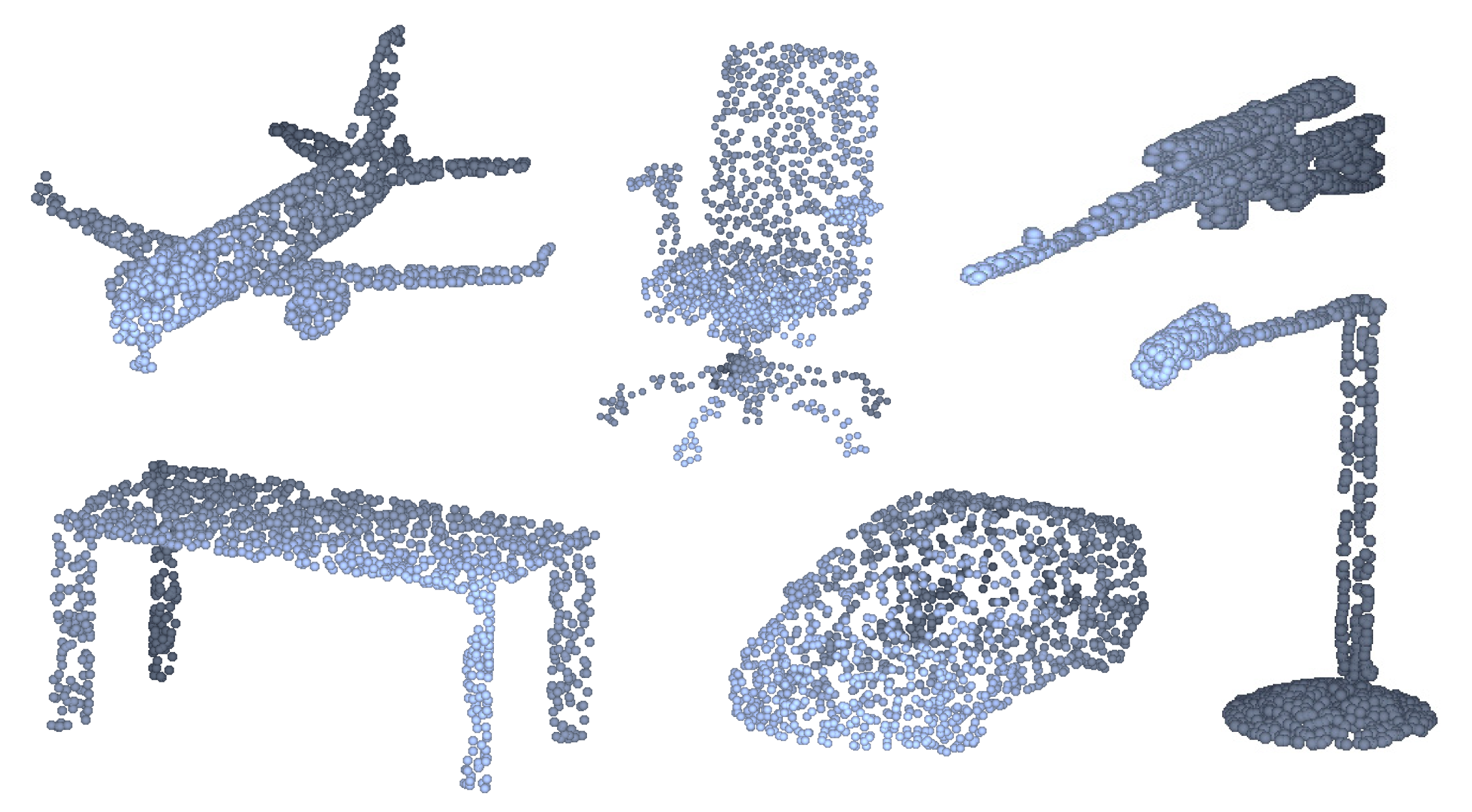
We first conducted our object classification experiments on the ModelNet40 dataset [13]. It consisted of 12,311 3D object models from 40 categories. Of these, 9843 were used as the training dataset, and the other 2468 objects were used as the testing dataset. In this experiment, we uniformly sampled 1024 points on each object model to convert it into a corresponding point cloud, as shown in Figure 5.
The input of the classification task is a point cloud of the corresponding 3D object, and the output is a category label for the object. To comprehensively evaluate the performance of our SAC, we constructed three classification networks by equipping the SAC with the classification networks of PointNet [1], PointNet++ [19], and KCNet [20], respectively, and named them SAPointNet, SAPointNet++, and SAKCNet for convenience.
The output dimension of our SAC was set as 32, and the number of kernel points was 17. For each point in the point cloud, we first found its 17 nearest neighbors (including itself) and matched them with 32 convolution kernels. Each kernel was also a point set containing 17 3D points, which corresponded to a specific geometric structure. When the geometric structure formed by the neighboring points was similar to the kernel, the corresponding point was activated. In addition, the remaining configurations were kept consistent with the original classification networks of PointNet, PointNet++, and KCNet for a fair comparison. All networks were trained with 250 epochs with a batch size of 32 on the training split of the ModelNet40 dataset [13], and their comparison results are provided in Table 1.
From Table 1, we can see that our classification networks integrated with SAC have consistently achieved higher accuracy compared to their original networks. Specifically, our SAPointNet achieved +4.92% accuracy over the original PointNet (vanilla) [1], whereas PointNet++ [19] and KCNet [20] were improved by +1.98% and +1.40%, respectively. Notably, by integrating local geometric structures of SAC with simple PointNet, our SAPointNet achieved better classification performance even than PointNet++ and KCNet, which shows the importance of accurate geometric structure representation for object classification.

4.3. Semantic Segmentation Results

4.3.1. Semantic Segmentation for Indoor Scene

In addition to object classification, we also applied our SAC to a semantic segmentation task to further evaluate its performance. In this section, we start from the semantic segmentation experiments on the Stanford Large-Scale 3D Indoor Spaces (S3DIS) dataset [53]. It is a large-scale indoor 3D point cloud dataset, which is collected in six large-scale indoor areas originating from three different buildings. Each point contains the x, y, and z coordinates and the corresponding RGB information, and is annotated as one of 13 object categories.
For a principled evaluation, Area 5 of the S3DIS dataset was chosen as the testing dataset and the remaining areas were used for network training in this experiment. Since Area 5 is not in the same buildings as the other areas and contains some different objects, this across-building experimental setup is more reasonable to measure the networks’ generalizability, while also bringing challenges to the semantic segmentation task.
To handle the enormous points in the 3D scenes, we first split the dataset room by room and then sliced them into 1 m by 1 m blocks. For each block, 4096 points were uniformly sampled for training convenience. During the testing phase, we first predicted the label for each sampled point, then the category label for the original points were assigned according to their nearest labeled point.
Similar to the object classification experiments, our SAC was further equipped with the segmentation version of PointNet [1], PointNet++ [19], and KCNet [20] to construct our corresponding segmentation networks. The output dimension of our SAC was also set as 32, and the number of kernel points was 17. However, instead of finding the 17 nearest neighbors for each point, we randomly sampled 17 points in a ball with 0.1 m radius, to reduce the influence of non-uniform point density. The remaining configurations were the same as PointNet, PointNet++, and KCNet. Following PointNet [1], all networks were trained with 50 epochs with a batch size of 24 on the training dataset.
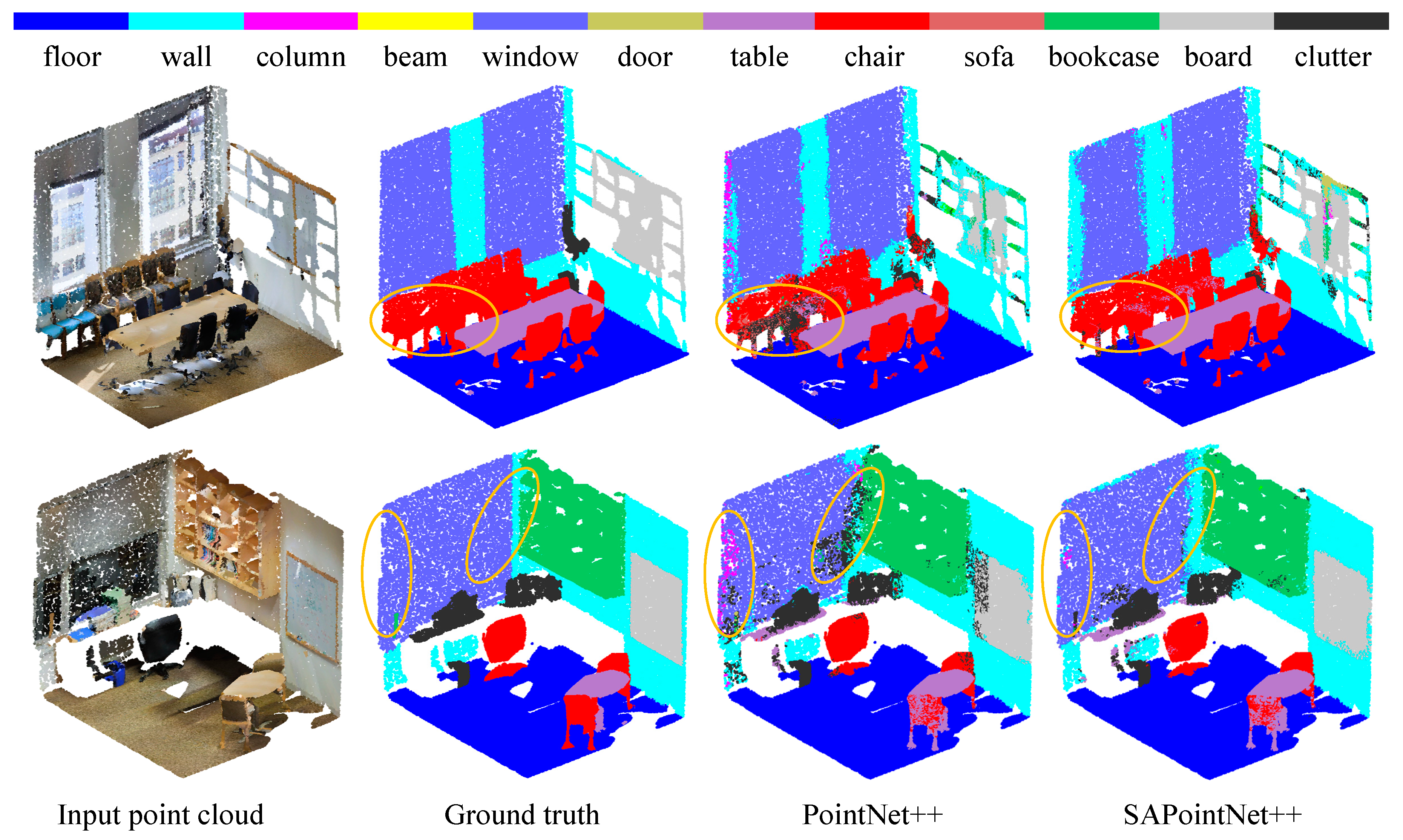
The quantitative and qualitative segmentation results on Area 5 of the S3DIS dataset are provided in Table 2 and Figure 6, respectively. We can see that our SAC shows consistent performance as compared to the above object classification task. Specifically, our proposed SAPointNet, SAPointNet++, and SAKCNet achieved +4.53%, +2.33%, and +2.07% mIoU over their corresponding back-end networks. In addition, we can also note that our SAC efficiently improved the segmentation accuracy on objects with rich geometric structures, such as chair, table, bookcase, and sofa. This further verifies the geometric feature representation capability of the proposed SAC.

4.3.2. Semantic Segmentation for Outdoor Scene

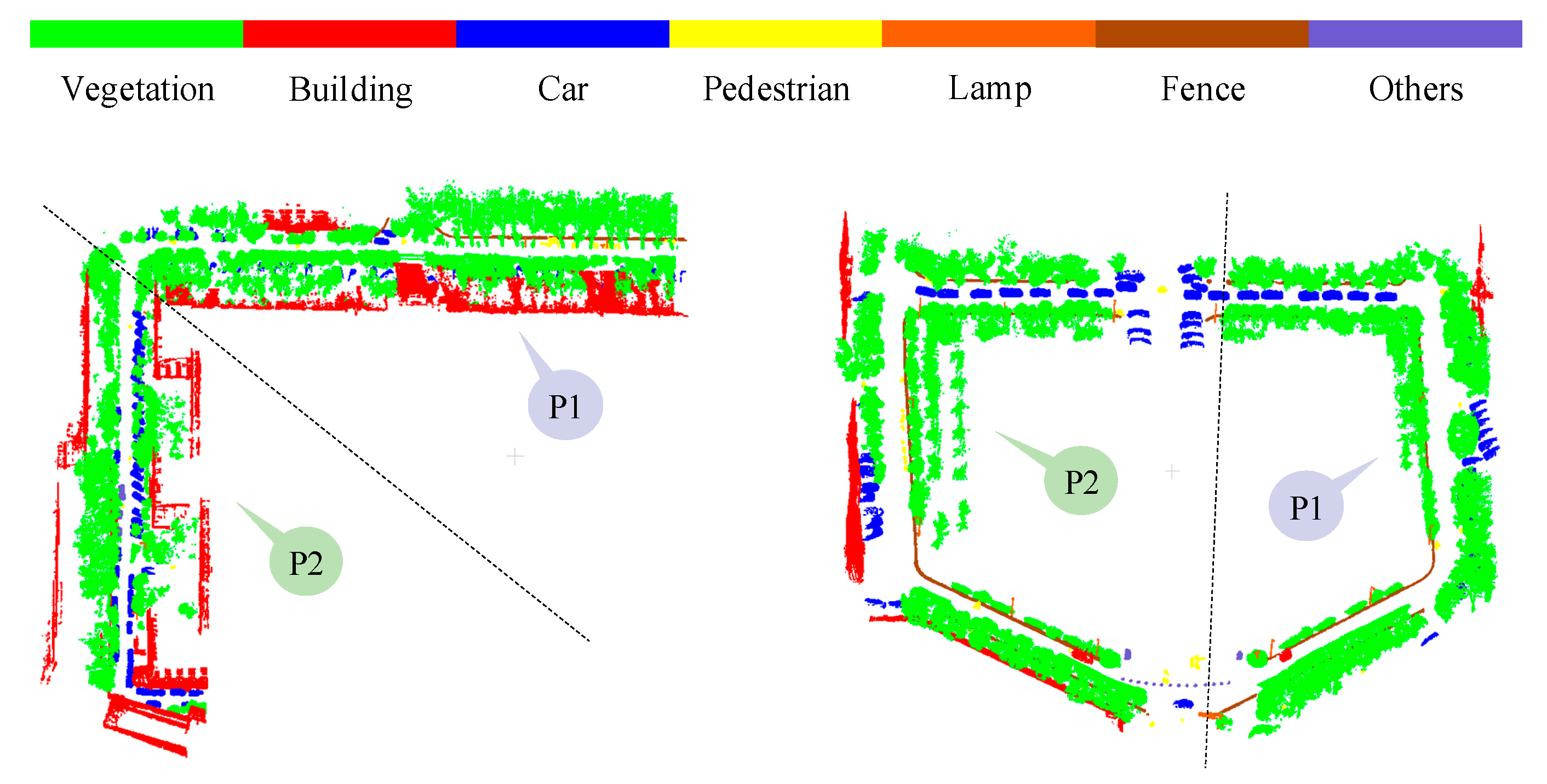
For this section, we further applied our SAC to the point cloud semantic segmentation task for an outdoor scene. To this end, the mobile laser scanning (MLS) point cloud from the campus of Wuhan University (WHU) [14] was used, as shown in Figure 7. This WHU MLS point cloud dataset contained two areas of the campus, and each area was split into training and testing datasets. Each point was labeled as one of seven categories: vegetation (e.g., tree and grass), building, car, pedestrian, lamp, fence, and others. In addition, compared to the S3DIS dataset, the point density of the WHU MLS point clouds varied greatly with the different distances between objects and scanners. Moreover, point clouds of many objects were incomplete due to mutual occlusion, which brings more challenges to the semantic segmentation task.
To adapt to the larger size of objects in the outdoor scene, we sliced the point clouds into 4 m by 4 m blocks while maintaining the same maximum number of 4096 points. In addition, the radius for neighborhood searching was set as 0.2 m. The other parts of the segmentation networks were kept consistent as the experiments for indoor scene segmentation. All networks were trained with 50 epochs with a batch size of 24 on the training dataset.
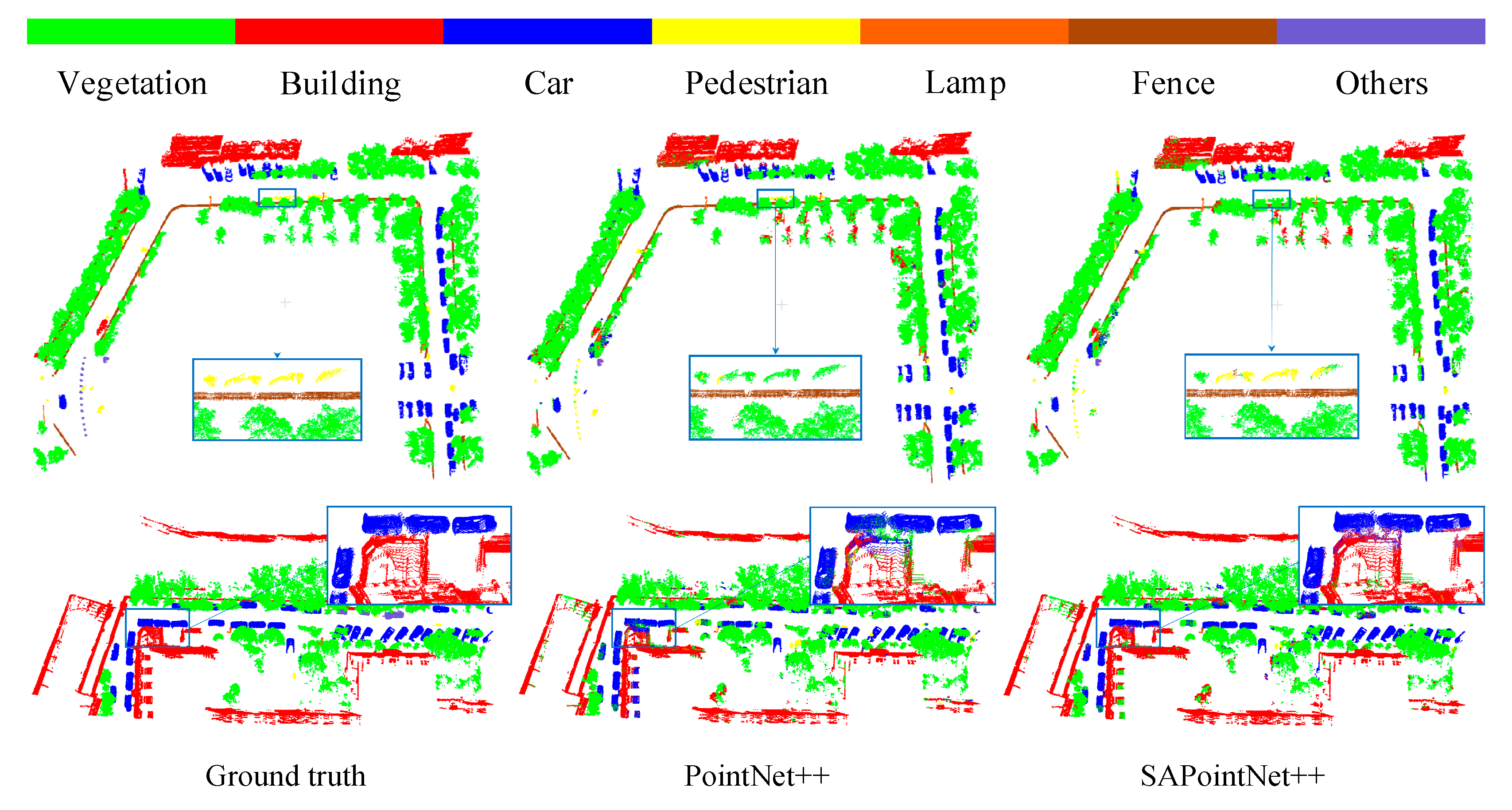
The quantitative testing results are provided in Table 3, and Figure 8 presents their segmentation results. We can see that our SAC achieved consistent performances as compared to the above experiments. The proposed SAPointNet, SAPointNet++, and SAKCNet achieved +15.01%, +3.66%, and +2.36% mIoU, respectively, over their corresponding back-end networks. Specifically, the accuracies on objects with rich geometric structures (e.g., car, pedestrian, lamp, fence) were efficiently improved with the proposed SAC, which further verifies its geometric feature learning capability.

5. Discussion

For this section, we conducted more experiments to further explore and discuss the performances and properties of the proposed SAC.

5.1. Parametric Sensitivity Analysis

We started by analyzing the sensitivity of the parameters in our proposed SAC. According to the above description, the three parameters were the number of convolution kernels, the number of points contained in each convolution kernel, and the constant parameter σ (Section 3.1). The number of convolution kernels corresponded to the output channel of our SAC, whereas the number of kernel points determined the size of the convolution kernel. According to the commonly used convolution parameters for 2D images, we similarly considered several choices for these parameters to analyze their influences.
In Table 4, we provide detailed classification accuracy of the ModelNet40 dataset [13] using the proposed SAPointNet. We can see that with an increased number of convolution kernels, more geometric structures can be represented by our SAC for accurate object classification, and the number of kernel points shows a consistent pattern. However, considering the balance between performance and efficiency, the number of convolution kernels and kernel points were set to 32 and 17, respectively, in this paper. In addition, according to the shape of the Gaussian function, smaller or larger σ makes the outputs tend toward 0 or 1 and the difference between the output values tends toward 0, which is harmful for geometric feature representation. Thus, the parameter σ = 0.05 was finally used in our experiments.

5.2. KNN vs. Ball Query

The two alternative local neighborhood searching methods are k-nearest neighbors (KNN) and radius-based ball query. For our object classification task on the ModelNet40 dataset [13], the 17 nearest points were selected as the neighbor set for each point, whereas the 17 neighboring points within a local ball were selected for semantic segmentation experiments for both indoor and outdoor 3D scenes. For this section, we conducted more experiments to discuss the performance differences between KNN and ball query.
In Table 5 and Table 6, we provide the classification and segmentation results, respectively, using KNN and ball query. Interestingly, we note that KNN is better than ball query for the object classification task, but it is the opposite for the semantic segmentation task. Because of the non-uniform point density of the indoor and outdoor 3D scenes, neighborhood searching in a local ball can reduce the influence of varied point density and noise. However, for point clouds that are uniformly sampled from ModelNet40 3D objects, the searching window of KNN can be adaptively changed and shows better performance.

5.3. Latent Visualization

Good features should be discriminative, which means that features of the same object category should be close to each other, whereas the features from different object categories should be far away from each other. The deep learning network can be regarded as two phases, namely feature extraction and classification. The network first maps the input point clouds into a latent feature space, where the point clouds can be easily distinguished and classified.
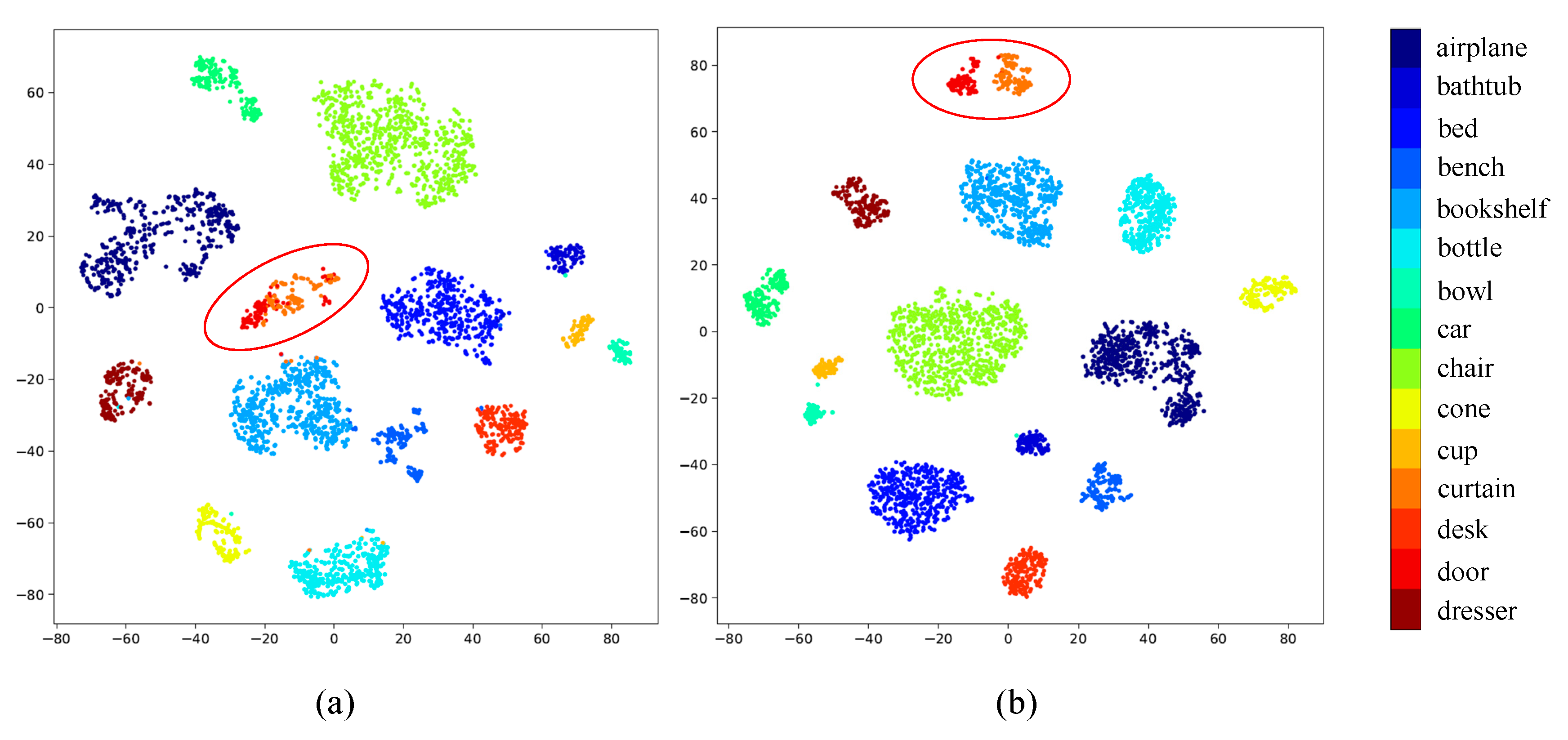
To further verify the effectiveness of the proposed SAC, we provided more visualization of the extracted features on the ModelNet40 dataset [13]. Specifically, the features in the last fully connected layer of PointNet and our SAPointNet were visualized in this experiment. However, since the extracted features always had high dimensions (e.g., the feature dimension of our classification network was set as 256), t-SNE [54] was applied here to project the features onto a 2D plane. In addition, for visual convenience, only the first 15 object categories of the ModelNet40 dataset were selected, and their feature visualizations are provided in Figure 9. Compared to PointNet, the features learned by our SAPointNet show better distinguishability for different categories, which is important for the further classification tasks.

5.4. Visualization of the Learned Kernels

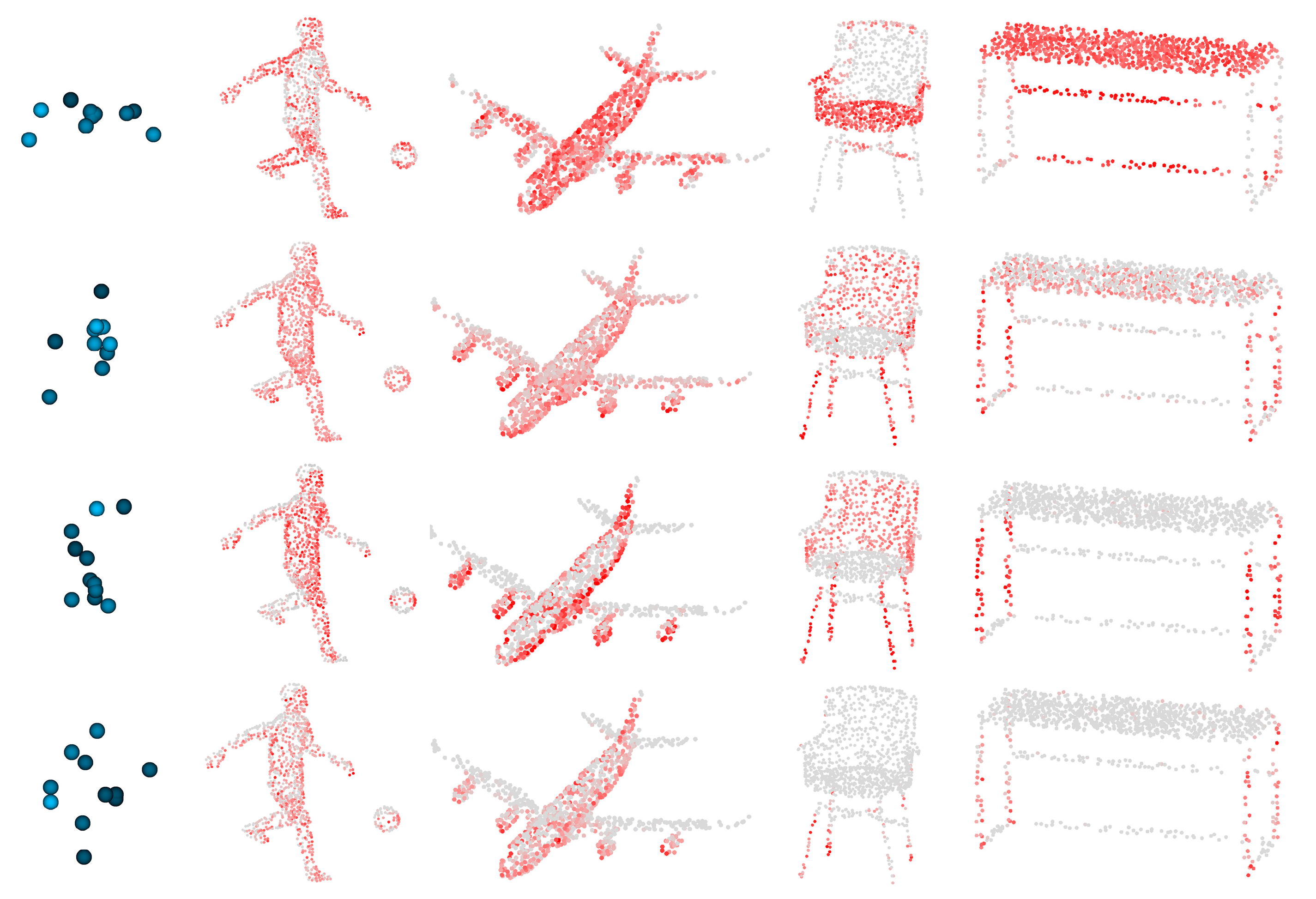
In this section, we provide more visualizations of the learned kernels. Our SAC was designed to capture geometric features with a series of learnable kernels. The geometric structures formed by the kernels can be adaptively adjusted to match the similar structures in the point clouds. To give an intuitive visualization, the learned kernels (consisting of a set of 3D points) are rendered in Figure 10, as well as their corresponding activations on the input point clouds.
However, why are the structures formed by the learned kernels not the regular common geometric structures (e.g., line, plane, or corner)? Actually, since the directions of geometric structures in real situations are arbitrary and complex, simple geometric structures (e.g., line, plane) with specific directions are difficult to adapt to structures with arbitrary directions. Therefore, the geometric structures of our learned kernels are correspondingly distorted in the 3D space, in order to be matched with as many geometric structures in real situations as possible.

5.5. Robustness Test

To fully understand the performance of our SAC under the disturbance of noise, we further conducted several robustness tests for this section. Note that the additional noise changes the class attributes of the points in the segmentation task and that our robustness tests are only conducted on the classification task with the ModelNet40 dataset [13].
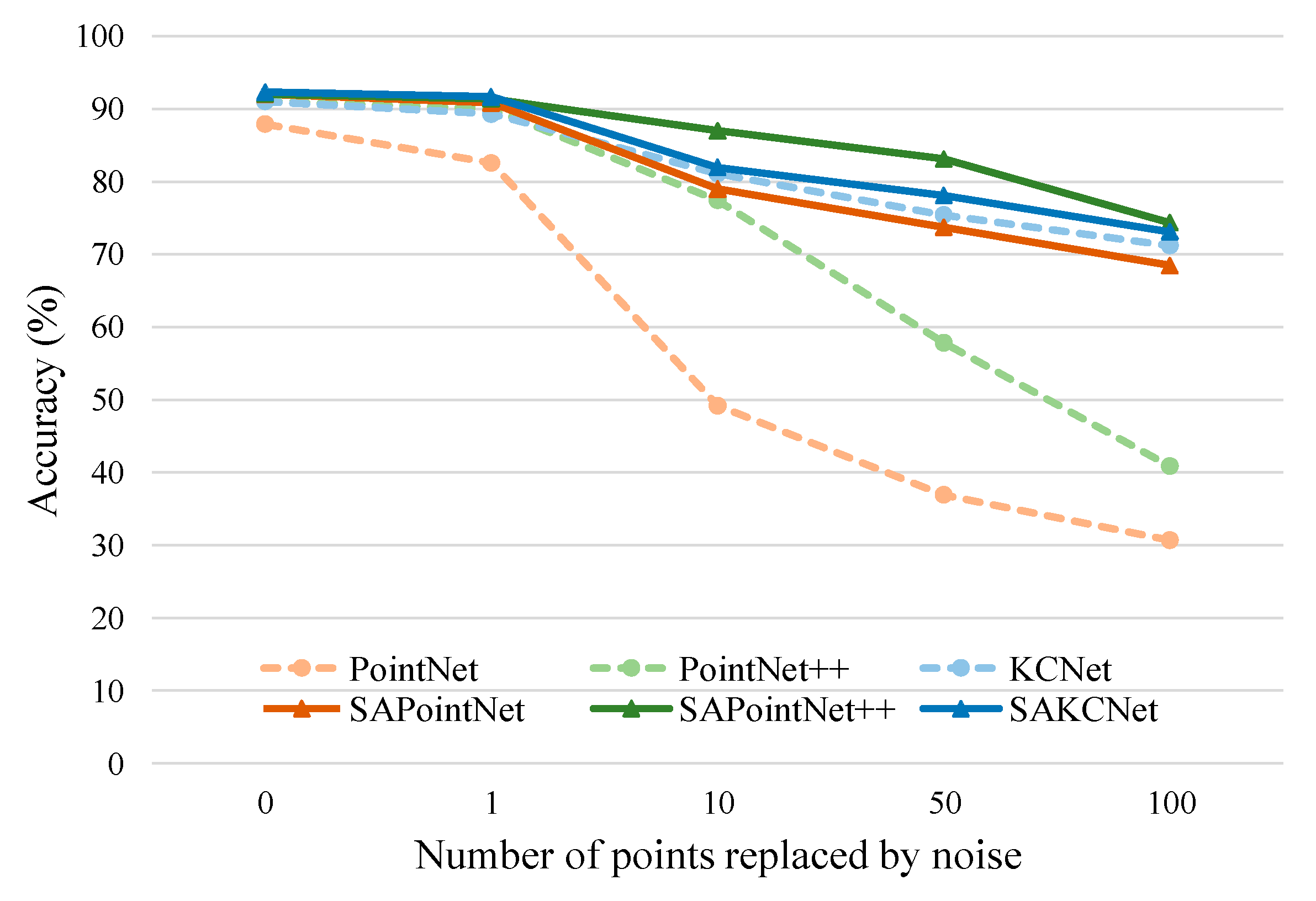
Specifically, for each object in the testing dataset, some of the points are randomly replaced by the uniform noises lying in [ 1 , 1 ] 3 . All the networks are trained on the ModelNet40 training dataset without the disturbance of noise. In addition, to avoid random deviations during the experiments, all results were tested five times, and their averages are reported. Results of robustness tests are presented in Figure 11. We can see that PointNet is most sensitive to noises, followed by PointNet++. At the same time, benefiting from the structure representation capability of our SAC, the robustness of these back-end networks is efficiently improved.

6. Conclusions and Future Works

We propose a novel structure-aware convolution (SAC) to learn the geometric structures of 3D point clouds. The key of our SAC is to match the input 3D point clouds with a series of learnable 3D kernels, which can be seen as the “templates” with specific geometric structures learned from the training dataset.
Our SAC is a lightweight yet efficient module that can be easily integrated with existing state-of-the-art point cloud deep learning networks. To verify the performance of the proposed SAC, we integrated it with three recently developed networks, PointNet [1], PointNet++ [19], and KCNet [20], for both object classification and semantic segmentation tasks of 3D point clouds. Experimental results show that, benefiting from the geometric structure learning capability of our SAC, the performance of PointNet, PointNet++, and KCNet can be efficiently improved with few additional parameters (e.g., +2.77% mean classification accuracy and +4.99% mean segmentation IoU). Moreover, with the integration of SAC, these back-end networks have also shown better robustness to noise.
In the future, two main aspects can be considered to improve or extend our proposed SAC. (1) Adding rotation freedom for the kernels. Since the kernels in our SAC are directly matched with the input point clouds, geometric structures with arbitrary directions are difficult to represent with finite kernels. Thus, preadjusting the direction of the kernels to align them with the real point clouds would be helpful to improve the performance of SAC. (2) Extending SAC to the feature space. The proposed SAC aims at capturing the local geometric structures directly from 3D point clouds. However, the “structure” also exists in high-dimensional feature space, and our SAC can also be extended to explore such relations between features.

Author Contributions

L.W. designed the framework of this research and performed the experiments; L.W., Y.L., and S.Z. wrote the paper; P.T. and J.Y. offered advice on this research and edited the paper. All authors read and agreed to the published version of the manuscript.

Funding

This work was supported by the National Natural Science Foundation of China (Nos. 41801390 and 41801387) and the National Key R&D Program of China (No. 2017YFB0503004).

Acknowledgments

We are thankful to anonymous reviewers for their helpful comments and suggestions, and other researchers for their open-source projects.

Conflicts of Interest

The authors declare no conflict of interest.

References

  1. Qi, C.R.; Su, H.; Mo, K.; Guibas, L.J. PointNet: Deep Learning on Point Sets for 3D Classification and Segmentation. In Proceedings of the IEEE Conference on Computer Vision and Pattern Recognition, Honolulu, HI, USA, 21–26 July 2017; pp. 77–85. [Google Scholar]
  2. Liu, Y.; Fan, B.; Xiang, S.; Pan, C. Relation-Shape Convolutional Neural Network for Point Cloud Analysis. In Proceedings of the IEEE Conference on Computer Vision and Pattern Recognition, Long Beach, CA, USA, 16–20 June 2019; pp. 8895–8904. [Google Scholar]
  3. Zheng, M.; Wu, H.; Li, Y. An adaptive end-to-end classification approach for mobile laser scanning point clouds based on knowledge in urban scenes. Remote Sens. 2019, 11, 186. [Google Scholar] [CrossRef] [Green Version]
  4. Krizhevsky, A.; Sutskever, I.; Hinton, G.E. ImageNet Classification with Deep Convolutional Neural Networks. Available online: http://papers.nips.cc/paper/4824-imagenet-classification-with-deep-convolutional-neural-networ (accessed on 14 February 2020).
  5. He, K.; Zhang, X.; Ren, S.; Sun, J. Deep Residual Learning for Image Recognition. In Proceedings of the IEEE Conference on Computer Vision and Pattern Recognition, Las Vegas, NV, USA, 26 June–1 July 2016; pp. 770–778. [Google Scholar]
  6. Chen, L.C.; Papandreou, G.; Kokkinos, I.; Murphy, K.; Yuille, A.L. DeepLab: Semantic Image Segmentation with Deep Convolutional Nets, Atrous Convolution, and Fully Connected CRFs. IEEE Trans. Pattern Anal. Mach. Intell. 2018, 40, 834–848. [Google Scholar] [CrossRef] [PubMed]
  7. Wang, L.; Huang, Y.; Hou, Y.; Zhang, S.; Shan, J. Graph Attention Convolution for Point Cloud Semantic Segmentation. In Proceedings of the IEEE Conference on Computer Vision and Pattern Recognition, Long Beach, CA, USA, 16–20 June 2019; pp. 10296–10305. [Google Scholar]
  8. Graham, B.; Engelcke, M.; van der Maaten, L. 3D Semantic Segmentation with Submanifold Sparse Convolutional Networks. In Proceedings of the IEEE Conference on Computer Vision and Pattern Recognition, Salt Lake City, UT, USA, 18–23 June 2018; pp. 9224–9232. [Google Scholar]
  9. Tchapmi, L.P.; Choy, C.B.; Armeni, I.; Gwak, J.; Savarese, S. SEGCloud: Semantic Segmentation of 3D Point Clouds. In Proceedings of the 2017 International Conference on 3D Vision, Qingdao, China, 10–12 October 2017; pp. 537–547. [Google Scholar]
  10. Yang, Z.; Jiang, W.; Xu, B.; Zhu, Q.; Jiang, S.; Huang, W. A convolutional neural network-based 3D semantic labeling method for ALS point clouds. Remote Sens. 2017, 9, 936. [Google Scholar] [CrossRef] [Green Version]
  11. Gadelha, M.; Wang, R.; Maji, S. Multiresolution Tree Networks for 3D Point Cloud Processing. In Proceedings of the European Conference on Computer Vision, Munich, Germany, 8–14 September 2018; pp. 103–118. [Google Scholar]
  12. Maturana, D.; Scherer, S. VoxNet: A 3D Convolutional Neural Network for Real-Time Object Recognition. In Proceedings of the IEEE International Conference on Intelligent Robots and Systems, Hamburg, Germany, 28 September–2 October 2015; pp. 922–928. [Google Scholar]
  13. Wu, Z.; Song, S.; Khosla, A.; Yu, F.; Zhang, L.; Tang, X.; Xiao, J. 3D ShapeNets: A Deep Representation for Volumetric Shapes. In Proceedings of the IEEE Conference on Computer Vision and Pattern Recognition, Boston, MA, USA, 7–12 June 2015; pp. 1912–1920. [Google Scholar]
  14. Wang, L.; Huang, Y.; Shan, J.; He, L. MSNet: Multi-scale convolutional network for point cloud classification. Remote Sens. 2018, 10, 612. [Google Scholar] [CrossRef] [Green Version]
  15. Feng, Y.; Zhang, Z.; Zhao, X.; Ji, R.; Gao, Y. GVCNN: Group-View Convolutional Neural Networks for 3D Shape Recognition. In Proceedings of the IEEE Conference on Computer Vision and Pattern Recognition, Salt Lake City, UT, USA, 18–23 June 2018; pp. 264–272. [Google Scholar]
  16. Su, H.; Maji, S.; Kalogerakis, E.; Learned-Miller, E. Multi-view Convolutional Neural Networks for 3D Shape Recognition. In Proceedings of the IEEE International Conference on Computer Vision, Santiago, Chile, 11–18 December 2015; pp. 945–953. [Google Scholar]
  17. Kalogerakis, E.; Averkiou, M.; Maji, S.; Chaudhuri, S. 3D Shape Segmentation with Projective Convolutional Networks. In Proceedings of the IEEE Conference on Computer Vision and Pattern Recognition, Honolulu, HI, USA, 21–26 July 2017; pp. 6630–6639. [Google Scholar]
  18. Le, T.; Bui, G.; Duan, Y. A multi-view recurrent neural network for 3D mesh segmentation. Comput. Graph. 2017, 66, 103–112. [Google Scholar] [CrossRef]
  19. Qi, C.R.; Yi, L.; Su, H.; Guibas, L.J. PointNet++: Deep Hierarchical Feature Learning on Point Sets in a Metric Space. Available online: http://papers.nips.cc/paper/7095-pointnet-deep-hierarchical-feature-learning-on-point-se (accessed on 14 February 2020).
  20. Shen, Y.; Feng, C.; Yang, Y.; Tian, D. Mining Point Cloud Local Structures by Kernel Correlation and Graph Pooling. In Proceedings of the IEEE Conference on Computer Vision and Pattern Recognition, Salt Lake City, UT, USA, 18–23 June 2018; pp. 4548–4557. [Google Scholar]
  21. Rusu, R.B.; Blodow, N.; Beetz, M. Fast Point Feature Histograms (FPFH) for 3D registration. In Proceedings of the IEEE International Conference on Robotics and Automation, Kobe, Japan, 12–17 May 2009; pp. 3212–3217. [Google Scholar]
  22. Salti, S.; Tombari, F.; Di Stefano, L. SHOT: Unique signatures of histograms for surface and texture description. Comput. Vis. Image Underst. 2014, 125, 251–264. [Google Scholar] [CrossRef]
  23. Xu, Y.; Ye, Z.; Yao, W.; Huang, R.; Tong, X.; Hoegner, L.; Stilla, U. Classification of LiDAR Point Clouds Using Supervoxel-Based Detrended Feature and Perception-Weighted Graphical Model. IEEE J. Sel. Top. Appl. Earth Obs. Remote Sens. 2019, 13, 72–88. [Google Scholar] [CrossRef]
  24. Niemeyer, J.; Rottensteiner, F.; Soergel, U. Contextual classification of lidar data and building object detection in urban areas. ISPRS J. Photogramm. Remote Sens. 2014, 87, 152–165. [Google Scholar] [CrossRef]
  25. Weinmann, M.; Schmidt, A.; Mallet, C.; Hinz, S.; Rottensteiner, F.; Jutzi, B. Contextual classification of point cloud data by exploiting individual 3D neigbourhoods. ISPRS Ann. Photogramm. Remote Sens. Spat. Inf. Sci. 2015, 2, 271–278. [Google Scholar] [CrossRef] [Green Version]
  26. Richter, R.; Behrens, M.; Döllner, J. Object class segmentation of massive 3D point clouds of urban areas using point cloud topology. Int. J. Remote Sens. 2013, 34, 8408–8424. [Google Scholar] [CrossRef]
  27. Anand, A.; Koppula, H.S.; Joachims, T.; Saxena, A. Contextually guided semantic labeling and search for three-dimensional point clouds. Int. J. Robot. Res. 2013, 32, 19–34. [Google Scholar] [CrossRef]
  28. Chen, G.; Maggioni, M. Multiscale Geometric Dictionaries for Point-Cloud Data. In Proceedings of the International Conference on Sampling Theory and Applications (SampTA), Singapore, 2–6 May 2011; Volume 4. [Google Scholar]
  29. Zhang, Z.; Zhang, L.; Tong, X.; Mathiopoulos, P.T.; Guo, B.; Huang, X.; Wang, Z.; Wang, Y. A Multilevel Point-Cluster-Based Discriminative Feature for ALS Point Cloud Classification. IEEE Trans. Geosci. Remote Sens. 2016, 54, 3309–3321. [Google Scholar] [CrossRef]
  30. Hackel, T.; Wegner, J.D.; Schindler, K. Fast semantic segmentation of 3D point clouds with strongly varying density. ISPRS Ann. Photogramm. Remote Sens. Spat. Inf. Sci. 2016, 3, 177–184. [Google Scholar] [CrossRef]
  31. Zhang, J.; Lin, X.; Ning, X. SVM-Based classification of segmented airborne LiDAR point clouds in urban areas. Remote Sens. 2013, 5, 3749–3775. [Google Scholar] [CrossRef] [Green Version]
  32. Ghamisi, P.; Höfle, B. LiDAR Data Classification Using Extinction Profiles and a Composite Kernel Support Vector Machine. IEEE Geosci. Remote Sens. Lett. 2017, 14, 659–663. [Google Scholar] [CrossRef]
  33. Lodha, S.K.; Fitzpatrick, D.M.; Helmbold, D.P. Aerial Lidar Data Classification Using AdaBoost. In Proceedings of the 6th International Conference on 3-D Digital Imaging and Modeling, Montreal, QC, Canada, 21–23 August 2007; pp. 435–442. [Google Scholar]
  34. Niemeyer, J.; Rottensteiner, F.; Soergel, U. Classification of Urban LiDAR Data Using Conditional Random Field and Random Forests. In Proceedings of the Joint Urban Remote Sensing Event, Sao Paulo, Brazil, 21–23 April 2013; Volume 856, pp. 139–142. [Google Scholar]
  35. Ni, H.; Lin, X.; Zhang, J. Classification of ALS point cloud with improved point cloud segmentation and random forests. Remote Sens. 2017, 9, 288. [Google Scholar] [CrossRef] [Green Version]
  36. Najafi, M.; Namin, S.T.; Salzmann, M.; Petersson, L. Non-Associative Higher-Order Markov Networks for Point Cloud Classification. In Proceedings of the European Conference on Computer Vision, Zurich, Switzerland, 6–12 September 2014; pp. 500–515. [Google Scholar]
  37. Niemeyer, J.; Rottensteiner, F.; Soergel, U. Conditional random fields for LiDAR point cloud classification in complex urban areas. ISPRS Ann. Photogramm. Remote Sens. Spatioal Inf. Sci. 2012, 3, 263–268. [Google Scholar] [CrossRef] [Green Version]
  38. Niemeyer, J.; Rottensteiner, F.; Soergel, U.; Heipke, C. Hierarchical higher order crf for the classification of airborne lidar point clouds in urban areas. Int. Arch. Photogramm. Remote Sens. Spat. Inf. Sci. 2016, 41, 655–662. [Google Scholar] [CrossRef] [Green Version]
  39. Yan, J.; Shan, J.; Jiang, W. A global optimization approach to roof segmentation from airborne lidar point clouds. ISPRS J. Photogramm. Remote Sens. 2014, 94, 183–193. [Google Scholar] [CrossRef]
  40. Le, T.; Duan, Y. PointGrid: A Deep Network for 3D Shape Understanding. In Proceedings of the IEEE Conference on Computer Vision and Pattern Recognition, Salt Lake City, UT, USA, 18–23 June 2018; pp. 9204–9214. [Google Scholar]
  41. Wang, P.-S.; Liu, Y.; Guo, Y.-X.; Sun, C.-Y.; Tong, X. O-CNN: Octree-based Convolutional Neural Networks for 3D Shape Analysis. ACM Trans. Graph. 2017, 36, 1–11. [Google Scholar] [CrossRef]
  42. Bronstein, M.M.; Bruna, J.; Lecun, Y.; Szlam, A.; Vandergheynst, P. Geometric Deep Learning: Going beyond Euclidean data. IEEE Signal Process. Mag. 2017, 34, 18–42. [Google Scholar] [CrossRef] [Green Version]
  43. Simonovsky, M.; Komodakis, N. Dynamic Edge-Conditioned Filters in Convolutional Neural Networks on Graphs. In Proceedings of the IEEE Conference on Computer Vision and Pattern Recognition, Honolulu, HI, USA, 21–26 July 2017; pp. 29–38. [Google Scholar]
  44. Yi, L.; Su, H.; Guo, X.; Guibas, L.J. SyncSpecCNN: Synchronized Spectral CNN for 3D Shape Segmentation. In Proceedings of the IEEE Conference on Computer Vision and Pattern Recognition, Honolulu, HI, USA, 21–26 July 2017; pp. 6584–6592. [Google Scholar]
  45. Landrieu, L.; Simonovsky, M. Large-scale Point Cloud Semantic Segmentation with Superpoint Graphs. In Proceedings of the IEEE Conference on Computer Vision and Pattern Recognition, Salt Lake City, UT, USA, 18–23 June 2018. [Google Scholar]
  46. Engelmann, F.; Kontogianni, T.; Hermans, A.; Leibe, B. Exploring Spatial Context for 3D Semantic Segmentation of Point Clouds. In Proceedings of the IEEE International Conference on Computer Vision Workshop, Venice, Italy, 22–29 October 2017; pp. 716–724. [Google Scholar]
  47. Ravanbakhsh, S.; Schneider, J.; Poczos, B. Deep Learning with Sets and Point Clouds. arXiv Prepr. 2016, arXiv:1611.04500. [Google Scholar]
  48. Zaheer, M.; Kottur, S.; Ravanbakhsh, S.; Poczos, B.; Salakhutdinov, R.; Smola, A. Deep Sets. Available online: http://papers.nips.cc/paper/6931-deep-sets (accessed on 14 February 2020).
  49. Xu, Y.; Fan, T.; Xu, M.; Zeng, L.; Qiao, Y. Spidercnn: Deep Learning on Point Sets with Parameterized Convolutional Filters. In Proceedings of the European Conference on Computer Vision, Munich, Germany, 8–14 September 2018; pp. 87–102. [Google Scholar]
  50. Komarichev, A.; Zhong, Z.; Hua, J. A-CNN: Annularly Convolutional Neural Networks on Point Clouds. In Proceedings of the IEEE Conference on Computer Vision and Pattern Recognition, Long Beach, CA, USA, 16–20 June 2019; pp. 7421–7430. [Google Scholar]
  51. Thomas, H.; Qi, C.R.; Deschaud, J.-E.; Marcotegui, B.; Goulette, F.; Guibas, L.J. KPConv: Flexible and Deformable Convolution for Point Clouds. In Proceedings of the IEEE International Conference on Computer Vision, Seoul, Korea, 27 October–2 November 2019; pp. 6411–6420. [Google Scholar]
  52. Atzmon, M.; Maron, H.; Lipman, Y. Point convolutional neural networks by extension operators. ACM Trans. Graph. 2018, 37, 1–12. [Google Scholar] [CrossRef] [Green Version]
  53. Armeni, I.; Sener, O.; Zamir, A.R.; Jiang, H.; Brilakis, I.; Fischer, M.; Savarese, S. 3D Semantic Parsing of Large-Scale Indoor Spaces. In Proceedings of the IEEE Conference on Computer Vision and Pattern Recognition, Las Vegas, NV, USA, 26 June–1 July 2016; pp. 1534–1543. [Google Scholar]
  54. Maaten, L.V.D.; Hinton, G. Visualizing data using t-SNE. J. Mach. Learn. Res. 2008, 9, 2579–2605. [Google Scholar]
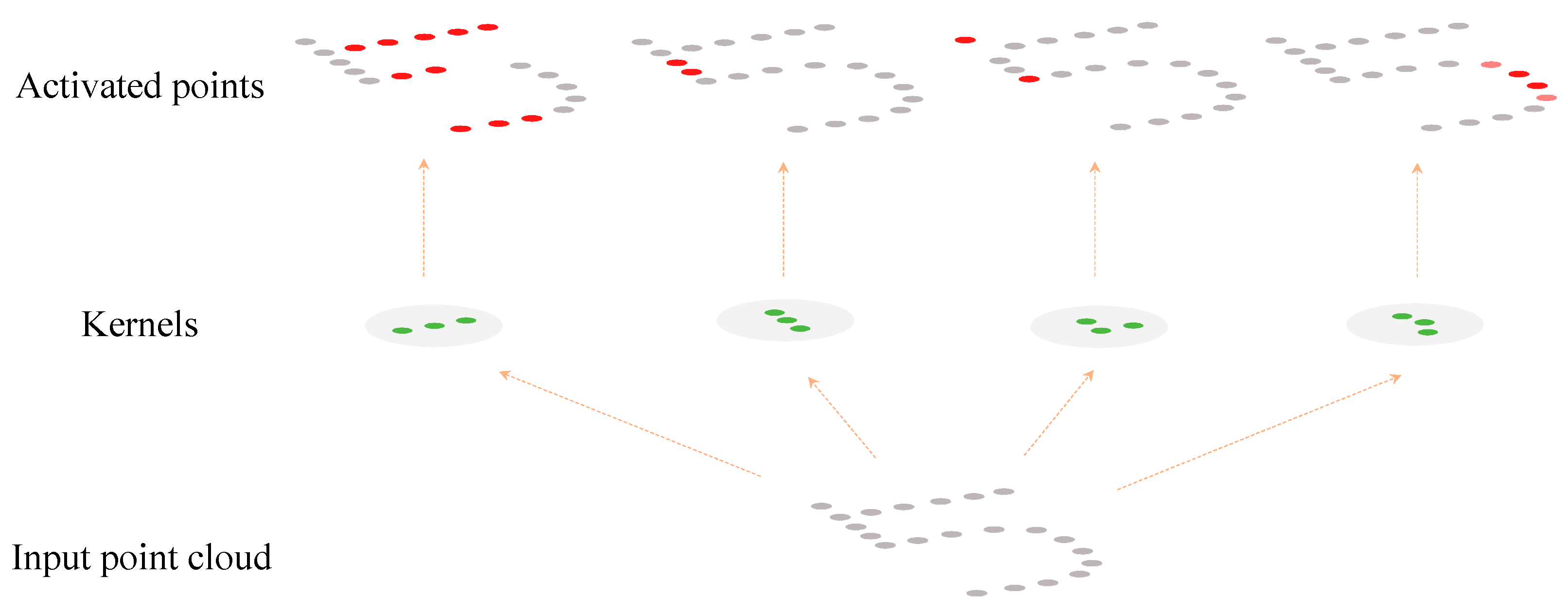
Figure 1. Illustration of kernels and their matching results on the input point cloud. For each point of the input point cloud, we first find its three neighbors and then match them with different kernels. When the local geometric structure is similar to the kernel, the current point is activated correspondingly (darker red means larger activated value).
Remotesensing 12 00634 g001
Figure 2. Illustration of the training process of our structure-aware convolution (SAC). The kernel points’ coordinates are randomly initialized using a uniform distribution. With training iteration, the kernel points’ coordinates are gradually adjusted so that they can be well matched with one kind of geometric structure formed by the neighboring points in real situations. The learned kernels can then be used to capture the interested structures in 3D point clouds during the test phase.
Remotesensing 12 00634 g002
Figure 3. Illustration of 2D convolution and SAC. (a) Illustration of the convolution on the 2D image, which can be represented as a weighted combination of the neighboring pixels’ features (The standard convolution should first transpose the convolution kernels and then multiply them with the corresponding pixels. We omit the transposition process here for denotation convenience.); (b) Illustration of the proposed SAC on the 3D point cloud. Kernel points are matched with neighbors of each point; the point with a local geometric structure similar to the kernel is activated. Both the 2D convolution and our SAC aim at detecting specific patterns in images or point clouds. However, the patterns are reflected by changing gray values in images, but are shown by spatial coordinates in point clouds.
Remotesensing 12 00634 g003
Figure 4. Architecture of the proposed point cloud deep learning networks. The output of our SAC is an L-dimensional geometric feature vector for each point, which can be easily combined with other point cloud deep learning networks. In this work, both classification and segmentation networks are constructed with our SAC. The output of the classification network is a category label for the entire point cloud, while the segmentation network aims to assign each point a reasonable category label. The classification and segmentation networks can be implemented using other existing point cloud deep learning networks (e.g., PointNet, PointNet++, and KCNet), and their detailed architectures and parameters are then subsequently determined.
Remotesensing 12 00634 g004
Figure 5. Point clouds sampled from 3D objects in the ModelNet40 dataset. All point clouds are normalized into a unit sphere for convenience.
Remotesensing 12 00634 g005
Figure 6. Semantic segmentation results on the S3DIS dataset. Two conference rooms and their segmentation results with PointNet++ [19] and our SAPointNet++ are provided since their multi-scale feature learning mechanism is more suitable for the semantic segmentation task. For visual convenience, the ceiling of each room and parts of wall are not shown.
Remotesensing 12 00634 g006
Figure 7. Illustration of the mobile laser scanning (MLS) point clouds from Wuhan University (WHU). P1 and P2 are the training and testing datasets, respectively.
Remotesensing 12 00634 g007
Figure 8. Semantic segmentation results on the WHU MLS point clouds.
Remotesensing 12 00634 g008
Figure 9. Visualization of the learned features on the ModelNet40 dataset using PointNet (a) and SAPointNet (b). Red circles show a typical case where two similar categories are hard to split by PointNet but show a clear difference in the feature space of our SAPointNet.
Remotesensing 12 00634 g009
Figure 10. Visualization of the learned kernels and their corresponding activations on different objects. First column shows the learned kernels, and the rest are the activated parts on different objects (darker red means larger activated value).
Remotesensing 12 00634 g010
Figure 11. Robustness test of our proposed SAC under the disturbance of random noise.
Remotesensing 12 00634 g011
Table 1. Object classification results on the ModelNet40 dataset with different methods. For comparison, results of another method KPConv [51] using a similar conception of 3D kernels are also listed. The batch size for network inference is set as 16 for all experiments.
MethodAccuracyPointsParamsInference SpeedDevice
PointNet [1]87.10%10240.8 M50.5 batch/sGTX 1060
SAPointNet (ours)92.02%10240.8 M9.8 batch/sGTX 1060
PointNet++ [19]90.07%10241.5 M6.1 batch/sGTX 1060
SAPointNet++ (ours)92.05%10241.5 M5.6 batch/sGTX 1060
KCNet [20]91.00%10240.9 M8.8 batch/sGTX 1060
SAKCNet (ours)92.40%10240.9 M8.6 batch/sGTX 1060
KPConv (deform) [51]90.08%~170015.2 M3.5 batch/sGTX 1060
KPConv (rigid) [51]92.7%~680014.3 M8.7 batch/sRTX 2080Ti
KPConv (deform) [51]92.9%~680015.2 M8.0 batch/sRTX 2080Ti
This experiment is conducted using the open-source code provided in KPConv.
Table 2. Intersection over union (IoU) (%) of the segmentation results on Area 5 of the S3DIS dataset.
MethodmIoUCeilingFloorWallBeamColumnWindowDoorChairTableBookcaseSofaBoardClutter
PointNet41.0988.8097.3369.800.053.9246.2610.7652.6158.9340.285.8526.3833.22
SAPointNet45.6290.0697.5672.560.003.1942.445.4268.0370.5148.4722.2230.5442.09
PointNet++50.7991.4097.0875.590.020.7452.0724.4472.7768.4355.5932.7742.9446.47
SAPointNet++53.1292.0197.6975.620.002.7752.8529.4877.3972.5656.5536.8746.5550.20
KCNet46.2091.7997.5073.790.005.2945.096.4367.4867.2050.4021.9028.5345.20
SAKCNet48.2791.4497.9772.350.006.2247.434.7368.2067.2555.1132.6138.1246.08
Table 3. Semantic segmentation IoU (%) on the WHU MLS point cloud.
MethodmIoUVegetationBuildingCarPedestrianLampFenceOthers
PointNet27.8165.4449.5243.893.920.2629.392.24
SAPointNet42.8272..2555.9957.2425.3526.8258.713.35
PointNet++52.5282.2875.7873.6328.6226.8572.108.38
SAPointNet++56.1885.7176.4874.4032.2735.8579.149.44
KCNet44.0771.6558.2566.0223.2428.0257.613.72
SAKCNet46.4371.8157.2770.9126.5233.3260.664.56
Table 4. Classification accuracy (%) of SAPointNet on the ModelNet40 dataset with different parameters.
Convolution Kernels163248
Kernel Points511175111751117
σ0.0189.7990.0390.0789.8190.0890.1989.8390.3290.68
0.0590.9291.6191.8291.2191.9792.0291.4592.0192.05
0.190.6891.3391.4591.0191.7591.7191.3191.6991.85
Table 5. Accuracies (%) of object classification results on the ModelNet40 dataset with different local neighborhood searching methods.
MethodKNNBall Query
SAPointNet92.0291.04
SAPointNet++92.0591.33
SAKCNet92.4091.23
Table 6. Mean IoUs (%) of semantic segmentation results with different local neighborhood searching methods.
MethodS3DIS DatasetWHU Dataset
KNNBall QueryKNNBall Query
SAPointNet45.0345.6236.8742.82
SAPointNet++52.5153.1255.1956.18
SAKCNet47.0948.2738.5346.43