Properties Analysis of Lunar Regolith at Chang’E-4 Landing Site Based on 3D Velocity Spectrum of Lunar Penetrating Radar

 ,
,  ,
,  ,
, 


Abstract

1. Introduction
2. Methods
2.1. 3D Velocity Spectrum
2.2. Properties Computation
3. Results
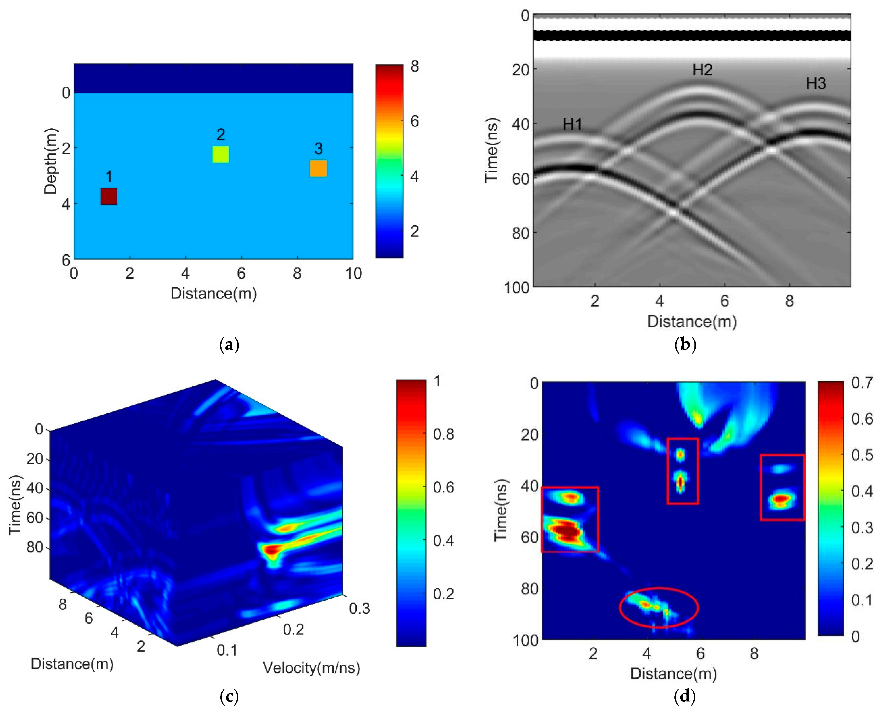
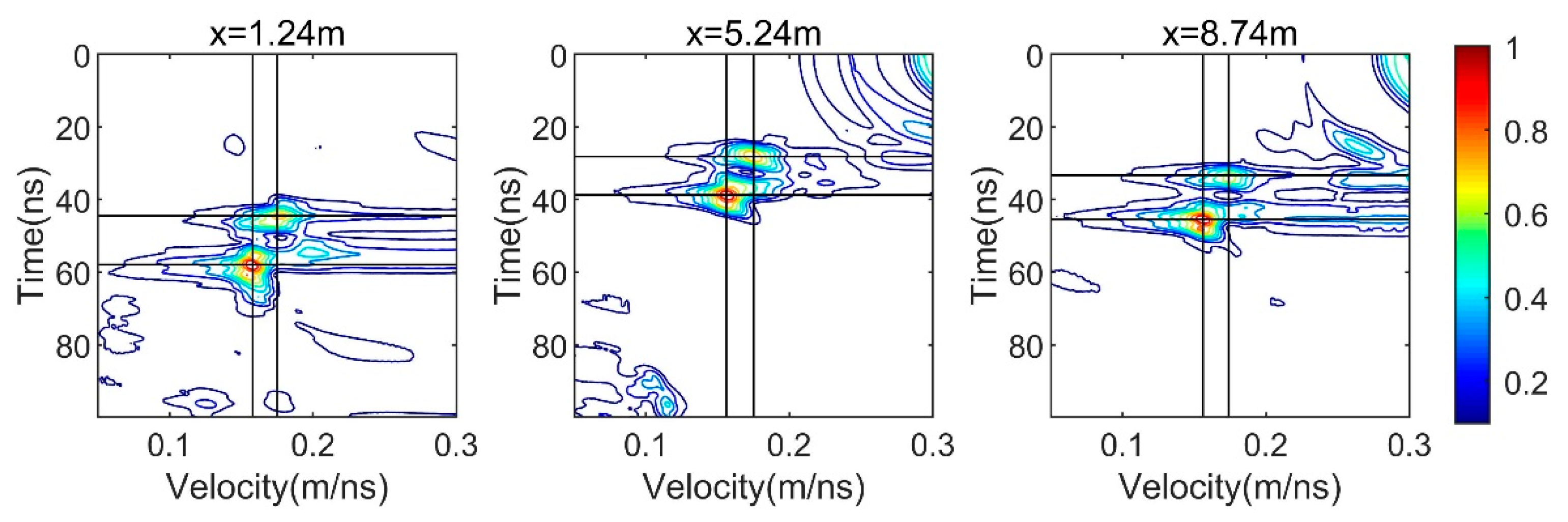
3.1. Model Test
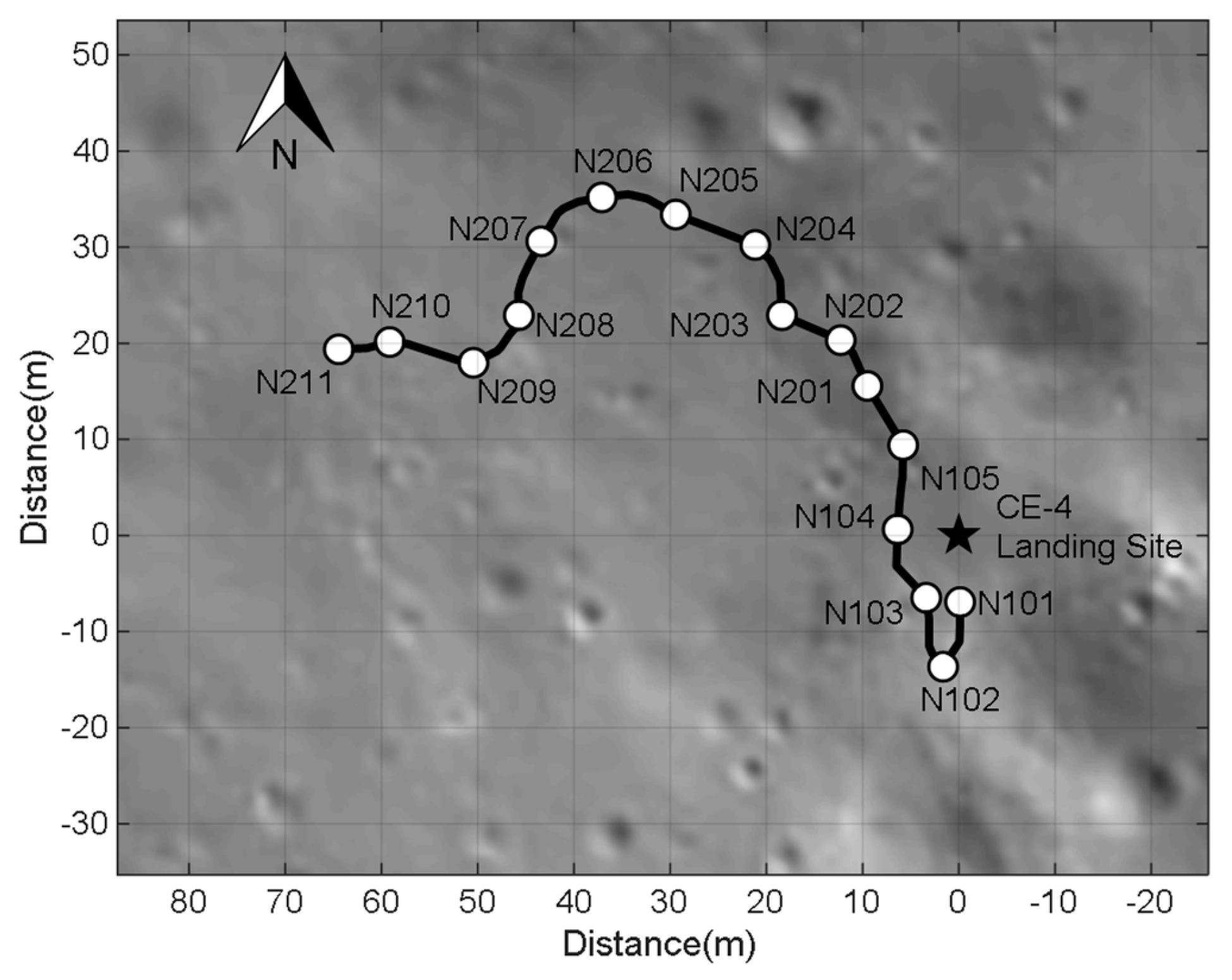
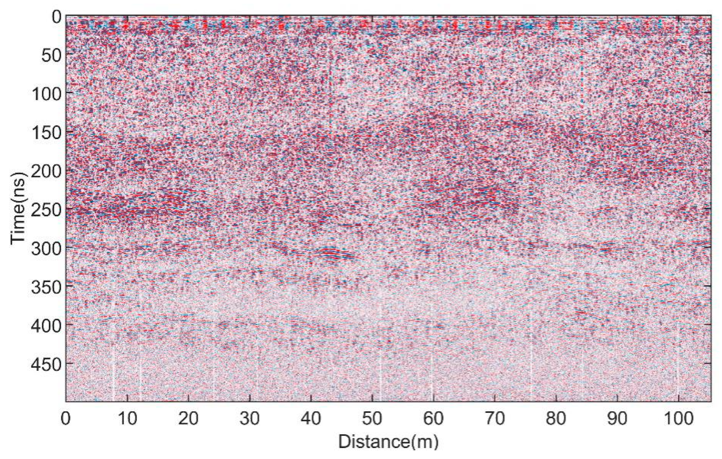
3.2. Lunar Penetrating Radar (LPR) Data Processing
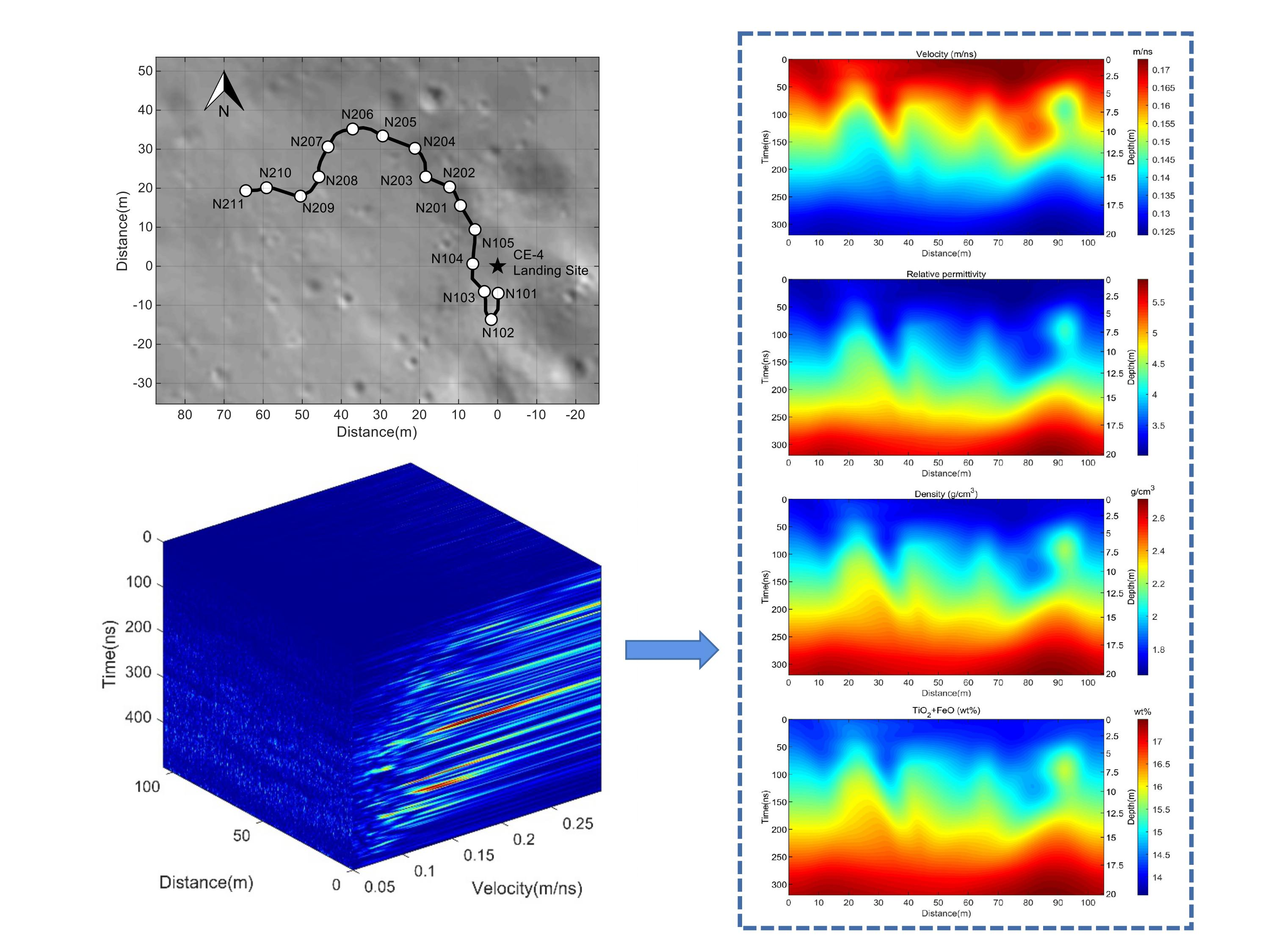
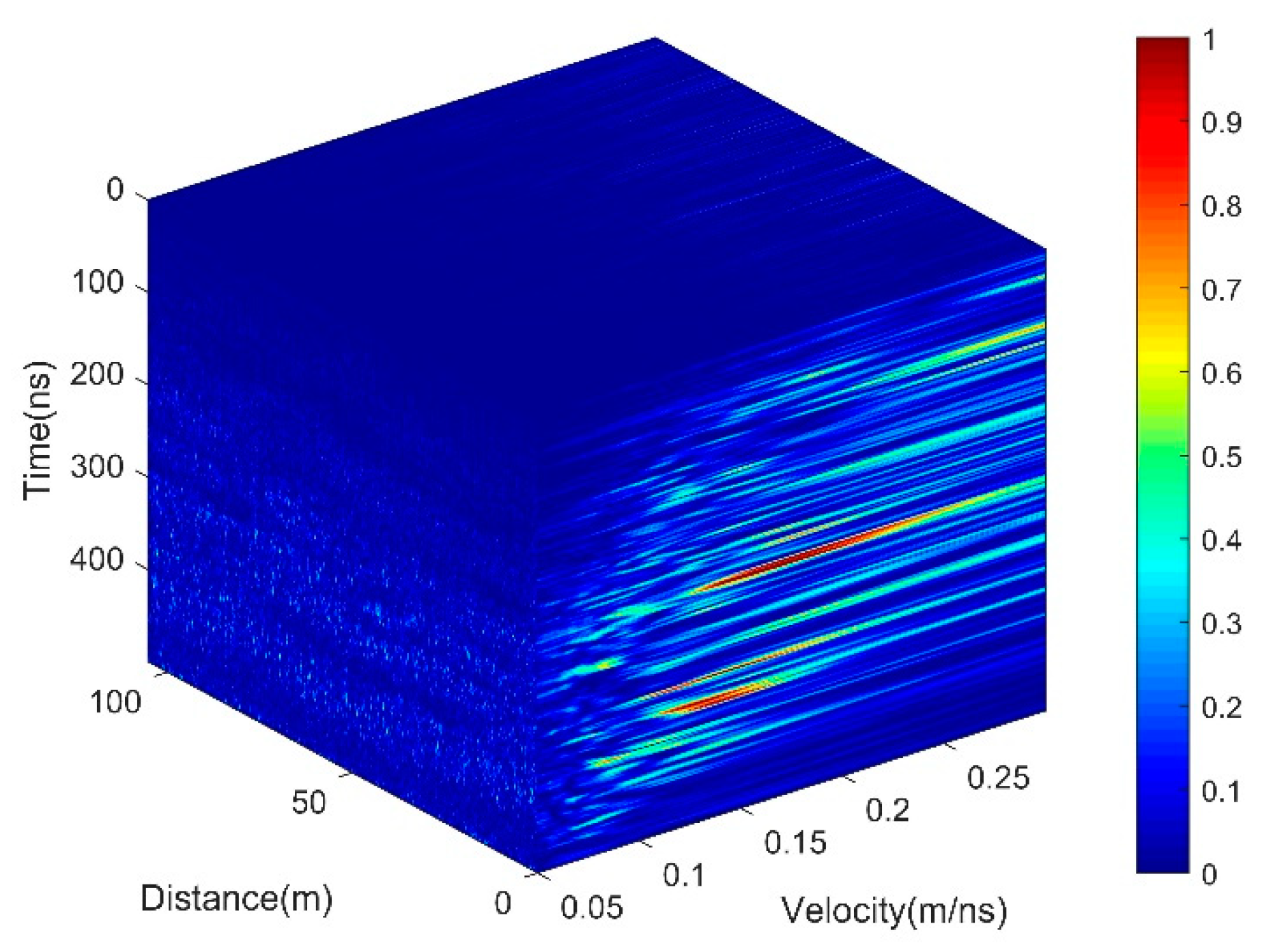
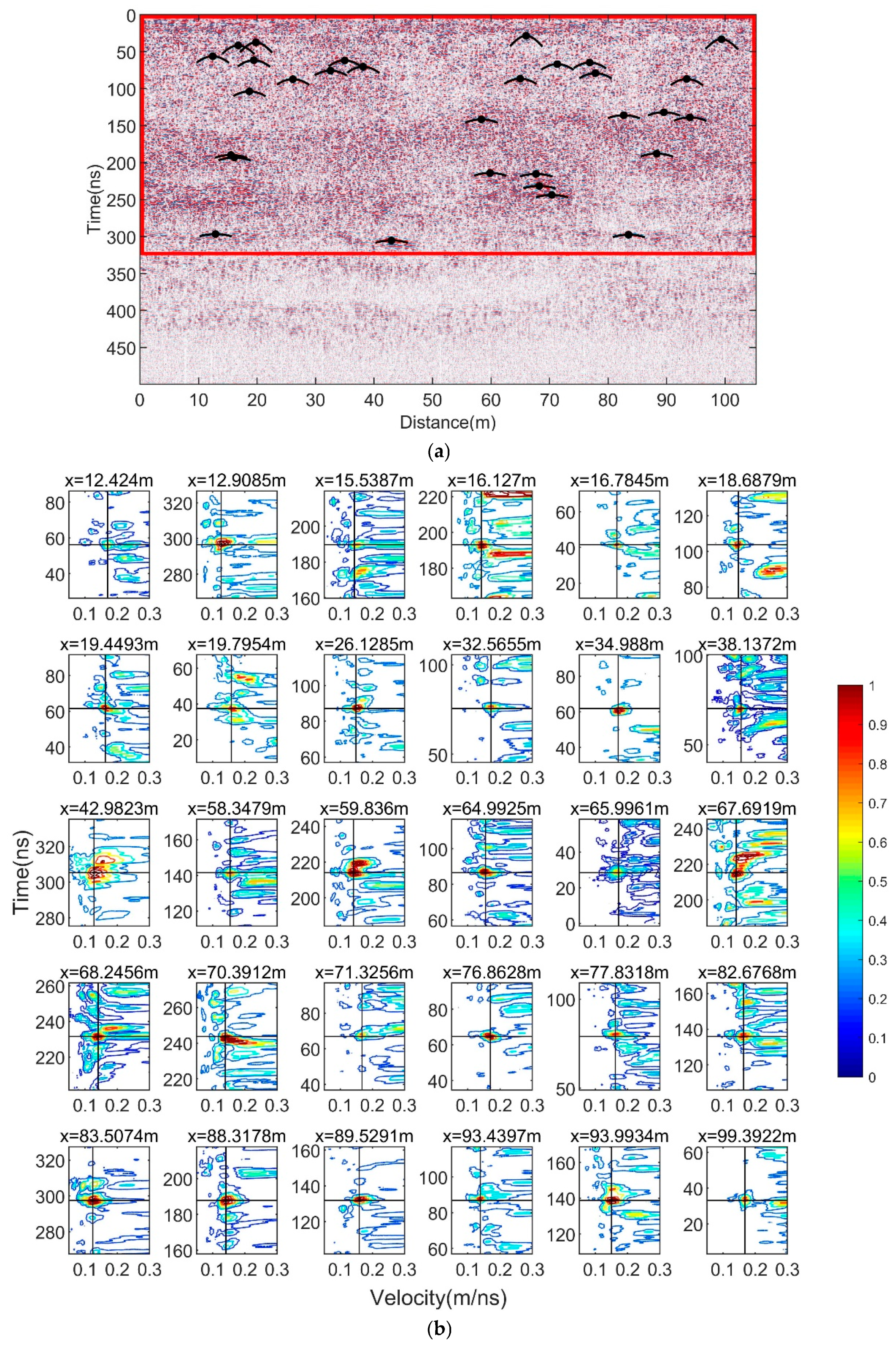
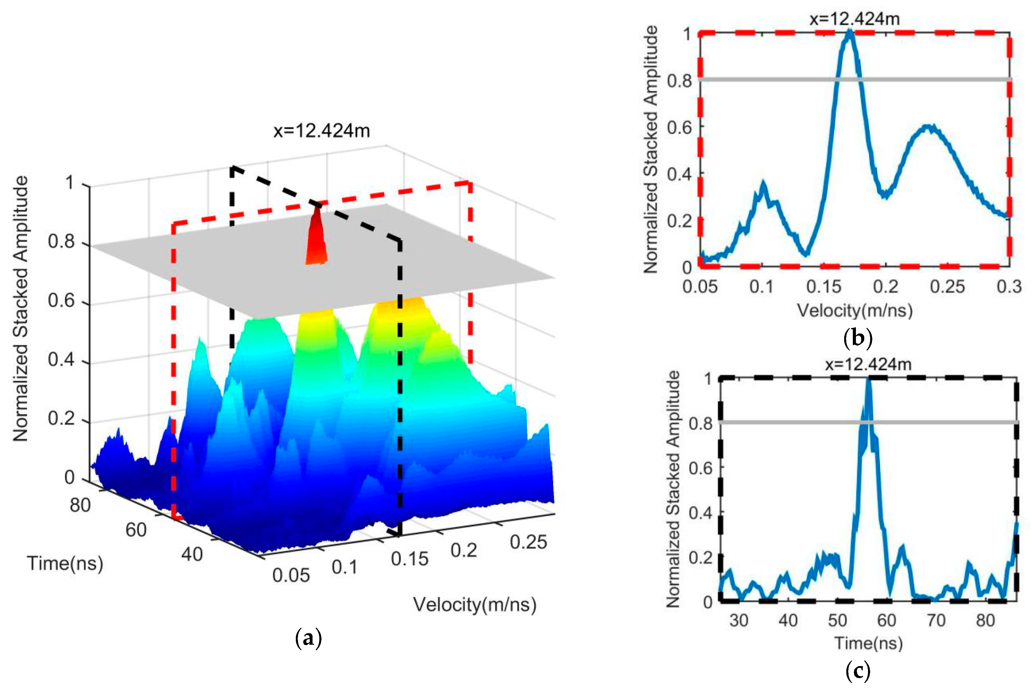
3.3. 3D Velocity Spectrum
- (1)
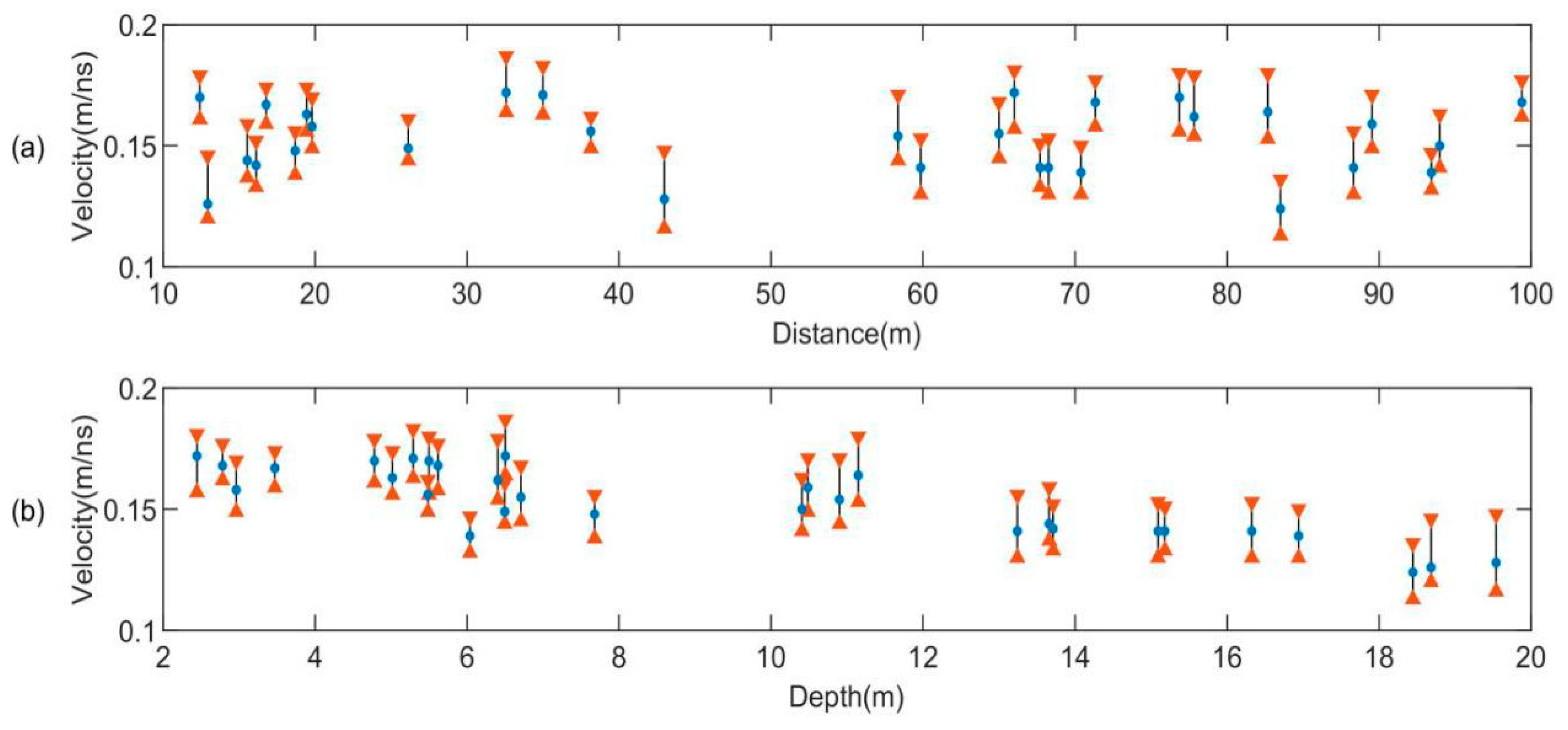
- For a highly flat interface, the estimated velocity will reach to 0.3 m/ns, which is obviously wrong; the lunar regolith velocity is less than 0.2 m/ns [24], so we delete the points with velocities close to 0.3 m/ns.
- (2)
- There may be a large stacked energy even if there are no hyperbolas but interlaced regions of several hyperbolas; for this situation, we should delete the non-hyperbolic points.
- (3)
- The hyperbolas on radargram are not curves but regions with hyperbolic shapes, so there will be several excess points at one hyperbola, which should be deleted.
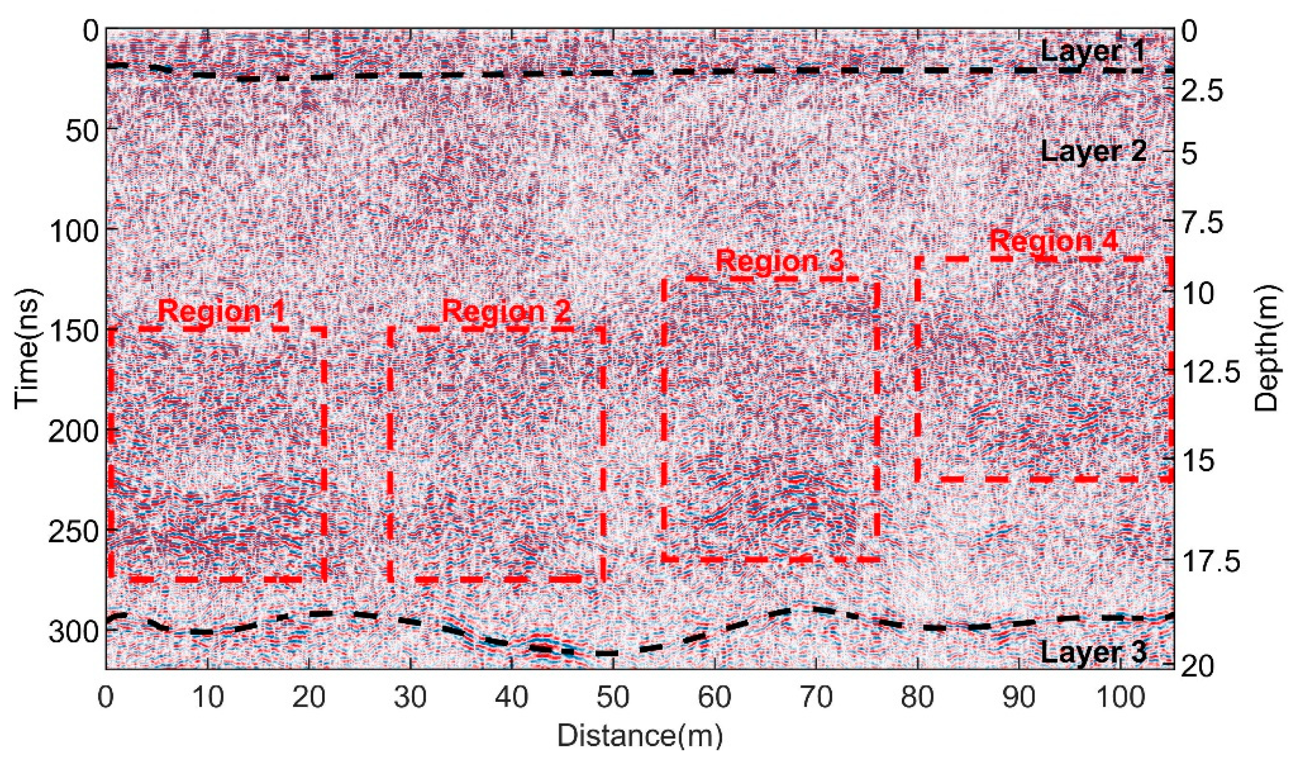
3.4. Analysis of Radargram
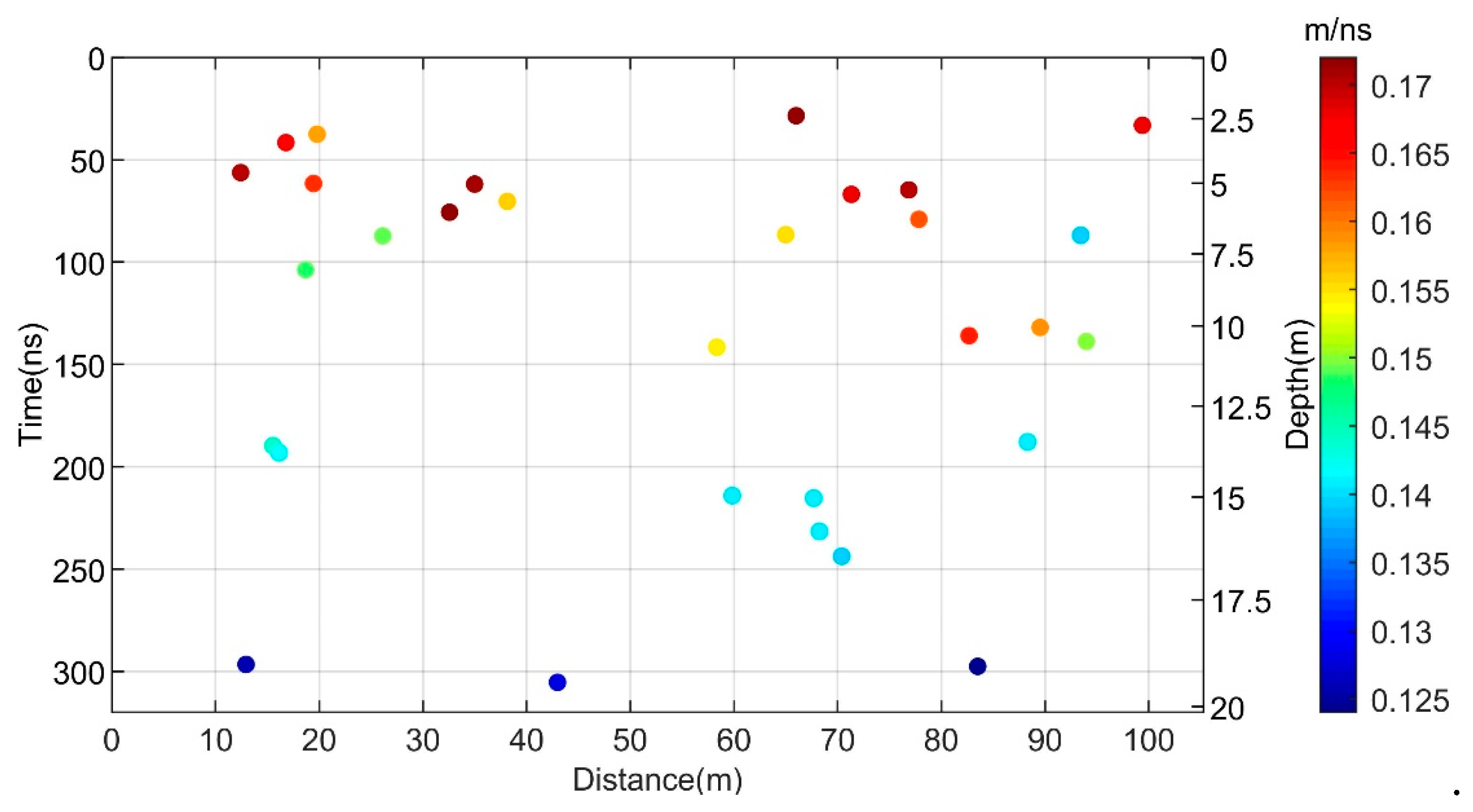
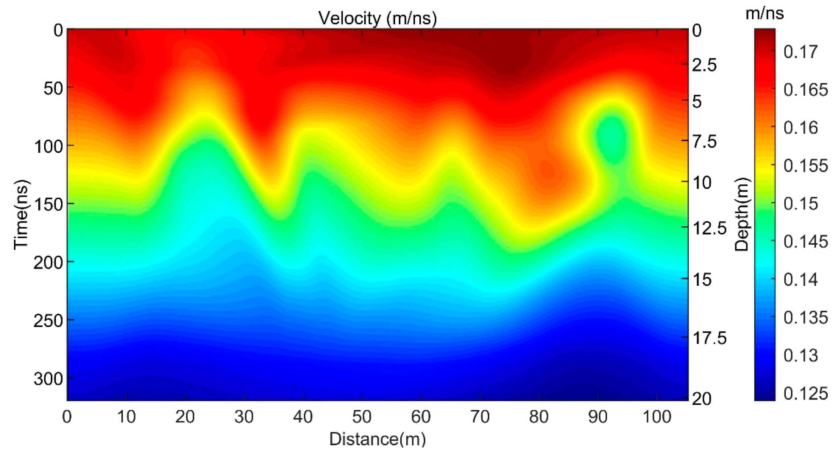
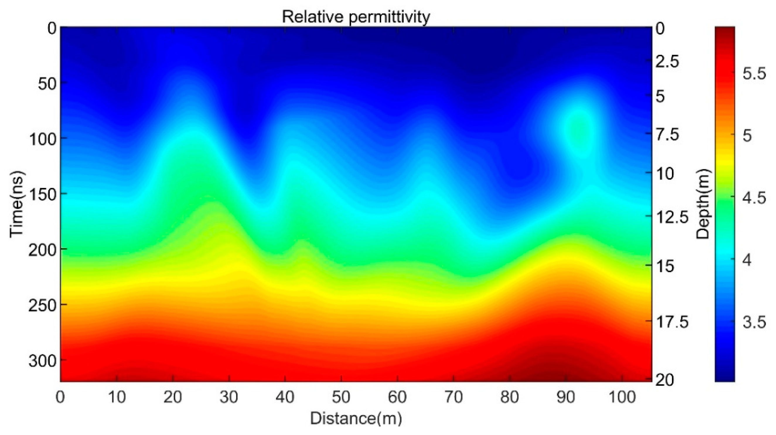
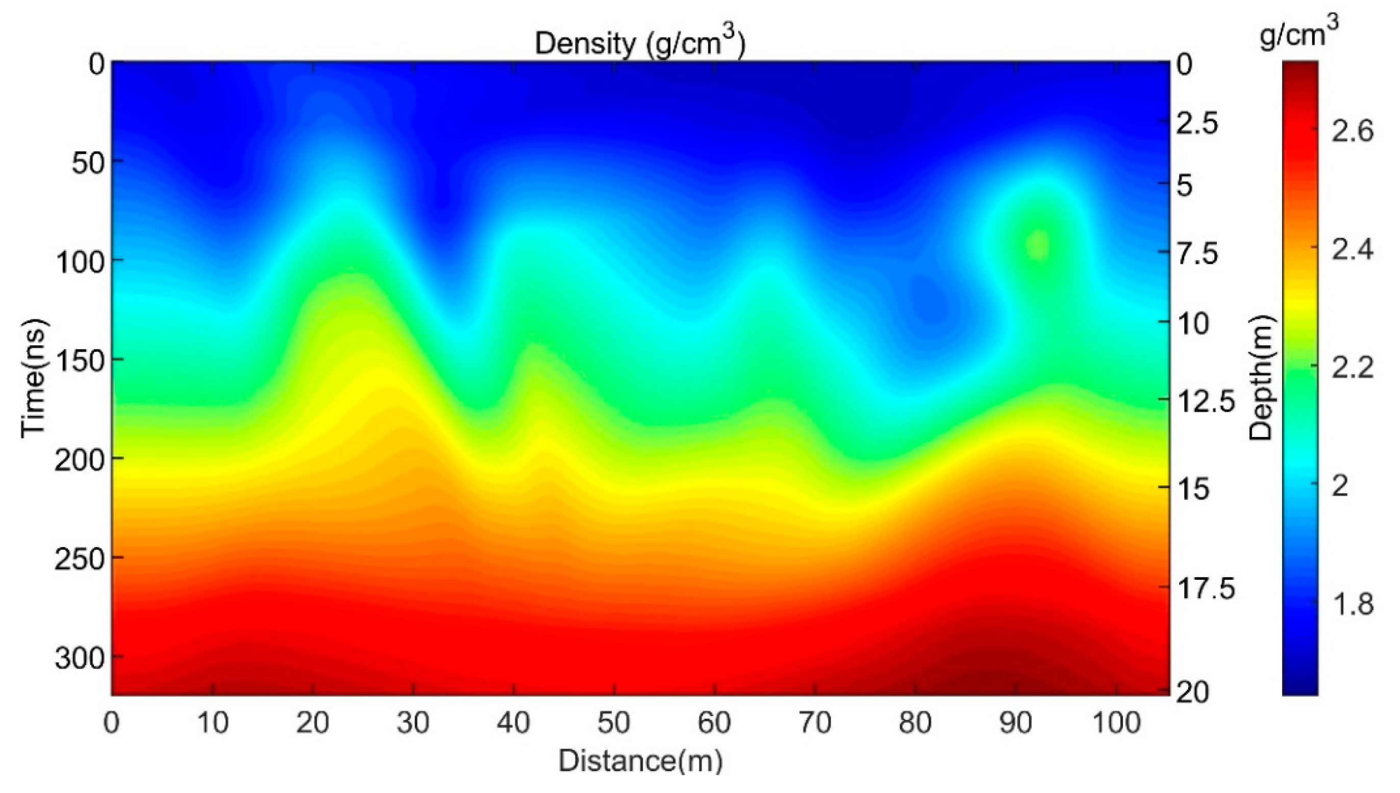
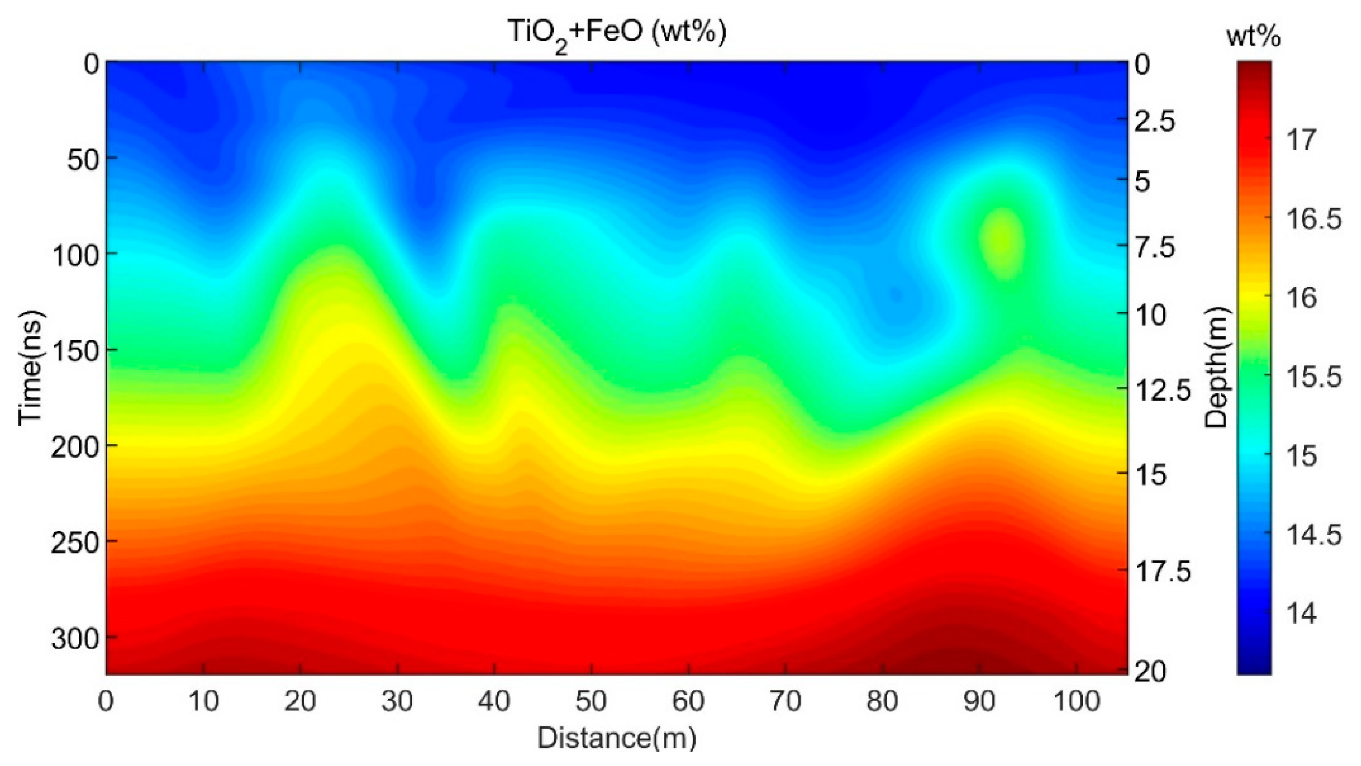
3.5. Properties Analysis
4. Discussion
5. Conclusions
Author Contributions
Funding
Conflicts of Interest
References
- Ling, Z.; Qiao, L.; Liu, C.; Cao, H.; Bi, X.; Lu, X.; Zhang, J.; Fu, X.; Li, B.; Liu, J. Composition, mineralogy and chronology of mare basalts and non-mare materials in Von Kármán crater: Landing site of the Chang’E4 mission. Planet. Space Sci. 2019, 179, 104741. [Google Scholar] [CrossRef]
- Liu, J.; Ren, X.; Yan, W.; Li, C.; Zhang, H.; Jia, Y.; Zeng, X.; Chen, W.; Gao, X.; Liu, D.; et al. Descent trajectory reconstruction and landing site positioning of Chang’E-4 on the lunar farside. Nat. Commun. 2019, 10, 4229. [Google Scholar] [CrossRef]
- Qiao, L.; Ling, Z.; Fu, X.; Li, B. Geological characterization of the Chang’e-4 landing area on the lunar farside. Icarus 2019, 333, 37–51. [Google Scholar] [CrossRef]
- Huang, J.; Xiao, Z.; Flahaut, J.; Martiont, M.; Head, J.; Xiao, X.; Xie, M.; Xiao, L. Geological characteristics of Von Kármán crater, northwestern South Pole-Aitken Basin: Chang’E-4 landing site region. J. Geophys. Res. Planets 2018, 123, 1684–1700. [Google Scholar] [CrossRef]
- Di, K.; Liu, Z.; Liu, B.; Wan, W.; Peng, M.; Li, J.; Xie, J.; Jia, M.; Niu, S.; Xin, X.; et al. Topographic Analysis of Chang’E-4 Landing Site Using Orbital, Descent and Ground Data. In Proceedings of the International Archives of the Photogrammetry, Remote Sensing and Spatial Information Sciences, Enschede, The Netherlands, 10–14 June 2019; pp. 1383–1387. [Google Scholar]
- Hu, X.; Ma, P.; Yang, Y.; Zhu, M.; Jiang, T.; Lucey, P.G.; He, Z. Mineral abundances inferred from in situ reflectance measurements of Chang’E-4 landing site in South Pole-Aitken basin. Geophys. Res. Lett. 2019, 46, 9439–9447. [Google Scholar] [CrossRef]
- Xiao, L.; Zhu, P.; Fang, G.; Xiao, Z.; Zou, Y.; Zhao, J.; Zhao, N.; Yuan, Y.; Qiao, L.; Zhang, X.; et al. A young multilayered terrane of the northern Mare Imbrium revealed by Chang’E-3 mission. Science 2015, 347, 1226–1229. [Google Scholar] [CrossRef] [PubMed]
- Fa, W.; Zhu, M.; Liu, T.; Plescia, J.B. Regolith stratigraphy at the Chang’E-3 landing site as seen by lunar penetrating radar. Geophys. Res. Lett. 2015, 42, 10,179–10,187. [Google Scholar] [CrossRef]
- Dong, Z.; Fang, G.; Ji, Y.; Gao, Y.; Wu, C.; Zhang, X. Parameters and structure of lunar regolith in Chang’E-3 landing area from lunar penetrating radar (LPR) data. Icarus 2017, 282, 40–46. [Google Scholar] [CrossRef]
- Feng, J.; Su, Y.; Ding, C.; Xing, S.; Dai, S.; Zou, Y. Dielectric properties estimation of the lunar regolith at CE-3 landing site using lunar penetrating radar data. Icarus 2017, 284, 424–430. [Google Scholar] [CrossRef]
- Su, Y.; Fang, G.; Feng, J.; Xing, S.; Jing, Y.; Zhou, B. Data processing and initial results of Chang’E-3 lunar penetrating radar. Res. Astron. Astrophys. 2014, 14, 1623–1632. [Google Scholar] [CrossRef]
- Wang, K.; Zeng, Z.; Zhang, L.; Xia, S.; Li, J. A compressive-sensing-based approach to reconstruct regolith structure from lunar penetrating radar data at the Chang’E-3 landing site. Remote Sens. 2018, 10, 1925. [Google Scholar] [CrossRef]
- Jia, Z.; Liu, S.; Zhang, L.; Hu, B.; Zhang, J. Weak Signal Extraction from Lunar Penetrating Radar Channel 1 Data Based on Local Correlation. Electronics 2019, 8, 573. [Google Scholar] [CrossRef]
- Zhang, L.; Zeng, Z.; Li, J.; Lin, J.; Hu, Y.; Wang, X.; Sun, X. Simulation of the Lunar Regolith and Lunar-Penetrating Radar Data Processing. IEEE J. Sel. Top. Appl. Earth Obs. Remote Sens. 2018, 11, 655–663. [Google Scholar] [CrossRef]
- Zhang, J.; Zeng, Z.; Zhang, L.; Lu, Q.; Wang, K. Application of Mathematical Morphological Filtering to Improve the Resolution of Chang’E-3 Lunar Penetrating Radar Data. Remote Sens. 2019, 11, 524. [Google Scholar] [CrossRef]
- Lai, J.; Xu, Y.; Zhang, X.; Tang, Z. Structural analysis of lunar subsurface with Chang’E-3 lunar penetrating radar. Planet. Space Sci. 2016, 120, 96–102. [Google Scholar] [CrossRef]
- Zhang, L.; Zeng, Z.; Li, J.; Huang, L.; Huo, Z.; Wang, K.; Zhang, J. Parameter Estimation of Lunar Regolith from Lunar Penetrating Radar Data. Sensors 2018, 18, 2907. [Google Scholar] [CrossRef] [PubMed]
- Yilmaz, Ö. Seismic Data Analysis, 3rd ed.; Society of Exploration Geophysicists: Tulsa, Oklahoma, 2001. [Google Scholar]
- Feng, X.; Sato, M. Pre-stack migration applied to GPR for landmine detection. Inverse Probl. 2004, 20, S99–S115. [Google Scholar] [CrossRef]
- Fisher, E.; McMechan, G.A.; Annan, A.P. Acquisition and processing of wide-aperture ground-penetrating radar data. Geophysics 1992, 57, 495–504. [Google Scholar] [CrossRef]
- Greaves, P.J.; Lesmes, D.P.; Lee, J.M.; Toksoz, M.N. Velocity variations and water content estimated from multi-offset, ground-penetrating radar. Geophysics 1996, 61, 683–695. [Google Scholar] [CrossRef]
- Leparoux, D.; Gibert, D.; Côte, P. Adaptation of prestack migration to multi-offset ground-penetrating radar (GPR) data. Geophys. Prospect. 2001, 49, 374–386. [Google Scholar] [CrossRef]
- Hu, B.; Wang, D.; Zhang, L.; Zeng, Z. Rock Location and Quantitative Analysis of Regolith at the Chang’e 3 Landing Site Based on Local Similarity Constraint. Remote Sens. 2019, 11, 530. [Google Scholar] [CrossRef]
- Sen, P.N.; Scala, C.; Cohen, M.H. A self-similar model for sedmentary rocks with application to the dielectric constants for fused glass beads. Geophysics 1981, 46, 781–795. [Google Scholar] [CrossRef]


| Scatters | Upper Hyperbolas | Bottom Hyperbolas | ||
|---|---|---|---|---|
| Velocity (m/ns) | Error (%) | Velocity (m/ns) | Error (%) | |
| 1 | 0.175 | 1.04 | 0.158 | 8.78 |
| 2 | 0.175 | 1.04 | 0.156 | 9.93 |
| 3 | 0.174 | 0.46 | 0.156 | 9.93 |
| Processing | Details |
|---|---|
| Traces amending | Adjusting the longitudinal displacement of traces, based on the phase of a strong reflection event |
| Traces selecting | The rover might stop at some points on the way to collect other scientific data but LPR never stops measurement, resulting in repeated acquisition of multiple traces at the same location. We average the repeated traces. |
| Time lag adjustment | There is a 28 ns delay for the start time of the transmitting antenna compared to the receiving antenna. |
| Useless data deleting | Signals after 500 ns are removed since these signals are not reliable. |
| Attenuation compensation | Conducting automatic gain control (AGC) to make deep information more visible |
| Background removal | Removing the average data along the rover path. |
| Band-pass filtering | Adopting band-pass filtering to suppress the low-frequency and high-frequency noise. |
© 2020 by the authors. Licensee MDPI, Basel, Switzerland. This article is an open access article distributed under the terms and conditions of the Creative Commons Attribution (CC BY) license (http://creativecommons.org/licenses/by/4.0/).
Share and Cite
Dong, Z.; Feng, X.; Zhou, H.; Liu, C.; Zeng, Z.; Li, J.; Liang, W. Properties Analysis of Lunar Regolith at Chang’E-4 Landing Site Based on 3D Velocity Spectrum of Lunar Penetrating Radar. Remote Sens. 2020, 12, 629. https://doi.org/10.3390/rs12040629
Dong Z, Feng X, Zhou H, Liu C, Zeng Z, Li J, Liang W. Properties Analysis of Lunar Regolith at Chang’E-4 Landing Site Based on 3D Velocity Spectrum of Lunar Penetrating Radar. Remote Sensing. 2020; 12(4):629. https://doi.org/10.3390/rs12040629
Chicago/Turabian StyleDong, Zejun, Xuan Feng, Haoqiu Zhou, Cai Liu, Zhaofa Zeng, Jing Li, and Wenjing Liang. 2020. "Properties Analysis of Lunar Regolith at Chang’E-4 Landing Site Based on 3D Velocity Spectrum of Lunar Penetrating Radar" Remote Sensing 12, no. 4: 629. https://doi.org/10.3390/rs12040629
APA StyleDong, Z., Feng, X., Zhou, H., Liu, C., Zeng, Z., Li, J., & Liang, W. (2020). Properties Analysis of Lunar Regolith at Chang’E-4 Landing Site Based on 3D Velocity Spectrum of Lunar Penetrating Radar. Remote Sensing, 12(4), 629. https://doi.org/10.3390/rs12040629