Consistency of Radiometric Satellite Data over Lakes and Coastal Waters with Local Field Measurements

Abstract

The Sentinel-3 mission launched its first satellite Sentinel-3A in 2016 to be followed by Sentinel-3B and Sentinel-3C to provide long-term operational measurements over Earth. Sentinel-3A and 3B are in full operational status, allowing global coverage in less than two days, usable to monitor optical water quality and provide data for environmental studies. However, due to limited ground truth data, the product quality has not yet been analyzed in detail with the fiducial reference measurement (FRM) dataset. Here, we use the fully characterized ground truth FRM dataset for validating Sentinel-3A Ocean and Land Colour Instrument (OLCI) radiometric products over optically complex Estonian inland waters and Baltic Sea coastal areas. As consistency between satellite and local data depends on uncertainty in field measurements, filtering of the in situ data has been made based on the uncertainty for the final comparison. We have compared various atmospheric correction methods and found POLYMER (POLYnomial-based algorithm applied to MERIS) to be most suitable for optically complex waters under study in terms of product accuracy, amount of usable data and also being least influenced by the adjacency effect.

1. Introduction

There is a growing constellation of satellite sensors providing Earth observation data for monitoring aquatic ecosystems. These ecosystems provide complex conditions for optical remote sensing in terms of optical water types. The adjacency to land also causes bias due to multiple scattering of the light detected by the sensor [1] which needs to be removed when the aim is to detect optical properties of the water.

Sentinel-3 (S3) is an ocean and land mission that consists of three satellites S3A, S3B and S3C, providing environmental monitoring data under the Copernicus program until 2030 [2,3]. There are four different instruments onboard S3 satellites, from which Ocean and Land Colour Instrument (OLCI) is a medium-resolution imaging spectrometer aimed for monitoring optical water quality. OLCI fulfills many of the mission objectives, e.g., measuring ocean and land surface color, monitoring seawater quality and pollution and monitoring land use change. OLCI is also the main contributor to monitoring inland waters [4]. One of the S3 mission requirements is that the measurements and products shall include uncertainty estimates [4]. The uncertainties shall be within 5% for the radiometric data. Currently in OLCI-A open water products, the water-leaving reflectance $\lfloor {\rho }_w\rfloor {}_N$ partly meets the S3 mission requirements at averaged global and temporal scales [5] where bands at 490, 510 and 560 nm are within the 5% mission requirement uncertainty for all water types; bands 400, 412 and 442 are within 5–10% depending on water type and bands at longer wavelengths having uncertainties higher or depending on a water type. OLCI-A Level-2 Ocean Colour (OC) operational products provide additional per-pixel uncertainty estimates but they have not been verified yet as they do not include uncertainty estimate from the Level-1 products [2]. In parallel, active research is ongoing to better quantify in situ measurement uncertainties in controlled (laboratory) [6] and in natural measurement (outdoors) [7] conditions. This enables collecting fiducial reference measurements (FRM) that are traceable to SI standards and can be further used with confidence for the validation of satellite products. This FRM data improves the comparability of radiometric in situ measurements with ocean color data, e.g., S3 OLCI data to analyze the performance of the algorithms, estimate the errors and characterize the main sources of uncertainties.

From the S3 OLCI constellation, both S3 A and B are on-orbit and provide daily measurements. The products of S3 A and B OLCI sensor are slightly different due to (1) instrument radiometric response; (2) system vicarious calibration; (3) modeling of the temporal evolution at Level-1 products; (4) spectral response functions; (5) radiometric and geometric behaviors of both instruments [2]. In this study, we focused solely on S3A OLCI products to exclude conclusions based on the differences between the sensors and their data processing.

The objectives of this work are: (1) to analyze the in situ measured radiometric data in order to find the sources and variability of uncertainties; (2) to provide uncertainty budgets for in situ datasets which can be used to reveal and explain differences with the S3A OLCI data over optically complex waters; and (3) to identify the most suitable atmospheric correction (AC) algorithm.

2. Materials and Methods

2.1. Study Sites

Field measurements were carried out in large Estonian lakes Peipsi and Võrtsjärv and in Baltic Sea coastal waters (

Table 1. Morpho-dynamical data and bio-optical parameters of the study sites (minimum, maximum and median value).

Parameter	Lake Peipsi	Lake Võrtsjärv	Baltic Sea Coastal
Mean depth, m	7	2.8	7.5
Max depth, m	15.3	6	12
Chla, mg·m−3	2.7–122 (25.1)	3.4–72.2 (40.4)	0.7–10.7 (4.1)
CTSM, g·m−3	1.3–61.3 (8.8)	1.6–52.7 (16)	5.0–24.3 (10)
aCDOM (442), m−1	1.2–7 (2.9)	1.9–8.9 (2.9)	0.6–3.7 (0.9)
Secchi depth, m	0.4–3.6 (1.5)	0.2–2.6 (0.75)	0.5–4.3 (1.3)

Note: TSM: total suspended matter; a_CDOM: absorption coefficient of colored dissolved organic matter at 442 nm; Chla: chlorophyll-a.

). Lake Peipsi and Võrtsjärv are large, shallow and well-mixed Estonian lakes. Lake Peipsi is a transboundary waterbody between Russia and Estonia. It is divided into three parts: in the north mesotrophic Lake Peipsi sensu stricto (s.s.), in the south hypertrophic Lake Pihkva and their connection and river-like eutrophic Lämmijärv. Different water types can be observed in this lake: clearest and deepest water in Peipsi s.s., turbid and brownish water near the river Suur Emajõgi delta and phytoplankton rich Lämmijärv and L. Pihkva. In the summertime, cyanobacterial blooms may be present in the entire lake. Lake Võrtsjärv is a very turbid, well-mixed, eutrophic and non-stratified lake with a high absorption coefficient of colored dissolved organic matter at wavelength 442 nm (a_CDOM), phytoplankton and concentration of total suspended matter (TSM). Water level variations control nutrient and phytoplankton availability. The Baltic Sea is a semi-enclosed sea with relatively high freshwater input by rivers. The ranges of the optical parameters over the Baltic Sea areas are wide [8], and a_CDOM is the dominant optical component [9] with a strong relationship with salinity [10].

2.2. In Situ Measurements

The above-water radiometric measurements were performed from the research vessel (approximately 6 m long) from about 2 m height from the water surface. In each station, the vessel was anchored and radiometric measurements were recorded at least for 15 min. The water-leaving reflectance spectra were calculated from the well-synchronized time series measured with the three above water TriOS-RAMSES hyperspectral radiometers following the protocol of REVAMP [11]. Calculations included the following steps: firstly, all measured radiance and irradiance spectra were corrected for the stray light [6,12]; secondly, spectral response functions of OLCI bands were used to convolve spectra into OLCI band values; thirdly, the time series of water-leaving reflectance $\lfloor {\rho }_w\rfloor {}_N$ was calculated as

$$\lfloor {\rho }_w\rfloor {}_N=\pi R_{rs}\left(\lambda \right)=\pi \frac{L_u\left(\lambda \right)-\rho \left(W\right)L_d\left(\lambda \right)}{E_d\left(\lambda \right)}$$

(1)

where $R_{rs}\left(\mathsf{\lambda }\right)$ is the remote sensing reflectance, $L_u\left(\lambda \right)$ is the upwelling radiance from the sea, $L_d\left(\lambda \right)$ is the downwelling radiance from the sky, $E_d\left(\lambda \right)$ is the downwelling irradiance and $\rho \left(W\right)$ is the sea surface reflectance as function of wind speed ($W$, m·s⁻¹), calculated as

$$\rho \left(W\right)=0.0256+0.00039W+0.000034W^2$$

(2)

[11]. Next, the Near-Infrared (NIR) similarity correction with λ₁ = 720 nm, λ₂ = 780 nm and α = 2.35 was applied to the water-leaving reflectance according to Ruddick et al. [13]. The constant parameter α of the NIR similarity correction [14] is determined in [13] and depends on the choice of wavelengths λ₁ and λ₂; α = 2.35 for the λ₁ = 720 nm and λ₂ = 780 nm.

After that, for each measurement station, the median of $R_{rs}\left(560\right)$ (OLCI band value with center at 560 nm) was calculated. Any spectrum deviating from the mode more than ±10% was excluded from further analysis in order to eliminate outliers due to changing measurement and illumination conditions. Finally, the mean water-leaving reflectance with uncertainty [15] was calculated to each measurement station.

Additionally, environmental parameters such as wind speed, cloudiness, sun condition, solar elevation angle, wave height, Secchi depth and concentrations of optically significant constituents (OSC, e.g., concentration of chlorophyll-a, concentration of total suspended matter and absorption coefficient of colored dissolved organic matter at wavelength 442 nm) were measured. The wind speed was measured with a handheld mechanical anemometer. The overall sky cloudiness, the presence of clouds in front of the sun and the wave height were estimated by visual inspection. For cloudiness, a 100-point scale was used with 0 for clear sky to 100 for fully covered. Sun condition was classified into four groups: clear, partially covered, through optically thin clouds and fully covered. For Secchi depth, the white disk with 30 cm diameter was used and measurements were performed on the shaded side of the vessel. The solar elevation angle was calculated based on the measurements time and geographic coordinates. For concentrations of OSC, the water samples were collected from the water surface (up to 0.5 m depth) and analyzed using the methods of Lindell et al. [16]. Chlorophyll-a (Chl a) was measured spectrophotometrically with a Hitachi U-3010 spectrophotometer and calculated according to the method of Jeffrey and Humphrey [17]. TSM was measured gravimetrically. Lastly, a_CDOM(442) was derived by water sample filtering through a filter with a pore size of 0.2 µm and measured in a 5 cm optical cuvette against distilled water with a Hitachi U-3010 spectrophotometer.

2.3. Uncertainty Budget

The methodology used for the uncertainty evaluation is consistent with the ISO Guide to the Expression of Uncertainty in Measurement (GUM) [18]. The evaluation is based on the measurement model, which describes the output quantity Y as a function f of input quantities X_i: Y = f(X₁, X₂, X₃, …). For example, for remote sensing reflectance R_rs(λ), Equations (1) and (2) are used. For every input quantity X_i, respectively, estimate x_i and standard uncertainty u(x_i) are evaluated which are considered as parameters of probability distribution describing the X_i. The combined standard uncertainty u_c(y) for output estimate is calculated from the standard uncertainties associated with each input estimate x_i, using a first-order Taylor series of y = f(x₁, x₂, x₃, …). There are two types of standard uncertainties: Type A is of statistical origin; Type B is determined by other means. Both types of uncertainties are indicated as standard deviation, denoted correspondingly by s and u. In calibration of array spectrometers, the uncertainty contributions arising from averaging of a large number of repeatedly measured spectra is considered as of Type A. Contributions from calibration certificates (standard lamp, diffuse reflectance panel, multimeter, current shunt, etc.), but also from instability and spatial non-uniformity of the lamp are considered for Type B.

Radiometric calibration of the irradiance and radiance sensors and their uncertainty budgets are described in [19]. The uncertainty of radiometric calibration stated in [19] has been successfully verified in international comparison between four participants (Tartu observatory of University of Tartu, National Physical Laboratory, The Joint Research Centre, TriOS) in 2016, and since 2018, respective calibration services are accredited by Estonian Accreditation Centre (EAK). Information about the use of calibrated sensors for laboratory and field measurements, about the evaluation of corrections due to different effects and/or respective uncertainty contributions without corrections applied are given in [6,7]. Additional information about the long-time instability of sensors can also be found in [6].

In the three-radiometer system used for the determination of R_rs(λ) in this paper, the same standard lamp was used for the calibration of all three sensors measuring, respectively, Ed, Lu and Ld. Therefore, the system calibration accounts for mechanical alignment of the lamp, plaque and sensors, for inadequate baffling, only for the short time instability of the irradiance standard, and for the uncertainty of the diffuse reflectance plaque. The contribution of the lamp calibration uncertainty cancels almost fully out.

The following components were included to the uncertainty budget of the in situ R_rs(λ): radiometric calibration of the three-radiometer system, responsivity drift of sensors after calibration, temperature effects, interpolation to the common wavelength scale, angular response of the irradiance sensor, wind speed uncertainty, uncertainty in the stray light correction and contribution due to polarization effects (all Type B estimates), repeatability of recorded time series, corrected for lag-1 autocorrelation and uncertainty in the NIR similarity correction (both Type A estimates).

Due to the unstable nature of natural illumination in individual time series recorded during field measurements, often a rather strong autocorrelation was visible. Consequently, besides white noise, a relatively high contribution of 1/f type noise can be expected, and the effective number of repetitions will be substantially reduced. Thus, in this case, the effective number of independent measurements has to be considered instead of actual number of data points in the recorded series [20]:

$$n_e\approx n_t\frac{1-r_1}{1+r_1}$$

(3)

where r₁ is the lag-1 autocorrelation coefficient of the analyzed time series.

If the averaged values of different radiometers are used in calculations, then due to these random drifts in time series, zero correlation between the signals of different radiometers cannot be expected, and respective correlations shall always be estimated and accounted for. The calculation scheme of R_rs(λ) used in this article is based on example H2.4 of (ISO GUM) [18], where the output time series is determined from three sets of simultaneously obtained observations. By using this approach, the combined uncertainty of R_rs(λ) is estimated from the time series of R_rs(λ) output spectra, and the evaluation of correlations between input quantities is not needed. As the values of the time series are statistically dependent, for uncertainty of the averaged value, the effective sample size is calculated by using Equation (3). NIR similarity correction is calculated for every spectrum of water-leaving reflectance ⌊ρw⌋_N, and then as the average of these values. For uncertainty of the averaged NIR similarity correction value, the effective sample size estimated from Equation (3) has also been used.

Finally, the spectra of the relative uncertainty components were convolved to the OLCI band values used for comparison.

2.4. Atmospheric Correction Processors for OLCI Data

S3A OLCI L1 and L2 Full Resolution Non Time Critical data were downloaded from databases CODAREP (period 2016–2017, baseline 2.23) and CODA (2018, baseline 2.42). Same-day match-ups were used and the distance from the shoreline and the time difference between the satellite overpass and in situ measurements were derived. A 1 × 1 pixel area was used as a satellite match-up point.

L1 data were processed with AC processors POLYMER (v4.10), Case 2 Regional CoastColor (C2RCC) Processor (v1) and Alternative Neural Net (v1) using SNAP (v6) software developed by Brockmann Consult, Array Systems Computing and Communication and Systémes (C-S).

S3 OLCI L1 are geo-located top-of-atmosphere radiance products, which have passed quality checks and radiometric calibration with pixel classification, correction for atmospheric gasses and smile effect correction. S3 OLCI L2 are atmospherically corrected products produced by using two different AC methods (Baseline Atmospheric Correction (BAC) and Alternative Atmospheric Correction) in parallel for ensuring similarity and consistency to MERIS products. BAC is based on previously developed AC for MERIS [21], which includes also a Bright Pixel Correction [22]. BAC is based on a coupled atmosphere–hydrological model using spectral optimization inversion for outputting water-leaving reflectances. It includes sun glint and white gaps correction, which is determined by certain thresholds for glint detection on a pixel. For detecting the correct band for further AC procedure, Case 2 NIR reflectance estimation process is performed based on radiometry, which includes aerosol and Rayleigh correction. Uncertainties of L1 and L2 products do not contain the full uncertainty budget at the moment, therefore these are suggested by the developers only for qualitative analyses [23]. Quality control was done by excluding pixels flagged as: WQSF_lsb_CLOUD, WQSF_lsb_CLOUD_AMBIGUOUS, WQSF_lsb_CLOUD_MARGIN, WQSF_lsb_COSMETIC, WQSF_lsb_SUSPECT, WQSF_lsb_HISOLZEN, WQSF_lsb_SATURATED, WQSF_lsb_HIGHGLINT, WQSF_lsb_OCNN_FAIL, WQSF_lsb_AC_FAIL and including flagged as WQSF_lsb_BPAC_ON.

POLYMER (POLYnomial-based algorithm applied previously to MERIS) is an AC processor originally developed for MERIS products to remove the sun glint effects of ocean waters, however further development made it applicable to optically complex waters. The AC procedure uses a spectral matching method based on polynomial the atmospheric model and bio-optical water reflectance model, which use all the spectral bands in the visible spectrum. The models are adjusted to obtain the best spectral fit for optimizing the parameters into both models. Unlike other AC processors, POLYMER is based only on NIR bands, which makes the processor able to derive the water-leaving reflectance in the presence of sun glint. For processing the data for the analysis, default parameters were used [24,25]. Quality control was done by including pixels where layer “Bitmask” had values 0 and 1024.

Case 2 Regional CoastColor (C2RCC), originally developed by Doerffer and Schiller [26], is an atmospheric correction processor for optically complex Case 2 waters, which is trained and able to work in extreme conditions of scattering and absorption. It is based on inversion by the neural network technology, which uses a large database of radiative transfer simulations of water-leaving reflectance and top-of-the-atmosphere TOA radiances, taking into account certain water parameters (temperature, salinity) and atmospheric conditions (ozone, air pressure) [27]. For processing the data for the analysis, default parameters (except salinity for inland waters 0.0001) were used. Alternative Neural Net (ALTNN) is a combined AC processor of C2RCC and Case-2 Extreme. Alternative Neural Net is based on the same neural network system as C2RCC, but it has been improved and revised for more accurate results. It is a test version for OLCI and MERIS data with an extended training range and a larger number of training samples, which reduces noise in results and the gives opportunity to derive more reliable results [27]. For both C2RCC and ALTNN, the pixels were excluded from the analyses, which were flagged as: Rhow_OOS, Cloud_risk, Rhow_OOR, Rtosa_OOR, Rtosa_OOS, quality_flags_sun_glint_risk.

2.5. Data Analysis

First, the in situ dataset was analyzed with Principal Component Analysis (PCA) to visualize the variation present in the in situ radiometric dataset in relation to the uncertainty budget. PCA analyses were performed with R software using the ggbiplot package and prcomp function. Inputs for the PCA were the concentrations of (1) Chl a (mg·m⁻³), (2) TSM (g·m⁻³), (3) a_CDOM(442) (m⁻¹), (4) wind speed (m·s⁻¹), (5) cloudiness (from 0 to 100), (6) Secchi depth (m), (7) solar elevation angle (degree), (8) R_rs at 560 (sr⁻¹), (9) wave height (m), (10) presence of clouds in front of the sun in the scale of 1–4 (1, clear; 2, fully covered; 3, through a thin cloud; 4, partially covered).

Second, the accuracy of the satellite-derived Remote Sensing Reflectance $R_{rs}{\left(\lambda \right)}_{olci,i}$ was then compared against the in situ measured $R_{rs}{\left(\lambda \right)}_{insitu,i}$ values. Mean Absolute Percentage Difference (MAPD) was applied to investigate dispersion and Mean Percentage Difference (MPD) to investigate bias:

$$MAP{D}_{\lambda }=\frac{{{\displaystyle \sum }}_{i=1}^{n}100\left|\frac{R_{rs}{\left(\lambda \right)}_{olci,i}-R_{rs}{\left(\lambda \right)}_{insitu,i}}{R_{rs}{\left(\lambda \right)}_{insitu,i}}\right|}{n}$$

(4)

$$MP{D}_{\lambda }=\frac{{{\displaystyle \sum }}_{i=1}^{n}100\left(\frac{R_{rs}{\left(\lambda \right)}_{olci,i}-R_{rs}{\left(\lambda \right)}_{insitu,i}}{R_{rs}{\left(\lambda \right)}_{insitu,i}}\right)}{n}$$

(5)

Here, $R_{rs}{\left(\lambda \right)}_{insitu,i}$ and $R_{rs}{\left(\lambda \right)}_{olci,i}$ are, respectively, in situ and OLCI-derived values for the band λ and match-up i.

3. Results

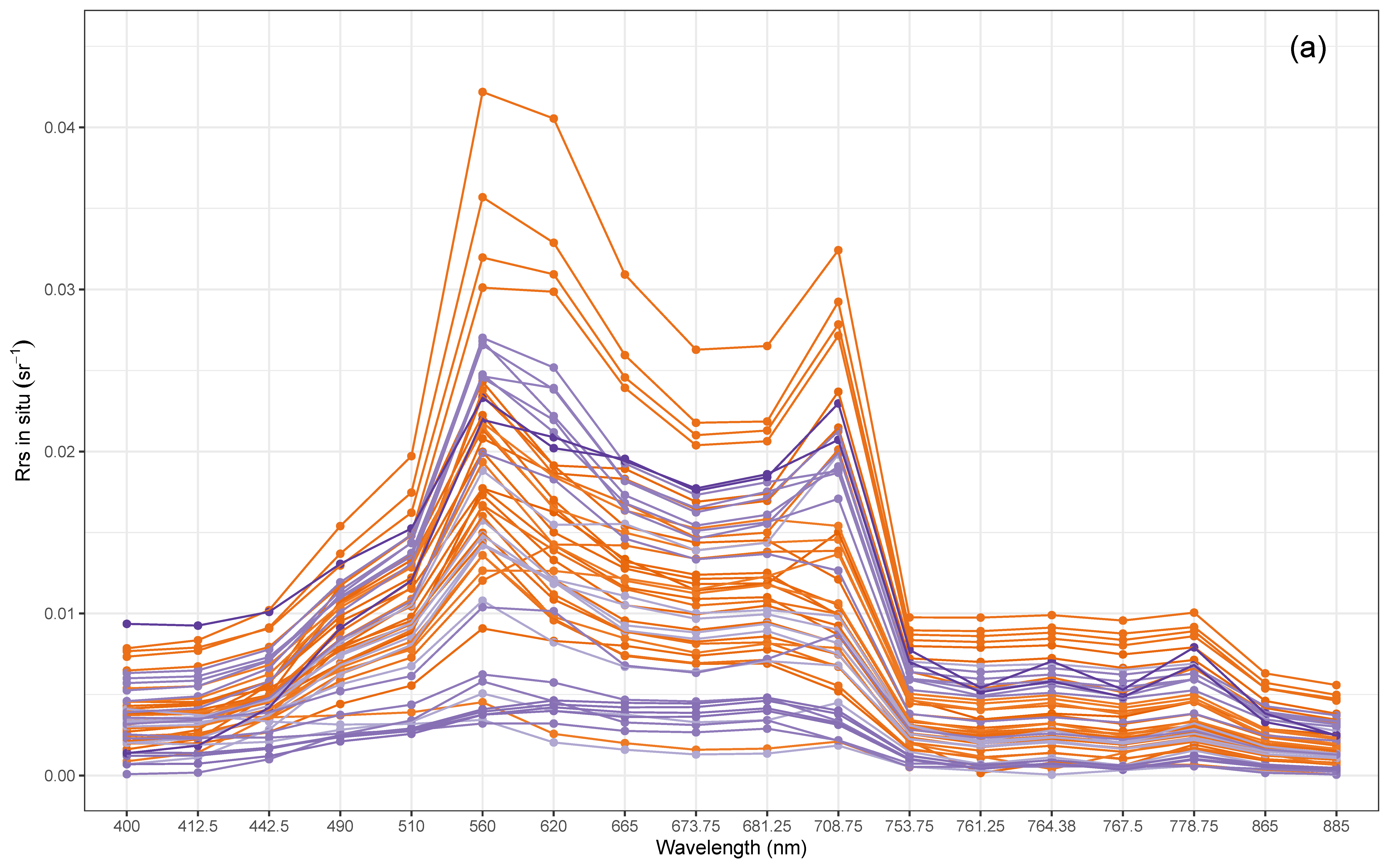
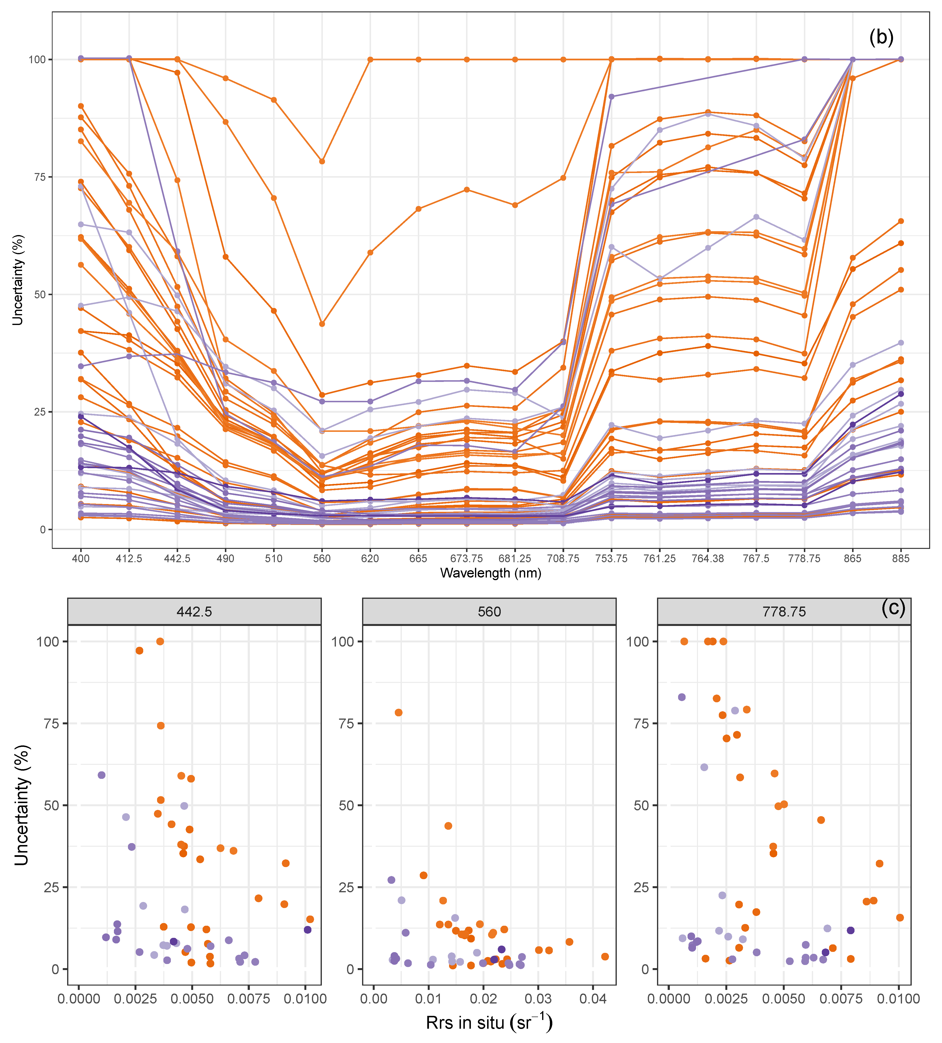
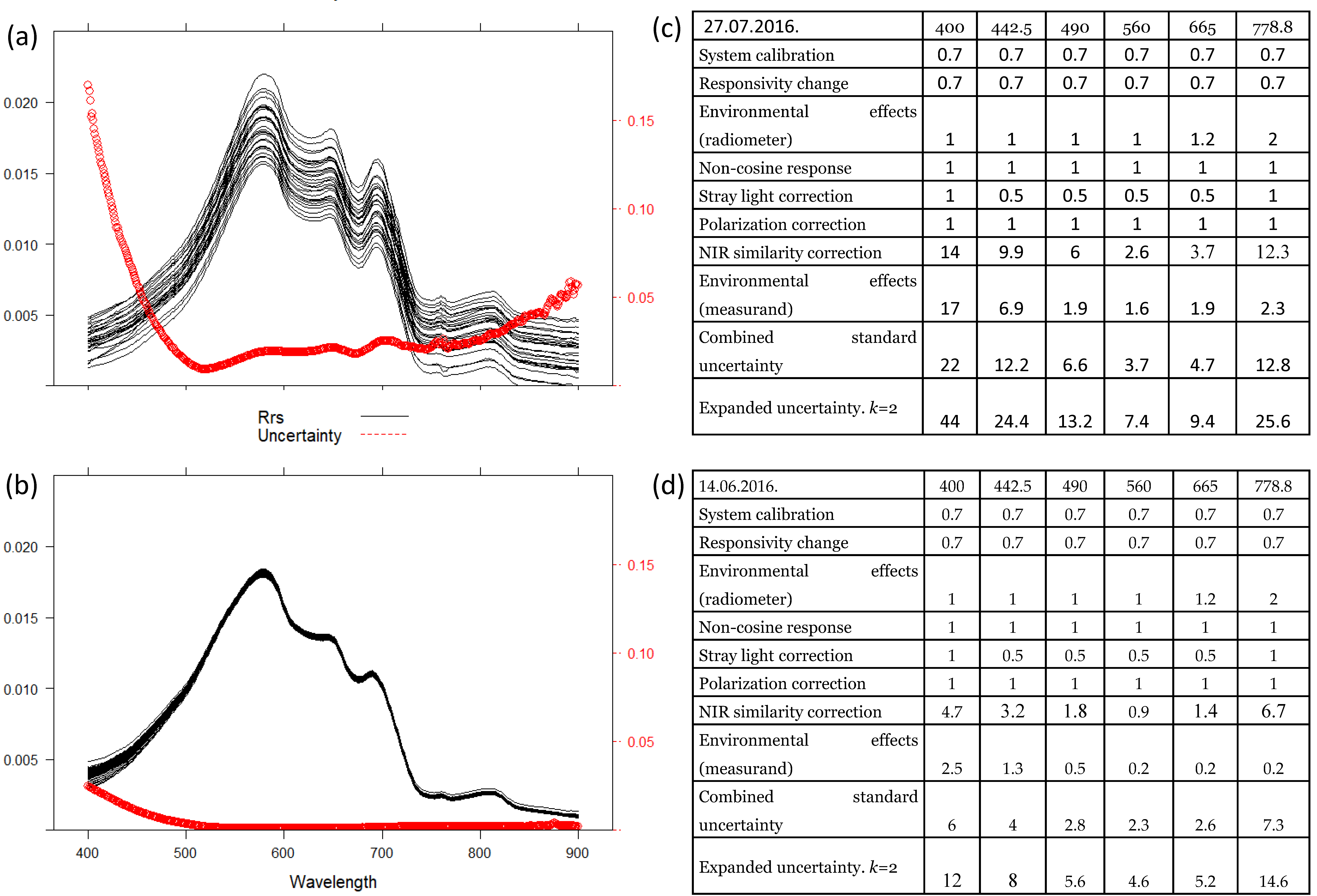
3.1. In Situ Dataset in Terms of Associated Uncertainties

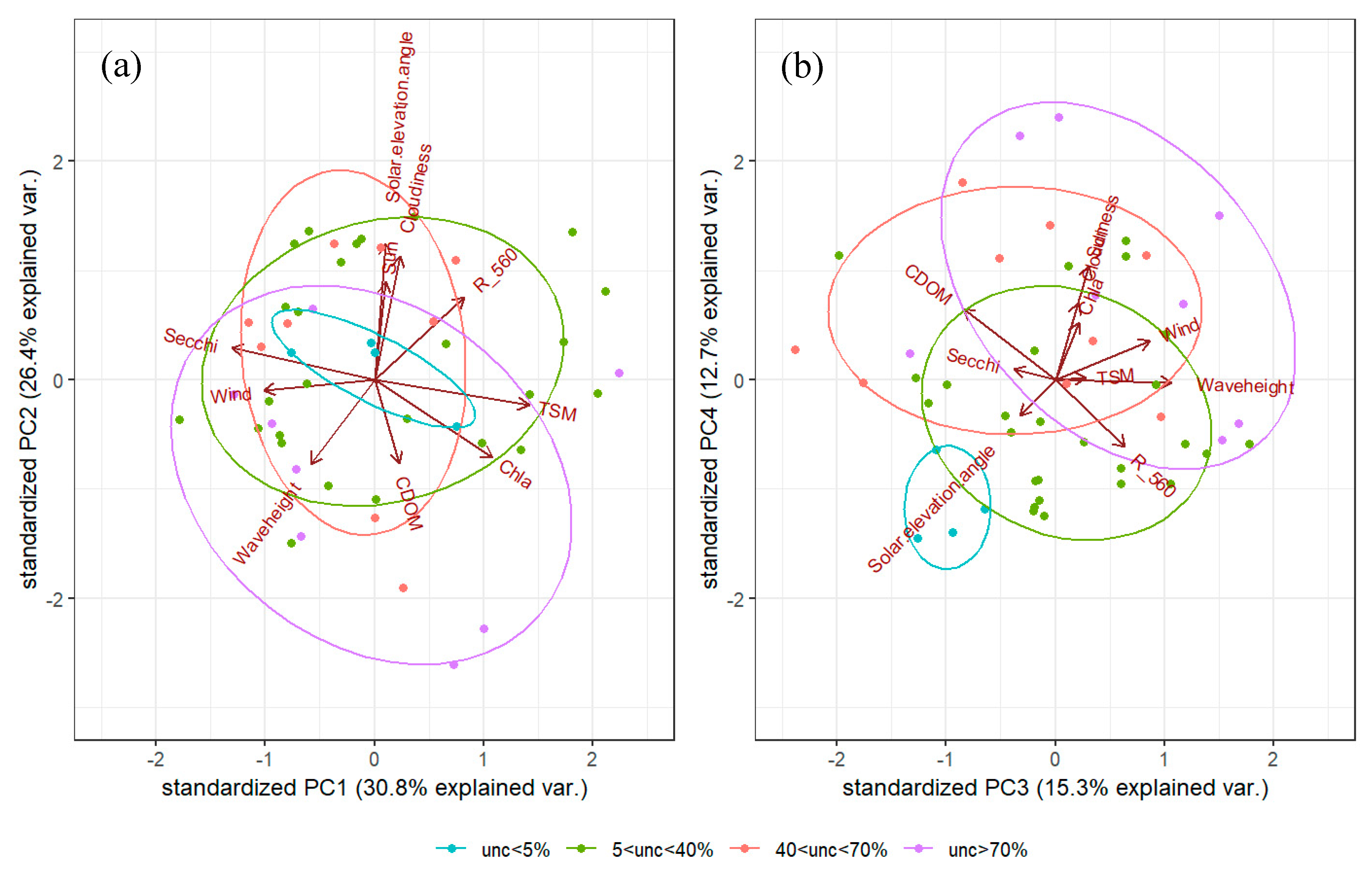
Figure 1 shows the in situ measured water-leaving reflectance processed to OLCIs wavelengths (a), corresponding uncertainty estimates (b) and the relationship between the R_rs and uncertainty (c) on selected wavelengths.

The uncertainties are highest in short visible bands from 400 nm and decreasing toward green wavelengths (560 nm). For bands starting from 753.75 nm, the uncertainties are increasing toward longer wavelengths.

Table A1. Cumulative frequency of measurements with categorized uncertainty estimate, u(R_rs), for every OLCI band. The lowest row shows the median uncertainty for every band. Total 59 in situ measurements.

u(Rrs)	400	412.5	442.5	490	510	560	620	665	673.75	681.25	708.75	753.75	778.75	865	885
<5	6	7	9	21	26	31	31	29	28	28	28	11	10	4	4
<10	12	12	21	32	33	37	36	35	35	35	35	24	23	11	11
<20	22	26	33	35	45	51	50	46	44	45	43	32	32	25	22
<50	37	40	48	53	56	58	57	57	57	57	56	42	41	35	33
50–100	59	59	59	59	59	59	59	59	59	59	59	59	59	59	59
Median	31.9	26.4	17.5	8.7	6.8	3.9	4.2	5.2	6	5.9	5.7	16.2	15.7	27.4	31.7

shows that the median uncertainty is less than 10% for bands 490–708.75 with the lowest median uncertainty of 3.9% for the 560 nm band. For bands 510–708.75, 50% of the measurements were obtained with <5% uncertainty, whereas for bands 400–442.5 and 753.75–885, less than 15% of the measurements were obtained with <5% uncertainty (Table A1).

Figure 1c shows elevated uncertainty for some measurements in case of a weaker signal from the water; however, there is still a cluster of measurements with lower uncertainties independent from the signal strength.

To show the contribution of various components to the full uncertainty budget, data from two stations with similar optical water quality but having different environmental conditions (wind speed, cloudiness) were analyzed.

The left panel in Figure 2 shows spectra measured at one station in challenging conditions (upper panel): wind speed 2 m·s⁻¹, overall cloudiness 90%, sun partially covered during the measurements (ID 839 in

Table A2. Overview of match-up dataset. The bio-optical properties, recorded environmental conditions and radiometric data at the 560 nm band, measured in situ and obtained from tested AC processors.

ID	Secchi (m)	TSM (gm3)	Chla (mg m3)	aCDOM (m−1)	Sun *	Solar .elev	Cloud (%)	Wind (m s)	Wave Height	Dist (km)	Unc (%)	In Situ Rrs	Sat_med Rrs	Difference (%) from the AC Median Rrs					Difference (%) from the In Situ Rrs
														Poly	L2	ALT	C2R	insitu	Poly	L2	ALT	C2R
735	0.7	10.8	34.7	2.5	1	51	90	3.4	0.05	4.8	9.3	0.018	0.026	21	−21	NA	NA	32	−16	−78	NA	NA
782	0.75	15.3	36.3	3.8	1	36	30	0	0	1.8	2.5	0.021	0.016	−10	10	18	−17	−27	13	29	35	8
783	0.8	15.3	37.2	3.2	1	43	10	2.5	0.05	0.8	1.6	0.023	−0.013	NA	0	NA	NA	286	NA	154	NA	NA
784	1.4	9.7	15.7	1.7	1	53	5	1.5	0.05	7.8	1.8	0.020	0.012	−65	7	0	NA	−64	0	43	39	NA
785	1.6	6.6	10.3	1.5	1	55	5	3.5	0.1	2.6	1.1	0.014	0.011	−37	23	4	−4	−32	−4	41	27	21
786	1.4	8.6	13.8	1.5	1	53	5	1	0	12.9	1.1	0.018	0.017	−6	5	−3	3	−5	0	10	3	8
787	1.4	6.3	9.2	1.8	1	45	5	3.5	0.15	14.1	2.3	0.021	0.021	−4	5	0	NA	−4	0	9	4	NA
788	1.4	7.1	14.0	1.5	1	37	5	5.5	0.3	6.6	3	0.024	0.020	−3	5	0	0	−23	17	23	19	18
789	1.4	6.3	10.6	1.6	1	29	7	5	0.2	7.0	3	0.022	0.020	−1	0	13	NA	−10	9	9	21	NA
790	1.8	8.8	20.2	1.4	3	37	60	5	0.2	7.3	11.8	0.017	0.016	−11	11	NA	NA	−11	0	20	NA	NA
791	1.6	5.8	19.2	1.5	3	45	60	5	0.2	6.6	11.7	0.015	0.014	−11	11	NA	NA	−6	−4	16	NA	NA
792	1.7	7.7	19.9	1.3	3	51	90	5.5	0.15	14.1	10.3	0.017	0.013	−7	7	NA	NA	−30	18	28	NA	NA
794	1.4	5.8	17.8	4.2	3	47	100	4.5	0.15	2.7	28.6	0.009	−0.010	NA	0	NA	NA	194	NA	206	NA	NA
832	0.45	16.3	31.9	2.5	1	46	30	0	0.15	3.0	5.7	0.032	0.019	−4	4	−5	36	−65	37	42	37	62
833	0.5	24.7	36.1	2.4	1	48	35	0.5	0.05	3.0	5.8	0.030	0.028	−3	−3	9	3	−6	3	3	14	9
834	0.5	16.7	35.5	2.0	1	51	50	0	0.05	4.8	8.3	0.036	0.040	2	−3	15	−2	12	−11	−17	4	−15
835	0.4	20.0	30.1	2.3	1	53	80	0	0.005	0.5	3.8	0.042	0.045	0	−24	NA	24	6	−6	−31	NA	19
838	0.9	12.5	28.2	2.8	3	47	100	3	0	3.0	12.1	0.024	0.019	NA	55	0	0	−28	NA	65	22	22
839	1.35	9.1	15.0	2.3	3	50	90	2	0.05	0.9	10.7	0.017	0.002	NA	0	NA	NA	−905	NA	90	NA	NA
841	0.65	9.7	22.0	4.7	3	50	80	2.5	0.05	0.7	13.6	0.012	−0.024	NA	0	NA	NA	150	NA	300	NA	NA
842	1.7	4.3	9.5	1.6	1	47	80	5.5	0.15	7.4	13.6	0.014	0.014	−3	45	0	0	0	−3	45	0	0
894	1.8	7.7	28.5	1.8	2	36	60	5	0.4	7.8	43.7	0.014	0.018	−5	7	5	−13	23	−36	−21	−23	−47
898	1.1	6.8	20.5	1.2	1	31	25	5	0.4	13.6	13.7	0.019	0.009	2	−2	9	−4	−107	52	51	56	50
899	0.9	10.5	25.5	1.6	1	35	10	6	0.4	12.9	10.5	0.022	0.019	−7	−2	2	4	−14	6	10	14	16
900	0.8	12.5	24.8	1.9	1	33	10	4	0.4	2.4	11.1	0.022	0.018	−16	2	−2	25	−24	6	20	18	40
901	0.7	12.0	34.3	4.8	1	29	5	3	0.4	7.3	20.9	0.013	0.015	10	32	−10	−12	14	−5	21	−28	−31
903	0.6	17.5	55.3	3.4	1	20	10	2	0.3	3.1	78.3	0.005	0.022	−3	6	3	−19	79	−402	−355	−369	−478
1981	0.7	16.0	29.1	3.5	3	35	60	1	0.01	0.6	21	0.005	−0.057	NA	0	NA	NA	109	NA	1224	NA	NA
1982	0.7	17.5	48.5	3.4	3	41	70	2	0.1	3.1	5	0.019	0.022	9	−4	4	−46	14	−6	−21	−12	−71
1983	1.2	7.7	17.5	1.8	1	44	65	3	0.1	0.9	15.6	0.015	−0.003	NA	0	NA	NA	646	NA	118	NA	NA
1985	1.1	8.4	19.6	1.9	1	46	60	2	0.1	7.8	2.2	0.016	0.017	5	8	−5	−5	6	−2	2	−12	−13
1986	1.3	6.0	25.4	1.7	1	46	30	2	0.1	12.9	2.3	0.014	0.014	3	13	−3	−3	1	1	11	−4	−4
1987	1.4	7.3	24.6	1.7	3	40	25	4	0.2	13.8	3.9	0.014	0.015	−5	9	−4	4	6	−12	3	−11	−2
2205	0.9	12.7	16.7	NA	4	29	60	2	0.01	0.9	3.7	0.027	0.017	−26	35	NA	0	−57	20	58	NA	36
2207	0.9	14.6	27.4	NA	4	42	50	2	0.15	0.5	1.8	0.025	0.015	−60	0	13	NA	−63	2	39	47	NA
2208	0.9	14.5	26.1	NA	4	46	40	1	0.1	1.6	1.5	0.027	0.023	−4	7	4	−9	−15	10	19	16	5
2209	0.9	10.8	20.3	NA	4	50	80	0.5	0.05	0.3	1.2	0.027	0.025	7	−7	21	−9	−8	14	1	27	−1
2210	0.9	8.7	13.9	NA	4	52	100	1	0.1	3.6	1.2	0.025	0.023	−5	11	5	−6	−8	3	18	12	3
2211	0.9	9.4	27.0	NA	4	51	80	3	0.2	1.8	1.3	0.010	0.007	−35	37	6	−6	−41	4	55	34	24
2212	1	7.4	9.6	NA	4	50	80	4	0.2	3.2	1.8	0.020	0.020	−6	16	NA	0	−1	−5	17	NA	1
2228	2	1.5	6.8	3.1	1	50	10	5	0.3	2.7	1.8	0.006	0.003	−105	105	NA	NA	−139	14	102	NA	NA
2230	1.6	4.0	9.0	3.2	1	43	40	3	0.1	13.9	27.2	0.003	0.003	24	−24	NA	NA	3	22	−27	NA	NA
2232	2.3	3.5	8.5	2.1	1	36	70	1	0	8.5	11.1	0.006	0.006	2	−2	NA	NA	1	1	−3	NA	NA
2284	1.2	5.7	15.1	5.7	1	43	0	4	0.15	3.2	3.2	0.004	−0.003	NA	0	NA	NA	248	NA	168	NA	NA
2285	1.2	5.1	13.1	5.8	1	46	0	4	0.2	1.4	3.3	0.004	0.001	−243	243	NA	NA	−479	41	125	NA	NA
2286	1.8	6.0	11.1	4.1	1	48	3	4	0.3	7.3	4	0.004	0.001	−102	102	NA	NA	−204	34	101	NA	NA
2288	1.4	3.8	8.5	4.0	1	49	20	4	0.2	13.0	2.5	0.004	0.003	−18	18	NA	NA	−45	19	44	NA	NA
2578	0.7	22.3	34.7	3.2	2	37	80	4.5	0.4	1.4	2.9	0.022	0.023	1	0	−23	NA	3	−2	−3	−26	NA
2579	0.5	23.0	49.8	3.2	2	43	80	4	0.2	3.2	6	0.023	0.020	−11	33	−25	11	−17	5	43	−6	24

* Clear—1; fully covered—2; partially covered—3; through thin cloud—4.

) and in good conditions (lower panel): wind speed 1 m·s⁻¹, overall cloudiness 5%, no clouds in front of the sun (ID 786 in Table A2). For both stations, the median hyperspectral spectra and the ones calculated on OLCIs wavelengths (blue) have similar shape and magnitude, although they greatly differ based on the uncertainty estimates (gray line). The uncertainty budget (on the right panel in Figure 2) shows the main contribution comes from environmental conditions for the upper panel due to the high standard deviation in the station spectra caused by changing and challenging environmental conditions during the measurements. The good measurement conditions resulted in a lower standard deviation and there is no domination of one certain component to the full uncertainty budget (Figure 2, lower panel).

3.2. PCA

To study the factors associated with different levels of uncertainty in the R_rs data (Figure 2a,b), a PCA was applied on the full in situ dataset. Ten input parameters were used for the PCA: TSM, Chl a, a_CDOM(442), Secchi depth, R_rs(560), solar elevation angle, overall sky cloudiness, wind speed, wave height, sun conditions. This resulted in 10 principal components and the contribution from each parameter is shown in

Table 2. Principal Component Analysis (PCA) components (PC1–PC10) and contribution by measured parameters. Parameters with highest contribution to first four principal components are marked in bold. The lowest row shows the cumulative proportion (%) of each component to the total variation.

Parameters	PC1	PC2	PC3	PC4	PC5	PC6	PC7	PC8	PC9	PC10
TSM (g·m−3)	0.53	−0.09	0.15	0.01	0.07	0.01	0.19	0.12	−0.55	0.57
Chl a (mg·m−3)	0.41	−0.29	0.11	0.31	0.27	−0.22	0.33	0.32	0.13	−0.54
aCDOM(442) (m−1)	0.09	−0.31	−0.45	0.38	−0.59	−0.03	−0.25	−0.02	−0.33	−0.18
Secchi (m)	−0.49	0.12	−0.20	0.06	0.40	0.11	0.14	0.23	−0.64	−0.22
Rrs(560) (sr−1)	0.31	0.31	0.34	−0.36	−0.22	0.32	−0.32	0.16	−0.25	−0.47
Solar elevation angle (°)	0.04	0.51	−0.17	-0.19	−0.39	−0.46	0.55	−0.04	−0.08	−0.10
Overall sky cloudiness (%)	0.09	0.46	0.11	0.41	0.22	−0.52	−0.52	−0.01	−0.06	0.06
Wind speed (m·s−1)	−0.38	−0.04	0.46	0.21	−0.39	−0.05	0.05	0.63	0.07	0.19
Wave height (m)	−0.22	−0.31	0.57	−0.01	−0.08	−0.29	0.07	−0.56	−0.30	−0.17
Sun conditions *	0.04	0.37	0.16	0.61	−0.08	0.52	0.29	−0.31	0.04	−0.02
Cumulative Proportion	31	57	73	85	91	94	97	98	99	100

* Clear—1; fully covered—2; partially covered—3; through thin cloud—4.

.

Based on the calculated uncertainty budget on the 442 nm band, four categories based on the level of uncertainty were derived: (1) u(442) < 5%, (2) 5% ≤ u(442) < 40%, (3) 40% ≤ u(442) < 70%, (4) u(442) > 70%. This was used as an additional layer of information for each point in interpreting the PCA results.

The first principal component (PC1) described 30.8% of variance in the dataset and had the highest contribution from TSM, Chl a and Secchi depth (Table 2, Figure 3). Therefore, PC1, the group explaining the highest variation in the in situ data, can be associated with the optical properties of the water. Figure 3 shows how each in situ measurement is positioned in terms of principal components and associated level of uncertainty estimated at the 442 nm band. There is no association between the level of the uncertainty and the variables contributing most to PC1 (Figure 3). PC2, describing 26.4% of the variance, can be associated mainly with changes in the solar elevation angle and overall sky cloudiness (Table 2). Based on the PCA results, neither PC2 can be used to differentiate points with different levels of measurement uncertainty.

Based on PC3 and PC4, different clusters were formed in terms of low (<5% uncertainty at the 442 nm band) and high (>70% uncertainty at the 442 nm band) measurement uncertainty (Figure 3). Both PC3 and PC4 are determined by environmental conditions. The main contribution to PC3 comes from wave height and wind speed, to PC4 from sun conditions (if there are clouds in front of the sun or not) and overall sky cloudiness (Table 2). Based on the PC3 and PC4, measurements with a lower level of uncertainty are associated with lower wave height and wind speed (PC3) and also good illumination conditions (clear sky and no clouds in front of the sun) (PC4).

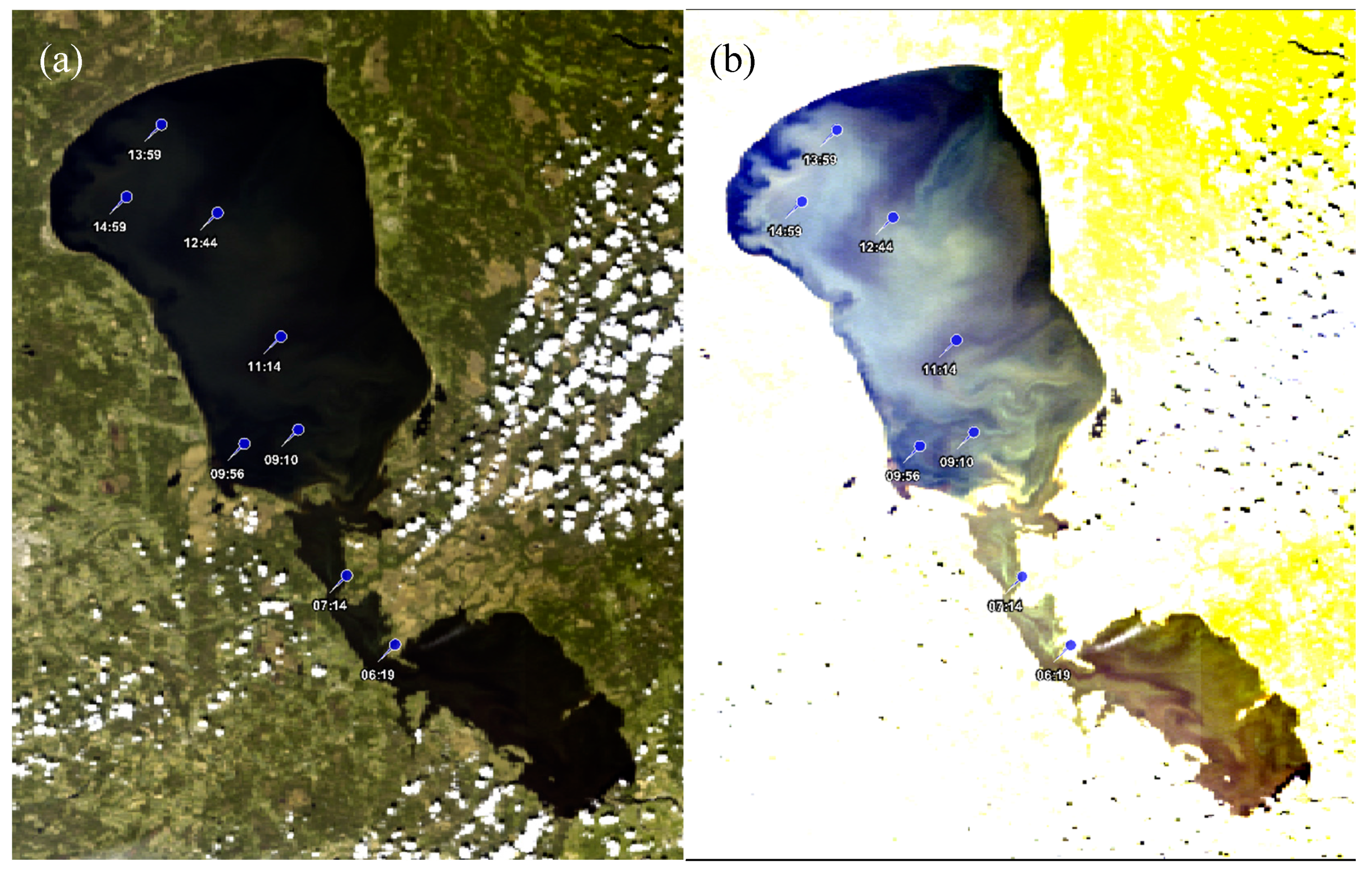
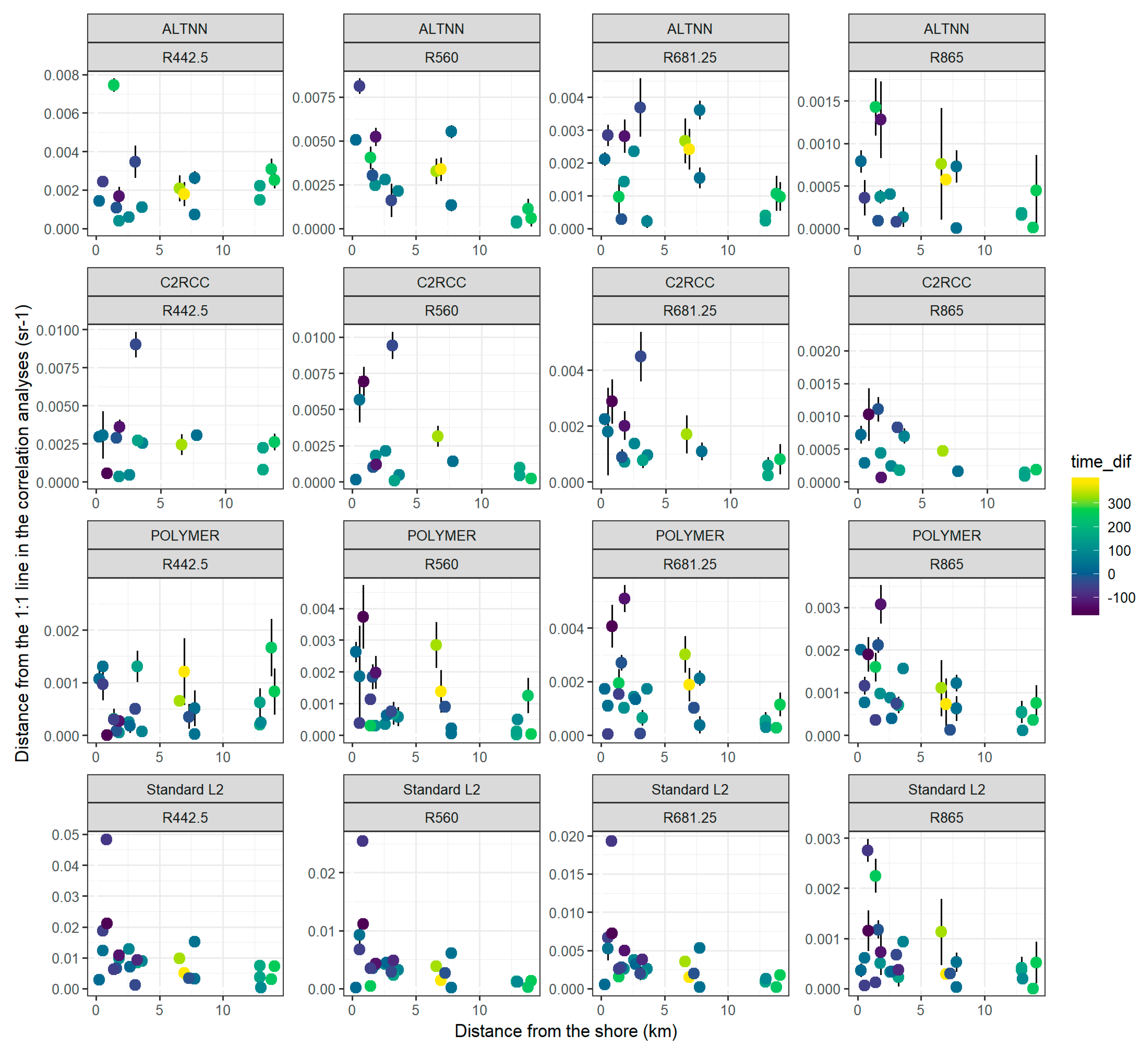
3.3. Spatial and Temporal Effects on Combining Satellite and In Situ Data

The S3A OLCI image (Figure 4) coupled with in situ sampling dataset from 14 June 2016 was analyzed for the performance of various AC processors in comparison with in situ data in terms of changing temporal and spatial conditions.

The reference measurements, derived R_rs from AC processors and environmental conditions for each station, are shown in Figure 5. Each measurement was performed in conditions where no clouds were in front of the sun (Figure A1). The overall sky cloudiness was higher in the first two stations (from 30% to 10%, respectively) but stayed constant at 5% for the following stations (Figure A1). The clouds were Cirrus and Cirrostratus for the three first stations, and later Cumulus and Cirrostratus. Wind speed changed from 0 to 5.5 m/s and wave height from 0 to 0.3 m, both increasing toward the evening (except at station #5, at 11:14 UTC, Figure A1). The in situ measured R_rs(λ) with associated uncertainties compared to quality-controlled AC retrievals (Figure 5) show that, although the image was cloud-free (Figure 4), the number of retrievals varies station-by-station. The lower two panels (Figure 5) shows the ratio of the AC processor-derived R_rs(λ) to the in situ measured R_rs(λ) with respective uncertainty. The uncertainties are higher in the first and last three stations, while stations #2 to #5 have very low uncertainties as the measurements have been performed in conditions with low wave height and wind speed in combination with a solar elevation angle above 40 degrees. The optical properties of water are similar in the first two stations (Figure A1), where the main changes are in the overall sky cloudiness (decrease from 30% to 10%), solar elevation angle (from 36 to 43 degrees) and a slight increase in wind speed (from 0 to 2.5 m/s) and wave height (from 0 to 0.05 m).

In the first two stations, the Chl a, TSM and a_CDOM absorption are the highest and decrease in the following stations, where they stay fairly the same (Figure A1).

The best performance from each AC processor is in the case of station #5 measured at 11:14 UTC where all processor-derived R_rs pass the quality control by flags. This station is about 13 km away from the coast. The most complex conditions were for station #2 of the day (at 7:14 UTC), where measurements were performed in a very narrow part of the lake (Figure 4), just 0.8 km from the nearest coast.

Figure 5a shows the changes in the R_rs uncertainty during one measurement campaign. Uncertainty was higher during early morning and evening measurements which can be linked with the sun elevation angle (Figure A1) and also with the wind speed in the evening measurements (3.5–5 m·s⁻¹). During the midday station, in good measurement conditions (Figure A1), the uncertainties stayed low in the whole spectrum, e.g., station #4, where uncertainty was 1.1–1.5% for bands 490–708.75, and between 2% and 6.5% for shorter and longer wavelengths. In contrast, in the second to last station, #7, the uncertainty was 3–5.9% for bands 490–708.75, and between 12.1% and 33% for shorter and longer wavelengths, which can be explained by changes in the environmental conditions, e.g., lower sun elevation angle (36.7 degrees) and higher wind speed (5.5 m·s⁻¹).

Although the uncertainties for the first three OCLI bands (up to 442.5 nm) are higher, the AC processor-derived R_rs is only derived in the limits of uncertainty by POLYMER AC in few cases; all other AC results tend to under- or overestimate. While the standard AC strongly underestimates bands up to 560 nm, its accuracy is comparable with other processors for longer wavelengths. For bands 665, 673.75 and 681.25, AC-derived R_rs is slightly (about 20–30%) underestimated. While POLYMER tends to show the most accurate spectra, it has the highest inaccuracies at the 865 nm band, where all other AC processors perform better.

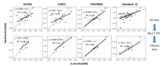
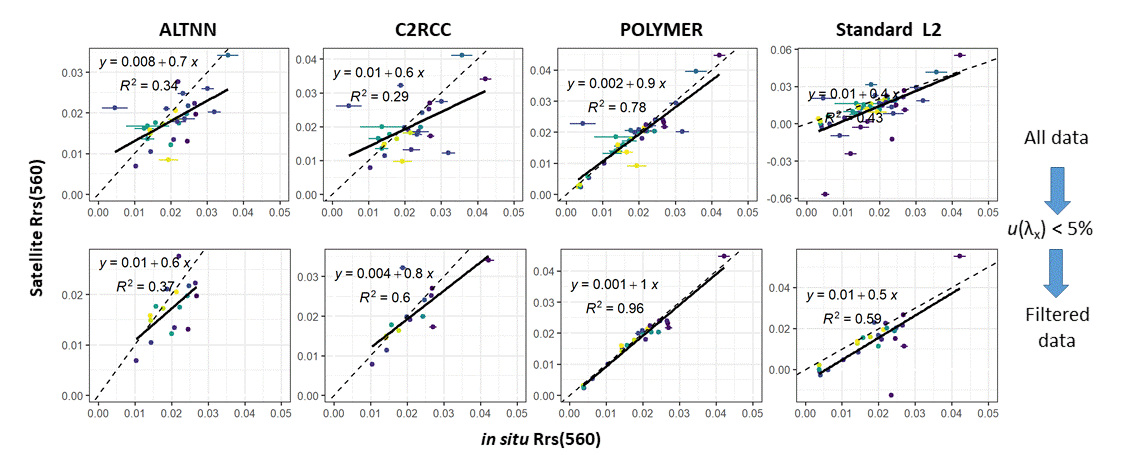
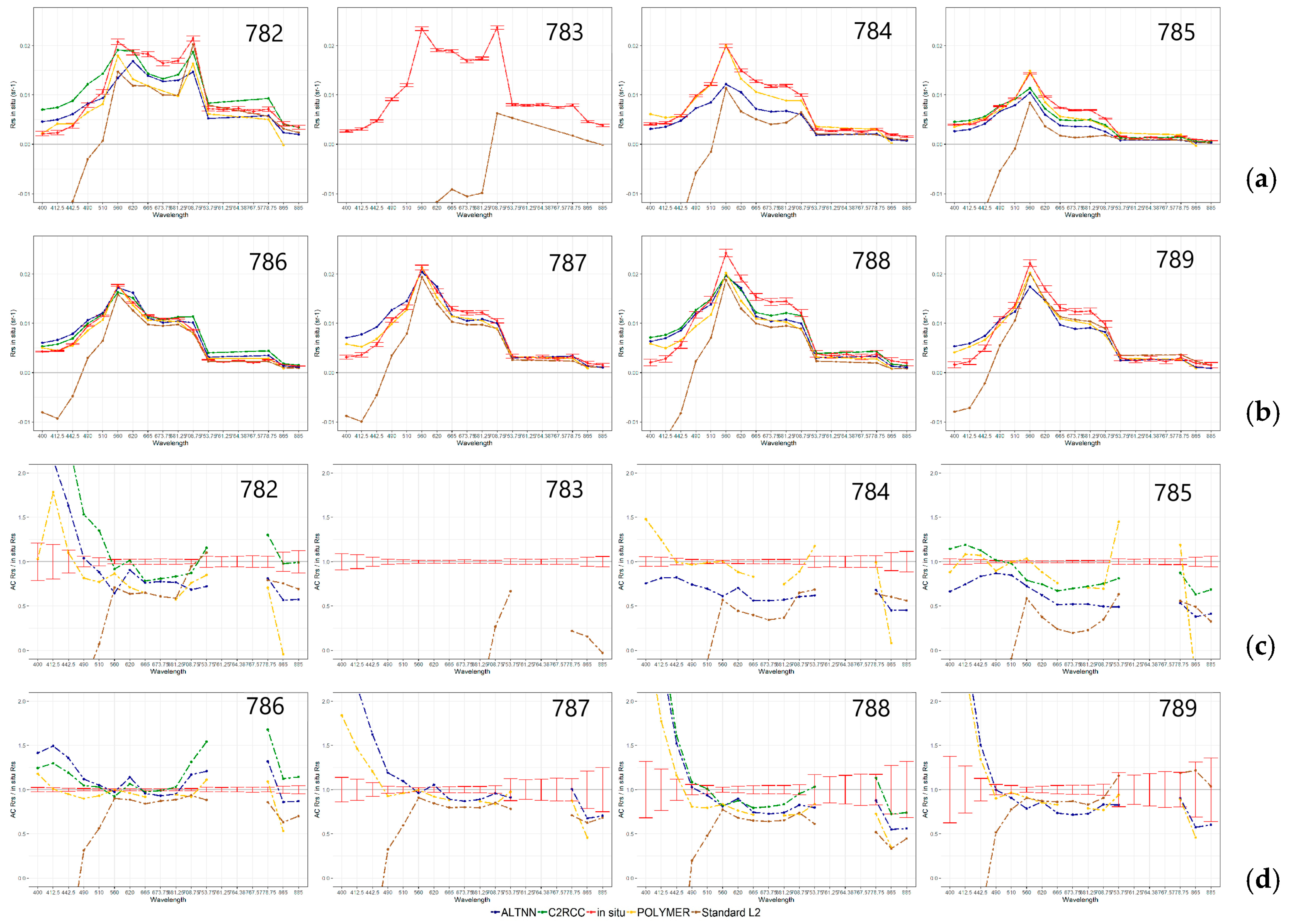
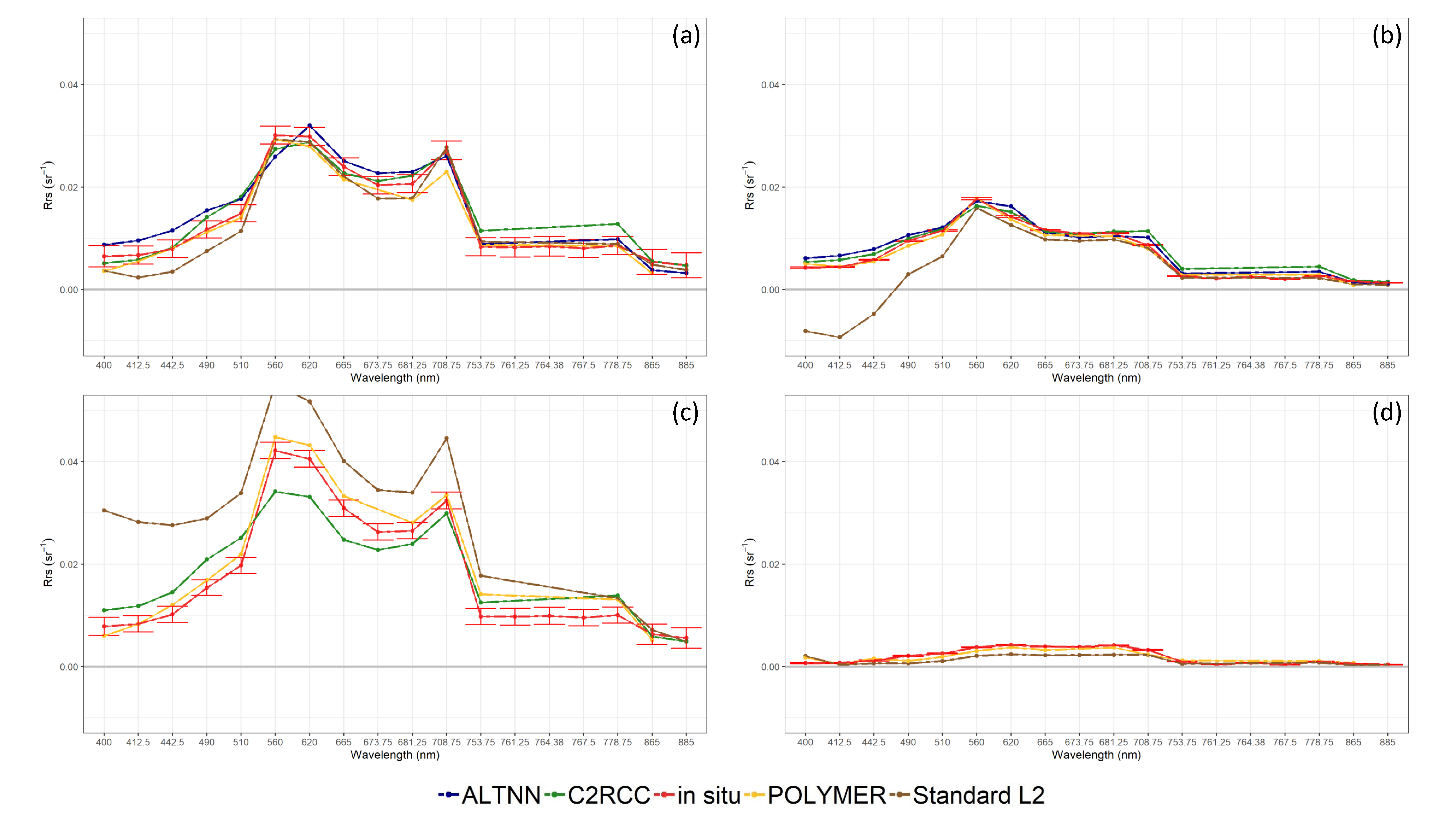
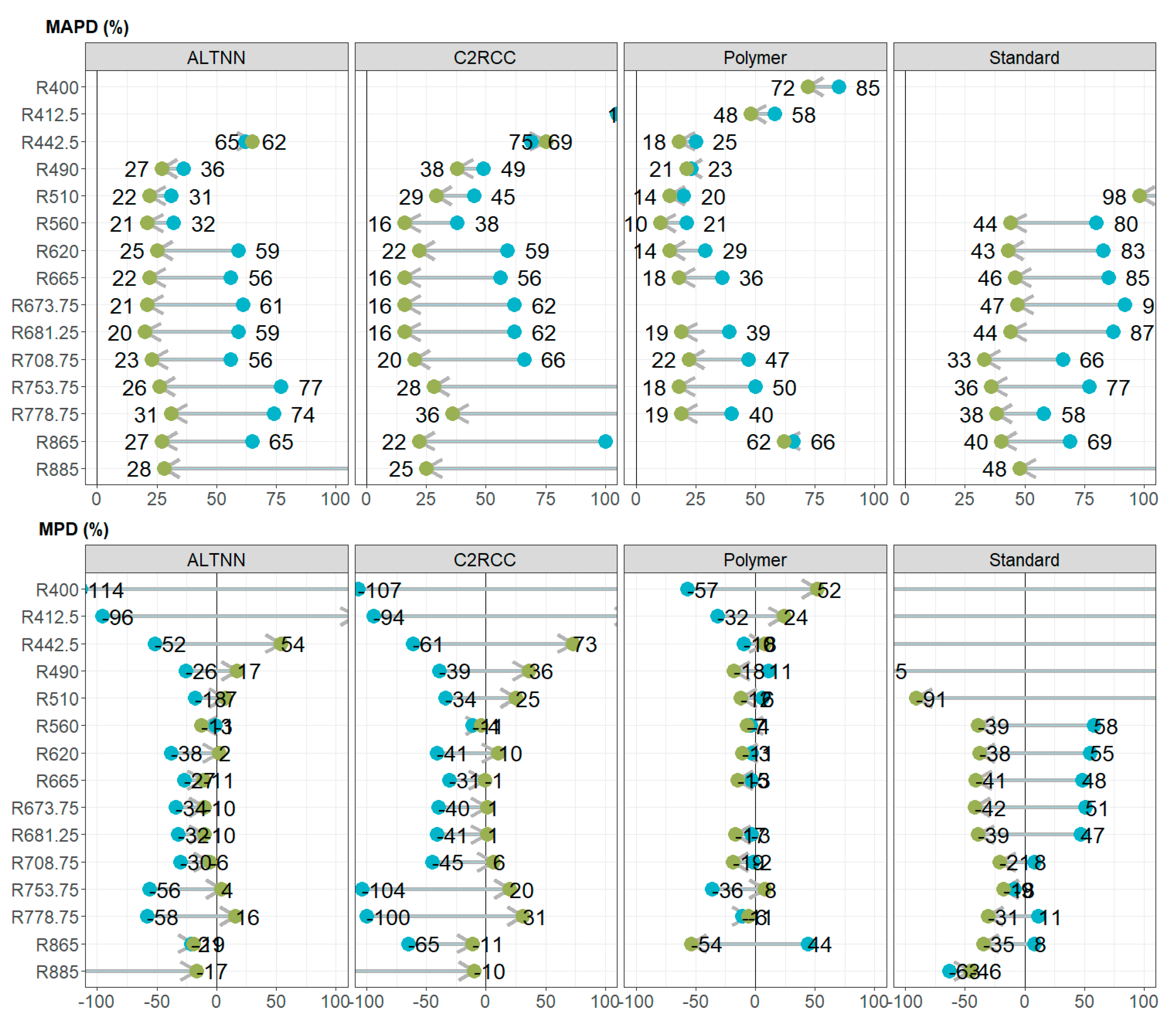
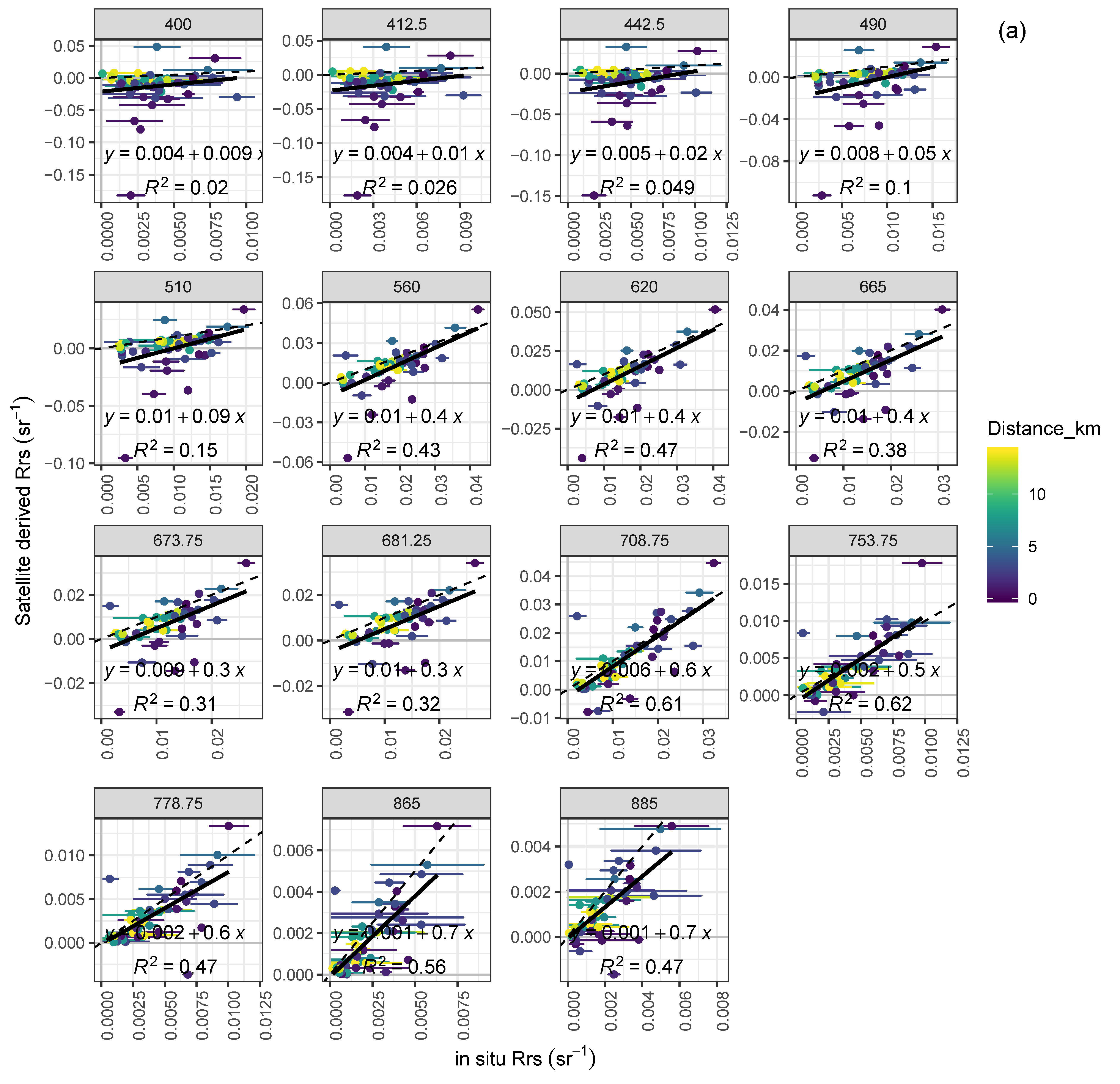
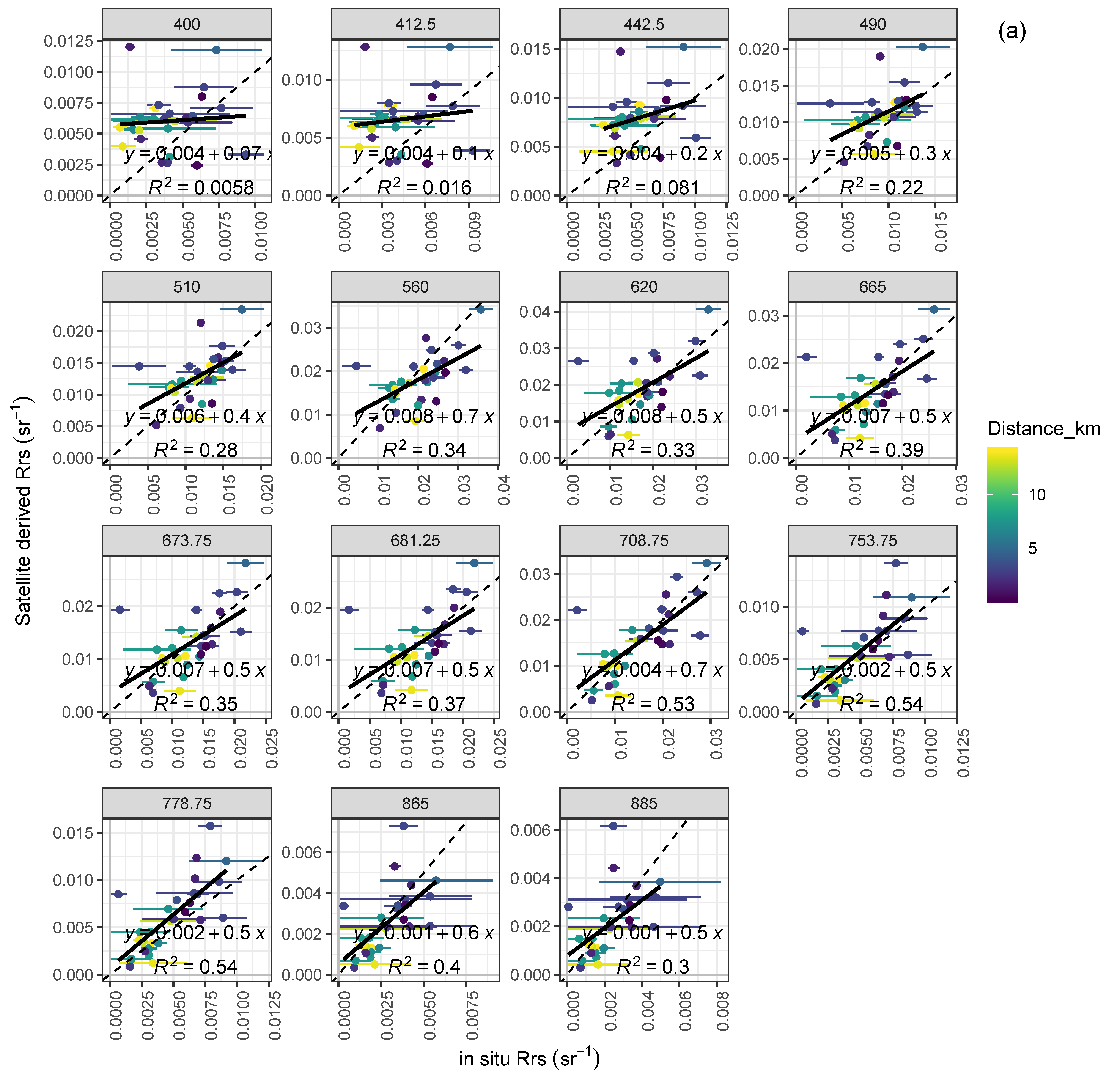
3.4. Validation of AC Processors on All Match-Ups

Visual observation of spectra from all match-up stations showed that in productive waters (Chl a > 20 mg·m⁻³), the products of C2RCC and ALTNN (Figure 6a) tend to give peak reflectance at 620 nm instead of 560 nm as measured in situ. C2RCC and ALTNN products are often flagged out over absorbing waters (a_CDOM > 1.5 m⁻¹) with Chl a level < 20 mg·m⁻³ (Figure 6d, ID 2228-2288 in Table A2) regardless of the distance from the shore. It was also noted that the agreement between the processors increases further away from the shore (Figure 6b), except the bands up to 510 nm in case of standard product. In the vicinity of land (Figure 6c), the discrepancies between the various AC processors become higher, although the POLYMER tends to be least affected by the adjacency effect.

Table A2 shows the overview of bio-optical properties, environmental variables and adjacency to land for each match-up point with a reference to R_rs at 560 nm, measured in situ or derived by AC processors. Combining the results from regression analyses (Figure A2, Figure A3, Figure A4 and Figure A5) and Table A2, good conditions for satellite retrievals can be associated with high distance from the land (>7 km,, e.g., ID 786, 787, 842, 1985 and 1986 from Table A2) in combination with good illumination conditions (clear in front of sun, wind speed 0.5 to 5.5 m·s⁻¹, wave height < 0.15 m). The uncertainties at 560 nm stayed under 14%. In these cases, the difference between the processors was usually < 10% and deviation from the in situ < 15% (Table A2). The highest errors between in situ and satellite-derived R_rs (ID 903, 901 in Table A2) can be associated with low solar elevation angle (<30 degrees) in combination with high Chl a (>34 mg·m⁻³) which results in high uncertainty for the in situ measurements (78.3% and 20.9% at 560 nm, respectively). Additionally, measurements performed with high wind speed (5 m·s⁻¹) in combination with high wave height (0.4 m) are associated with higher uncertainties and the errors are high between the AC processor retrievals and situ data (20% to 50%) but low between the processors (2–13%, ID 894, 898 in Table A2).

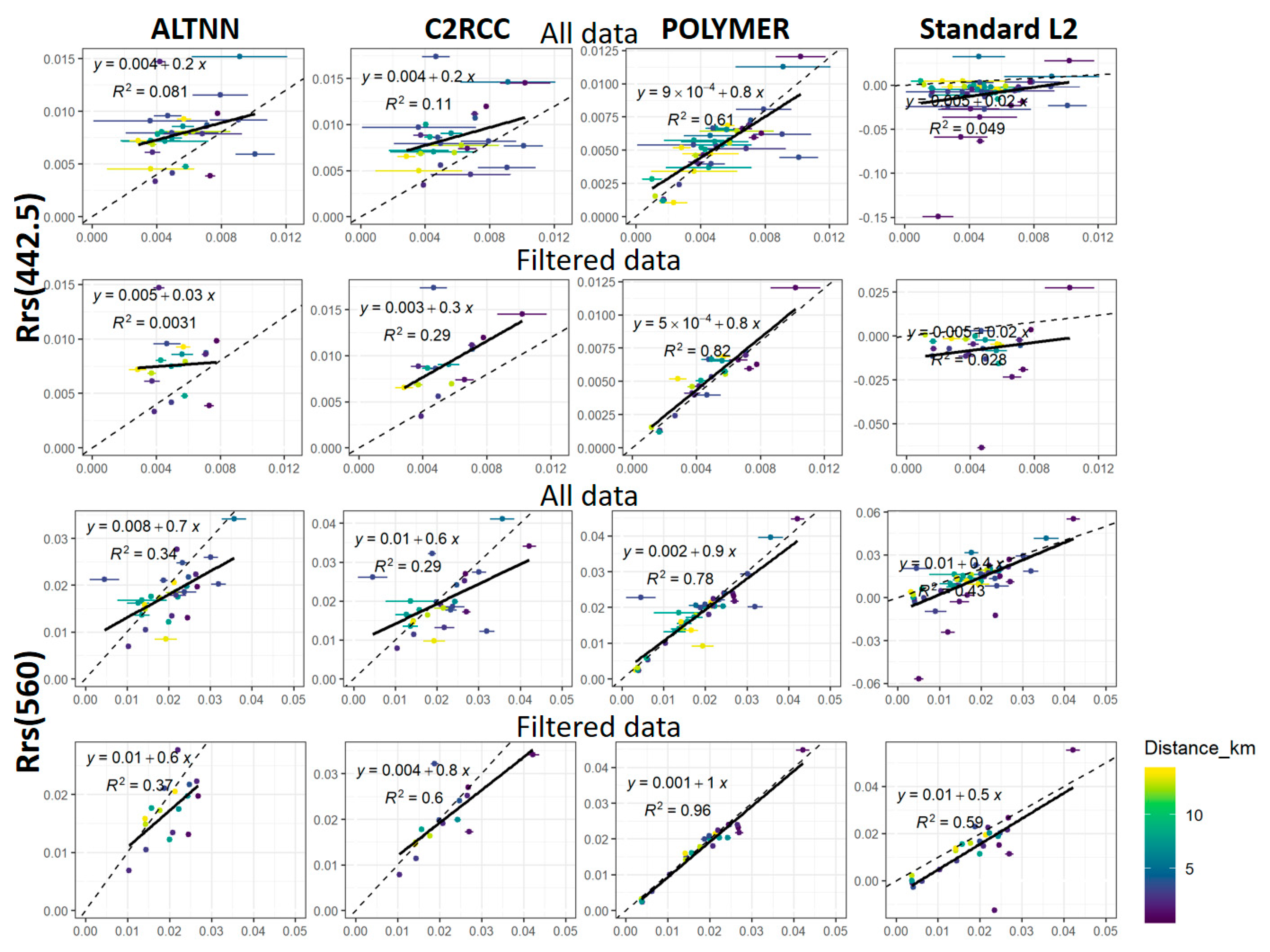
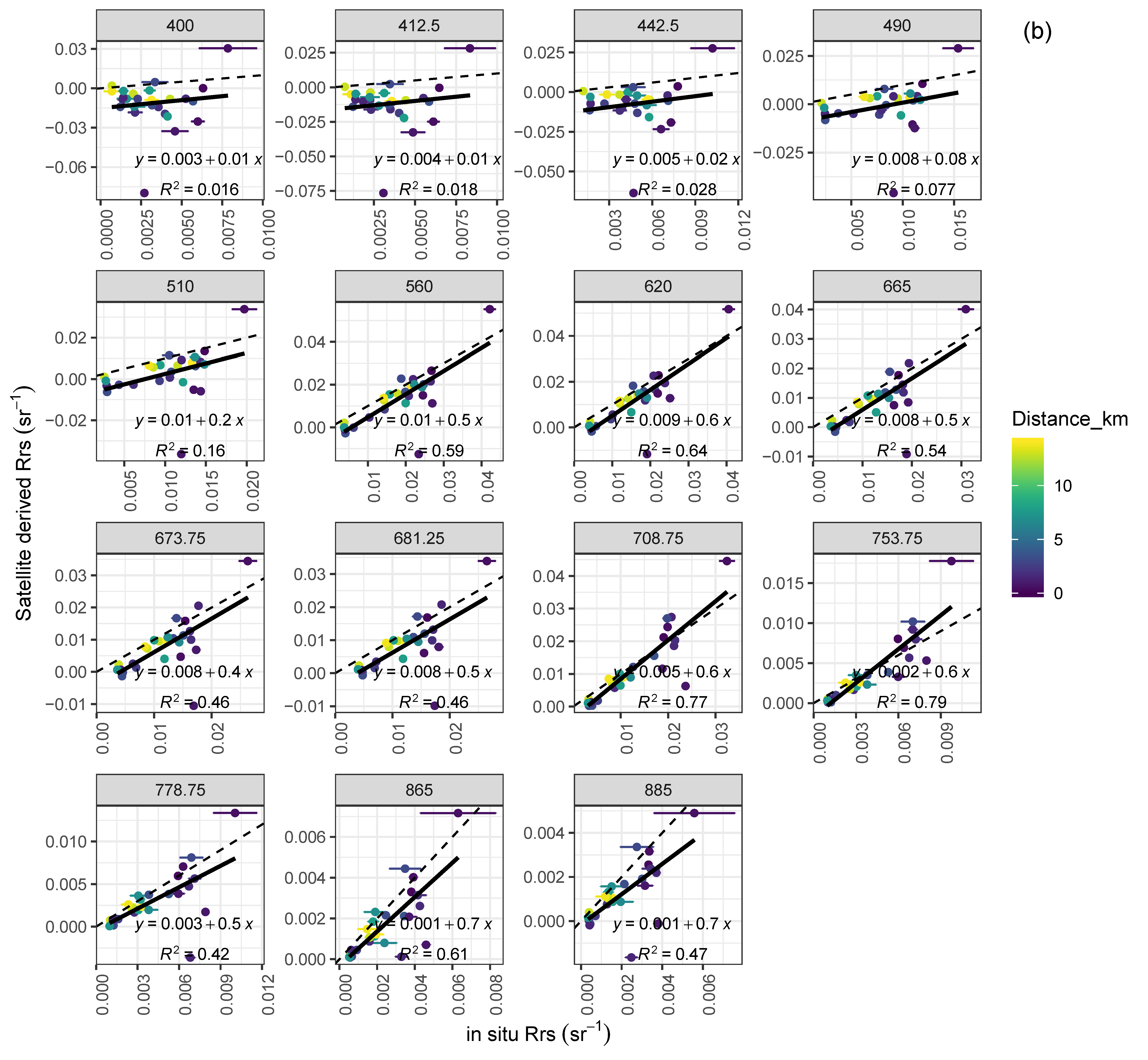
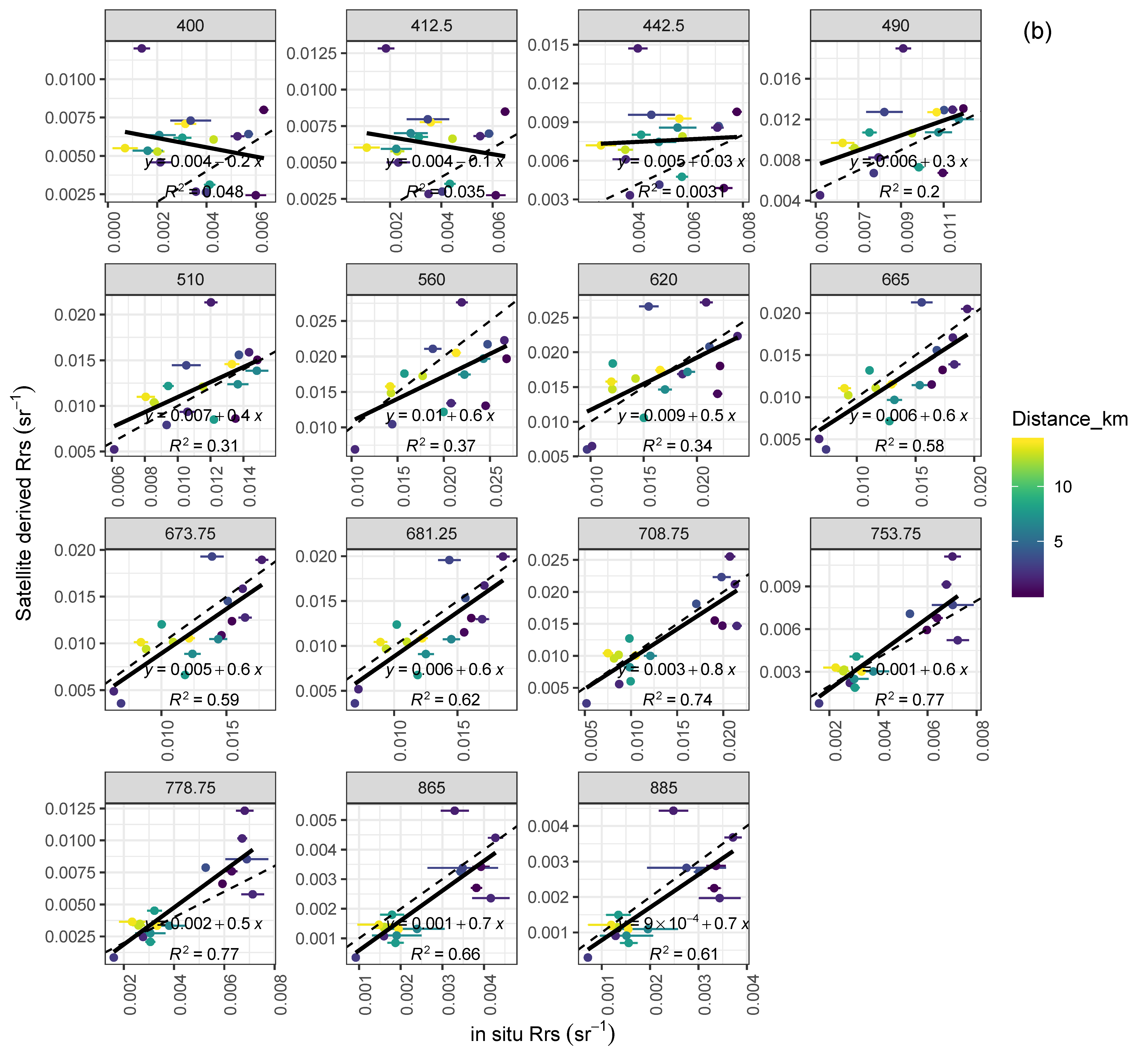
3.5. Filtering the In Situ Data Based on the Uncertainty

The difference between the in situ measured R_rs and AC derived is the highest for the 400 and 412.5 nm bands in the case of each processor (Figure 7, Figure A2, Figure A3 and Figure A4 and Figure A5a). Based on the statistics, the POLYMER-derived R_rs is the most accurate for all bands, except at 865 nm. POLYMER-AC-derived R_rs values are well aligned around at in 1:1 line (Figure A2) with a relatively smaller bias compared to other processors.

Bands up to 510 nm are overestimated by ALTNN and C2RCC (MPD 114% and 107%, respectively, at 400 nm), slightly overestimated by POLYMER (MPD 57%) and strongly underestimated by standard products (MPD −463%). Improved accuracy is obtained for longer wavelengths by all processors. For POLYMER, ALTNN and C2RCC, the band at 560 nm is derived with the highest accuracy, e.g., MAPD 21% (POLYMER), 32% (ALTNN), 28% (C2RCC). In general, for all AC processors, the derived R_rs for bands from 753 nm onwards show higher scatter compared to green bands, although the majority of the estimates are in the limits of the associated in situ measurement uncertainty (Figure 7, and more in detail for each processor in Figure A2, Figure A3, Figure A4 and Figure A5).

As the median uncertainty for the in situ R_rs varies greatly on different wavelengths (Appendix A, Table A1), the filtering of data was made based on the up to 5% uncertainty criteria at least in one band. This eliminated the in situ data measured in not optimal environmental or measurement conditions and improved the accuracy of the AC processor retrievals (Figure 7 and Figure 8 and for each processor separately; Figure A2, Figure A3, Figure A4 and Figure A5). This decrease in match-ups was about 55% for each processor: POLYMER (41 → 24), C2RCC (27 → 15), ALTNN (29 → 17), Standard L2 (49 → 26).

To estimate the reason for outliers in the correlation plots (Figure A2, Figure A3 and Figure A4 and Figure A5b), the distance from the 1:1 line was measured for every point and analyzed against different variables. The outliers were most evident in the adjacency to land in the first five kilometers, and the errors between the AC-derived and in situ measured R_rs decrease with increasing distance from the shore (Figure 9). It is especially pronounced in the standard OLCIs R_rs products, then C2RCC and ALTNN. In the case of POLYMER, the adjacency has the lowest impact on the quality of the retrievals compared to other processors. As the match-up dataset contains data pairs with variable time difference between the in situ measurements and satellite overpass, Figure 9 shows that over these inland and coastal waters, the time difference between −3 h up to +6 h (in situ minus satellite overpass) can be associated with outliers only in few cases.

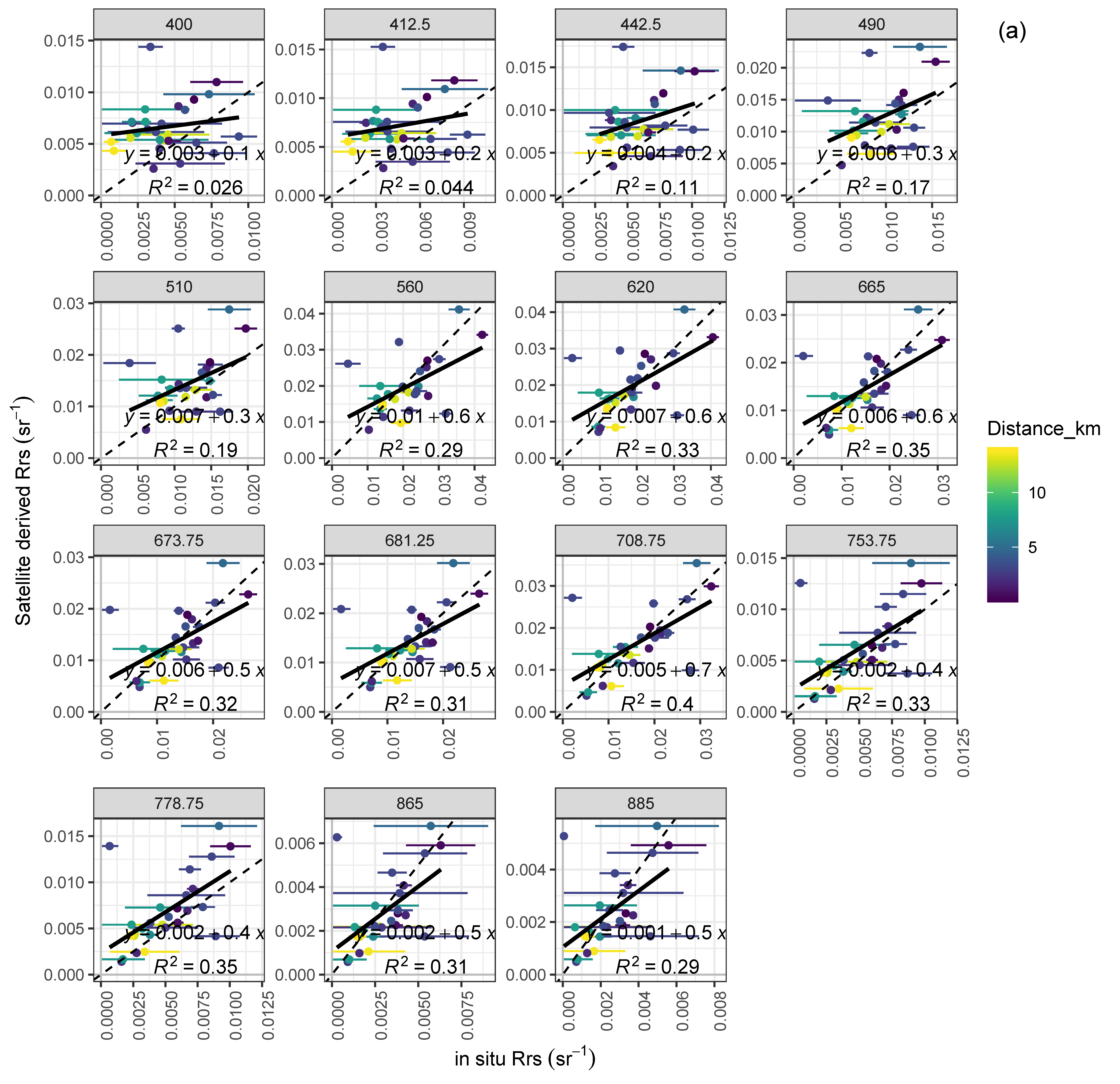
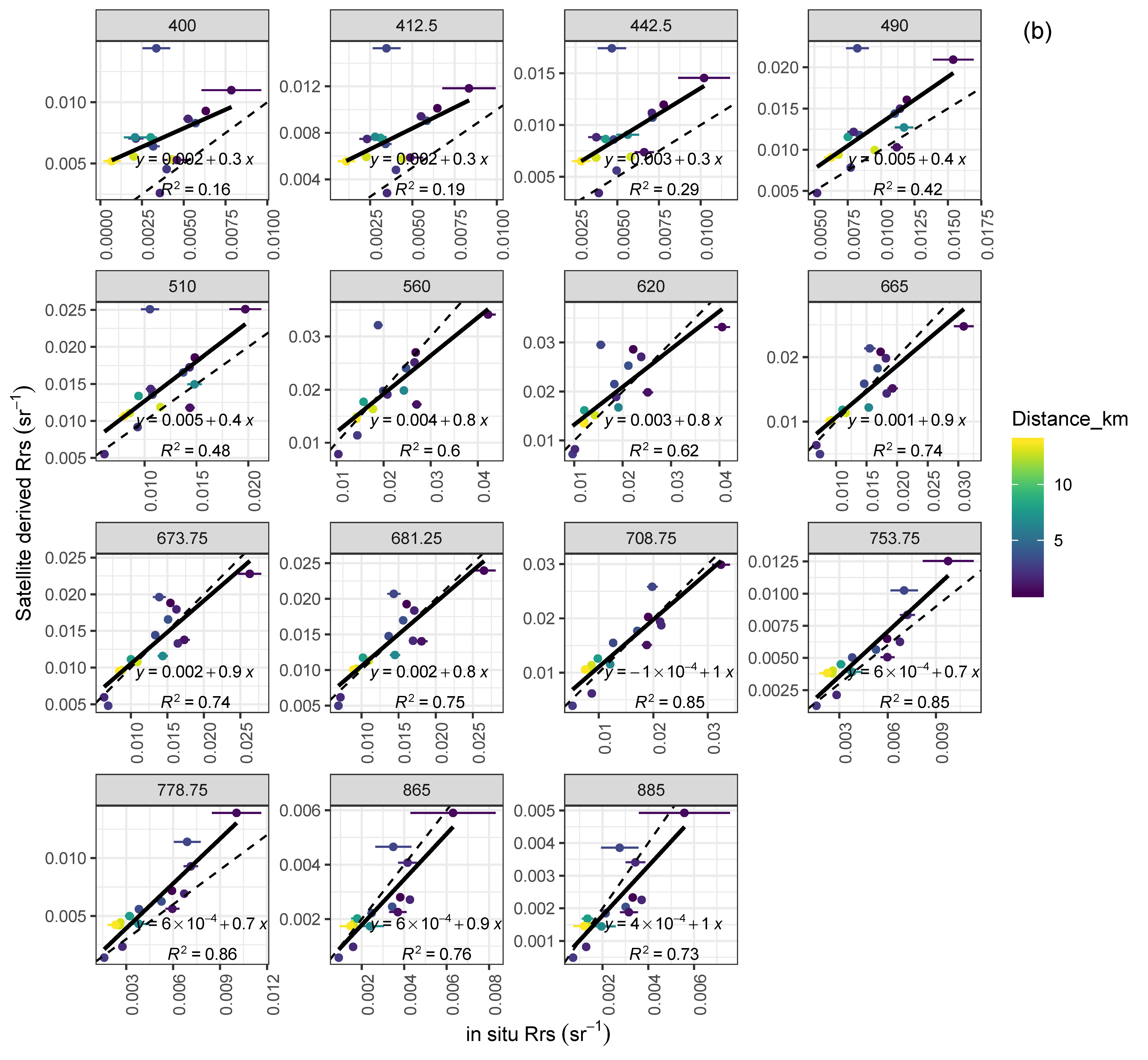
3.6. Comparability between AC Processors

To exclude the conclusions on AC performances due to the different number of match-up points and processor-based flagging, the statistics were calculated only for these stations when all four processors derived quality control retrievals (

Table 3. Statistics on match-up data for tested AC processors only for 22 match-up points when each AC processor (Alternative Neural Net—ALTNN, Case 2 Regional CoastColor Processor—C2RCC) resulted in quality-controlled retrieval.

	MAPD (%)				MPD (%)
Name	Polymer	Standard	ALTNN	C2RCC	Polymer	Standard	ALTNN	C2RCC
400	50	353	109	136	25	−276	97	120
412.5	43	336	93	116	22	−312	83	103
442.5	22	194	56	74	6	−192	50	64
490	22	82	35	52	−5	−82	28	40
510	24	56	31	48	−2	−51	21	36
560	29	38	35	42	14	−2	7	16
620	40	49	71	69	16	4	52	51
665	51	62	67	64	20	12	41	39
673.75	NA	68	73	72	NA	14	48	49
681.25	56	66	70	72	21	16	46	50
708.75	64	73	68	78	24	40	42	55
753.75	75	97	93	138	55	58	72	122
778.75	56	71	88	125	24	25	71	114
865	70	90	76	119	−50	32	32	81
885	NA	268	241	421	NA	214	198	386

). These eliminated all the match-up stations representing a_CDOM-rich waters because none of the C2RCC and ALTNN processor results passed the quality control by flags for these conditions.

Table 3 shows POLYMER retrievals have the smallest dispersion over all OLCIs’ bands except for 865 nm, and compared to other processors it has substantially smaller errors in the blue bands (400–490). For bands from 560 nm onwards, the retrievals of all processors are relatively close, while the C2RCC derived R_rs have the highest errors. However, the products of C2RCC and ALTNN tend to give a peak in reflectance at 620 nm instead of 560 nm in case of highly productive waters (strong absorption in 681 nm and scatter at 709 nm) and also overestimate R_rs at the 778.75 nm band. Although standard L2 products give systematically negative reflectance at shorter wavelengths, the products show comparable accuracy with other processors for bands from 560 nm onwards (Table 3, Figure 10).

As the uncertainty of OLCI products was not available at the time of writing, we decided to include the standard deviation between outputs from different AC processors to indicate the accuracy of satellite-driven reflectance (Figure 10).

The highest discrepancies for the AC processors are in the blue wavelengths (up to 442.5 nm). Between these bands, POLYMER median R_rs has the closest match to in situ R_rs and within the limits of the in situ measurement uncertainty, while C2RCC and ALTNN overestimate about 50% and standard L2 products strongly underestimate R_rs values (Figure 10). For the 490 and 510 nm bands, the consistency increases, and for bands 560 to 778, all AC processors derive comparable results and deviate up to 30% from the in situ R_rs spectra. The R_rs at 665 to 681 nm are systematically underestimated by all processors.

4. Discussion

In order to improve the comparability between field-measured and satellite-derived radiometric data, the uncertainty budget associated with each dataset has to be considered. This enables to assess the uncertainty originating from each component and therefore allows to detect components with the highest uncertainty. This knowledge can direct future research to focus on decreasing the uncertainty on components that impede the meaningful comparison between satellite and in situ data.

4.1. Sources and Variation of Uncertainties on the In Situ Measured Radiometric Data

SI-traceable radiometric calibration of sensors before the field measurements is indispensable in order to guarantee the S3 mission uncertainty requirement of 5% for the in situ results. Without such calibration, only relative variability between the same type sensors measuring the same object was from 6% to 10%, as revealed during the laboratory inter-comparison of radiometers used for satellite validation [6]. The largest differences between sensors (about 10%) were evident for blue bands. After uniform SI-traceable calibration, the variability between sensors measuring the same stable source in laboratory conditions was well under 1% in the whole range from 400 nm to 900 nm.

Unfortunately, the radiometric calibration of sensors still may be insufficient for producing firm SI-traceable in situ results, as conditions during radiometric calibration and conditions during actual field measurements can be significantly different and therefore not entirely covered in the traceability chain [7,28]. Although traceability may be well in place under “normal” operating conditions, this may not be the case under the full range of realistic operating conditions, which may prevail during field measurements [7,28,29]. Major differences during calibration and in-field use arise from various temperature conditions, from differences in the spectral and spatial distributions of measured radiation, to much larger instability/variability of recorded field signals. All these aspects do contribute to the substantial increase in the uncertainty of the field results [7].

In this study, a large part of the in situ measurements did not meet the S3 mission uncertainty requirement. As seen from analyzing the uncertainty budget for the all in situ dataset, R_rs at OLCI bands shorter than 442 nm and longer than 753.75 nm are obtained with less than 5% uncertainty only in about 10% of the cases. The smallest relative uncertainty of in situ results is usually achieved for green bands where the signal level during calibration and during field use is the largest. For the red and NIR bands, the contribution of temperature effects due to the temperature sensitivity of Si-based sensors may be rather large. At the same time, the expected signal level in this range is low. Therefore, relative effects due to different corrections (NIR similarity correction, stray light correction, etc.) can be substantial. For blue bands, the signal level of a reference radiation source used for calibration is low, and as a consequence, calibration uncertainties usually the largest. Relative effects due to different corrections for this range are also rather large. For blue bands, the high uncertainty can be due to the contamination by sun glint in case of above-water measurements, which should be corrected [30,31]. Therefore, it is a challenge to collect in situ data with low uncertainty especially for blue and red and NIR bands, which would be suitable for the validation of satellite data. The large uncertainties in blue bands are also present in the data collected by AERONET-OC stations, especially over the Baltic Sea area [32].

Laboratory and field intercomparison of ocean color radiometers [6,7] has clearly demonstrated that the uncertainty of in situ results cannot be reduced only with enhanced accuracy of radiometric calibration. For achieving better SI-traceability of field measurements, besides crucial radiometric calibration, additional characterization of individual sensors including temperature dependence, nonlinearity, angular response of all radiance and irradiance sensors, spectral stray light and wavelength scale effects is very important. The results of these tests enable considering all possible effects arising from specific field conditions during the in situ measurements.

It was shown in the uncertainty budget of in situ measurements performed during changing environmental conditions that a substantial increase of contributions from the repeatability of recorded time series and from uncertainty in the NIR similarity correction was present, and the increase of some systematic effects due to environmental effects can be expected. Therefore, it is crucial to perform measurements used for validation in optimal weather conditions.

4.2. Benefits of Including Uncertainty Budget for the In Situ Dataset

The PCA analyses showed that the level of uncertainty in the in situ data is associated with various environmental conditions. Based on the dataset used here, it was possible to classify data either with low or high uncertainty based on the wave height and wind speed and also the illumination conditions (visibility of sun and overall sky cloudiness). It was shown that the solar elevation angle is an important factor, especially while performing measurements over phytoplankton rich waters. This kind of analysis should be expanded to cover different optical water types to be able to set thresholds for data acquisition to have confidence in the in situ data which will be used to validate ocean color products.

In this study, we set a 5% uncertainty threshold at least in one band to filter the in situ data. This filtering decreased the dispersion and bias for most of the AC processor-derived results. This eliminates the conclusions made possibly based on the in situ data collected in poor environmental conditions. It was shown that over multiple cases, the performance of the AC processors was poor although the level of uncertainty in the in situ data was low. For these cases, neither the environmental conditions nor time difference between satellite overpass and in situ measurement had an effect. Instead, for each processor and for every band, the distance from the shore was then the parameter explaining most often the deviations between the in situ measured and satellite-derived radiometric data. The adjacency effect correction is an issue in the case of each tested AC processor but was less pronounced in the POLYMER products.

Bulgarelli and Zibordi [1] showed the adjacency perturbations can reach up to 36 km from land in case of OLCI data. The extent and degree are sensitive to land cover and slightly also to water type (at blue wavelengths), depending also on the signal-to-noise ratio level of the sensor. It was shown that perturbations induced by adjacency effect at NIR and visible wavelengths might compensate each other and biases are not directly linked with the intensity of the reflectance of the nearby land. For our test sites, both poorly (green vegetation) and highly reflective (sand beaches) land cover was present. Bulgarelli and Zibordi [1] found that adjacency effect increases with water absorption in case of highly reflective land covers (e.g., sand), and over bare soil and green vegetation (which was the majority of land cover in this study), the impact might be limited to few first kilometers for the visible wavelengths. We found that the outliers could be explained by the vicinity to land up to 5 km. Thus, the adjacency effect is an important factor contributing to the accuracy of the satellite-derived products over coastal and enclosed water bodies. Various optical water types, adjacent to a composite of multiple land covers, can result in various perturbations and should be accounted for while deriving accuracy estimates on satellite-derived radiometric data.

4.3. Comparison of Atmospheric Correction Algorithms over Optically Complex Waters

To get accurate atmospheric correction over lakes and coastal waters is much more difficult than in a marine environment due to larger non-uniformity and instability of atmospheric parameters (atmospheric water vapor, temperature, etc.), due to different water types, shallow water and/or vicinity to land effects.

For the satellite-derived radiometric product, the highest deviations from the in situ data are for the blue bands. This is a challenge partly due to the higher uncertainties in the field data [33] and also due to the optimal parametrization of the AC processor [34,35]. The green bands are estimated most accurately and the bands in the red and NIR wavelengths are often estimated within the limit of in situ uncertainty. C2RCC and ALTNN products often showed R_rs peak at 620 nm over phytoplankton rich waters and also a majority of data was flagged out over absorbing waters (high a_CDOM in combination with low Chl a). Standard L2 product underestimates strongly R_rs up to 560 nm but for longer wavelengths shows comparable results with other processors. This can be partly explained by the system vicarious calibration (SVC) gains, which mitigate the radiometric biases in L1b, but they are currently not optimal for optically complex waters. For the standard L2 products, there are many ongoing activities (bright pixel correction) and planned activities on SVC (recomputation of gains for OLCI-A, computation for OLCI-B) with potential perspective to derive SVC gains specific to complex water products and also additional improvements on cloud flags (cloud risk, cloud shadow, snow/ice cloud). This should all increase the accuracy of the OLCI-A operational products for the Case 2 waters.

In general, the flagging criteria for satellite data used in this study do not eliminate invalid pixels for the standard L2 products. For the products of POLYMER, ALTNN and C2RCC, the flagging criteria seem reasonable as the few clear outliers were associated with higher uncertainty in the in situ data or the vicinity of the land.

Currently, the POLYMER AC tends to give the most accurate results for the radiometric data over tested inland and coastal waters. It tends to account for the adjacency effect better compared to other processors. It shows the lowest bias compared to in situ values in all bands except 865 nm and performs equally well over different water types.

5. Conclusions

Copernicus program has ensured a growing constellation of Sentinel satellites usable to monitor optical water quality from regional to global applications. Consistency between radiometric satellite data and local field measurements has to be obtained in order to have the assurance on the remote sensing derived products. The traceability chain for both measurements provides knowledge about the components associated with the highest uncertainty which should be accounted for and decreased, if possible, to improve the accuracy and precision of the measurements.

The calibration and characterization of the radiometers are essential to know the measurements’ uncertainty in controlled conditions. However, the environmental conditions tend to differ from the laboratory conditions causing effects that cannot be properly accounted for. In situ radiometric measurements should be performed in optimal conditions to reduce noise in the data due to poor environmental conditions (high wind speed, wave height, low solar elevation angle). This allows obtaining in situ data with low uncertainty which can be further used to validate the satellite-derived radiometric data.

From the tested AC processors, POLYMER radiometric products show the best agreement with in situ data, being least influenced by the adjacency effect. The C2RCC and ALTNN processors tend to depend on the level of OAS in water, being not suitable for highly absorbing waters with low Chl a content. OLCI-A operational L2 products strongly underestimate the blue wavelengths, although, from the 560 nm band onwards, the results from all AC processors are relatively similar.

References

1. Bulgarelli, B.; Zibordi, G. On the detectability of adjacency effects in ocean color remote sensing of midlatitude coastal environments by SeaWiFS, MODIS-A, MERIS, OLCI, OLI and MSI. Remote Sens. Environ. 2018, 209, 423–438. [Google Scholar] [CrossRef] [PubMed]
2. EUMETSAT Mission Management. Sentinel-3 Product Notice—OLCI Level-2 Ocean Colour, v1; EUMETSAT: Darmstadt, Germany, 2019. [Google Scholar]
3. ESA, Sentinel-3 Family Grows. Available online: https://www.esa.int/Applications/Observing_the_Earth/Copernicus/Sentinel-3/Sentinel-3_family_grows (accessed on 21 December 2019).
4. ESA. Sentinel-3 Mission Requirements Traceability Document (MRTD), EOP-SM/2184/CD-cd; ESA: Paris, France, 2011. [Google Scholar]
5. ESA. Sentinel-3 Mission Requirements Document (MRD), EOPSMO/1151/MD-md; ESA: Paris, Franch, 2007; Available online: https://earth.esa.int/c/document_library/get_file?folderId=13019&name=DLFE-799.pdf (accessed on 20 December 2019).
6. Vabson, V.; Kuusk, J.; Ansko, I.; Vendt, R.; Alikas, K.; Ruddick, K.; Ansper, A.; Bresciani, M.; Burmester, H.; Costa, M.; et al. Laboratory Intercomparison of Radiometers Used for Satellite Validation in the 400–900 nm Range. Remote Sens. 2019, 11, 1101. [Google Scholar] [CrossRef] [Green Version]
7. Vabson, V.; Kuusk, J.; Ansko, I.; Vendt, R.; Alikas, K.; Ruddick, K.; Ansper, A.; Bresciani, M.; Burmester, H.; Costa, M.; et al. Field Intercomparison of Radiometers Used for Satellite Validation in the 400–900 nm Range. Remote Sens. 2019, 11, 1129. [Google Scholar] [CrossRef] [Green Version]
8. Kratzer, S.; Moore, G. Inherent Optical Properties of the Baltic Sea in Comparison to Other Seas and Oceans. Remote Sens. 2018, 10, 418. [Google Scholar] [CrossRef] [Green Version]
9. Kowalczuk, P.; Stedmon, C.A.; Markager, S. Modelling absorption by CDOM in the Baltic Sea from season, salinity and chlorophyll. Mar. Chem. 2006, 101, 1–11. [Google Scholar] [CrossRef]
10. Harvey, E.T.; Kratzer, S.; Andersson, A. Relationships between colored dissolved organic matter and dissolved organic carbon in different coastal gradients of the Baltic Sea. AMBIO 2015, 44, 392–401. [Google Scholar] [CrossRef] [PubMed] [Green Version]
11. Tilstone, G.H.; Moore, G.F.; Doerffer, R.; Røttgers, R.; Ruddick, K.G.; Pasterkamp, R.; Jørgensen, P.V. Regional Validation of MERIS Chlorophyll products in North Sea REVAMP Protocols Regional Validation of MERIS Chlorophyll products. In Proceedings of the Working Meeting on MERIS and AATSR Calibration and Geophysical Validation (ENVISAT MAVT-2003), Frascati, Italy, 20–24 October 2003. [Google Scholar]
12. Vabson, V.; Ansko, I.; Alikas, K.; Kuusk, J.; Vendt, R.; Reinat, A. Improving Comparability of Radiometric In Situ Measurements with Sentinel-3A/OLCI Data. Presented at the Fourth S3VT Meeting, Darmstadt, Germany, 13–15 March 2018. [Google Scholar] [CrossRef]
13. Ruddick, K.; De Cauwer, V.; Park, Y.; Moore, G. Seaborne measurements of near infrared water-leaving reflectance: The similarity spectrum for turbid waters. Limnol. Oceanogr. 2006, 51, 1167–1179. [Google Scholar] [CrossRef] [Green Version]
14. Ruddick, V.; De Cauwer, V.; Van Mol, B. Use of the near infrared similarity reflectance spectrum for the quality control of remote sensing data. Remote Sens. Coastal Ocean. Environ. 2005, 5885, 588501. [Google Scholar] [CrossRef]
15. Alikas, K.; Ansko, I.; Vabson, V.; Ansper, A.; Kangro, K.; Randla, M.; Uudeberg, K.; Ligi, M.; Kuusk, J.; Randoja, R.; et al. Validation of Sentinel-3A/OLCI data over Estonian inland waters. Presented at the AMT4 Sentinel FRM Workshop; Plymouth, UK: 20–21 June 2017. [CrossRef]
16. European Commission; Joint Research Centre (European Commission). Manual for Monitoring European Lakes Using Remote Sensing Techniques; Lindell, T., Pierson, D., Premazzi, G., Zilioli, E., Eds.; Office for Official Publications of the European Communities: Luxembourg, 1999; pp. 29–69. [Google Scholar]
17. Jeffrey, S.W.; Humphrey, G.F. New spectrophotometric equations for determining chlorophylls a, b, c1 and c2 in higher plants, algae and natural phytoplankton. Biochem. Physiol. Pflanz. 1975, 167, 191–194. [Google Scholar] [CrossRef]
18. Guide to the Expression of Uncertainty in Measurement; International Organization for Standardization (ISO): Geneva, Switzerland, 1995.
19. Kuusk, J.; Ansko, I.; Vabson, V.; Ligi, M.; Vendt, R. Protocols and Procedures to Verify the Performance of Fiducial Reference Measurement (FRM) Field Ocean Colour Radiometers (OCR) Used for Satellite Validation; Technical Report TR-5; Tartu Observatory: Tõravere, Estonia, 2017. [Google Scholar]
20. Santer, B.D.; Wigley, T.M.L.; Boyle, J.S.; Gaffen, D.J.; Hnilo, J.J.; Nychka, D.; Parker, D.E.; Taylor, K.E. Statistical significance of trends and trend differences in layer-average atmospheric temperature time series. J. Geophys. Res. Atmos. 2000, 105, 7337–7356. [Google Scholar] [CrossRef]
21. Antoine, D.; Morel, A. A multiple scattering algorithm for atmospheric correction of remotely sensed ocean colour (MERISinstrument): Principle and implementation for atmospheres carrying various aerosols including absorbing ones. Int. J. Remote Sens. 1999, 20, 1875–1916. [Google Scholar] [CrossRef]
22. Moore, G.F.; Aiken, J.; Lavender, S.J. The atmospheric correction of water colour and the quantitative retrieval of suspended particulate matter in Case II waters: Application to MERIS. Int. J. Remote Sens. 1999, 20, 1713–1733. [Google Scholar] [CrossRef]
23. EUMETSAT. Sentinel-3 Marine User Handbook, v1H e-Signed; EUMETSAT: Darmstadt, Germany, 2018. [Google Scholar]
24. Steinmetz, F.; Deschamps, P.Y.; Ramon, D. Atmospheric correction in presence of sun glint: Application to MERIS. Opt. Express 2011, 19, 9783–9800. [Google Scholar] [CrossRef] [PubMed]
25. Steinmetz, F.; Ramon, D. Sentinel-2 MSI and Sentinel-3 OLCI consistent ocean colour products using POLYMER. In Proceedings of the SPIE 10778, Remote Sensing of the Open and Coastal Ocean and Inland Waters, Honolulu, HI, USA, 24–26 September 2018; p. 107780E. [Google Scholar] [CrossRef]
26. Doerffer, R.; Schiller, H. The MERIS case 2 water algorithm. Int. J. Remote Sens. 2007, 28, 517–535. [Google Scholar] [CrossRef]
27. Brockmann, C.; Doerffer, R.; Marco, P.; Stelzer, K.; Embacher, S.; Ruescas, A. Evolution Of The C2RCC Neural Network For Sentinel 2 and 3 For The Retrieval of Ocean Colour Products in Normal and Extreme Optically Complex Waters. In Proceedings of the Living Planet Symposium, Prague, Czech Republic, 9–13 May 2016. [Google Scholar]
28. International Vocabulary of Metrology—Basic and General Concepts and Associated Terms (VIM), 3rd ed.; JCGM 200: 2012. Available online: http://www.bipm.org/vim (accessed on 17 December 2019).
29. Possolo, A.; Iyer, H.K. Invited Article: Concepts and tools for the evaluation of measurement uncertainty. Rev. Sci. Instrum. 2017, 88, 011301. [Google Scholar] [CrossRef]
30. Kutser, T.; Vahtmäe, E.; Paavel, B.; Kauer, T. Removing glint effects from field radiometry data measured in optically complex coastal and inland waters. Remote Sens. Environ 2013, 133, 85–89. [Google Scholar] [CrossRef]
31. Lee, Z.; Ahn, Y.-H.; Mobley, C.; Arnone, R. Removal of surface-reflected light for the measurement of remote-sensing reflectance from an above-surface platform. Opt. Express 2010, 18, 26313–26324. [Google Scholar] [CrossRef]
32. Zibordi, G.; Berthon, J.-F.; Mélin, F.; D’Alimonte, D.; Kaitala, S. Validation of satellite ocean color primary products at optically complex coastal sites: Northern Adriatic Sea, Northern Baltic Proper and Gulf of Finland. Remote Sens. Environ. 2009, 113, 2574–2591. [Google Scholar] [CrossRef]
33. Antoine, D.; d’Ortenzio, F.; Hooker, S.B.; Bécu, G.; Gentili, B.; Tailliez, D.; Scott, A.J. Assessment of uncertainty in the ocean reflectance determined by three satellite ocean color sensors (MERIS, SeaWiFS and MODIS-A) at an offshore site in the Mediterranean Sea (BOUSSOLE project). J. Geophys. Res. Ocean. 2008, 113, C07013. [Google Scholar] [CrossRef]
34. Li, J.; Jamet, C.; Zhu, J.; Han, B.; Li, T.; Yang, A.; Guo, K.; Jia, D. Error Budget in the Validation of Radiometric Products Derived from OLCI around the China Sea from Open Ocean to Coastal Waters Compared with MODIS and VIIRS. Remote Sens. 2019, 11, 2400. [Google Scholar] [CrossRef] [Green Version]
35. Gossn, J.I.; Ruddick, K.G.; Dogliotti, A.I. Atmospheric Correction of OLCI Imagery over Extremely Turbid Waters Based on the Red, NIR and 1016 nm Bands and a New Baseline Residual Technique. Remote Sens. 2019, 11, 220. [Google Scholar] [CrossRef] [Green Version]
Figure 1. In situ measured water-leaving reflectance after processed with (a) S3A Ocean and Land Colour Instrument (OLCI) SRF, (b) calculated full uncertainty budget for each band and relationship between (c) Rrs and uncertainty in selected bands.
Remotesensing 12 00616 g001aRemotesensing 12 00616 g001b
Figure 2. Example of radiometric data measured in two stations with different environmental conditions. Spectra measured during one station and derived uncertainty (a,b) and calculated uncertainty budget on selected bands (c,d). The upper row represents challenging conditions (ID 839 in Table A2) and panel (b) good conditions (ID 786 in Table A2).
Remotesensing 12 00616 g002
Figure 3. Each data point from the in situ dataset is positioned in terms of the first four principal components (PC) and associated level of uncertainty estimated at the 442 nm band. The clusters based on the uncertainty are shown on (a) for PC1 and PC2 and on (b) for PC3 and PC4.
Remotesensing 12 00616 g003
Figure 4. S3A/OLCI L1 image as RGB (a) and with modified RGB histogram (b) from 14 June 2016 with overpass 8:25 UTC. The in situ sampling stations with measurement time (UTC) on the same day are marked with pins.
Remotesensing 12 00616 g004
Figure 5. The comparison of in situ and atmospheric correction (AC) processor-derived Rrs (a,b) and the ratio of the AC-derived Rrs to the in situ measured Rrs (c,d) in 8 match-up stations on 14 June 2016. Red error bars show the uncertainty derived from in situ measurements. For each point (ID 782 – ID 789 in Table A2), the changes in the sky conditions, the temporal and spatial changes in the measurement conditions and the optical properties of water can be found in Figure A1.
Remotesensing 12 00616 g005
Figure 6. Comparison of all AC processors at four selected match-up station: (a) ID833, (b) ID786, (c) ID835 and (d) ID 2288 (in Table A2). Red denotes in situ measurements and corresponding uncertainty at every wavelength.
Remotesensing 12 00616 g006
Figure 7. Change in the accuracy of AC processors retrievals on all match-up data (blue dots) and after filtering the in situ data based on the 5% uncertainty threshold at least in one band. The number of match-up points for all data and after filtering: POLYMER (41 → 24), Case 2 Regional CoastColor (C2RCC) (27 → 15), Alternative Neural Net (ALTNN) (29 → 17), Standard L2 (49 → 26). The limits for the x-axis have been set to ±100%.
Remotesensing 12 00616 g007
Figure 8. Correlation between in situ measured (x-axis) vs. satellite-derived rho (y-axis) on OLCI bands at 442.5 and 560 nm from C2RCC, ALTNN, POLYMER and standard AC. For both bands, upper row shows validation results on all data and lower after filtering the in situ data based on the 5% criteria at least in one band. For each match-up point, the color shows the distance from the shore.
Remotesensing 12 00616 g008
Figure 9. The distance from the 1:1 line in the correlation plots (y-axis) and the distance from the shore (x-axis) for each match-up point. For each match-up point, the color shows the time difference in minutes between the in situ measurement and the satellite overpass, where the negative values indicate in situ measurement was done prior to satellite overpass.
Remotesensing 12 00616 g009
Figure 10. Median Rrs for each dataset (a) after including match-up stations only when all four AC processors resulted in quality-controlled retrieval. The lower panel (b) is the ratio between median AC Rrs to median in situ Rrs and the median in situ uncertainty at every band.
Remotesensing 12 00616 g010