Article

Improving the Applicability of Hydrologic Models for Food–Energy–Water Nexus Studies Using Remote Sensing Data

Department of Civil and Environmental Engineering, University of California, Los Angeles, CA 90095, USA
*
Author to whom correspondence should be addressed.
Remote Sens. 2020, 12(4), 599; https://doi.org/10.3390/rs12040599
Submission received: 4 January 2020 / Revised: 7 February 2020 / Accepted: 9 February 2020 / Published: 11 February 2020

Abstract

:
Food, energy, and water (FEW) nexus studies require reliable estimates of water availability, use, and demand. In this regard, spatially distributed hydrologic models are widely used to estimate not only streamflow (SF) but also different components of the water balance such as evapotranspiration (ET), soil moisture (SM), and groundwater. For such studies, the traditional calibration approach of using SF observations is inadequate. To address this, we use state-of-the-art global remote sensing-based estimates of ET and SM with a multivariate calibration methodology to improve the applicability of a widely used spatially distributed hydrologic model (Noah-MP) for FEW nexus studies. Specifically, we conduct univariate and multivariate calibration experiments in the Mississippi river basin with ET, SM, and SF to understand the trade-offs in accurately simulating ET, SM, and SF simultaneously. Results from univariate calibration with just SF reveal that increased accuracy in SF at the cost of degrading the spatio-temporal accuracy of ET and SM, which is essential for FEW nexus studies. We show that multivariate calibration helps preserve the accuracy of all the components involved in calibration. The study emphasizes the importance of multiple sources of information, especially from satellite remote sensing, for improving FEW nexus studies.

Graphical Abstract

1. Introduction

Understanding and predicting the linkages in the food, energy, and water (FEW) nexus requires reliable hydrologic modeling tools [1]. Specifically, spatially distributed hydrologic models which simulate different water balance components are widely used [2,3,4]. In addition to streamflow (SF), evapotranspiration (ET) and soil moisture (SM) are the most important hydrologic variables required for accurately characterizing the FEW nexus. This is especially true for studies that deal with the connections between water availability, food production, and electricity usage. Another important hydrologic modeling consideration for FEW nexus studies is the spatial scale at which different water balance components are simulated. In contrast to a typical hydrologic study which requires estimates of the hydrologic cycle at the catchment or watershed scale, FEW nexus studies may need high resolution estimates at the grid-scale. For example, a study which analyzed the interactions between crops, energy, and water availability in the Central Valley in California needed spatially distributed groundwater changes and ET estimates to determine the water footprint for different crops across the study region [5]. Therefore, the establishment of an accurate hydrologic model for multiple water balance components is imperative for reliable FEW nexus studies.
A widely used method for improving the performance of distributed hydrologic models is calibration using observations of a single output variable (either SF or ET or SM). However, recent studies have shown that calibrating a hydrologic model with only one variable adversely impacts the accuracy of other variables. A calibration study [6] showed that calibrating a distributed hydrologic model with only SF reduces the accuracy of both ET and SM. Another study [7] showed that calibrating a hydrologic model with only SM negatively affects the accuracy of the corresponding SF simulation (compared to SF-calibrated model results). In a similar study which used remotely sensed ET instead of SM for calibrating a hydrologic model, streamflow simulation improved compared to the base model but not compared to a SF-calibrated model [8]. In addition, it is seen that using land surface temperature (a proxy for ET) combined with SF for calibration reduces the error in ET (by 8%) but results in an increase in SF error (by 6%) [9]. The findings of another study [10], which considered the effect of calibrating a large-scale hydrologic model with both ET and SM estimates, is in line with the aforementioned studies.
All these studies point towards the existence of a trade-off relationship among the simulated water balance components wherein accurate simulation of one component, through model calibration, comes at the cost of degrading the representation of other components. This issue with single objective calibration can be explained by the fact that it is impossible to locate a single parameter set that can enable the hydrologic model to simulate all the fluxes accurately [11]. In other words, multiple model parameter sets are seen to be ‘behavioral’ in terms of simulating hydrologic fluxes, leading to the problem of equifinality [12]. In this regard, a number of distinct, yet complementary, solutions have been proposed in the form of generalized likelihood uncertainty (GLUE) [13] and multi-objective calibration [14]. The study [14] proposed a theoretical framework for dealing with multiple error metrics and multiple output fluxes at multiple sites in which objective functions are aggregated based on various criteria.
In this study, we aim develop and test a Pareto optimality-based multivariate calibration approach to improve the applicability of a spatially distributed hydrologic model for FEW nexus studies which need accurate simulation of multiple water balance components (specifically ET, SM, and SF). Specifically, we combine (1) the above-discussed trade-off relationship among the model-simulated water balance components, specifically ET, SM, and SF and (2) global remote sensing-based estimates of hydrologic variable, specifically ET and SM [15]. In this study, we address the following research questions: (1) what is the impact of calibrating a spatially distributed hydrologic model with a sparse network of gauges on the spatio-temporal representation of ET and SM? Specifically, to what extent does univariate calibration of hydrologic with ET, SM, or SF estimates other hydrologic fluxes? (2) Does multivariate calibration help preserve both the accuracy of streamflow and the spatio-temporal representation of ET and SM? Specifically, can a parameter set be identified that can simulate all the hydrologic fluxes with reasonable accuracy? We also discuss the implications of multivariate calibration of hydrologic models for FEW nexus studies.

2. Materials and Methods

2.1. Study Area

To simulate large-scale FEW nexus studies, we choose the Mississippi river basin in the United States as the study region. The basin covers an area of approximately 3.3 million sq. km. and six USGS HUC-2 (Hydrologic Unit Code) sub-basins (Figure 1). The average temperature over the basin is approximately 12 °C and the annual average annual rainfall is estimated as 800 mm [16]. The study [16] also classifies the Ohio and Tennessee regions as wet regions, the Missouri sub-basin as dry, and the Upper Mississippi region as a transitional region between wet and dry. As our study is a calibration experiment that aims to analyze the effects of univariate and multivariate calibration, we use historical data from 2004 for calibration and data from 2005 and 2006 for validation. There is a specific reason for selecting one year of data for calibration. The hydrologic model (Noah-MP) used in the study is computationally expensive. Therefore, carrying out multiple univariate and multivariate calibration scenarios for a longer length of time would be infeasible. Hence, we choose to limit the calibration period to one year. Also, note that the study is a calibration experiment which aims to compare different scenarios and as such it does not aim to produce the best Noah-MP model setup for the study region.

2.2. Observational Data

For the calibration of the hydrologic model, we use computed runoff for the six HUC-2 basins sourced from USGS. For calibration of the model with remotely sensed ET, we select the Global Land Evaporation Amsterdam Model (GLEAM) [17] dataset at monthly timestep, based on the findings of [18]. Finally, for soil moisture estimates we use the European Space Agency–Climate Change Institute (ESA–CCI) dataset [19]. We present a brief evaluation of the selected ET (GLEAM) and SM (ESA–CCI) datasets in Appendix A.

2.3. Hydrologic Model Setup

We select the Noah-MP (multi-parameterization) land surface model (LSM) [20] as the spatially distributed hydrologic model of choice. The Noah-MP model is driven through NASA’s Land Information System (LIS) [21]. The Noah-MP model incorporates a dynamic groundwater model, an improved vegetation canopy model, and a new snow pack model into the original Noah model. [16] provide a detailed description of the model and evaluate the model over the Mississippi river basin. All the static input datasets required for setting up Noah-MP model are sourced from NASA’s LIS data portal (https://portal.nccs.nasa.gov/lisdata). The important static input datasets are land cover (from USGS), soil texture (from USDA’s STATSGO), and elevation (from GTOPO30). Additional variables such as albedo, greenness fraction, and temperature are sourced from NCEP reanalysis. The Noah-MP model also requires dynamic input datasets such as precipitation, air temperature, surface pressure, specific humidity, and radiation. These variables were sourced from the Global Data Assimilation System (GDAS) of the NOAA. The model is setup for the study region at a spatial resolution of 0.25° × 0.25°. The model is spun-up for a period of 68 years by looping through the year 2003 until the storages (groundwater and SM) reach equilibrium. Details of the Noah-MP physics options selected in this study are presented in Table 1.
The Noah-MP model contains approximately 210 soft (present in accessible user-defined tables) and hard-coded parameters (present in the model source code). In this study we focus only on the soft-coded parameters. The model output is seen to be sensitive to about two-thirds of the 71 soft-coded parameters [22]. We select five parameters which are the most sensitive [22] to the three model outputs considered in this study (ET, SM, and SF). The selected parameters are hydraulic conductivity at saturation for silt clay loamy soil (REFDK), the surface infiltration factor (REFKDT), the exponent in the Brooks–Corey equation (BB), soil porosity (MAXSMC), and hydraulic conductivity at saturation (SATDK). Of the five parameters, BB, MAXSMC, and SATDK depend on soil texture. As there are 10 soil texture classes, the total number of parameters which are calibrated in this study is 38. Details of the parameters selected for calibration is given in Table 2.

2.4. Univariate Calibration

To quantify the effect of univariate calibration of the Noah-MP hydrologic model on the accuracy of the other fluxes, we first define the calibration objective. In this study we select the Root Mean Square Error (RMSE) metric as the objective to minimize. RMSE is a widely used measure of the difference between observed and modeled fluxes which assumes that measurements errors are homoscedastic [14]. The defined objective (Equation (1)) is used to calibrate separately the five Noah-MP model parameters for three hydrologic fluxes: (1) evapotranspiration (ET), (2) soil moisture (SM), and (3) streamflow (SF). For ET and SM, RMSE is estimated by calculating the error between the modeled and the observed quantities at each 0.25° × 0.25° grid cell inside the study area and at each time step (each month of the year 2004). For SF, errors calculated for each of the six HUC-2 basins at each time (each month of the year 2004) are used for estimating RMSE. The algorithm used for univariate calibration is the Dynamically Dimensioned Search (DDS), a global optimization algorithm developed for automatic calibration of watershed models [30]. The DDS algorithm is implemented using the Optimization Software Toolkit for Research Involving Computation Heuristics (OSTRICH) toolkit.
Minimize   RMSE var = n = 1 N t = 1 T ( Mod t n Obs t n ) 2 N * T
where var = hydrologic variable considered for calibration (ET, SM, or SF), N = total number of grid cells (for ET and SM) or basins (for SF), T = total time period in months (12 months), Mod = modeled quantity (ET, SM, or SF) at time t and grid cell (for ET and SM) or basin (for SF) n, Obs = observed quantity (ET, SM, or SF) at time t and grid cell (for ET and SM) or basin (for SF) n.
DDS is a heuristic global search algorithm that dynamically scales the dimension of the calibration problem based on the specified number of function evaluations. At the start, the algorithm searches for a global optimum but reduces to a local search as the iterations approach the specified budget. It is considered to be more efficient for high-dimension watershed model calibration problems, compared to other popular algorithms such as the Shuffled Complex Evolution–University of Arizona (SCE–UA) algorithm [31]. In this study, computational efficiency of the DDS algorithm is the primary reason for its selection. As the study compares different calibration cases, the focus of the calibration is on achieving a reasonable RMSE value within a limited computational budget. For the univariate calibration cases (ET, SM, and SF), the maximum function evaluations are set to 15,000. On a workstation with 16 processors, the parallel implementation of DDS, through DDS, required around 13 days to complete each case, with each Noah-MP model run taking around 20 min. The DDS algorithm is initialized with random parameter values and all parameters are considered to be uniformly distributed between the specified bounds. In other words, the calibration is carried out without imposing any prior knowledge of either the initial parameter values or the distribution of the parameters.

2.5. Multivariate Calibration

To analyze whether multivariate calibration can help preserve the spatio-temporal accuracy of all the hydrologic fluxes, we consider the following calibration cases: (1) ET–SM in which only ET and SM data from GLEAM and ESA–CCI are used for calibration, (2) ET–SF in which ET from GLEAM and SF from USGS are used, (3) SM–SF in which only soil moisture and streamflow variables are calibrated, and (4) ET–SM–SF in which all three fluxes are calibrated. In this study, multivariate calibration is cast as a Pareto optimal problem which assumes a trade-off relationship among accurate simulation of ET, SM, and SF. Similar to univariate calibration, we use the RMSE error defined in Equation (1) as the calibration objective. For example, the objective functions in the ET–SM are to minimize RMSEET and RMSESM error metrics. The Pareto optimal curves showing the trade-off relationship in each of the four enumerated cases are derived using a Multi-Algorithm Genetically Adaptive Multiobjective (AMALGAM) optimization algorithm [32].
Similar to the selection of DDS, the main reason for selecting AMALGAM for deriving the Pareto fronts is computational efficiency. AMALGAM combines the strengths of multiple optimization algorithms to improve the speed and efficiency of finding Pareto-optimal solutions for multi-objective optimization problems [32]. In this study’s implementation, four search algorithms are run simultaneously in AMALGAM: differential evolution [33], particle swarm optimization [34], adaptive Metropolis [35], and NSGA-II [36]. In AMALGAM, offspring creation is adaptive; the best performing algorithms in the present generation are weighted more in the creation of offspring for the next generation. In the present study, the population size is set to 120 and the number of generations is set to 100 resulting in a computational 12,000 model runs. Similar to DDS, no prior knowledge of the 38 parameters except their range is assumed. The sampling strategy used in AMALGAM to derive the initial population is Latin Hypercube. On a 16-processor workstation, each of the four multi-objective calibration cases required 10 days to converge to the Pareto-optimal solution.

2.6. Methods Used for Analysis of Results

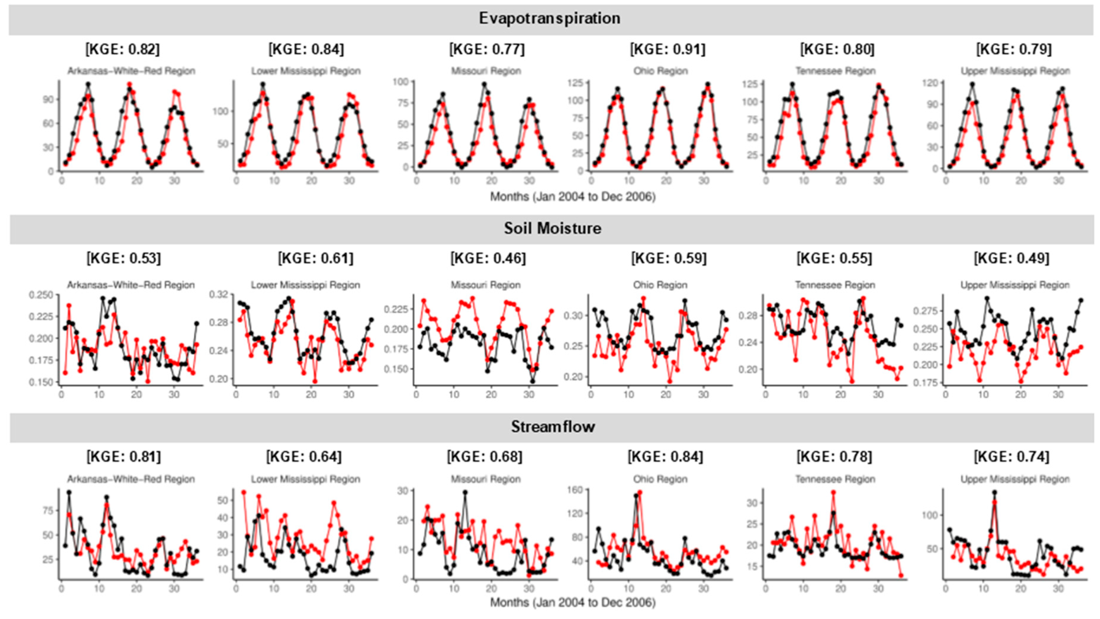
We first validate the Noah-MP hydrologic model using results from the univariate calibration cases (ET, SM, and SF) for the validation period of 2005 and 2006 (Figure 2). We then quantify the impact of univariate calibration on the representation of water balance components other than the one considered for calibration. Finally, we test the effectiveness of multivariate calibration for overcoming the drawbacks of univariate calibration and improving the simulation of the water balance components important for FEW nexus studies considered in this study (ET, SM, and SF).
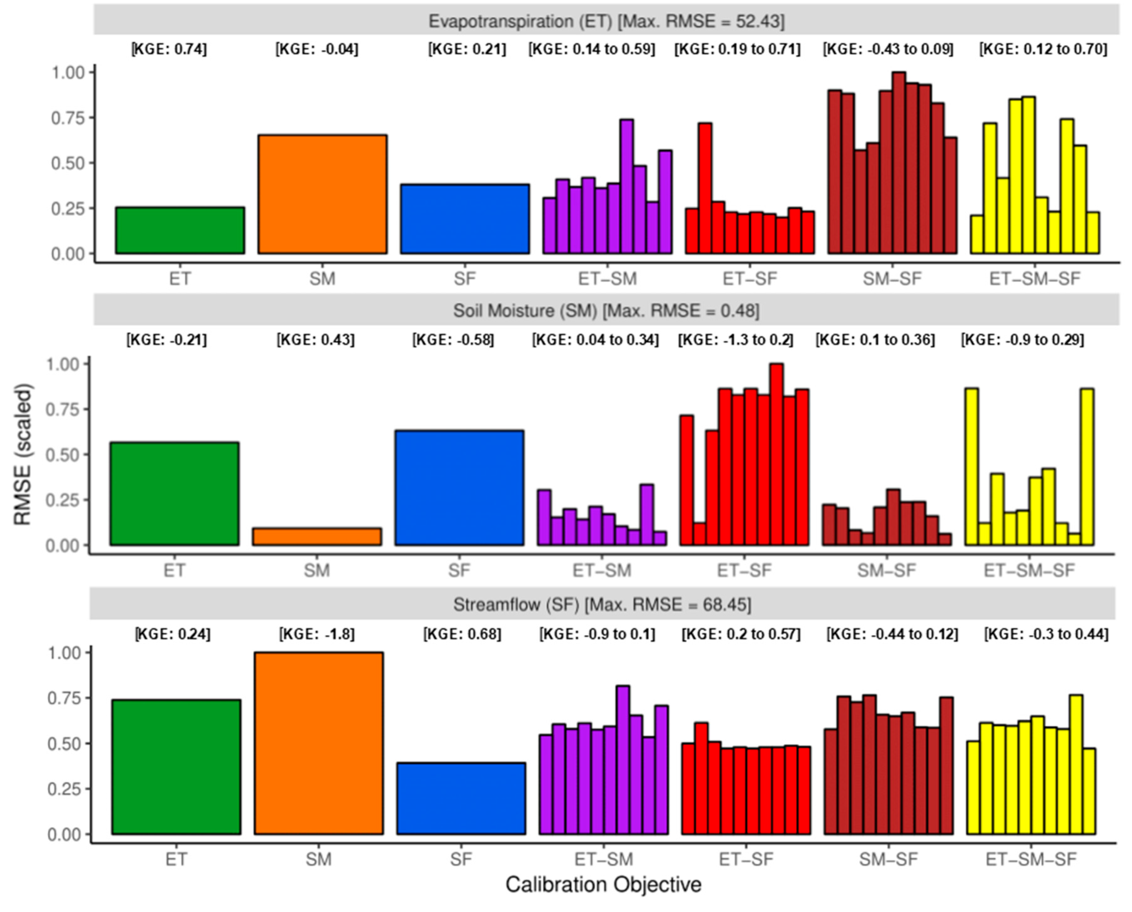
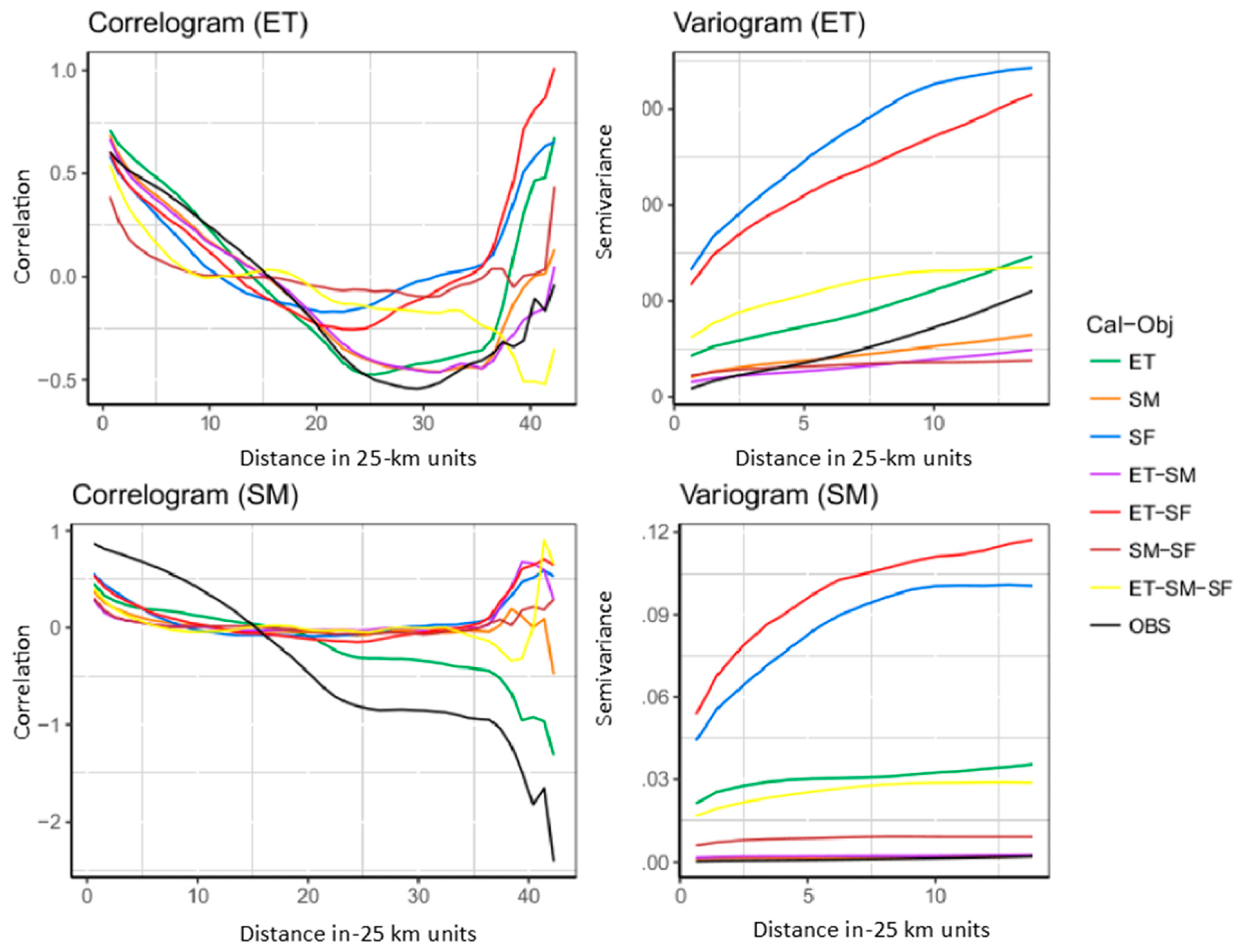
For the univariate and multivariate calibration cases, the temporal accuracy is analyzed using bar plots of the RMSE error metric of the basin-averaged monthly ET (top panel), SM (middle panel), and SF (bottom panel) for the seven calibrated scenarios (Figure 3). The RMSE values are scaled by the maximum RMSE among the seven calibration scenarios to allow comparison among the different fluxes that have different units. For the multivariate calibration scenarios (ET–SM, ET–SF, SM–SF, and ET–SM–SF) ten samples are drawn from the Pareto front and the basin-average RMSE is calculated. Spatial scaled-RMSE plots (Figure 4), variograms, and correlograms (Figure 5) calculated for average ET and SM values at each grid cell are used to quantify the effect of calibration on the spatial accuracy of ET and SM. For the multivariate calibration cases, the point that best represents the trade-off between the objectives was selected from the Pareto front to plot the correlograms and variograms. The equations used to calculate the variograms and correlograms are presented in Appendix B.

3. Results

3.1. Validation of the Noah-MP Hydrologic Model

The Noah-MP model is calibrated for 2004 and the simulated ET, SM, and SF results are validated for 2005 and 2006. A time comparison of observed and simulated monthly ET, SM, and SF are presented for the six HUC-2 sub catchments (Figure 2). We also present the corresponding Kling-Gupta Efficiency (KGE) values in each panel of Figure 2. When the Noah-MP model is calibrated with GLEAM ET (top panel), it is evident that the model performs very well in simulating the observed ET values and seasonality. The results are consistent across the six HUC-2 hydrologic regions and also between calibration (first 12 data points) and validation time periods (remaining 24 data points). Much higher variance is observed in the SM results when the Noah-MP model is calibrated with ESA–CCI soil moisture (middle panel). The simulated soil moisture for the Arkansas-White-Red, Lower Mississippi, Ohio, and Tennessee regions are consistent with observed SM values for the top soil layer. For these regions, the seasonality of soil moisture seen in the observations are well represented, with the last six months of 2006 in the Tennessee region (middle panel, fifth column) and the first few months of 2004 in the Arkansas-White-Red region (middle panel, first column) being the exceptions. In the Missouri region (middle panel, third column), the model simulates the observed seasonality but is unable to capture the absolute quantities of SM perfectly. In the Upper Mississippi region (middle panel, sixth column), the model struggles to simulate the timing of both the peaks and the troughs seen in the observed SM. The results for streamflow simulated by SF-calibrated Noah-MP model present a more complex picture (bottom panel). It is seen that the model generally performs well for the Arkansas-White-Red, Ohio, Tennessee, and Upper Mississippi regions. However, like soil moisture results, there are some inconsistencies in simulating the seasonality of the last six months of 2006, especially in Arkansas-White-Red (bottom panel, first column) and the Upper Mississippi (bottom panel, sixth column) regions. The model also performs well for the first 20 months in the Lower Mississippi and Missouri regions, but it seems to peak earlier (in 2006) than observed in the former while overestimating the runoff by a significant amount (months 20 to 27) in the latter. The KGE values are also very high for all the water balance components considered. In summary, it is seen that when the model is calibrated with the water balance component of interest (ET, SM, or SF) it can simulate the component with a reasonable degree of accuracy. The validation results also provide evidence for the use of one year of data for calibration, as the discovered parameter sets.

3.2. Univariate Calibration

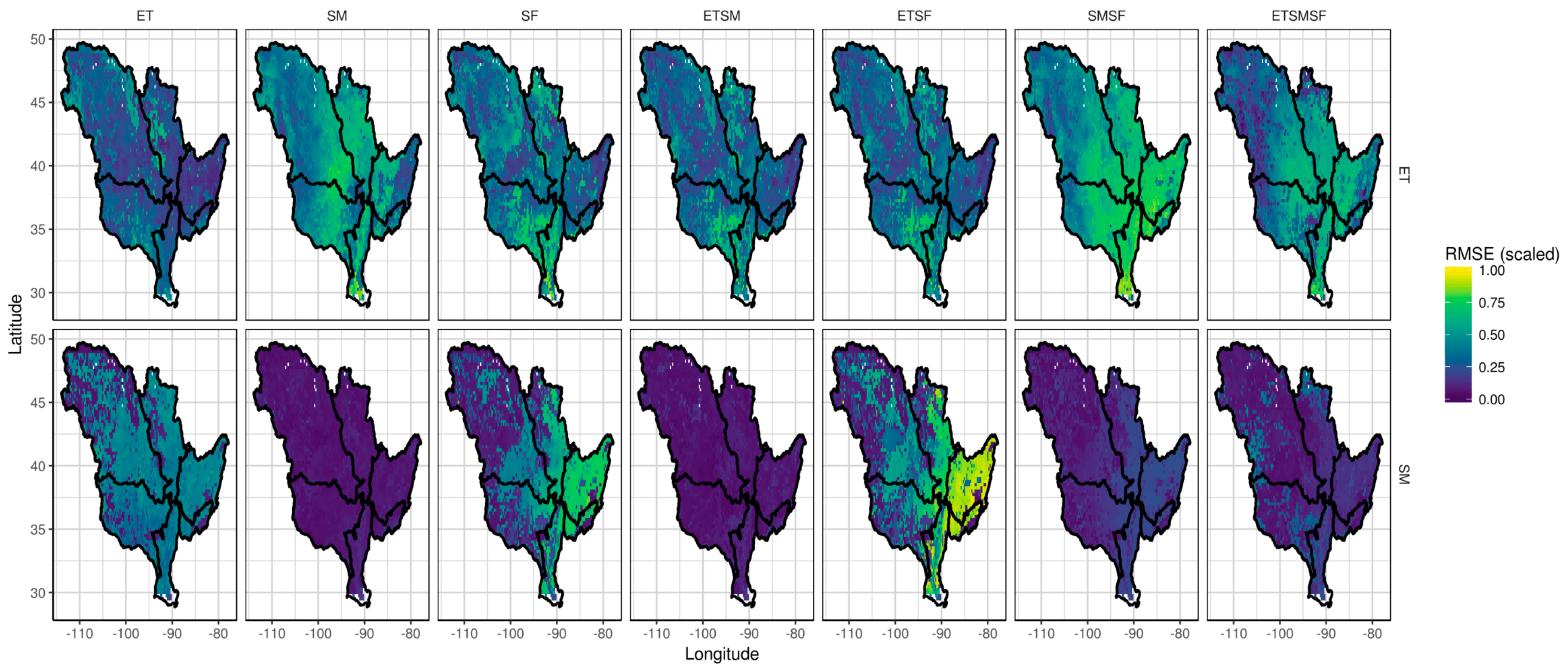
We first address the research question: does calibration of a distributed hydrologic model with a sparse network of streamflow gauges adversely affect ET and SM? From the bottom panel of Figure 3, it is clear that for SF, the model performs best when the calibration objective is SF (blue bar). Comparing the SF-calibrated ET with ET-calibrated ET (top panel, green) and SF-calibrated SM with SM-calibrated SM (middle panel, orange), it is also evident that this increased accuracy in SF comes at the cost of reduced accuracy in simulating ET (top panel, blue) and SM (middle panel, blue). The trade-off in SM accuracy is relatively higher compared to the reduction in ET performance. When the Noah-MP model is calibrated with only SF, the spatial representation of ET and SM is adversely affected (column three in Figure 4) when compared with ET-calibrated ET (first row, first column) and SM-calibrated SM (second row, second column). While the model seems to perform worse in the Lower Mississippi and Arkansas-White-Red sub-catchments for ET, the problem regions for SM seem to be the Ohio and Tennessee regions (both wet regions). The problems in the spatial structure of SF-calibrated ET and SM are clearer in the correlogram and variogram of ET and SM (Figure 5). For simulation of the ET variable, the correlogram of SF-calibrated ET (blue) matches the observed correlogram (black) up to a distance of 20 grid cells but significantly deviates after that. The variogram of SF-calibrated ET (blue) shows a much higher deviation from the observed variogram (black) with semivariance values between 300 and 400 compared to the observed range of 20 to 200. For SM, both the correlogram and the variogram of SF-calibrated SM (blue lines) exhibit significant deviations from the observations.
Next, we extend the analysis presented above to test whether calibration of hydrologic models with just one water balance component, in general, adversely affects the simulation of other water balance components. From Figure 3, it is fairly evident that accurate representation of any one component (ET, SM, or SF) comes at the cost of degrading the accurate representation of other water balance components. For example, ET-calibrated ET (top panel, green) has the least RMSE but corresponding SM (middle panel, green) is much higher compared to SM-calibrated SM (middle panel, orange). Also the SF simulated from ET-calibrated model is worse than SF-calibrated SF. The same conclusion can be drawn for SM. This fact is reflected in the spatial RMSE plot (Figure 4) as well, where ET-calibrated ET (first row, first column) shows good performance across the Mississippi river basin but the corresponding SM (second row, first column) performs poorly compared to SM-calibrated SM (second row, second column). The variogram of ET (Figure 5) shows that ET-calibrated ET (green lines) closely follows the observed correlogram and variograms (black lines) but the corresponding ET-calibrated SM shows significant deviation from the observed SM variogram. The correlogram of SM paints a slightly different picture, with ET-calibrated SM (green) seemingly better than SM-calibrated SM. This could be because of the nature of ESA–CCI soil moisture, which has a number of missing values due to the fact that there are a number of days in which the satellite does not pass over certain areas of the Mississippi basin, perhaps leading to erroneous spatial representation. However, we note that the spatial RMSE map of SM-calibrated SM (orange) is very close to the observed variogram (black) but this comes at the cost of reducing the accuracy of SM-calibrated ET. Barring the discrepancy in the correlogram of SM, we see that univariate calibration adversely affects the spatial and temporal accuracy of water balance not considered for calibration.

3.3. Multivariate Calibration

Can multivariate calibration help overcome the drawbacks of univariate calibration? We first analyze whether including ET and/or SM along with SF in calibration helps preserve the accuracy of both SF and ET and/or SM. When only ET is considered along with SF (ET–SF calibration case), some of the ET–SF-calibrated SF RMSE values (red bars, bottom panel, Figure 3) are slightly worse than SF-calibrated ET (blue bar, bottom panel) but the corresponding ET–SF-calibrated ET values (red bard, top panel) are considerably lesser than SF-calibrated ET values (blue bar, top panel). This shows that multivariate calibration (in this case ET–SF) trades-off accuracy in simulation of SF to improve the accuracy of ET. However, as expected, the lack of consideration of SM in the calibration results in a much higher RMSE value for the corresponding ET–SF-calibrated SM (red bars, middle panel). The inclusion of ET in calibration also seems to have improved the spatial RMSE, especially in the Missouri region of other Mississippi basin (first row, fifth column, Figure 4) compared to just SF-calibrated ET (first row, third column). The improvement in the RMSE values is not reflected in either the correlogram or the variogram of ET–SF-calibrated ET (red line, top panel, Figure 5). However, note that the correlograms and variograms are calculated for just one point in the Pareto front. It is safe to assume that there may be points on the Pareto front that could perform better as far as the correlogram or variogram is concerned. When only SM is included with SF, accuracy in SF simulation is traded for better simulation of SM. This is clearly evident in Figure 3, where all RMSE values of SM–SF-calibrated SF (brown bars, bottom panel) are worse than SF-calibrated SF (blue bar, bottom panel) but the corresponding SM–SF-calibrated SM (brown bars, middle panel) simulations perform much better than SF-calibrated SM (blue bar, middle panel). As seen before, this improved performance in SM comes at the cost of a slight reduction in SF accuracy, but the accuracy in ET suffers substantially (brown bars, top panel, Figure 3). The spatial RMSE plots, correlograms, and variograms paint a similar picture. Across the Mississippi basin, SM–SF-calibrated SM (second row, sixth column, Figure 4) performs much better than just SF-calibrated SM (second row, third column) but slightly worse than the SM-calibrated SM (second row, second column).
When both ET and SM are included with SF in calibrated (ET–SM–SF case), the derived Pareto surface has points which trade-offs, within acceptable limits, the accuracy in SF for better simulation of both ET and SM. In Figure 3, most RMSE values of ET–SM–SF-calibrated SF (yellow bars, bottom panel) are worse than SF-calibrated SF (blue bar, bottom panel) but some of the corresponding RMSE values for ET and SM are much better (in particular, the sixth yellow bar in top and middle panel). This improvement is more evident in the spatial RMSE plot (Figure 4) in which both the ET–SM–SF-calibrated ET (first row, last column) and ET–SM–SF-calibrated SM (second row, last column) show improvements over SF-calibrated ET and SM (third column). In the variogram of ET (Figure 5), ET–SM–SF-calibrated ET (yellow line) shows improvement over SF-calibrated ET (blue line) and even ET–SF-calibrated ET (red line). The SM variogram shows similar improvement. Although this analysis of results has been carried out from the perspective of SF, the conclusions drawn for SF hold true for both ET and SM. In other words, multivariate calibration can discover parameter sets which can simulate all the water balance components (in this case ET, SM, and SF) to a reasonable degree of accuracy, unlike univariate calibration.

4. Discussion

The inadequacy of calibrating hydrologic models with only SF for FEW nexus studies is clear from the results of our study. SF-calibration not only affects the basin-averaged values of other components such as ET or SM, but also, more importantly, results in an improper spatial representation of ET and SM. This behavior of hydrologic models, wherein the parameters are overfitted to accurately simulate only streamflow, is well-known. Several studies have shown that streamflow, being an integrative response of the entire watershed, cannot adequately inform the spatial representation of ET and SM [37,38]. Recent studies have shown that using the spatial structure of ET and SM from remote sensing data along with streamflow data in calibration can produce physically consistent estimates of all the components [9,39,40]. In this regard, our study agrees with the findings of the hydrologic modeling community, with the spatial RMSE plots (Figure 4), variograms, and correlograms (Figure 5) showing that considering ET and SM moisture improves their spatial structure. However, in this study, we go beyond quantifying and addressing the impacts of only streamflow calibration by also focusing on the ill-effects of univariate calibration, in general, for hydrologic and FEW nexus studies. In doing so, we find that using soil moisture data for calibration has the most adverse impact on the accuracy of the other variables. This could be due to the fact that the parameters that are sensitive to soil moisture may not be sensitive to other variables. This is in contrast to the findings of [7], who found out that incorporating near-surface remote sensing-based estimates of soil moisture and streamflow in hydrologic model calibration positively impacts streamflow simulation. On the other hand, ET-calibration yields much better results for SF and ET simulation but the corresponding SM representation is poor. This is expected as the parameters which influence SF also impact ET (more than SM). This highlights the need for better, physically interpretable, parameterization of hydrologic models.
Multivariate calibration of hydrologic models is generally carried out by combining different hydrologic variables into a single objective function by using weights [9,40,41]. Such an approach makes it difficult to analyze the trade-offs in accuracy among the different variable involved. In this study, we present a Pareto optimality-based calibration strategy for multivariate calibration which helps in systematically quantifying the improvements in simultaneously simulating multiple water balance components. This is especially true for FEW nexus studies which would need more than just ET, SM, and SF variables, and the approach presented here can help in systematically introducing new datasets such as total water storage change and groundwater information, among others. The advantage of such an approach is apparent in Figure 3, where the progressive introduction of variables (for example, SF, ET–SF, and ET–SM–SF) changes the RMSE of different variables of interest. These changes can be systematically analyzed for a particular hydrologic model (in this case, Noah-MP) and relevant calibration strategies for the specific FEW nexus study can be devised. For the Noah-MP model used in this study, the progressive inclusion of different variables lead to the following calibration strategies for different FEW nexus studies:
  • ET: If the nexus study only requires ET as the primary input (for example, calculation of water demand), then calibration of a hydrologic model using only observed ET gives the best results in terms of spatial and temporal accuracy. However, increased accuracy in ET comes at the cost of degrading SM and SF estimates. In the absence of SF estimates, calibration with observed ET offers the best alternative for reliably simulating SF [42,43].
  • SM: Calibration of a hydrologic model with SM observations improves SM simulations significantly at considerable cost to the accuracy of both ET and SF simulations. Based on the results of this study, SM-calibration is not a viable variable for FEW nexus studies which need either water availability (SF) or water use (ET) information. SM-calibration maybe required for FEW studies in drought-affected regions where water availability is government by SM.
  • SF: Using a sparse network of streamflow gages for calibration adversely affects the spatio-temporal accuracy of ET and SM. If no ET observations are available, then SF is a viable alternative for reliably simulating mean ET over the basin but not the spatial patterns which are necessary for most FEW nexus studies.
  • ET–SM: Including ET and SM together in calibration not only improves the simulations of ET and SM but also has a positive impact on SF estimates compared to univariate calibration cases. This scenario exhibits the advantages of combining state-of-art remote sensing-based estimates of hydrologic variables with models for FEW nexus studies, especially for FEW nexus studies in data-scarce regions.
  • ET–SF: Incorporating both ET and SF in calibration trades accuracy in SF simulation to improve ET estimates compared to univariate SF calibration. If ET and SF variables are needed for the FEW study, then this scenario is the best calibration strategy. However, combining and ET and SF does not improve soil moisture simulation (even compared to univariate ET or SF calibration).
  • SM–SF: In the absence of ET observations or estimates, SM and SF are seen to be poor alternatives. Therefore this calibration scenario cannot be used for FEW nexus studies that require ET. However, this strategy can be used in nexus studies in regions which suffer from episodic droughts where both SM and SF are needed to quantify water availability.
  • ET–SM–SF: Incorporating all the water balance components (ET, SM, SF) for calibration provides the best compromise solution to preserve the accuracies in simulating each of the three components.
Finally we discuss whether using remotely sensed ET and SM for calibration lead to reliable streamflow simulations. This is important for FEW nexus studies in data-scarce regions where in situ measurements of SF are not available. If better SF simulation is the sole objective, combining ET and SM for calibration (ET–SM-calibrated case) produces slightly better results than just considering ET (compare purple and green bars in bottom panel of Figure 3). However, if the intention of the model is to preserve the accuracy of other variables (ET and SM), as is the case in FEW nexus studies, then combining both ET and SM in a multivariate calibration setup produces better results (compare purple, green, and orange bars in top and bottom panel). By comparing ET-calibrated SF (green bar, bottom panel) and SM-calibrated SF (orange bar, bottom panel), it is clear that ET can inform SF simulation better than SM. In most large scale FEW nexus studies it is important to simulate the spatial distribution of ET and SM with reasonable accuracy. For this purpose, combining both ET and SM in calibration produces much better spatial structure rather than univariate calibration (compare 4th column with first and second columns in Figure 4, also purple lines with black lines in Figure 5).

5. Conclusions

In this study, we presented the results of a calibration experiment in the Mississippi river basin aimed at understanding the applicability of large scale spatially distributed hydrologic models for FEW nexus studies. The primary objective of the study was to quantify the impact of using estimates of a single water balance component on the other water balance components. For this, we analyzed the results from seven different univariate (ET, SM, and SF) and multivariate calibration (ET–SM, ET–SF, SM–SF, and ET–SM–SF) scenarios. We have shown that the univariate calibration does indeed affect the simulation of water balance components that are not included in calibration, and as such is not suitable for FEW nexus studies. In addition, we have shown that a trade-off relationship exists among the simulated water balance components, which is best characterized by a Pareto front or surface. This led us to use multivariate calibration as an approach to improve the applicability of hydrologic models for FEW nexus studies.
Although the theoretical underpinnings of multivariate calibration have been well-established over the last two decades, the applicability of these methods was hindered by the lack of estimates of hydrologic variables other than streamflow. The availability of remote sensing data and powerful optimization algorithms enabled us to quantify the trade-off relationship among accurate simulation of different water balance components. Our results show that multivariate calibration approach used in this study has the potential in improving hydrologic models for FEW nexus studies. With multivariate calibration, the hydrologic models are able to (1) accurately represent the spatial structure of the hydrologic variables other than streamflow (ET and SM) and (2) preserve the accuracy with which streamflow is simulated. In addition, the study adds to an increasing body of evidence in favor of using satellite-based remote sensing data for improving hydrologic models using different approaches such as calibration and data assimilation. This is especially important within the framework of food–energy–water nexus studies.
Finally, we briefly enumerate the limitations of the study and possible future directions. The conclusions drawn above are a result of the chosen hydrologic model (Noah-MP), physics options, parameters, input data, and meteorological forcing. For a different setup the trade-offs may have different characteristics. However, the multivariate calibration approach of combining different remote sensing-based dataset can be applied for any type of hydrologic model and FEW nexus study. Future work involves using the Gravity Recovery and Climate Experiment (GRACE)-based estimates of total water storage (TWS), which could perform better than just near-surface soil moisture (top 5 cm) used in the study. Also, we have considered only a sparse network of streamflow gauges, primarily to mimic large scale FEW nexus studies which deal with data sparsity, but it is worthwhile to explore if a dense network of streamflow gauges could lead to better ET and SM simulations.

Author Contributions

Conceptualization, A.K.; methodology, A.K.; formal analysis, A.K.; investigation, A.K. and M.G.; resources, M.G.; data curation, A.K.; writing—original draft preparation, A.K.; writing—review and editing, A.K. and M.G.; visualization, A.K.; supervision, M.G.; funding acquisition, M.G. All authors have read and agreed to the published version of the manuscript.

Funding

We acknowledge funding support from the NASA Applied Sciences Water Resources Application Grant # NNX15AC33G.

Acknowledgments

We thank Jasper Vrugt for help with AMALGAM algorithm. We also thank Shawn L. Mattot for help with OSTRICH optimization software. The GLEAM ET dataset has been sourced from www.gleam.eu, ESA–CCI soil moisture from www.esa-soilmoisture-cci.org, Ameriflux ET from ameriflux.lbl.gov, and TAMU soil moisture from http://soilmoisture.tamu.edu/Data/. NASA’s Land Information System is sourced from https://lis.gsfc.nasa.gov./ OSTRICH software is sourced from http://www.eng.buffalo.edu/lsmatott/Ostrich/. AMALGAM software is available at http://faculty.sites.uci.edu/jasper/software/.

Conflicts of Interest

The authors declare no conflicts of interest.

Appendix A

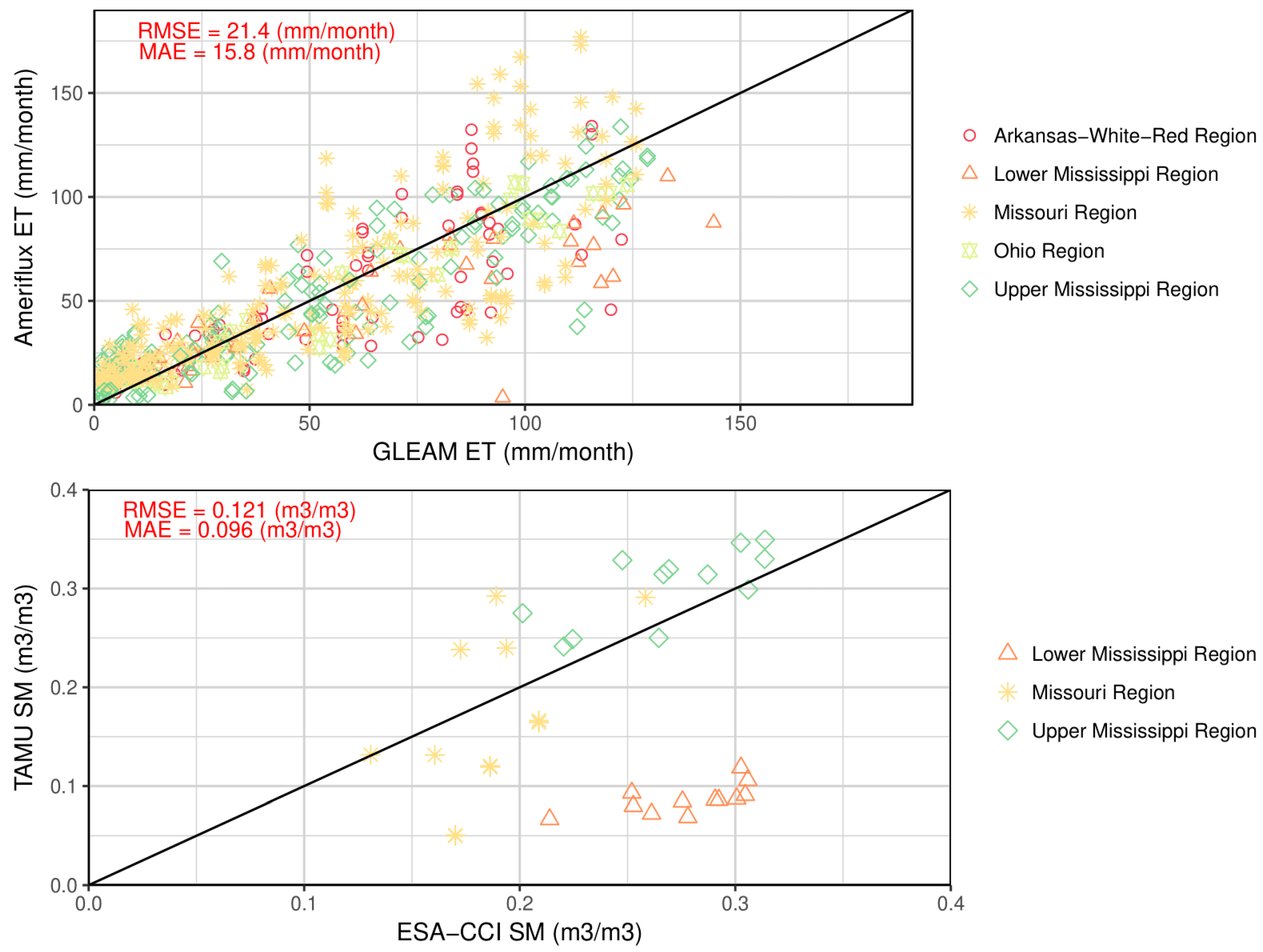
As remote sensing-based hydrologic datasets exhibit large uncertainty [44], we evaluate the chose ET and SM datasets with ground-based measurements. We compare the GLEAM estimates with ground-based flux tower data from the Ameriflux network (https://ameriflux.lbl.gov/). Results of the evaluation show that GLEAM can represent the ET flux in all the sub-basins to a fair degree of accuracy for the year 2004 (Figure A1 (top)). The RMSE of GLEAM data is 21.4 mm/month. We compare the remote sensing-based ESA–CCI SM dataset with near-surface soil moisture measurements from the TAMU North American Soil Moisture Database (NASMDB) [45]. The scatter plot (Figure A1 (bottom)) shows that the remote sensing data underestimates observed soil moisture in the Lower Mississippi Region. The RMSE value for ESA–CCI SM is 0.12 m3/m3. We note that for the study period SM data from in situ sensors were available only for 3 of the 6 sub-basins.
Figure A1. Scatter plots of GLEAM ET vs. Ameriflux measurements (top panel) and ESA–CCI soil moisture vs. TAMU NASMDB measurements (bottom panel) for 2004. RMSE and the Mean Absolute Error (MAE) values are indicated in red.
Remotesensing 12 00599 g0a1

Appendix B

The correlogram presented in Figure 5 is calculated using the following equation.
c ( d ) =   1 n ( d ) i = 1 n ( d ) [ ( z ( x i + d )   z ¯ ) ( z ( x i )   z ¯ ) ]
where c ( d ) , is he spatial autocorrelation, which is a function of distance d between two data points (in this study we consider ET and SM), z ( x i + d ) and z ( x i ) . z ¯ is the mean of the data considered for determining the correlogram (ET or SM), n(d) is the total number of data pairs of ET or SM.
The semivariance in the variogram presented in Figure 5 for ET and SM is calculated using the following equation
γ ( d ) =   1 2 n ( d ) i = 1 n ( d ) [ z ( x i + d ) z ( x i ) ] 2
where γ ( d ) , is the semivariance, which is a function of the distance d between two data points (ET or SM), z ( x i + d ) and z ( x i ) . n(d) is the total number of data pairs of ET or SM.

References

  1. D’Odorico, P.; Davis, K.F.; Rosa, L.; Carr, J.A.; Chiarelli, D.; Dell’Angelo, J.; Gephart, J.; MacDonald, G.K.; Seekell, D.A.; Suweis, S.; et al. The Global Food-Energy-Water Nexus. Rev. Geophys. 2018, 56, 456–531. [Google Scholar] [CrossRef]
  2. Mcnally, A.; Mccartney, S.; Ruane, A.C.; Mladenova, I.E.; Mcnally, A. Hydrologic and Agricultural Earth Observations and Modeling for the Water-Food Nexus. Front. Environ. Sci. 2019, 7, 23. [Google Scholar] [CrossRef] [Green Version]
  3. McCallum, I.; Montzka, C.; Bayat, B.; Kollet, S.; Kolotii, A.; Kussul, N.; Lavreniuk, M.; Lehmann, A.; Maso, J.; Mazzetti, P.; et al. Developing food, water and energy nexus workflows. Int. J. Digit. Earth 2020, 13, 299–308. [Google Scholar] [CrossRef]
  4. Momblanch, A.; Papadimitriou, L.; Jain, S.K.; Kulkarni, A.; Ojha, C.S.P.; Adeloye, A.J.; Holman, I.P. Untangling the water-food-energy-environment nexus for global change adaptation in a complex Himalayan water resource system. Sci. Total Environ. 2019, 655, 35–47. [Google Scholar] [CrossRef]
  5. Alam, S.; Gebremichael, M.; Li, R. Remote Sensing-Based Assessment of the Crop, Energy and Water Nexus in the Central Valley, California. Remote Sens. 2019, 11, 1701. [Google Scholar] [CrossRef] [Green Version]
  6. Koppa, A.; Gebremichael, M.; Yeh, W.W.-G. Multivariate calibration of large scale hydrologic models: The necessity and value of a Pareto optimal approach. Adv. Water Resour. 2019, 130, 129–146. [Google Scholar] [CrossRef]
  7. Wanders, N.; Bierkens, M.F.P.; de Jong, S.M.; de Roo, A.; Karssenberg, D. The benefits of using remotely sensed soil moisture in parameter identification of large-scale hydrological modelss. Water Resour. Res. 2014, 50, 6874–6891. [Google Scholar] [CrossRef] [Green Version]
  8. Immerzeel, W.W.; Droogers, P. Calibration of a distributed hydrological model based on satellite evapotranspiration. J. Hydrol. 2008, 349, 411–424. [Google Scholar] [CrossRef]
  9. Zink, M.; Mai, J.; Cuntz, M.; Samaniego, L. Conditioning a Hydrologic Model Using Patterns of Remotely Sensed Land Surface Temperature. Water Resour. Res. 2018, 54, 2976–2998. [Google Scholar] [CrossRef]
  10. López, P.L.; Sutanudjaja, E.H.; Schellekens, J.; Sterk, G.; Bierkens, M.F.P. Calibration of a large-scale hydrological model using satellite-based soil moisture and evapotranspiration products. Hydrol. Earth Syst. Sci. 2017, 21, 3125–3144. [Google Scholar] [CrossRef] [Green Version]
  11. Beven, K.; Freer, J. Equifinality, data assimilation, and uncertainty estimation in mechanistic modelling of complex environmental systems using the GLUE methodology. J. Hydrol. 2001, 249, 11–29. [Google Scholar] [CrossRef]
  12. Beven, K. Searching for the Holy Grail of scientific hydrology: Qt = (S, R, Δt) A as closure. Hydrol. Earth Syst. Sci. 2006, 10, 609–618. [Google Scholar] [CrossRef] [Green Version]
  13. Beven, K.; Binley, A. The future of distributed models: Model calibration and uncertainty prediction. Hydrol. Process. 1992, 6, 279–298. [Google Scholar] [CrossRef]
  14. Gupta, H.V.; Sorooshian, S.; Yapo, P.O. Toward improved calibration of hydrologic models: Multiple and noncommensurable measures of information. Water Resour. Res. 1998, 34, 751–763. [Google Scholar] [CrossRef]
  15. Lettenmaier, D.P.; Alsdorf, D.; Dozier, J.; Huffman, G.J.; Pan, M.; Wood, E.F. Inroads of remote sensing into hydrologic science during the WRR era. Water Resour. Res. 2015, 51, 7309–7342. [Google Scholar] [CrossRef]
  16. Cai, X.; Yang, Z.L.; David, C.H.; Niu, G.Y.; Rodell, M. Hydrological evaluation of the Noah-MP land surface model for the Mississippi River Basin. J. Geophys. Res. 2014, 119, 23–38. [Google Scholar] [CrossRef]
  17. Martens, B.; Miralles, D.G.; Lievens, H.; Van Der Schalie, R.; De Jeu, R.A.M.; Fernández-Prieto, D.; Beck, H.E.; Dorigo, W.A.; Verhoest, N.E.C. GLEAM v3: Satellite-based land evaporation and root-zone soil moisture. Geosci. Model Dev. 2017, 10, 1903–1925. [Google Scholar] [CrossRef] [Green Version]
  18. Koppa, A.; Gebremichael, M. A Framework for Validation of Remotely Sensed Precipitation and Evapotranspiration Based on the Budyko Hypothesis. Water Resour. Res. 2017, 53, 8487–8499. [Google Scholar] [CrossRef]
  19. Dorigo, W.; Wagner, W.; Albergel, C.; Albrecht, F.; Balsamo, G.; Brocca, L.; Chung, D.; Ertl, M.; Forkel, M.; Gruber, A.; et al. ESA CCI Soil Moisture for improved Earth system understanding: State-of-the art and future directions. Remote Sens. Environ. 2017, 203, 185–215. [Google Scholar] [CrossRef]
  20. Niu, G.Y.; Yang, Z.L.; Mitchell, K.E.; Chen, F.; Ek, M.B.; Barlage, M.; Kumar, A.; Manning, K.; Niyogi, D.; Rosero, E.; et al. The community Noah land surface model with multiparameterization options (Noah-MP): 1. Model description and evaluation with local-scale measurements. J. Geophys. Res. Atmos. 2011, 116. [Google Scholar] [CrossRef] [Green Version]
  21. Kumar, S.V.; Peters-Lidard, C.D.; Tian, Y.; Houser, P.R.; Geiger, J.; Olden, S.; Lighty, L.; Eastman, J.L.; Doty, B.; Dirmeyer, P.; et al. Land information system: An interoperable framework for high resolution land surface modeling. Environ. Model. Softw. 2006, 21, 1402–1415. [Google Scholar] [CrossRef]
  22. Cuntz, M.; Mai, J.; Samaniego, L.; Clark, M.; Wulfmeyer, V.; Branch, O.; Attinger, S.; Thober, S. The impact of standard and hard-coded parameters on the hydrologic fluxes in the Noah-MP land surface model. J. Geophys. Res. 2016, 121, 10676–10700. [Google Scholar] [CrossRef]
  23. Ball, J.T.; Woodrow, I.E.; Berry, J.A. A Model Predicting Stomatal Conductance and its Contribution to the Control of Photosynthesis under Different Environmental Conditions. In Progress in Photosynthesis Research; Springer: Dordrecht, The Netherlands, 1987; pp. 221–224. [Google Scholar] [CrossRef]
  24. Chen, F.; Janjić, Z.; Mitchell, K. Impact of atmospheric surface-layer parameterizations in the new land-surface scheme of the NCEP mesoscale Eta model. Bound.-Layer Meteorol. 1997, 85, 391–421. [Google Scholar] [CrossRef]
  25. Niu, G.Y.; Yang, Z.L.; Dickinson, R.E.; Gulden, L.E.; Su, H. Development of a simple groundwater model for use in climate models and evaluation with Gravity Recovery and Climate Experiment data. J. Geophys. Res. Atmos. 2007, 112. [Google Scholar] [CrossRef]
  26. Niu, G.Y.; Yang, Z.L. Effects of frozen soil on snowmelt runoff and soil water storage at a continental scale. J. Hydrometeorol. 2006, 7, 937–952. [Google Scholar] [CrossRef]
  27. Yang, R.; Friedl, M.A. Modeling the effects of three-dimensional vegetation structure on surface radiation and energy balance in boreal forests. J. Geophys. Res. D Atmos. 2003, 108. [Google Scholar] [CrossRef]
  28. Verseghy, D.L.; McFarlane, N.A.; Lazare, M. Class—A Canadian land surface scheme for GCMS, II. Vegetation model and coupled runs. Int. J. Climatol. 1993, 13, 347–370. [Google Scholar] [CrossRef]
  29. Jordan, R. A One-Dimensional Temperature Model for a Snow Cover: Technical Documentation for SNTHERM.89; Cold Regions Research and Engineering Laboratory: Hanover, NH, USA, 1991. [Google Scholar]
  30. Tolson, B.A.; Shoemaker, C.A. Dynamically dimensioned search algorithm for computationally efficient watershed model calibration. Water Resour. Res. 2007, 43. [Google Scholar] [CrossRef]
  31. Duan, Q.Y.; Gupta, V.K.; Sorooshian, S. Shuffled complex evolution approach for effective and efficient global minimization. J. Optim. Theory Appl. 1993, 76, 501–521. [Google Scholar] [CrossRef]
  32. Vrugt, J.A.; Robinson, B.A. Improved evolutionary optimization from genetically adaptive multimethod search. Proc. Natl. Acad. Sci. USA 2007, 104, 708–711. [Google Scholar] [CrossRef] [PubMed] [Green Version]
  33. Storn, R.; Price, K. Differential Evolution—A Simple and Efficient Heuristic for Global Optimization over Continuous Spaces. J. Glob. Optim. 1997, 11, 341–359. [Google Scholar] [CrossRef]
  34. Kennedy, J.; Eberhart, R.C.; Shi, Y.; Jacob, C.; Koza, J.R.; Iii, F.H.B.; Andre, D.; Keane, M. Swarm Intelligence. The Morgan Kaufmann Series in Evolutionary Computation; Morgan Kaufmann: Burlington, MA, USA, 2001; ISBN 1558605959. [Google Scholar]
  35. Haario, H.; Saksman, E.; Tamminen, J. An adaptive Metropolis algorithm. Bernoulli 2001, 7, 223–242. [Google Scholar] [CrossRef] [Green Version]
  36. Deb, K.; Pratap, A.; Agarwal, S.; Meyarivan, T. A fast and elitist multiobjective genetic algorithm: NSGA-II. IEEE Trans. Evol. Comput. 2002, 6, 182–197. [Google Scholar] [CrossRef] [Green Version]
  37. Mendoza, P.A.; Clark, M.P.; Barlage, M.; Rajagopalan, B.; Samaniego, L.; Abramowitz, G.; Gupta, H. Are we unnecessarily constraining the agility of complex process-based models? Water Resour. Res. 2015, 51, 716–728. [Google Scholar] [CrossRef]
  38. Samaniego, L.; Kumar, R.; Attinger, S. Multiscale parameter regionalization of a grid-based hydrologic model at the mesoscale. Water Resour. Res. 2010, 46. [Google Scholar] [CrossRef] [Green Version]
  39. Stisen, S.; Koch, J.; Sonnenborg, T.O.; Refsgaard, J.C.; Bircher, S.; Ringgaard, R.; Jensen, K.H. Moving beyond run-off calibration-Multivariable optimization of a surface-subsurface-atmosphere model. Hydrol. Process. 2018, 32, 2654–2668. [Google Scholar] [CrossRef]
  40. Dembélé, M.; Hrachowitz, M.; Savenije, H.H.G.; Mariéthoz, G.; Schaefli, B. Improving the Predictive Skill of a Distributed Hydrological Model by Calibration on Spatial Patterns with Multiple Satellite Data Sets. Water Resour. Res. 2020, 56. [Google Scholar] [CrossRef]
  41. Rakovec, O.; Kumar, R.; Attinger, S.; Samaniego, L. Improving the realism of hydrologic model functioning through multivariate parameter estimation. Water Resour. Res. 2016, 52, 7779–7792. [Google Scholar] [CrossRef]
  42. Koppa, A.; Gebremichael, M.; Zambon, R.C.; Yeh, W.W.-G.; Hopson, T.M. Seasonal Hydropower Planning for Data-Scarce Regions Using Multimodel Ensemble Forecasts, Remote Sensing Data, and Stochastic Programming. Water Resour. Res. 2019, 55, 8583–8607. [Google Scholar] [CrossRef]
  43. Becker, R.; Koppa, A.; Schulz, S.; Usman, M.; aus der Beek, T.; Schüth, C. Spatially distributed model calibration of a highly managed hydrological system using remote sensing-derived ET data. J. Hydrol. 2019, 577, 123944. [Google Scholar] [CrossRef]
  44. Kidd, C.; Huffman, G. Global precipitation measurement. Meteorol. Appl. 2011, 18, 334–353. [Google Scholar] [CrossRef]
  45. Quiring, S.M.; Ford, T.W.; Wang, J.K.; Khong, A.; Harris, E.; Lindgren, T.; Goldberg, D.W.; Li, Z. The North American soil moisture database development and applications. Bull. Am. Meteorol. Soc. 2016, 97, 1441–1459. [Google Scholar] [CrossRef]
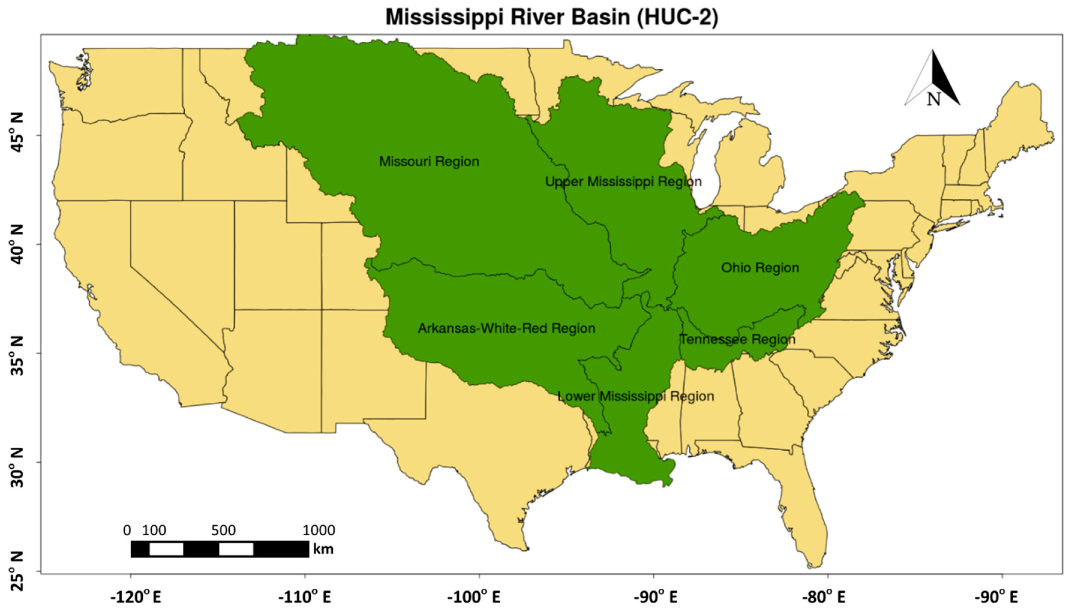
Figure 1. A map of the Mississippi basin showing the six USGS Hydrologic Unit Code (HUC)-2 basins.
Remotesensing 12 00599 g001
Figure 2. Time series plots of (1) top panel: Evapotranspiraton-calibrated (ET-calibrated) model ET (red) and the Global Land Evaporation Amsterdam Model (GLEAM) observed ET (black) in mm/month, (2) middle panel: Soil moisture-calibrated (SM-calibrated) model SM (red) and the European Space Agency–Climate Change Institute (ESA–CCI) observed SM (black) in m3/m3 and (3) bottom panel: Streamflow-calibrated (SF-calibrated) model SF (red) and observed Hydrologic Unit Code-2 (HUC-2) runoff (black) in mm/month for the six HUC-2 sub-catchments of the Mississippi basin. The first 12 months correspond to the calibration period of 2004 and the next 24 months correspond to validation years 2005 and 2006. The corresponding Kling-Gupta Efficiency (KGE) values are presented in each panel.
Remotesensing 12 00599 g002
Figure 3. Bar plots of scaled RMSE values of basin averaged monthly ET (top panel), SM (middle panel), and SF (bottom panel) when the Noah-MP model is calibrated with (1) ET, (2) SM, (3) SF, (4) ET–SM, (5) ET–SF, (6) SM–SF, and (7) ET–SM–SF as calibration objectives (x-axis in all three panels). RMSE values for ET, SM, and SF are scaled by the maximum RMSE across the seven calibration cases. The maximum values are provided in the header of each panel within square brackets. The multivariate calibration results are derived by taking 10 samples from different points on the Pareto fronts. We also present KGE values for each of the calibration cases above each barplot. For multivariate calibration cases, only the range of KGE values from the selected Pareto-optimal parameter sets are shown.
Remotesensing 12 00599 g003
Figure 4. Spatial plots of scaled RMSE values of ET (top panel) and SM (bottom panel) when the Noah-MP model is calibrated with (1) ET, (2) SM, (3) SF, (4) ET–SM, (5) ET–SF, (6) SM–SF, and (7) ET–SM–SF as calibration objectives.
Remotesensing 12 00599 g004
Figure 5. Correlogram and Variogram of ET (top panel) and SM (bottom panel) when the Noah-MP model is calibrated with (1) ET, (2) SM, (3) SF, (4) ET–SM, (5) ET–SF, (6) SM–SF, and (7) ET–SM–SF as calibration objectives.
Remotesensing 12 00599 g005
Table 1. Noah-MP (multi-parameterization) model physics options.
Model PhysicsSelected Physics Option
Vegetation modelUse table Leaf Area Index (4)
Canopy stomatal resistanceBall-Berry (1) [23]
Soil moisture factor for stomatal resistanceOriginal Noah (1) [24]
Runoff and groundwaterTOPMODEL with groundwater (1) [25]
Surface layer drag coefficientOriginal Noah (2) [24]
Frozen soil permeabilityLinear effects, more permeable (1) [26]
Radiation transferModified two-stream (1) [27]
Snow surface albedoCLASS (2) [28]
Rainfall and snowfall PartitioningJordan Scheme (1) [29]
Lower boundary of soil temperatureOriginal Noah (2) [24]
Snow and soil temperature time schemeSemi-implicit (1)
Super-cooled liquid waterNo iteration (1) [26]
The number in the brackets represents the internal Noah-MP model code for the selected physics option.
Table 2. Details of Noah-MP parameters used for calibration.
ParametersDescriptionSensitive VariableTotal ParametersUnitsMinimumMaximum
REFDKSurface runoff parameterSF1m/s1.4 × 10−66.5 × 10⁻⁶
REFKDTSurface runoff parameterSF1No Units1.05.0
BB1-BB12Exponent in the Brooks Corey EquationSF, ET12No Units0.512.0
MAXSMC1-MAXSMC12Soil porositySF, ET, SM12No units0.10.7
SATDK1-SATDK12Saturated hydraulic conductivitySF, SM12m/s2.0 × 10−67.0 × 10⁻²
Soil texture classes for BB, MAXSMC and SATDK (from 1 to 12): sand, loamy sand, sandy loam, silt loam, silt, loam, sandy clay loam, silt clay loam, clay loam, sandy clay, silty clay, and clay.