1. Introduction
Synthetic aperture radar (SAR) imagery is widely utilized in remote sensing because of its features of all-day, all weather and high-resolution [
1]. Additionally, digital elevation model (DEM) generation using high-resolution SAR images has become an important application.
DEM generation techniques based on SAR imagery can be roughly divided into two categories: interferometry [
2,
3] and radargrammetry [
4,
5]. For the interferometric configuration, the phase data is converted into height value [
6]. There are demanding requirements on system and experiment conditions. For example, it is necessary that two images of the same area should be acquired with slightly different incidence angles [
7].
The radargrammetric approach was first applied in 1950s [
8]. Compared with the interferometric approach, radargrammetry makes use of image intensity rather than phase information. It can be applied in images with varying incidence angles or varying aspect angles. Varying incidence angle is common in radargrammetric application, while varying aspect angles of SAR trajectory has potential to be explored for DEM generation with the emergence of multi-aspect imaging mode [
9]. Multi-aspect SAR refers to a wide angular aperture imaging mode that the radar beam always points to the center of the scene at different viewing aspect angles [
10]. That new imaging mode satisfies the increasing demand of finer observation, where some targets have to be studied from multi aspect angles. For example, circular SAR (CSAR) is one of the representative systems of multi-aspect SAR, which performs 360-degree observation [
11].
Multi-aspect images applied for DEM generation can also employ the conventional radargrammetric method. The traditional way is to find the imaging positions of the target on a correlation matched image pair formed on slant range plane or ground plane from different viewing angles [
12,
13]. Three-dimensional coordinates of the target are taken as unknown variables, and the coordinates of the target can be solved by solving the nonlinear equations listed according to the range-Doppler (RD) model [
14] or rational polynomial coefficient (RPC) model [
15]. The amount of computation of this process is high. From another point of view, authors try to find an estimated height with maximum correlation coefficient between two image patches for all possible height values at each resolution cell [
16]. However, massive correlation evaluation carried out along a set of height values at each resolution grid is time consuming.
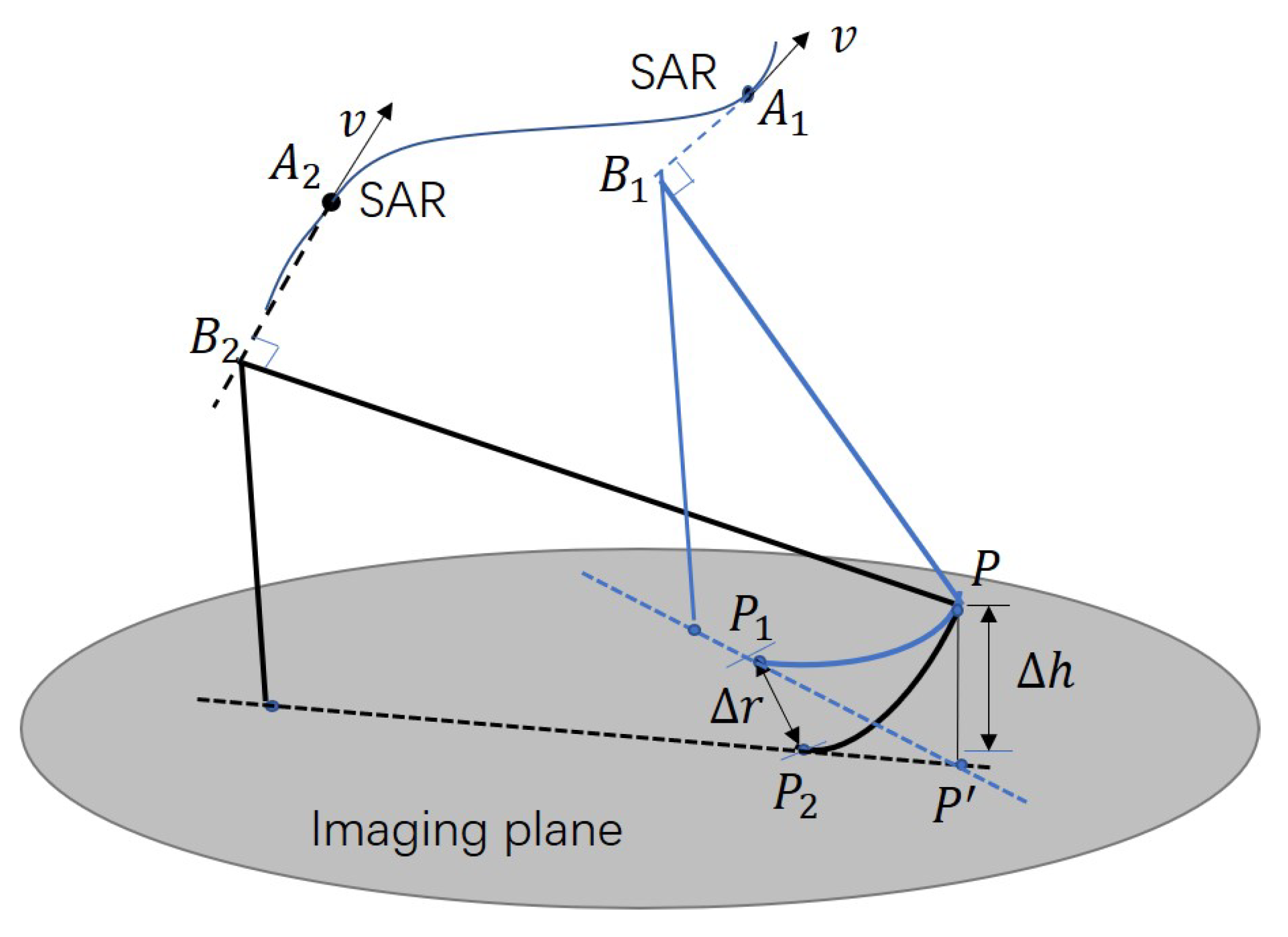
When radar images from different aspect angles are processed on the slant range plane, the imaging coordinate system of each image is different. However if multi-aspect images are all formed on the ground plane, images from different aspect angles are in the same coordinate system. In this case, height difference between true height of the target and imaging plane of fixed elevation is considered to be the only reason that causes imaging positions shift [
9]. If height of the imaging plane is not equal to the height of object, the imaging positions from different aspect angles will be different [
17]. Here we proposed a new DEM generation method for multi-aspect images generated on the ground plane. We derived the linear relationship between offset of imaging positions and height difference and deduced a scale factor to express it. Thus the offset between images from different aspect angles can be used to retrieve the elevation of the scene. So the solution to the RD equations in traditional procedure can be avoided.
CSAR images are used to validated the proposed method in this paper. If the extracted DEM applied in imaging process is equal to the height of target, the target will be projected to the exact position from different aspect angles. Superposition of images using magnitude accumulation of the entire circle of the scanned area will not be defocused and a high-quality all-aperture image with terrain information will be obtained [
18]. In this way, the presented method is verified to be effective.
The rest of the paper is organized as follows. In
Section 2, we show multi-aspect airborne SAR observation geometry and basic principles of DEM generation. The quantitative relationship between offset of imaging points and height difference is also given in
Section 2. Then DEM extraction method based on multi-aspect SAR imagery is proposed in
Section 3. Experiments and results are shown in
Section 4. A discussion is given in
Section 5. Conclusions are drawn in
Section 6.
3. Methodology
In the previous section, we deduced the linear relationship of a target point between the offset of imaging positions and height difference at different aspect angles. Then we will calculate the height value for the whole scene using the images from different aspect angles.
When radar images from different aspect angles are processed on the images generated on the ground plane, multi-aspect images are in the same coordinate system. Then height difference between the true height of the target and imaging plane of fixed elevation causes imaging positions shift on the imaging plane. As the height difference increases, the offset between imaging positions also becomes larger. We have found that height difference
is proportional to the offset between imaging positions
. Based on the derivation of scale factor
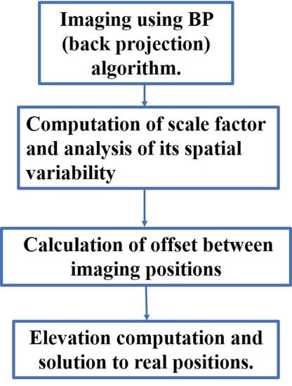
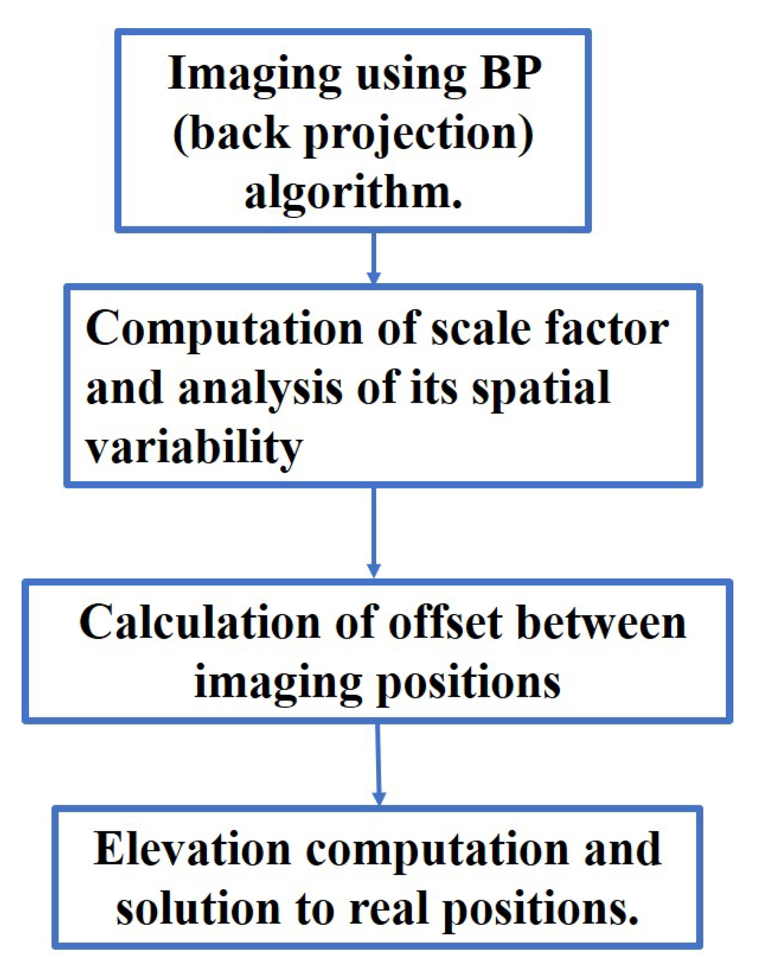
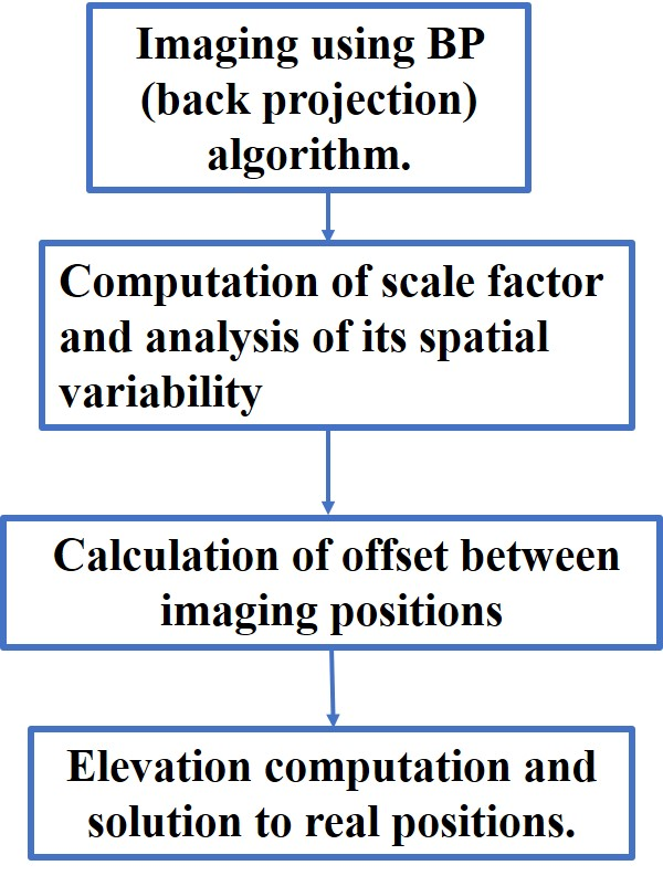
k given above, this section presents an approach for DEM generation with scale factor using offset of imaging positions in multi-aspect images. Then the procedure of DEM generation method is described in detail for multi-aspect images, which is shown in
Figure 3. BP algorithms [
22] stated in Step 1 will not be introduced in this paper. The subsequent parts focus on the Step 2 to Step 4.
Step 1: Each image is formed directly in ground coordinate by back projection (BP) algorithm.
Step 2: According to the velocity vector and position vector of the SAR platform at the instantaneous position, determine the imaging position of the target. Calculate the equivalent incidence angle and equivalent aspect angle. Figure out the scale factor k in the current scene. To simplify the process of computation for scale factor k, spatial variability of it needs to be analysed based on the real data for application.
Step 3: Normalized cross correlation (NCC) is conducted on two aspect images to obtain offset between imaging positions.
Step 4: Based on (
7), absolute value of height difference
is obtained and real positions that is three dimensional coordinate of targets can be solved.
If N groups of different aspect angle images are used, offset with maximum of correlation coefficient is considered to be a more correct value. N height maps were combined to get a final complete DEM.
3.1. Calculation of the Scale Factor
As is shown in (
8), scale factor
k is related with the equivalent incidence angle and the difference between the equivalent aspect angle. The coordinate
of the imaging position when the target is observed from a certain aspect angle can be obtained by Range-Doppler principle.
3.1.1. Calculation of Equivalent Incidence Angle
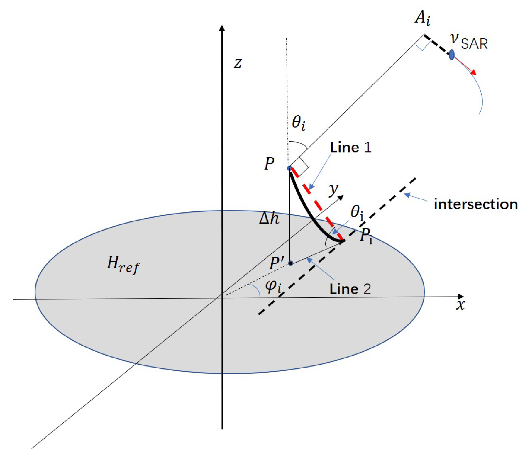
According to the geometric relationship shown in
Figure 4, the equivalent incidence angle
corresponding to a viewing aspect angle can be obtained by (
9).
3.1.2. Calculation of Difference Equivalent Aspect Angle
According to (
8),it is not necessary to solve the specific values of equivalent angles
and
. Only difference of two aspect angles is needed.
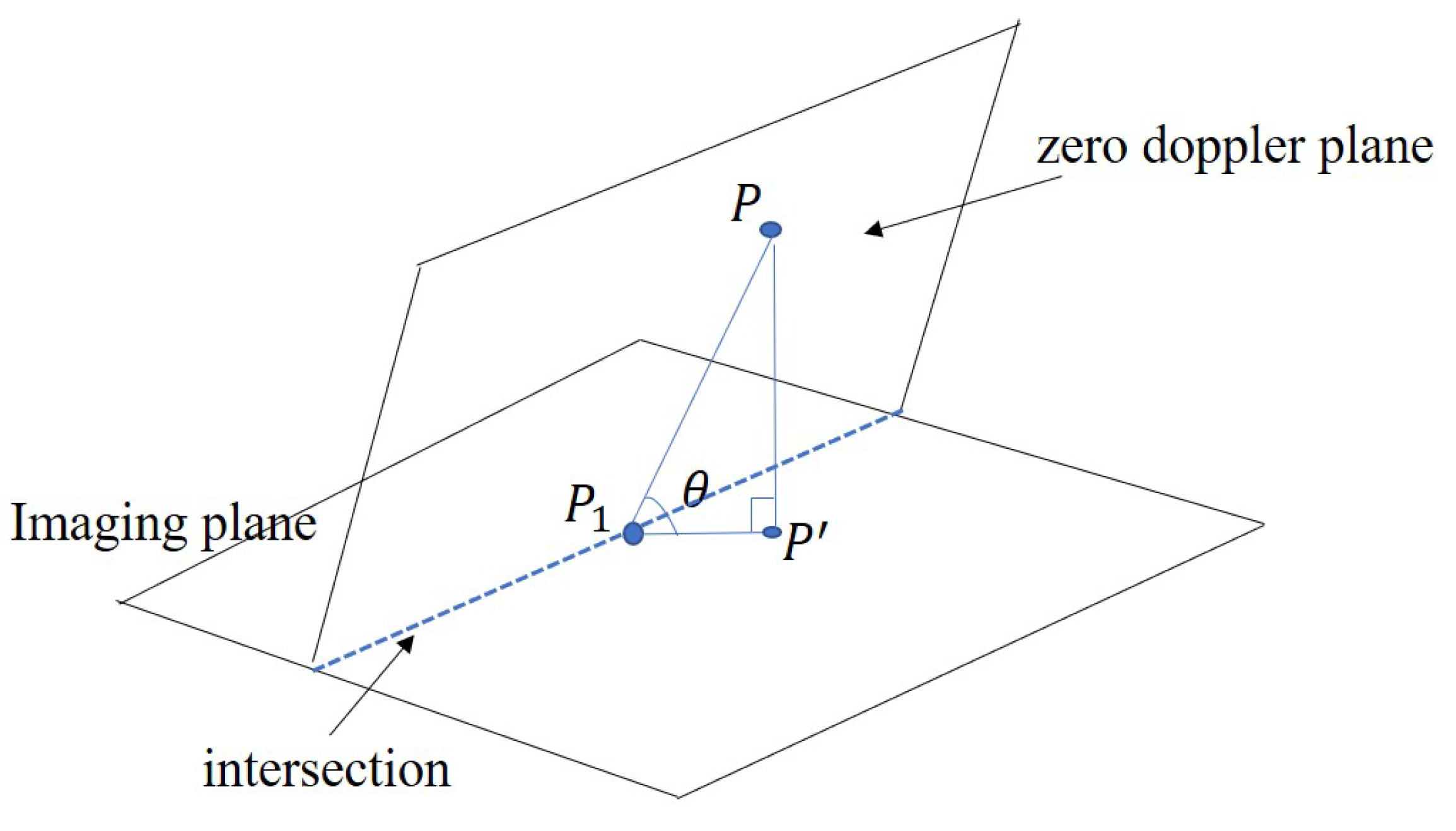
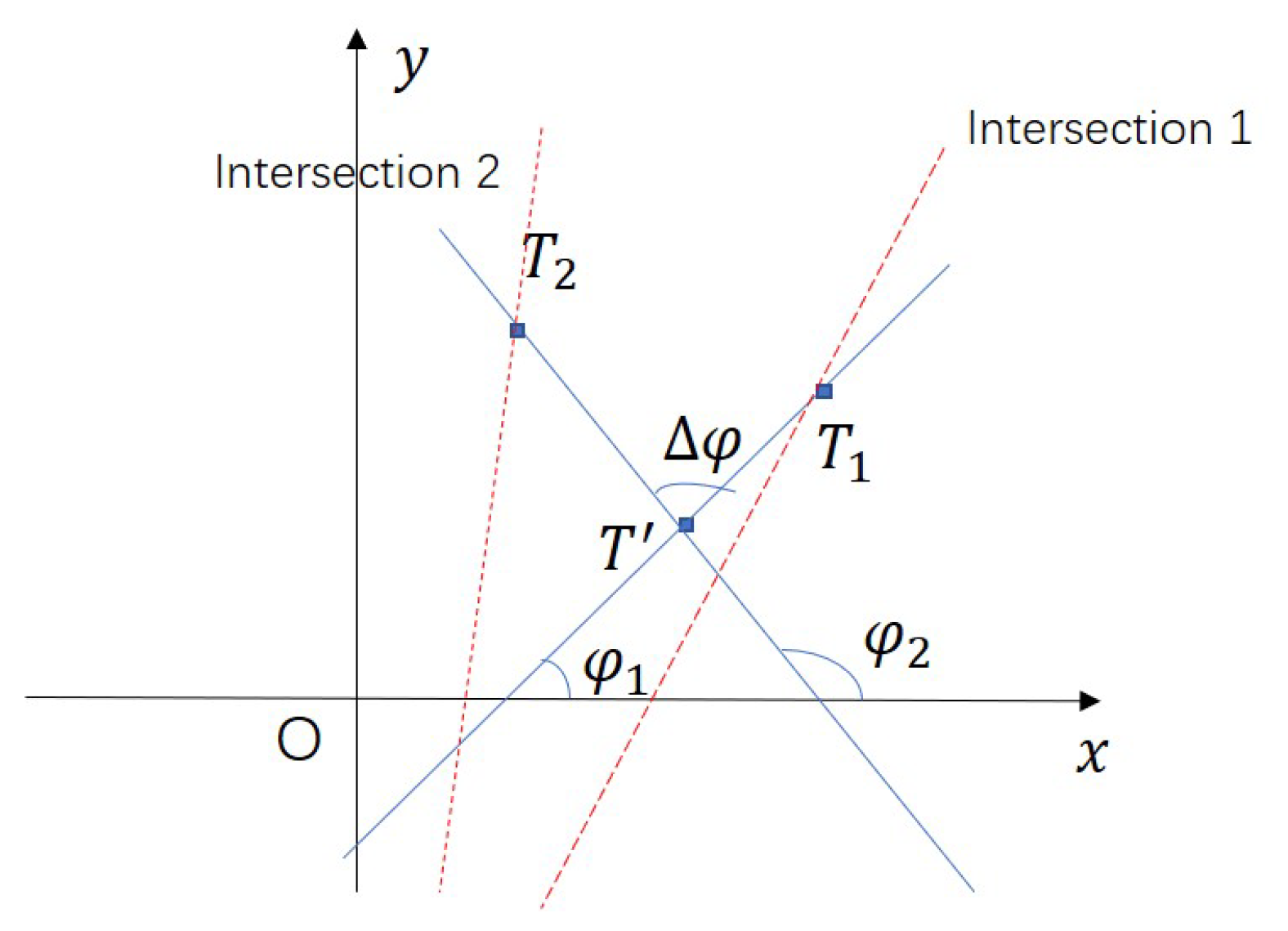
Figure 5 is the top view of the reference imaging plane.
,
are the imaging positions from two viewing aspect angles which are obtained by the Range-Doppler imaging model.
and
are equivalent angles under two viewing aspect angles respectively. The intersection refers to the intersection of zero Doppler plane and scene plane under one certain viewing aspect angle. Let
.
As is shown in
Figure 5, (
11) can be obtained by the law of cosines.
Therefore, difference of two aspect angles
can be solved by (
12).
To simplify the process of computation for scale factor k, spatial variability of it needs to be analysed based on the real data for application. From engineering point of view, point targets are set in the ground coordinates in accordance with the coordinate system used in imaging process.Under any two viewing aspect angles, we computed scale factor k point by point. The precise scale factor k of each point target is obtained. Finally, we compare all of scale factors k of target points at different positions with the k obtained at the center of the scene. Then the variation of proportional coefficient in the given scene area is analysed.
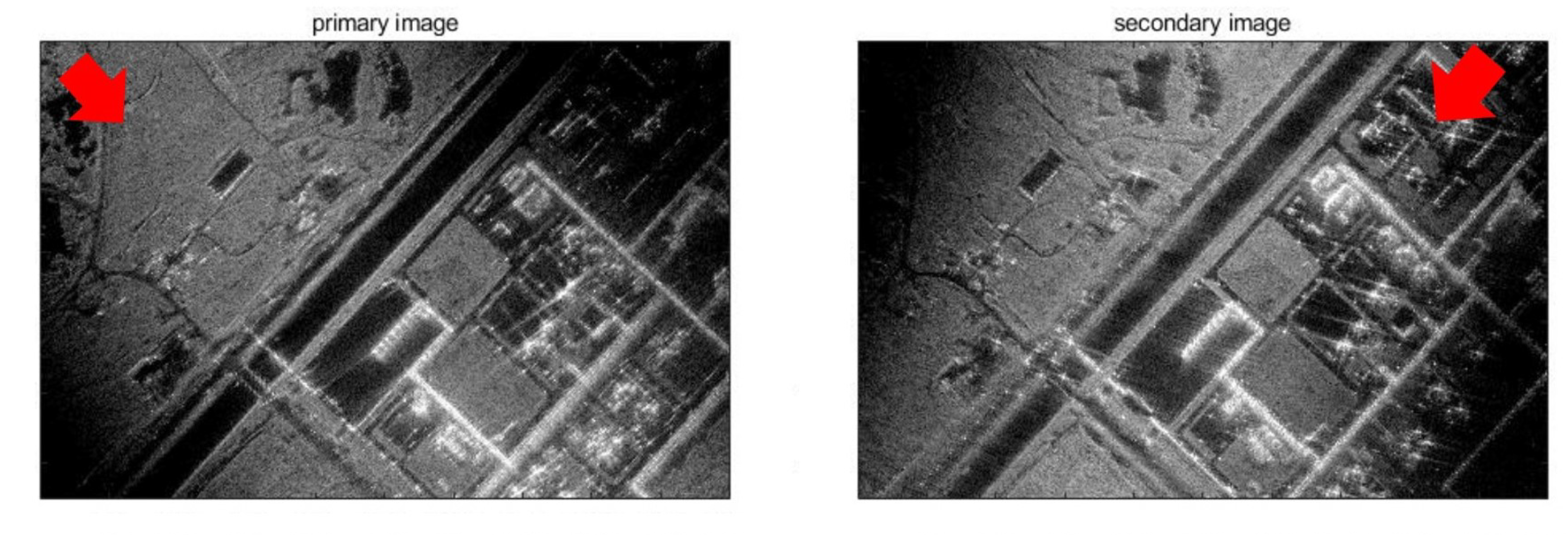
3.2. Calculation of Offset between the Imaging Positions in Different Aspect Images
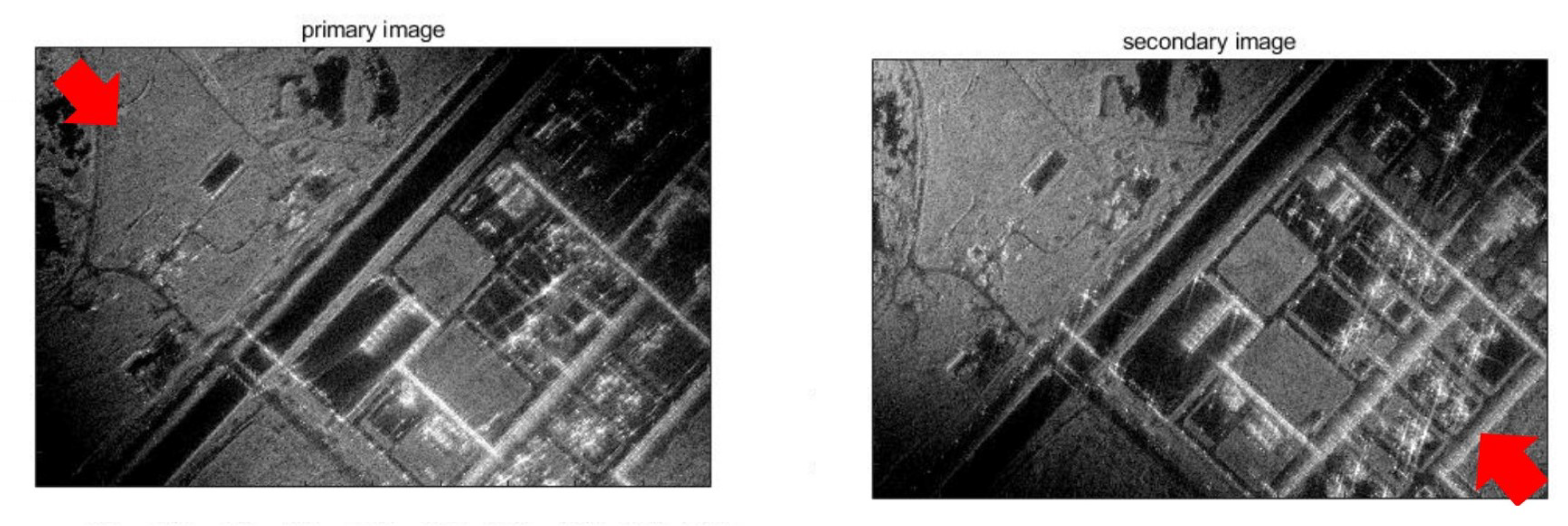
In this part, image registration is conducted to find homogeneous points in multi-aspect images and offset is calculated. NCC [
23] is applied to obtain the best matching patches.
is the center of any sub-area in a primary image. The template window traverses on the searching area in the secondary image and normalized cross-correlation coefficient
of each corresponding area to the template window is calculated by (
13).
where,
and
are intensity of template window in primary image and secondary image respectively.
and
are mean of the corresponding areas.
The pixel corresponding to the maximum correlation coefficient in secondary image is matching area and the offset of the corresponding areas is
where,
and
are actual size of imaging grid.
Afterwards, supposing that the homogeneous points obtained by image registration are precise, offset between the two points is exactly accurate. However, target can only be illuminated in certain aspects.So we can use multiple pairs of aspect images to obtain the homogeneous points. For each ground cell of imaging grid, the patches with maximum of correlation coefficient are considered to be more correct.
3.3. Elevation Computation and Solution to Three-Dimensional Coordinates
Offset is converted to absolute value of height difference easily by the elevation extraction model proposed in
Section 2.2.
Three-dimensional coordinates needs to be solved for reconstruction. can be negative or positive depending on whether the target is above or below the imaging plane. First, discrimination method of is shown. Then Z coordinate of target can be obtained. Two-dimensional coordinates are solved by a system of equations. Two sets of solutions will be obtained, and the correct group of solutions is selected by relative relationship between the target and the imaging plane.
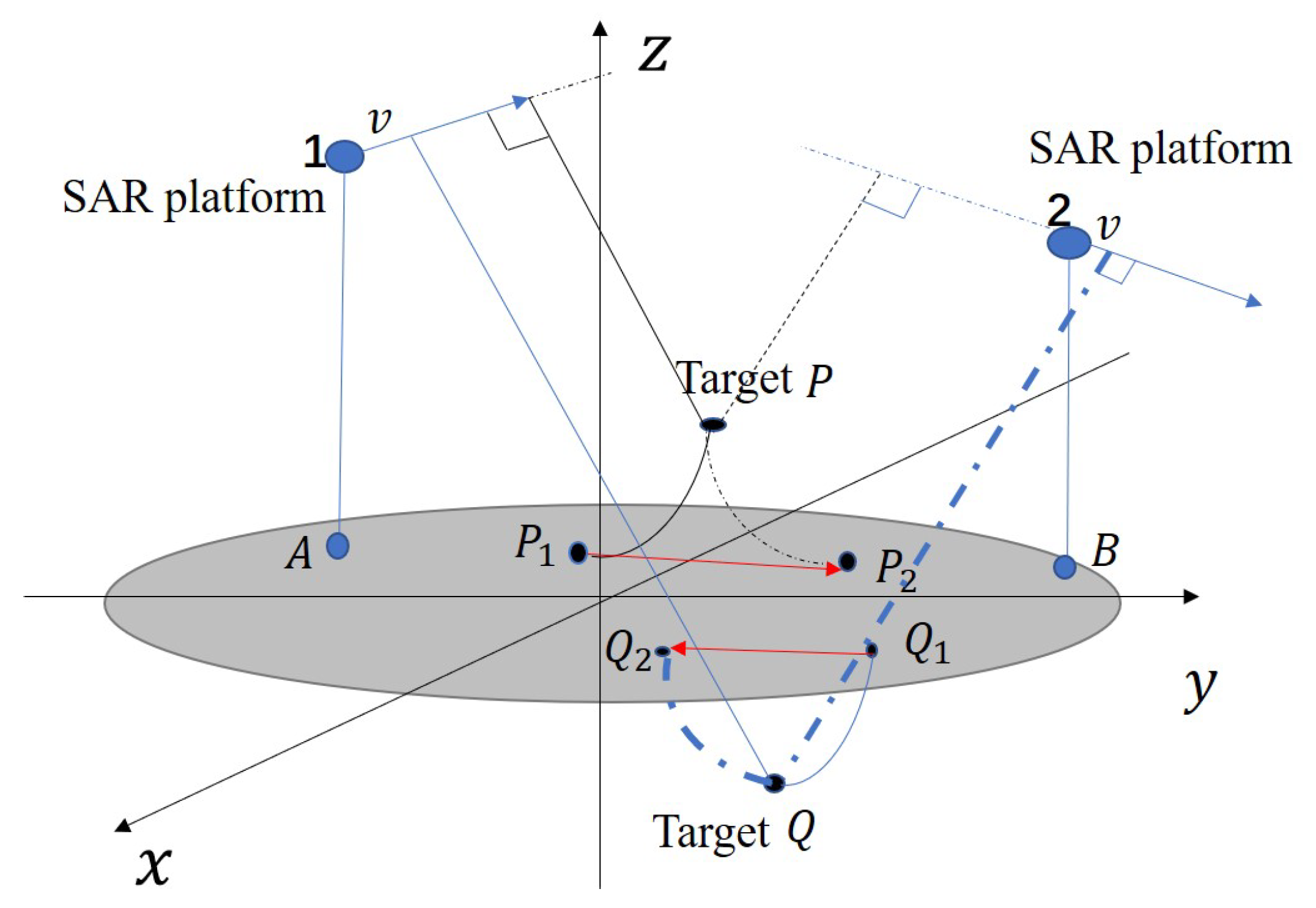
3.3.1. Determination of Z Coordinate
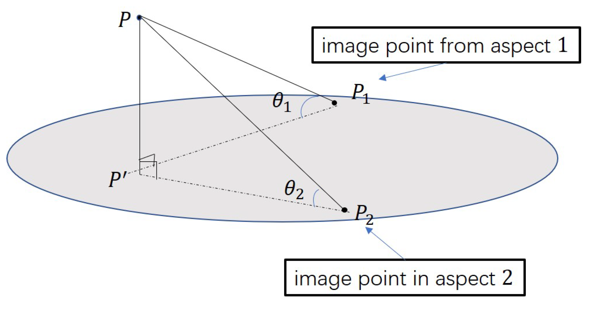
Supposing that at two viewing aspect angles 1 or 2, the plain coordinates of SAR platform are and respectively. The target that is above or below the imaging plane will be projected to different positions. Therefore, the angle between the SAR platform position vector and the imaging positions vector can be used to determine whether the target is above or below the imaging plane.
As shown in
Figure 6, when target
is above imaging plane
.
and
are imaging positions when the plain coordinates of SAR are
A and
B respectively. It can be easily obtained that
For target
below the imaging plane, which means
,
and
are imaging positions from two viewing aspect angles. Additionally,
is the imaging position when SAR is at position 1.
Therefore, when imaging positions vector and radar positions vector satisfy with (
15), which means the angle between two vectors is less than
, target is above the imaging plane. The
Z coordinate of target is
.
When imaging positions vector and radar position vector satisfy with Equation (
16), which means the angle between two vectors is more than
, target is below the imaging plane. The
Z coordinate of target is
.
3.3.2. Solution to Planimetric Coordinates
After
Z coordinate of the target is derived, we need to solve the planimetric coordinates of the target:
X coordinate and
Y coordinate to get the complete three-dimensional coordinates. Assuming that the true three-dimensional coordinates of the target is
. According to the analysis in
Section 2.2, geometric relationship of target, imaging positions and projections from two viewing aspect angles is shown in
Figure 7.
Equations for
,
are
where
,
are the plane coordinates of imaging positions obtained from two viewing aspect angle 1 and 2 respectively. Two groups of solutions will be obtained from the above equations.
The method for determining the correct group of solution is stated as follows:
Shown in
Figure 6, if the target
P is above the imaging plane whose
Z coordinate is
, the correct group of solution
satisfies (
18):
If the target
Q is below the imaging plane whose
Z coordinate is
, the correct solution
satisfies (
19):
4. Experimental Result
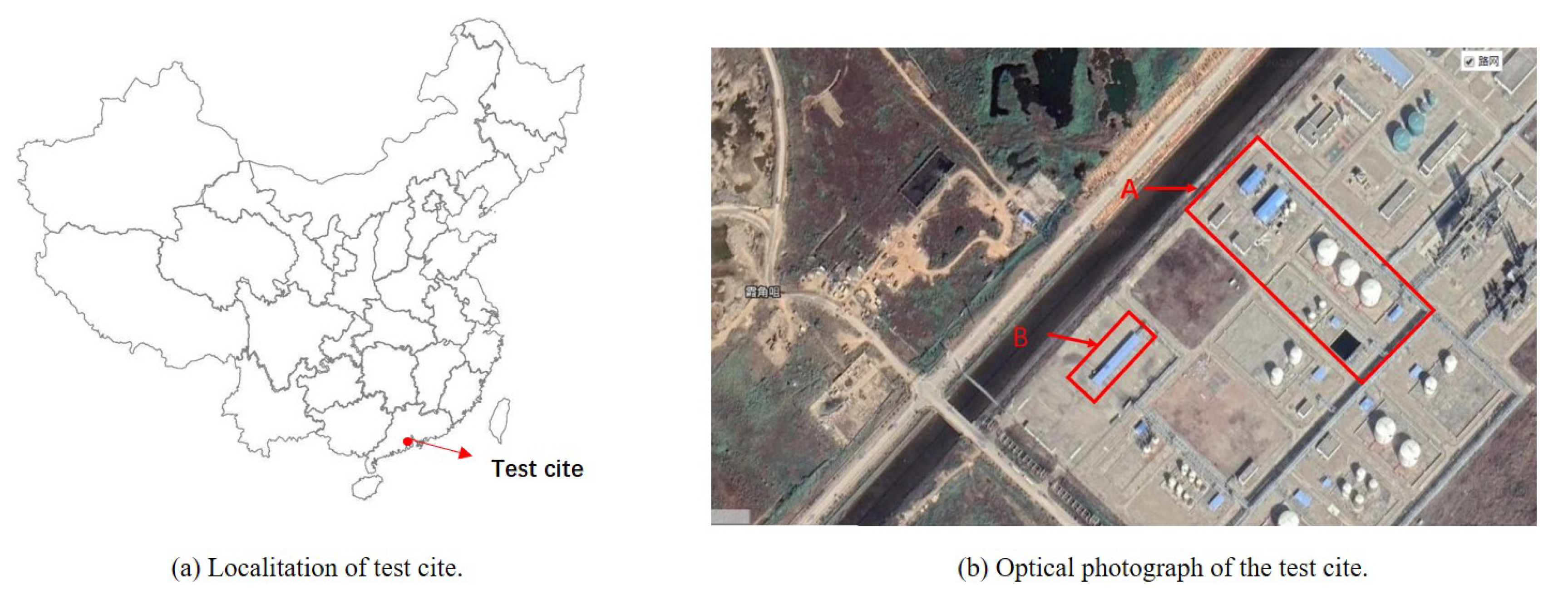
In this section, we experiment on C-band airborne CSAR data (see
Table 1 for acquisition characteristics). The dataset is acquired over a test site in located in Zhuhai, a coastal city in Guangdong province of southern China, as shown in
Figure 8a. Optical photograph of the scene is shown in
Figure 8b. The circular flight experiment was conducted by the Aerospace Information Research Institute, Chinese Academy of Sciences. The terrain in this area is relatively flat. CSAR is capable of providing multi-aspect images which is called sub-aperture images [
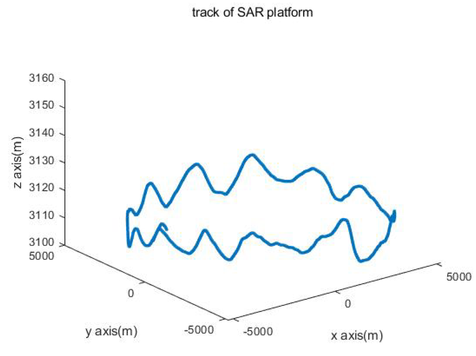
24]. Different sub-aperture images are formed in one ground coordinate system. The track of SAR platform is shown in
Figure 9, which realizing multi-aspect observation. Velocity vector changes both in yaw direction and pitch direction. The following experiments were conducted with the MATLAB R2018a software on a computer with an Intel Core 3.2-GHz processor and 8.0 GB of physical memory.
BP algorithm [
22] is used to form sub-aperture image in the ground coordinates. The reference imaging height plane is set to 20 m. The pixel spacing is set to 0.5 m. In this experiment, two pairs of sub-aperture images are chosen. Each sub-aperture image covers 6
via magnitude accumulation, which is shown in
Figure 10 and
Figure 11. It is obvious that the direction of illumination is different at each viewing aspect angle.
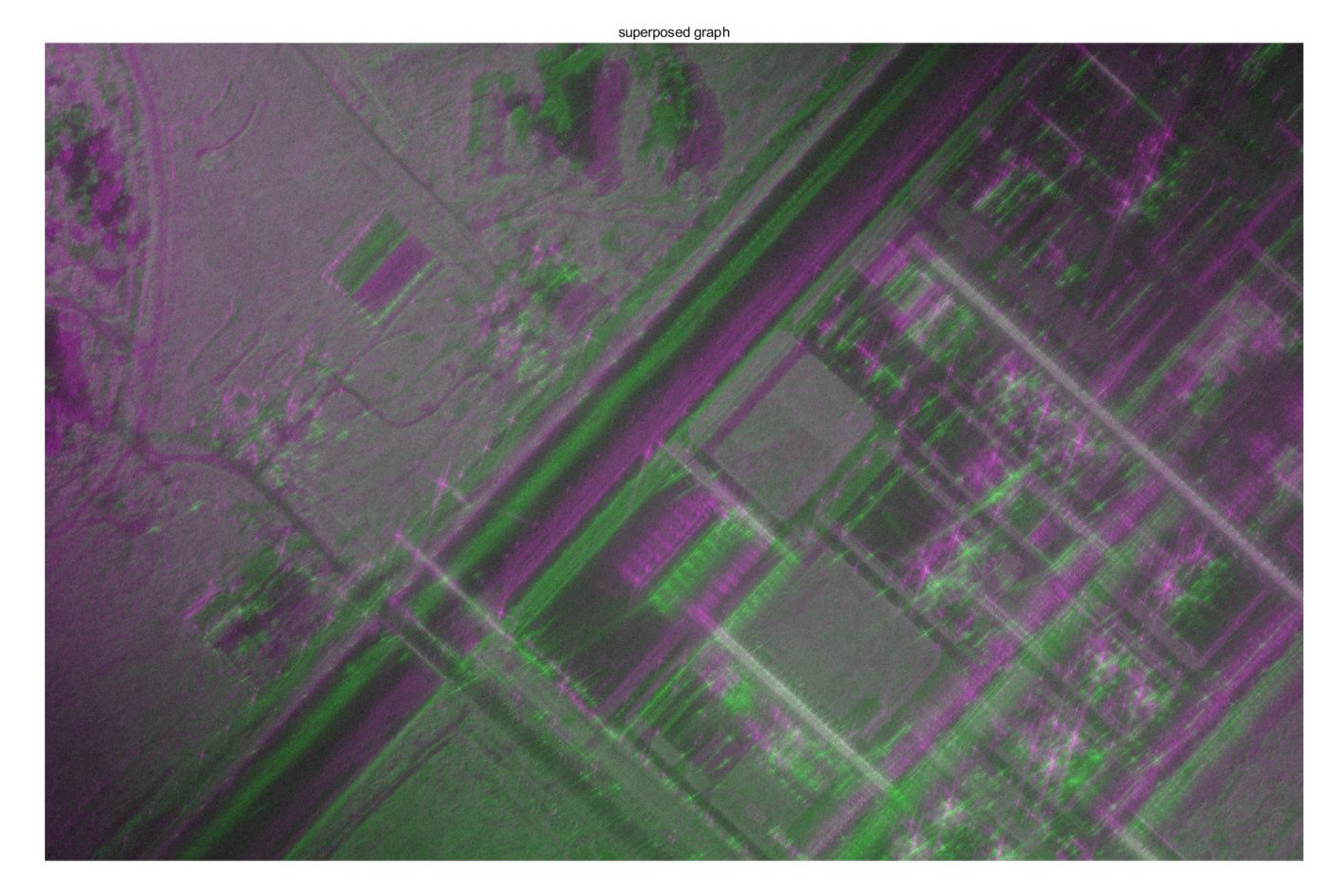
SAR images from two viewing aspect angles which are labelled by different colors are shown in
Figure 12. Purple color and green color denote two images acquired at two different viewing aspect angles. It can be seen that offset of two images is obvious. The main difference in the two-aspect images is translation indicating that the terrain is relatively flat.
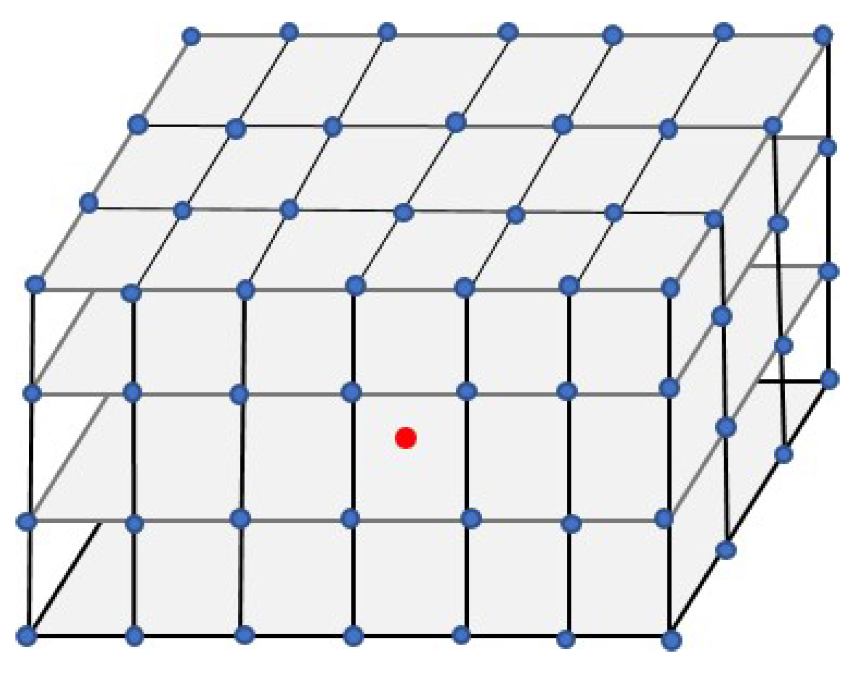
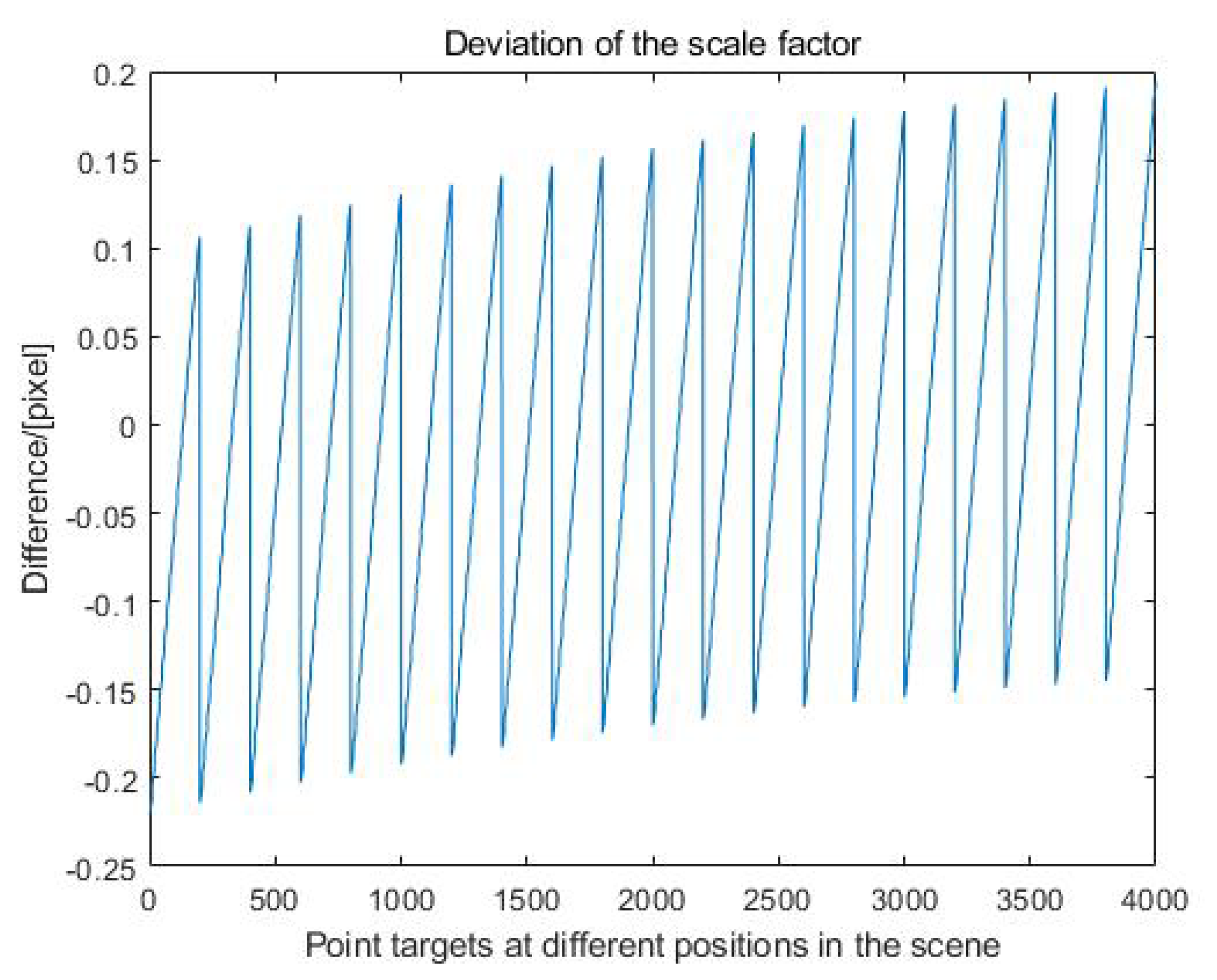
To simplify the process of computation for scale factor
k, spatial variability of it will be analysed based on the C-band airborne CSAR data in the experiment. From an engineering point of view, point targets (each target is set at every 50 m in the plane range and every 5 m in the height range) with a coverage area of 1 km in length and 50 m in height is set in the ground coordinates in accordance with the coordinate system used in BP imaging process, shown in
Figure 13. Under any two viewing aspect angles, we computed scale factor
k point by point according to (
8). The precise scale factor
k of each point target is obtained. Finally, all of scale factors
k of target points at different positions are compared with the
k obtained at the center of the scene. Then we calculate the deviation value between them.
Deviation of scale factor
k between any points and the target
at scene center is shown in
Figure 14. Deviation is between −0.2 and 0.2.
According to (
7), height sensitivity versus pixel offset between the images can be deduced by (
20)
where
is the offset of imaging positions in ground coordinates between two viewing aspect angles. As is defined before, scale factor
k is related with equivalent incidence angle and difference of equivalent aspect angles. These two angles depend on different positions in the scene, which introduces spatial varying scale factors.
Therefore theoretical precision of height estimation depends on precision of offset and scale factor k. Pixel size in this experiment is 0.5 m. The scale factor k for the first pair of sub-aperture images is 2.0012. Corresponding to one-pixel accuracy in matching process, height error caused by mismatching is 1.0006 m, while height error caused by deviation of k is −0.2001 m to 0.2001 m. Scale factor k for the second pair is 0.76968. Corresponding to one-pixel accuracy in matching process, height error caused by mismatching is 0.3848 m, while height error caused by deviation of k is −0.077 m to 0.077 m.
As above analysis, though the scale factor k varies from place to place within the set range, the error caused by scale factor k is not obvious compared with the error caused by matching process. In this experiment we only need to calculate the scale factor in the scene center instead of point by point. Therefore scale factor k of target at scene center is chosen to be a global value.
NCC algorithm is conducted to get offset between imaging positions in each pair of images. In this experiment, the value of normalized correlation coefficient threshold is 0.3. Offset between the imaging positions can be calculated. Then offset is converted to absolute value of height difference easily by the elevation extraction model proposed in
Section 2.2.
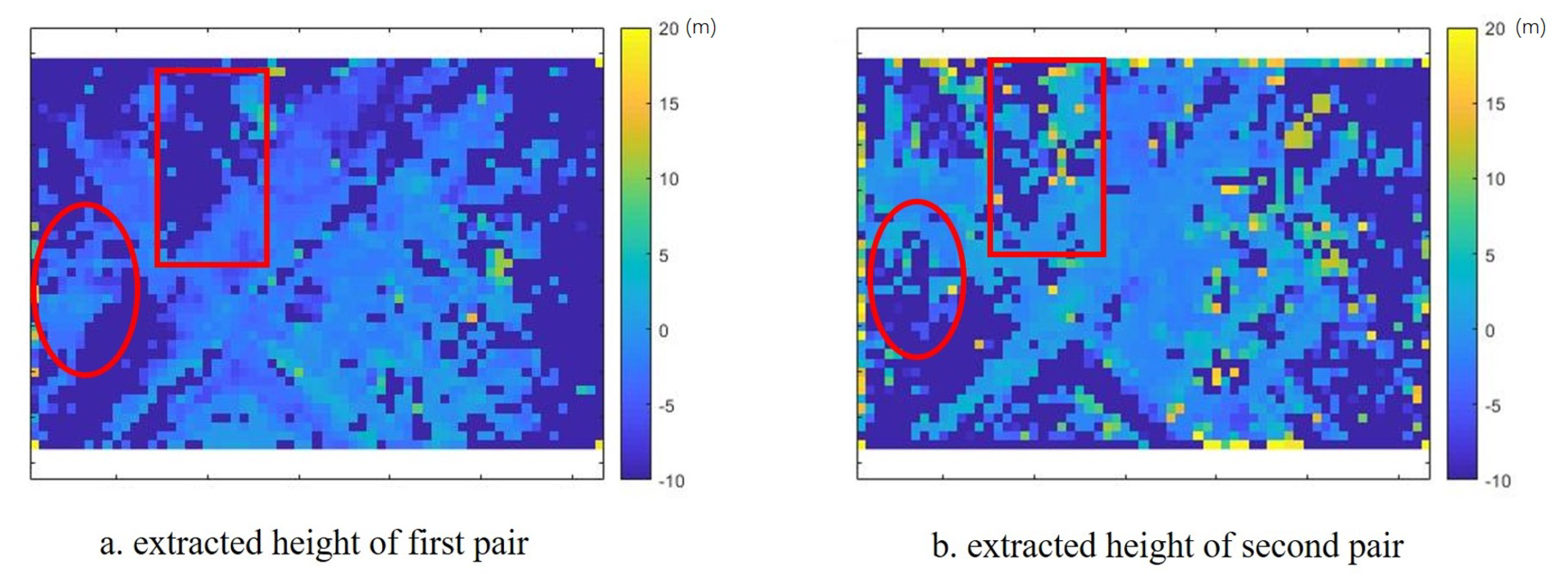
The preliminary elevation map of the scene generated by each pair of sub-aperture image is shown in
Figure 15a,b. The areas which have been matched well can obtain relatively accurate results. Dark blue areas are unknown altitudes which are set to −10 m. When imaging at each viewing aspect angle, the range of radar beam coverage is different. Some areas are not illuminated in the first group of images but are illuminated in the second group of images. Therefore, the height information of such area obtained from the second group of images is relatively accurate. Therefore the height information obtained from two groups of aspect images provides a relatively complete height map. For example, for the area in an elliptic region, the result is better in
Figure 15a than in
Figure 15b. While for area in rectangular region, height information obtained in
Figure 15b is better than in (a).
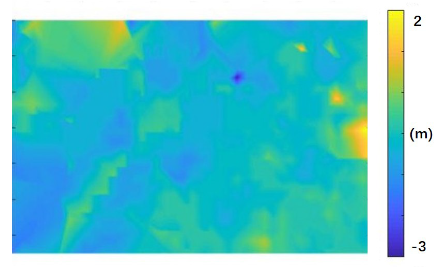
Take advantage of different viewing aspect angles, elevation with a larger correlation coefficient will be assigned to the target. Therefore, final elevation value will be obtained by considering two pairs of aspect angles information. Finally, we can get a final DEM after interpolation, shown in
Figure 16. The terrain in this scene is between −3 m and 2 m.
The effectiveness of extracted DEM is evaluated in two ways. The first is to compared with the elevation value with TanDEM-X 90 m DEM provided by German Aerospace Center (DLR) [
https://tandemx-90m.dlr.de/, in 2016]. Here is a brief quantitative analysis of the estimated errors compared with the height information. Mean value and root mean square error (RMSE) are used to quantitatively evaluate the estimation accuracy, shown in
Table 2. RMSE can be calculated by
where
N denotes the number of all the pixels in the SAR image.
is the height information provided by DLR.
is the height information obtained by proposed method.
Shown in
Table 2, average height of this scene obtained by the proposed method is −0.4688 m. Mean value of the scene calculated by TanDEM-X 90m DEM is −1.6961 m. The RMSE of the heights obtained by our method is 2.0036 m.
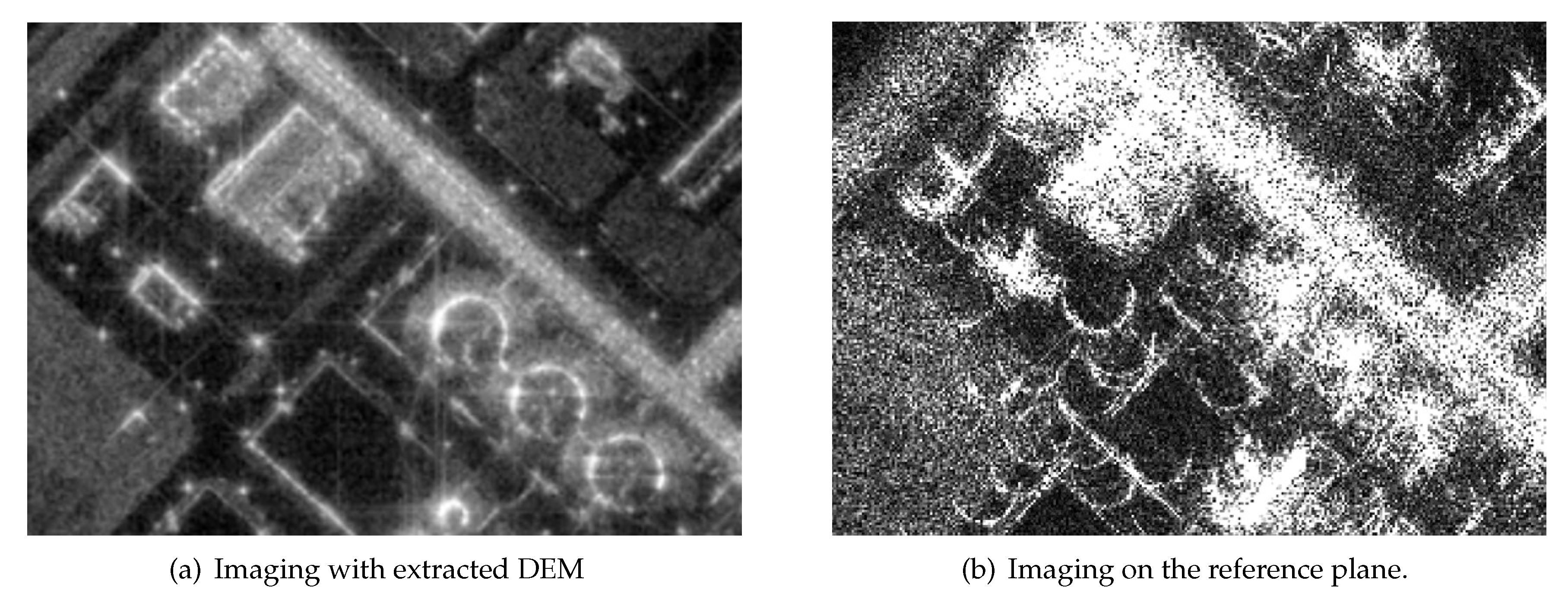
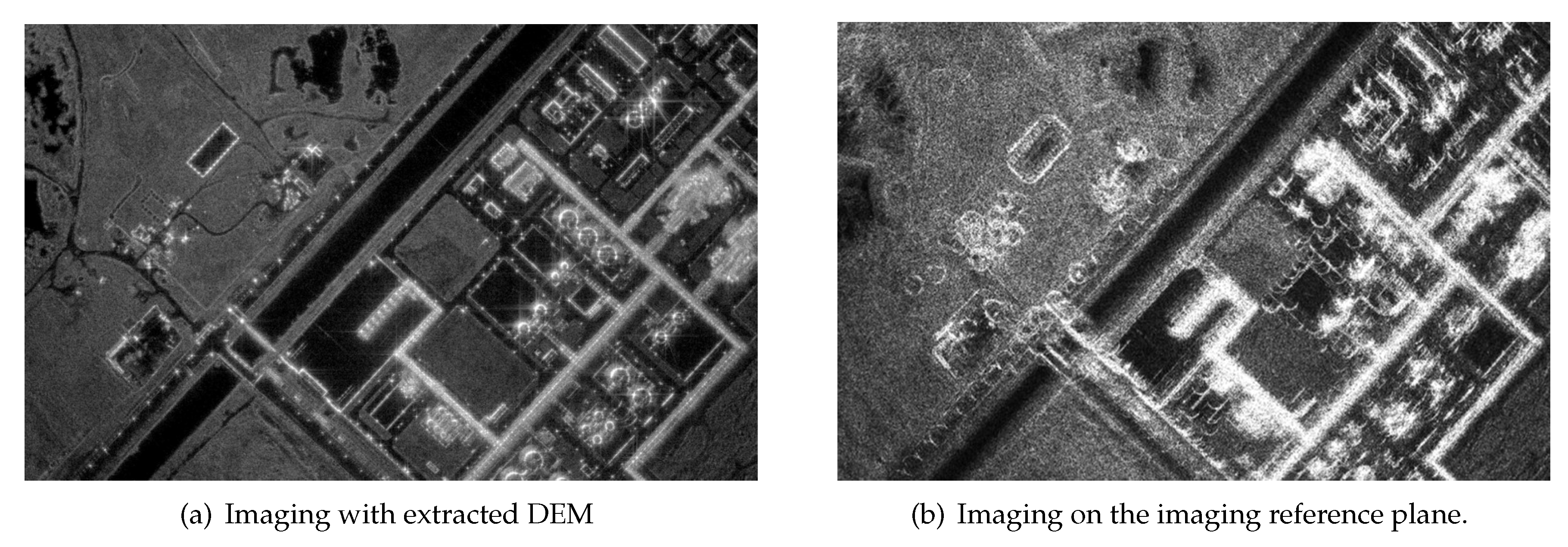
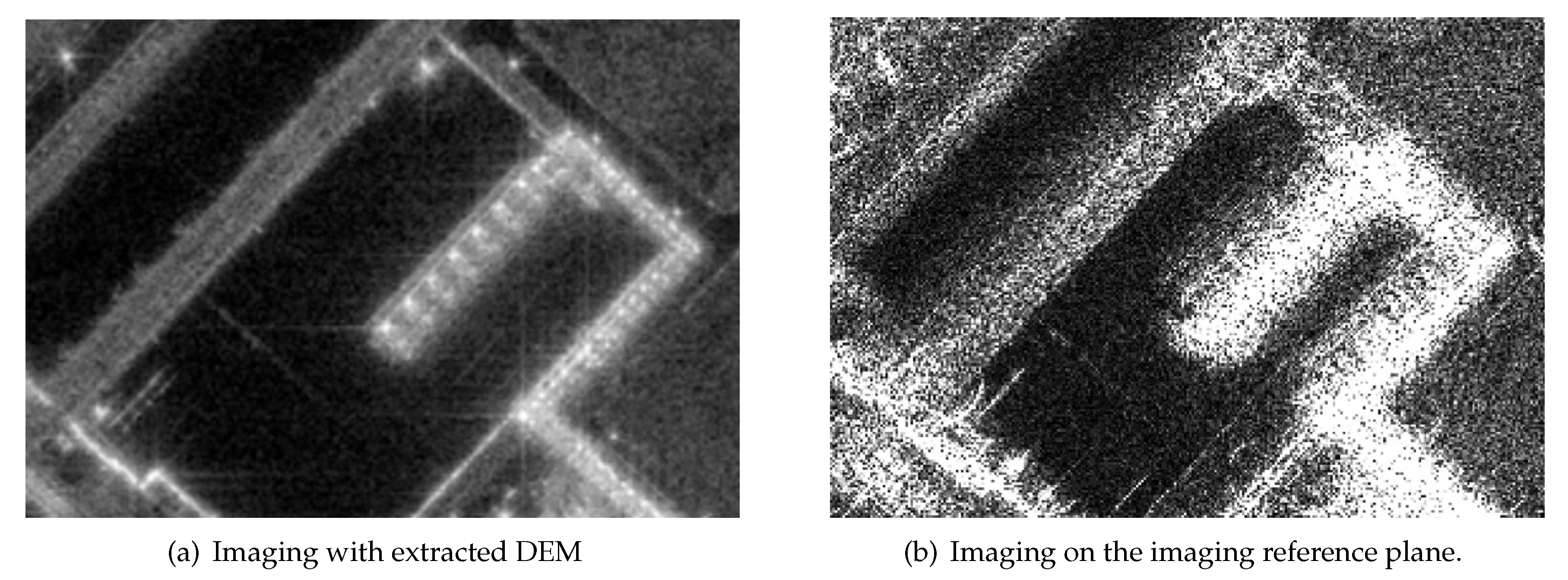
The second way is to reimage the CSAR data using BP algorithm with extracted DEM. The image formed via magnitude accumulation of all the sub-aperture images is shown in
Figure 17a. Compared with the image whose imaging reference plane is 20 m (
Figure 17b), defocusing has been obviously improved. The imaging position in different sub-aperture images is projected to the right position. Therefore the extracted DEM helps to improve the quality of all-aperture image, which is validated the effectiveness.
Then we show some details. As shown in
Figure 8, there are some buildings in region A and region B. In
Figure 18b and
Figure 19b, the defocusing phenomenon is so serious that it is impossible to distinguish what object it is.
5. Discussion
The method proposed in this paper is mainly aimed at the new multi-aspect imaging mode which is beneficial for finer observation. The common way is to establish the stereoscopic image pair by using the SAR images formed on slant plane or ground plane and then location of target is obtained by solving the the RD equations.
Actually, when images formed on the ground plane, the imaging coordinate system is unified. From the perspective of imaging, the target, which is above or below the imaging plane, will be projected to different positions from different aspect angles, shown in
Figure 17b, and when height of target is equal to the imaging plane, it will be projected to the right position whichever the aspect angle is, shown in
Figure 17a. We deduced that the offset between imaging positions is proportional to the height difference and obtained the scale factor to describe the linear relationship.
So for multi-aspect images such as CSAR images and wide-angular spot images, which are always generated on the ground plane, there is no need to solve the Range-Doppler equations point by point. We can retrieve the height value directly when the offset between imaging positions is acquired. If it is a lawn with similar terrain height, the offset of this area is roughly the same. Therefore only the overall offset needs to be solved instead of solving the location of targets point by point. Thus it is more efficient for multi-aspect imaging mode.
When DEM map is applied in imaging process, imaging positions from different aspect angles of the target will be projected to the same position, and thus the high quality wide-angular aperture image will be obtained after several different aspect images are incoherently superimposed, shown in
Figure 18a and
Figure 19a.
Since the scale factor is determined by the velocity vector and position vector of SAR at instantaneous time, the proposed method can be used to retrieve the elevation of any given two SAR images with high accuracy. In this experiment, the scale factor at the scene center is chosen to be a global value. From the analysis of variation for the scale factor in the scene, shown in
Figure 14, we found that the error caused by the scale factor can be neglected. If the scene is rather large, the scale factor can by solved in several small regions.
The proposed method could be applied in urban spaces where studied objects have to be observed from different point of views. Special phenomena of the shadow region, overlays or reflectors in the high-resolution SAR images bring difficulties to SAR imagery understanding due to synthetic aperture [
25]. Urbanized spaces are particularly characterized by those affects. Therefore, omni-directional observation and image sequence processing can be taken into consideration [
26]. DEM generated by our method is suitable for multi-aspect imaging mode and can greatly improve the results of multi-aspect imaging. In this way, high-quality multi-aspect images can help a lot for urban SAR imagery understanding [
27].
However, due to characteristics of urban environments, registration of images is difficult. Especially for the SAR images acquired at different aspects, backscattering characteristics of the same object at different aspects vary greatly [
28], which makes it easy to be recognized as different objects in multi-aspect images. Meanwhile, intensity of multi-aspect images can also change a lot. Besides, there are so many corner reflectors in urban areas, which is extremely sensitive to different viewing aspects. That makes images over urban areas especially difficult to match [
29]. Further investigation has reminded a challenging task.

 ,
, 


