Article

Vertical Wind Shear Modulates Particulate Matter Pollutions: A Perspective from Radar Wind Profiler Observations in Beijing, China

1
State Key Laboratory of Severe Weather, Chinese Academy of Meteorological Sciences, Beijing 100081, China
2
School of Atmospheric Physics, Nanjing University of Information Science and Technology, Nanjing, 210044, China
3
Institute of Environment, Energy and Sustainability, The Chinese University of Hong Kong, Shatin, New Territories, Hong Kong 999077, China
4
School of Earth and Space Sciences, University of Science and Technology of China, Hefei 230026, China
5
Department of Geography and Resource Management, The Chinese University of Hong Kong, Shatin, New Territories, Hong Kong 999077, China
6
Stanley Ho Big Data Decision Analytics Research Centre, The Chinese University of Hong Kong, Shatin, New Territories, Hong Kong 999077, China
*
Author to whom correspondence should be addressed.
Remote Sens. 2020, 12(3), 546; https://doi.org/10.3390/rs12030546
Submission received: 6 January 2020 / Revised: 2 February 2020 / Accepted: 4 February 2020 / Published: 7 February 2020

Abstract

:
Vertical wind shear (VWS) is one of the key meteorological factors in modulating ground-level particulate matter with an aerodynamic diameter of 2.5 µm or less (PM2.5). Due to the lack of high-resolution vertical wind measurements, how the VWS affects ground-level PM2.5 remains highly debated. Here we employed the wind profiling observations from the fine-time-resolution radar wind profiler (RWP), together with hourly ground-level PM2.5 measurements, to explore the wind features in the planetary boundary layer (PBL) and their association with aerosols in Beijing for the period from December 1, 2018, to February 28, 2019. Overall, southerly wind anomalies almost dominated throughout the whole PBL or even beyond the PBL under polluted conditions during the course of a day, as totally opposed to the northerly wind anomalies in the PBL under clean conditions. Besides, the ground-level PM2.5 pollution exhibited a strong dependence on the VWS. A much weaker VWS was observed in the lower part of the PBL under polluted conditions, compared with that under clean conditions, which could be due to the strong ground-level PM2.5 accumulation induced by weak vertical mixing in the PBL. Notably, weak northbound transboundary PM2.5 pollution mainly appeared within the PBL, where relatively small VWS dominated. Above the PBL, strong northerlies winds also favored the long-range transport of aerosols, which in turn deteriorated the air quality in Beijing as well. This was well corroborated by the synoptic-scale circulation and backward trajectory analysis. Therefore, we argued here that not only the wind speed in the vertical but the VWS were important for the investigation of aerosol pollution formation mechanism in Beijing. Also, our findings offer wider insights into the role of VWS from RWP in modulating the variation of PM2.5, which deserves explicit consideration in the forecast of air quality in the future.

Graphical Abstract

1. Introduction

Particulate particle with an aerodynamic diameter of 2.5 μm or less (PM2.5), mainly originated from industrial emissions and vehicle exhaust pollutants, and secondary aerosols forming through a series of photochemical reactions [1,2] have been shown to significantly affect the atmospheric environment [3,4,5], weather and climate system [6,7,8,9,10,11,12,13,14,15], and human health [16,17,18,19]. Therefore, the PM2.5 pollution and its causes have been increasingly receiving attention in recent years [20,21].
The major drivers for deteriorating or improving PM2.5 pollution are roughly twofold—aerosol emissions and meteorology—both of which are highly versatile and uncertain. In addition to high emissions accompanied with the rapid development of urbanization and industrialization, the roles of meteorological conditions, including large-scale synoptic patterns [22,23,24,25,26], and local meteorological conditions in the planetary boundary layer (PBL) [27,28,29,30,31,32] have been well recognized able to modulate the PM2.5 concentration. For instance, Tai et al. [27] revealed that the local meteorological conditions could explain up to 50% of the daily variability of PM2.5 in the USA from 1998 to 2008. In 68 major cities of China, ground-level PM2.5 were found to be broadly associated with local meteorological factors at seasonal, yearly, and regional scales [33]. Among various meteorological factors, the surface wind speed was one of the variables modulating ground-level PM2.5 over the Yangtze River Delta region of China, which showed that PM2.5 decreased approximately by -2.42 µg m−3 for a 1 m s−1 increase in wind speed [34]. In Beijing, the heavy pollution events frequently occurred under the calm wind conditions, which was generally associated with stable atmospheric stratification and shallow PBL [35,36,37,38]. The presence of high pressure in northwest parts of Beijing, linked to strong northwesterly winds, was closely associated with a significant drop in PM2.5 concentrations in Beijing [4]. Besides, the changes in circulation induced by local mountain-valley and urban heat island setting in Beijing and its surrounding areas were found to be able to modulate the diurnal variations of PM2.5 in Beijing [32].
Among others, reanalysis data and model simulations were one of the most used approaches to analyze the variation of wind with different height in the lower troposphere and its impacts on air pollution, revealing a significant role of vertical wind shear (VWS, an important indicator of dynamically vertical mixing) in modulating particulate matter pollution [37,39,40]. In recent years, there has been a surge of interest in observational investigation of VWS in connection with atmospheric pollution, most of which are based on Doppler wind lidar [26,39]. However, the Doppler wind lidar has limited capability to offer vertically resolved wind observations under pretty clean or foggy conditions. To date, the associations between vertical wind profile and surface particulate matter concentrations have yet to be fully understood in Beijing.
Fortunately, the new-generation radar wind profiler (RWP) deployed by the China Meteorological Administration (CMA) in Beijing [41] offers us the best opportunity to quantify the long-term effect of local wind vector profiles and VWS on ground-level PM2.5 pollution in Beijing. Thus, this study aims to explore the impacts of wind profiles and VWS on the wintertime PM2.5 in Beijing based on high-resolution RWP observation along with ground-level PM2.5 monitoring. The remaining contents of this work proceed as follows. In Section 2, the measurements of RWP, other related weather data, and ground-level PM2.5 are described in detail. In Section 3, the impacts of wind and VWS on PM2.5 pollution in Beijing are analyzed and discussed. Finally, the main findings are summarized in Section 4.

2. Data and Methodology
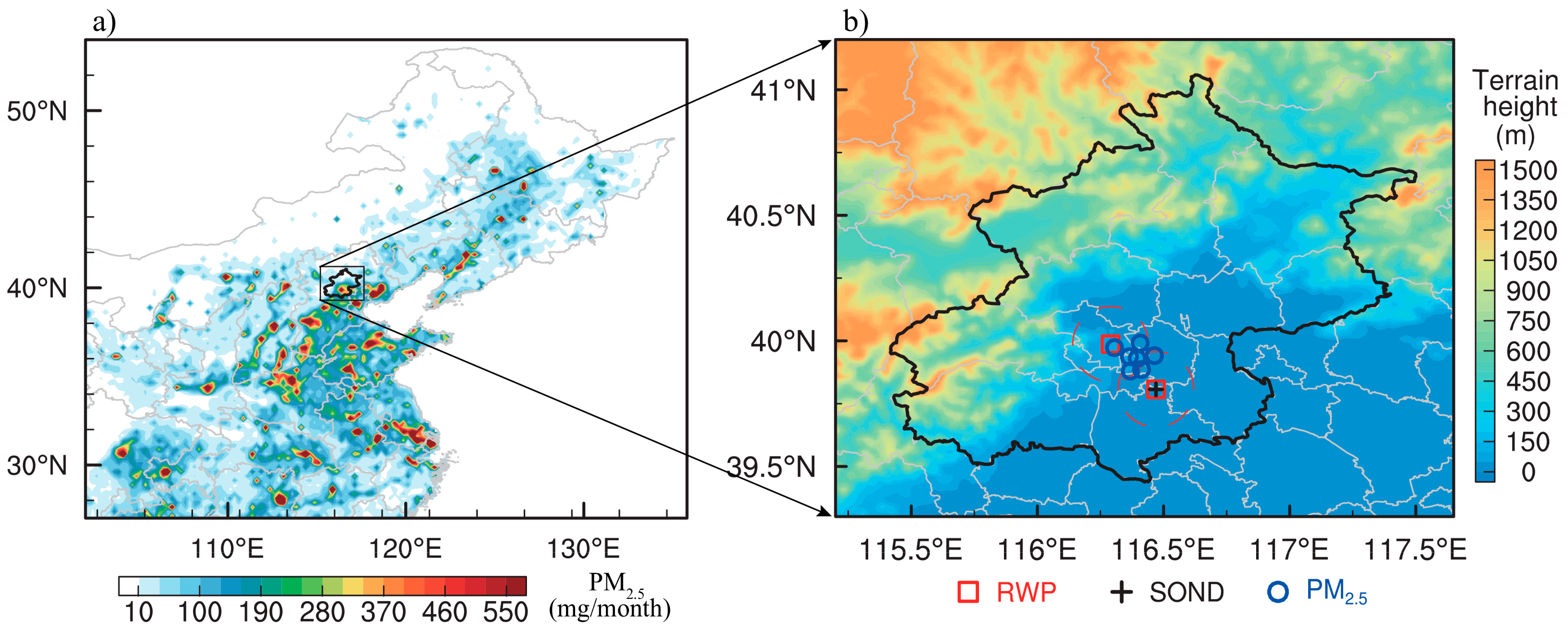
2.1. Study Area

Beijing, the capital of the People’s Republic of China, is located in the north part of the North China Plain (NCP) of China and covers an area of around 16,410 square kilometers. As shown in Figure 1a, there exists a large amount of aerosol emission sources surrounding Beijing with the recent rapid economic development throughout China, especially in eastern China. Beijing is surrounded by the Yanshan Mountains to the north, and by Taihang Mountains to the west and northwestern (Figure 1b). In terms of the climate in Beijing, it typically belongs to a semi-humid continental climate in the north temperate zone, characterized by hot and humid summers due to the subsidence caused by the subtropical high, and cold, windy and dry winters which is mainly under the influence of the vast Siberian anticyclone [41,42,43]. Due to the huge amount of anthropogenic emission in the NCP (see Figure 1a), the atmospheric pollution (especially the PM2.5) in Beijing has been intensively analyzed in recent years [38,39,41,44].

2.2. Radar Wind Profiler Measurements

The RWP is a type of remote sensing instrument that detects and processes vertical-resolved wind field information by transmitting and receiving electromagnetic beams in different directions. This instrument can provide a variety of data products, including the profiles of horizontal wind speed and direction, and vertical velocity. Specifically, the RWP data used here were collected from two sites (marked by the red squares in Figure 1b), including the Tongzhou site (116.29° E; 39.99° N) and Chaoyang site (116.47° E; 39.81° N). Both RWPs deployed in Beijing are the CFL-16 profiler, which provides 25 levels of wind speed and direction below ~3 km above ground level (AGL) with a vertical resolution of 120 m, beginning at 150 m (AGL). The measurements of wind are taken at 6 min intervals, and the detailed specifications of the RWP are given in Table 1. Prior to further analysis, the raw data have to undergo strict quality control for data consistency, continuity, and deviation [41,45,46]. To match the hourly PM2.5, the original 6-min RWP measurements were aggregated into hourly data. Our study period covers the whole boreal winter of 2018 (December of 2018 through February of 2019). To exclude the effect of wet deposition, all the measurements mentioned in this study refer to those taken on non-precipitation (i.e., rain, hail, or snow) hours, unless otherwise noted. The hourly precipitation events with precipitation amounts larger than 0.1 mm are generally defined as precipitation hours [44].

2.3. Ground-level PM2.5 Concentration Measurements

In this study, the aerosol pollution in Beijing is denoted by hourly ground-level PM2.5 concentration measurements, collected from seven air quality sites (marked by the blue circles in Figure 1b; Table 2) of the Ministry of Ecology and Environment of China. At each monitoring site, the hourly PM2.5 is measured using the tapered element oscillating microbalance method and the beta absorption method. The systematic uncertainty of ground-level PM2.5 mass concentration at these air quality monitoring stations was controlled within 15% [47]. To avoid the uncertainties caused by aerosol heterogenous distribution, averages were taken on the PM2.5 measurements from all these seven sites.

2.4. Radiosonde and Other Meteorological Data

The radiosonde soundings routinely measured in Beijing (116.47° E; 39.80° N, marked by the black cross in Figure 1b) were also collected to characterize the temperature inversion in association with aerosol pollution. As stated in our previous studies [29,48], the sounding balloons in China are launched twice per day at around 0800 and 2000 Beijing time (BJT = UTC + 8 h). It follows that the sounding measurements at 0800 BJT were compared with the hourly RWP and PM2.5 data at 0800 BJT. As illustrated in Figure 1b, all these meteorological stations and PM2.5 monitoring sites are evenly distributed to represent the hourly meteorological conditions in the whole urban area of Beijing well.

2.5. Air Mass Back Trajectory Model

Air masses related to regional or synoptic meteorological conditions could be responsible for the atmospheric transport of aerosol particles in the vertical and horizontal directions [26,49]. As such, we identified the main transport pathways of aerosol pollutants from surrounding regions to Beijing using the Hybrid Single-Particle Lagrangian Integrated Trajectory Model (HYSPLIT) [50]. The HYSPLIT developed by the National Ocean and Atmospheric Administration (NOAA)’s Air Resources Laboratory has been extensively used for the analyses of transboundary transport and dispersion of aerosol [51]. Based on the HYSPLIT and The GDAS (Global Data Assimilation System) reanalysis data, the frequency distribution and cluster mean of 24-h backward trajectories of each day for the period from December 1, 2018, to February 28, 2019, were calculated, respectively. The trajectory endpoint was set in the urban area of Beijing (116.37 °E, 40.09 °N) with a height of 100 m above ground level (AGL).

2.6. Methodology

In order to avoid the effects induced by the seasonal variation of aerosol at specific sites and by the spatial variation among different sites within the same region, hourly PM2.5 concentrations for a given site are normalized using the monthly mean of each site and year according to the approach by Wang et al. [52]. The PM2.5 dataset is then grouped into three subsets, each of which has the same number of samples. The lower and upper terciles of normalized PM2.5 refer to the clean (bottom 1/3) and polluted (top 1/3) conditions, respectively. In this way, comparison analysis can be performed between clean and polluted atmospheric conditions, and good sampling statistics can be maintained [11,53], even though the critical threshold of normalized PM2.5, which is used to distinguish between the clean and polluted categories, differs by various time scales. Besides, hourly wind anomalies with 120 m resolution in the vertical are calculated and then used in the subsequent analyses in diurnal association with ground-level PM2.5 concentration. This allows us to do a more detailed analysis of the wind variation for various PM2.5 pollution levels.
The VWS has been found to play important roles in the dispersion of air pollutants, and thus was calculated here to check its effects on PM2.5 variability. Therefore, the bulk shear, which refers to the magnitude of the bulk vector difference (top minus bottom) divided by height [54,55,56], is calculated as follows:
V W S = ( u z 1 u z 2 ) 2 + ( v z 1 v z 2 ) 2 z 1 z 2 × 1000
where V W S is the vertical wind shear (units: m / s km ), u z 1 and u z 2 represent the zonal wind at the height of z 1 and z 2 , respectively; and v z 1 and v z 2 represent the meridional wind at the height of z 1 and z 2 . z 1 is the top height and z 2 is the bottom height.
To enhance the visual interpretation, daily 24-h period is divided into eight sub-period at 3-hour intervals, which is defined as follows [57,58]: late night (0000 – 0300 BJT), early morning (0300–0600 BJT), morning (0600–0900 BJT), late morning (0900–1200 BJT), early afternoon (1200–1500 BJT), late afternoon (1500–1800 BJT), evening (1800–2100 BJT), and night (2100–2400 BJT).
Additionally, the bivariate polar plot has been used, combining wind measurements from RWP and PM2.5 measurements in Beijing, which is expected to provide insight into the sophisticated relationship between wind and PM2.5 [59,60].

3. Results and Discussion

3.1. Thermodynamic and Meteorological Variables Related To PM2.5

Figure 2 shows the time series of observed daily PM2.5 concentrations with vertically thermodynamic (temperature) and dynamic (wind) variables in Beijing simultaneously observed for the period from December 2018 to February 2019. The heavy PM2.5 pollution tended to occur more frequently on the days with low near-surface wind speed, and warmer air at the top of PBL (Figure 2b,c), given the wintertime climatological PBL height of 1–1.5 km in Beijing [61]. This generally does not favor the vertical ventilation and horizontal dispersion of aerosols. For example, during the pollution episode from December 14, to 18 of 2018, the near-surface wind speed in Beijing was significantly lower than those of pre- and post-periods, which was accompanied by strong thermal inversion layer. The southerly winds prevailed in the lowest 1–2 km of PBL (Figure 2a), which tended to transport aerosol particles from Hebei, a significant source region of aerosol emission to the south of Beijing (Figure 1a).
The most severe haze episode occurred during the study period persisted at least three days, starting from 12 January 2019 until 14 January 2019, during which PM2.5 exceeded 100 μg m−3. A most extremely high concentration of greater than 200 μg m−3 was observed as well. Coincidently, there existed weak southwesterly winds, and strong temperature inversion in the PBL, both of which contributed to this atmospheric pollution.

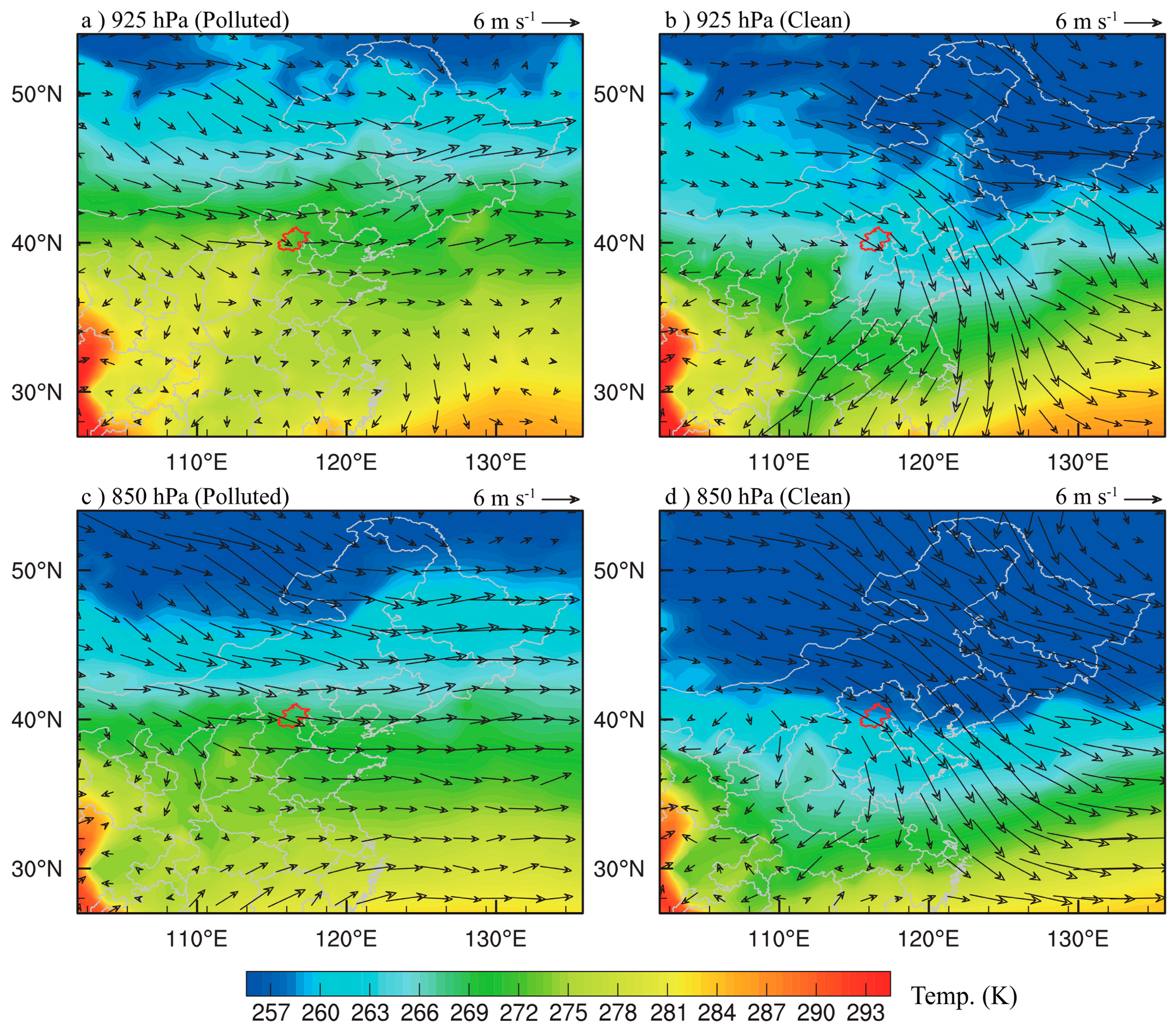
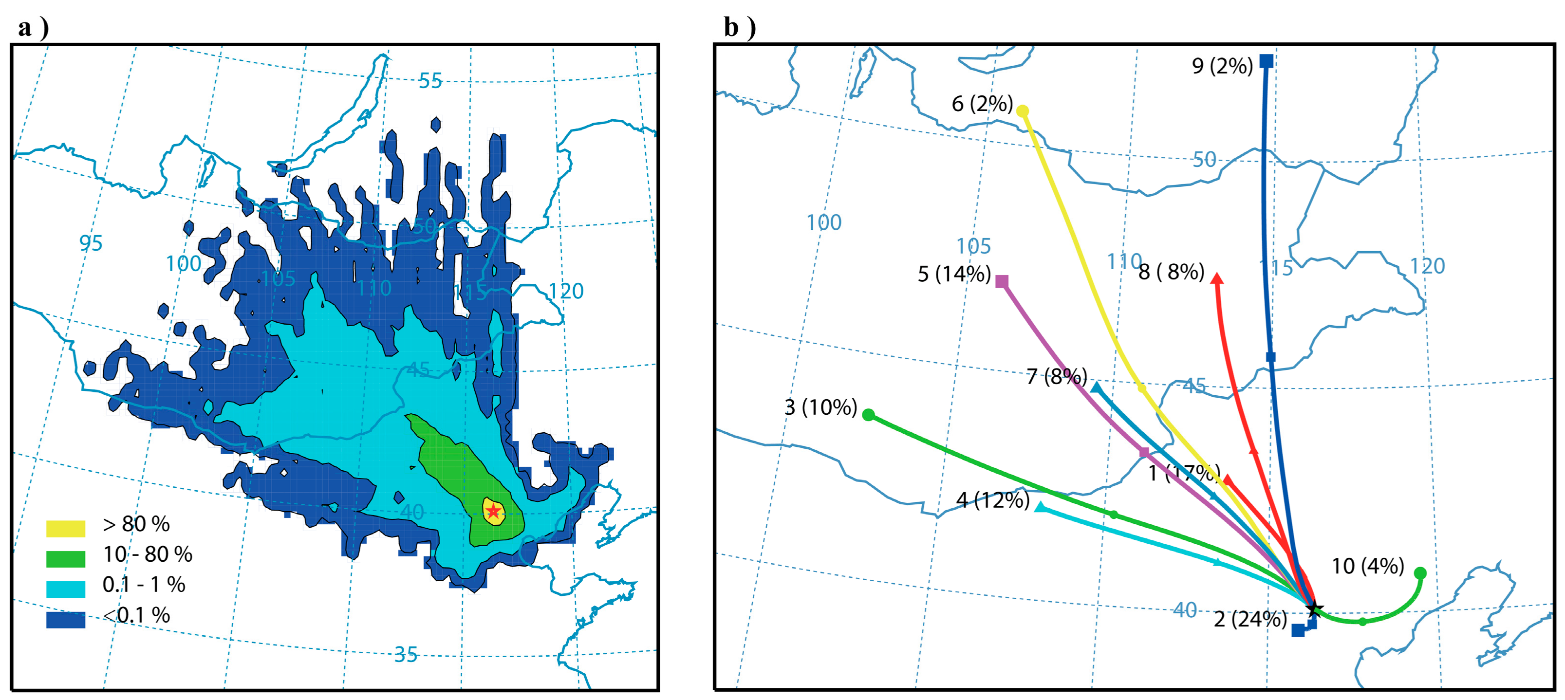
3.2. Synoptic-Scale Circulation and Backward Trajectory Statistical Analysis

In this section, we will examine the role of synoptic-scale meteorology underlying the polluted and clean episodes observed during the study period in Beijing. The first step to accomplish this is to determine the climatological wintertime winds at 925 hPa and 850 hPa pressure levels over Beijing and its surroundings. As shown in Figure 3a,c, weak westerly or southwesterly winds dominated both 850 hPa and 925 hPa pressure levels during the high aerosol-loading winter days in Beijing. By comparison, the wind fields at 850 hPa and 925 hPa were characterized by strong northwesterly winds over Beijing, which generally led to frequent intrusion of cold air mass (Figure 3b,d).
This cold advection could bring in cold and clean air from the northern regions without much anthropogenic emission sources (Figure 1a), thus resulting in low PM2.5 concentration in Beijing, such as the extremely clean atmospheric episode occurring during December 27 to 30, 2018 (Figure 2). By contrast, less lapse rate of temperature and southwesterly winds featured the synoptic conditions favoring the accumulation of PM2.5 (Figure 3a,c), well corroborating the vertical wind measurements in Beijing shown in Figure 2. Our findings were broadly consistent with the relationships between PM2.5 concentration, temperature, and wind speed in winter found in other regions of the NCP [62].
To further our understanding of the long-range transport to particulate matter pollution in Beijing, the 24-h backward trajectories were calculated and clustered. As illustrated in Figure 4, the prevailing northwesterly winds dominated the contribution in terms of transboundary transport (72% of all 24-h back trajectories). Interestingly, a small fraction of the trajectories (28%) came from the south, which was linked to most of the polluted episodes in Beijing during December 1, 2018, to February 28, 2019.

3.3. Diurnal Variations in Vertical Winds

Figure 5 illustrates the diurnal variations of wind speed and direction in Beijing for the heights ranging from ground-surface up to 3 km AGL under mean, polluted and clean conditions and their corresponding hodographs, and so do the anomalies of wind profile under polluted and clean conditions relative to the average wintertime winds in Beijing.
Overall, the mean wind speed was found to increase with height (Figure 5a). Meanwhile, the mean wind exhibited a pronounced diurnal cycle in the lower PBL (i.e., from the ground surface to 1 km AGL), and much stronger winds occurred during nighttime near the ground-surface compared with daytime (Figure 5a), which could be due to much reduced turbulence-related friction. This was also likely associated with the radiative (nocturnal) cooling in the night, which tended to reduce the eddy viscosity and momentum transfer from the upper levels, and in turn, lead to decreased wind speed [63]. However, the wind at the top of PBL or low troposphere exhibited double peaks: one is midnight and another in the later morning (1000 BJT). Under clean conditions, wind vector veered with the height between the near ground surface and 1 km AGL, followed by significant backing above 2 km (Figure 5b). Veering winds in the lowest layers of the atmosphere are most likely the result of friction-related processes while the backing winds are indicative of cold advection [64], which is mainly contributed by prevailing northwest winds (Figure 5a).
Under both polluted and clean conditions, the wind profiles showed significant diurnal variation at all heights, and its amplitude and sign differed greatly in the vertical during a daily cycle (Figure 5c,e), indicating that the lower part of PBL was characterized by prevailing southerly and northerly winds, respectively. The hodograph for polluted conditions exhibited smaller vertical shear at most heights, irrespective of the time of a day (Figure 5d). On the contrary, the curvature of the anticyclone rotation at above approximately 2 km AGL was significantly larger under clean conditions, resulting in larger wind shear (Figure 5f), which was most likely due to many more cold waves (Figure 2 and Figure 3d).
Also, there existed significant wind anomalies under polluted and clean conditions (Figure 5g,i). Coincidently, a clockwise turning of the wind with the height was observed near the ground surface under polluted condition (Figure 5h), which was indicative of a warm air advection from the south. In contrast, the backing winds were found near the ground surface under clean conditions (Figure 5j), confirming the notion of northerlies-induced decreases in aerosol concentration. This highlights the urgency of consideration of VWS and wind direction in the aerosol pollution and its formation causes. In particular, under polluted conditions, negative wind anomalies prevailed at almost all times of the day in the PBL over Beijing, especially during the nighttime, indicating aerosol-induced changes in radiation reaching the surface could be linked to the dramatical reduction of wind speed. By comparison, positive southerly wind anomalies emerged during 1000–2000 BJT in the troposphere above 1.75 km, indicating that there were strong elevated PM2.5 transport paths, which were located at the heights above the PBL at this time period. Under clean conditions (Figure 5c), positive northerly wind anomalies prevailed at almost all height, with the exception of negative wind anomalies above the PBL at roughly 0600, 1200, and 1900 BJT. This suggested that less aerosol tended to be associated with northerly winds, which further strengthened the role of cold advection from the northwestern parts of Beijing in reducing ground-level PM2.5.

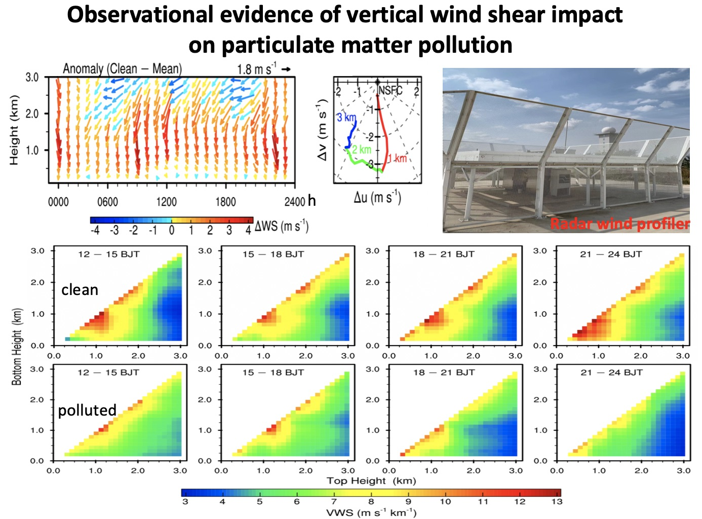
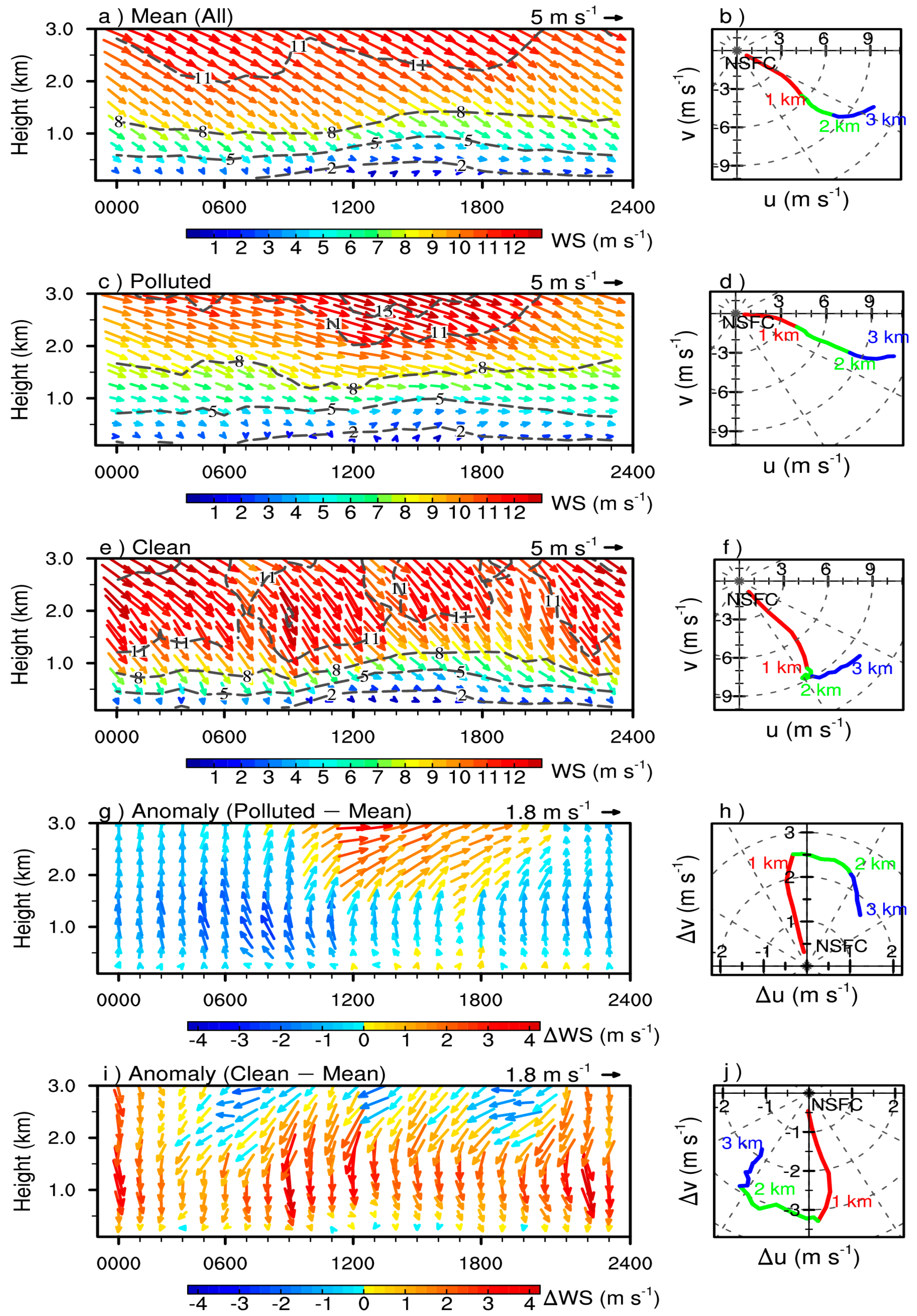
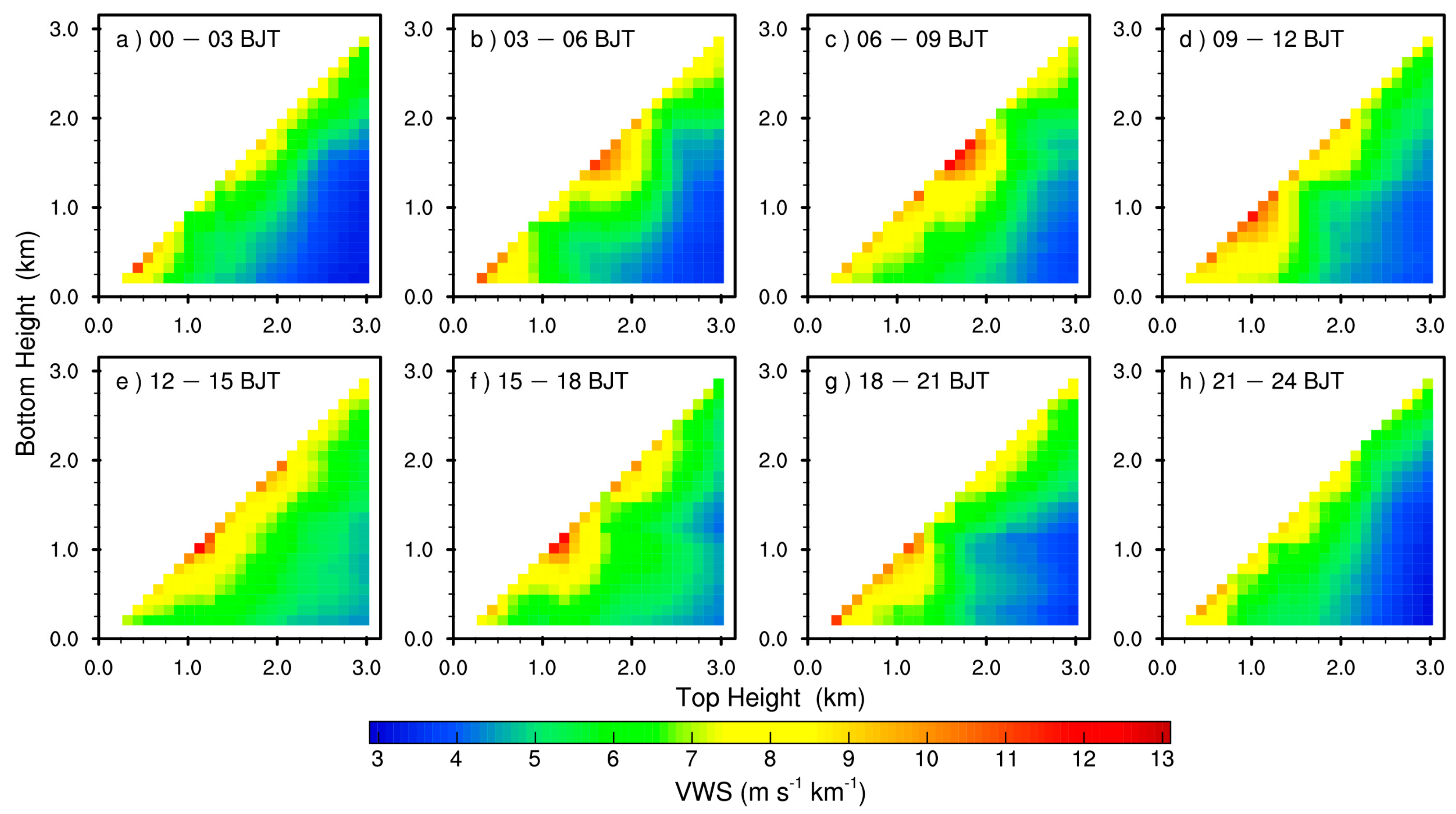
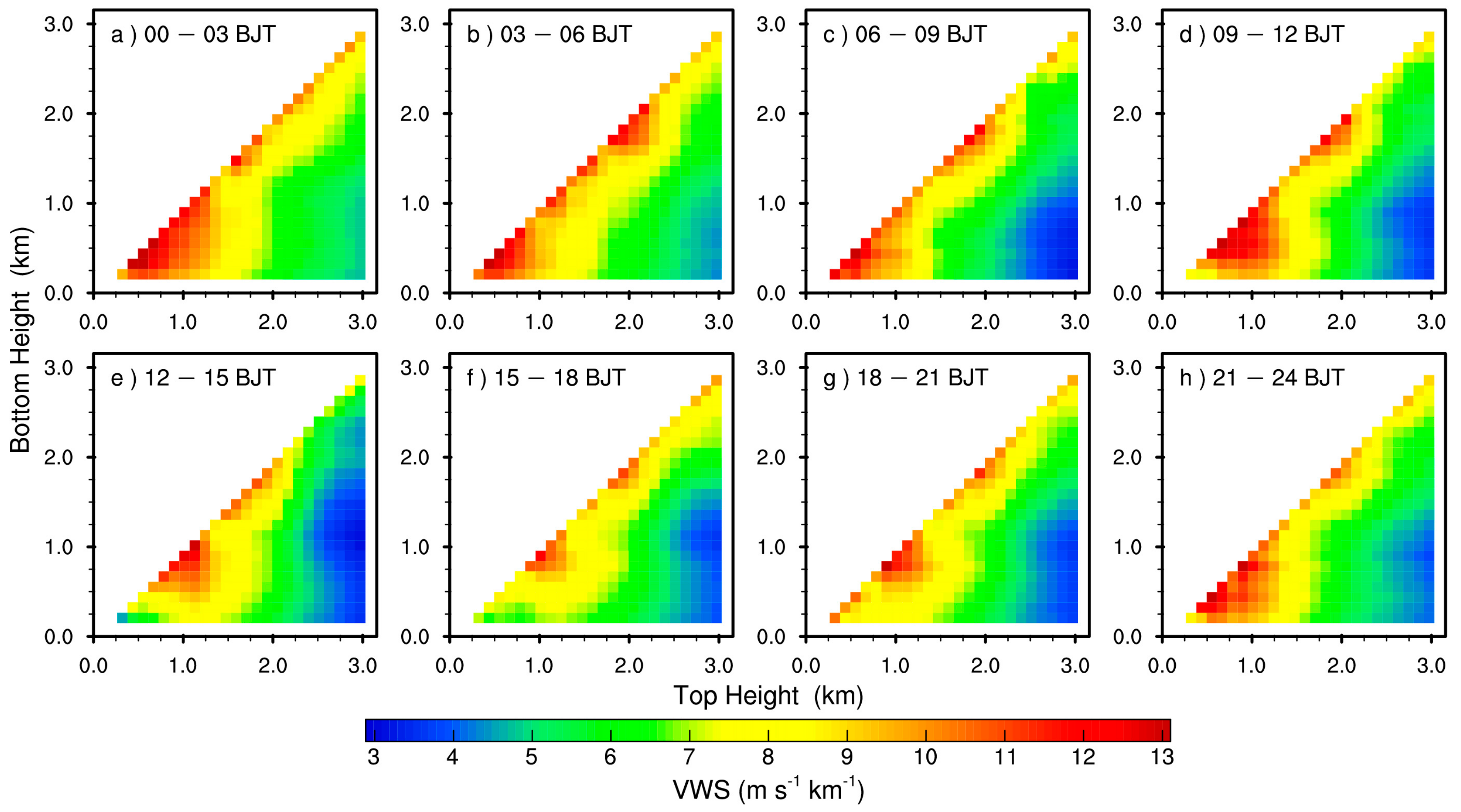
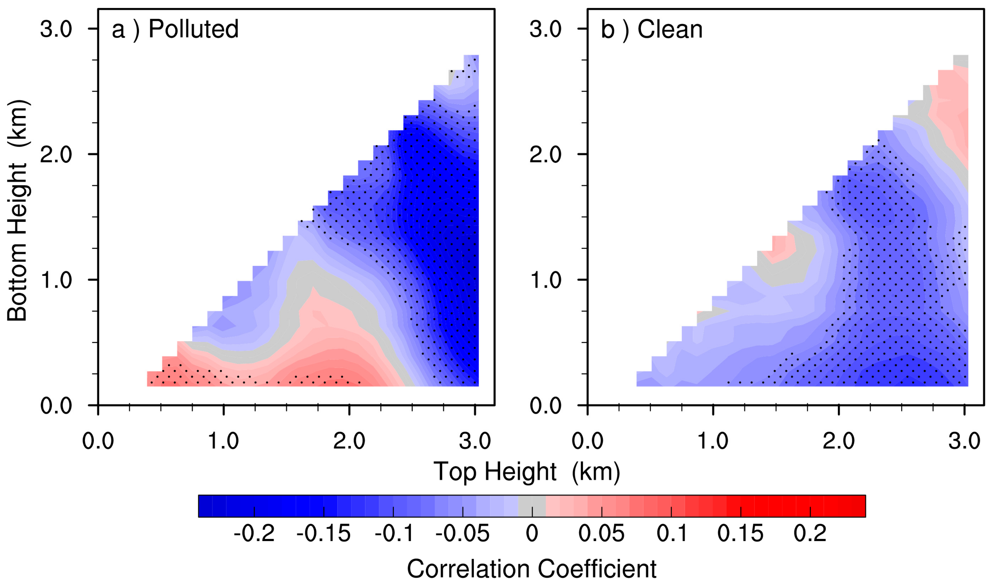
3.4. Vertical Wind Shear Under Polluted And Clean Condition

The vertical wind shear is known to be able to strongly influence the vertical mixing process and resultant changes in aerosol pollutants in the PBL [26]. Figure 6 and Figure 7 show the vertical distribution of VWS under polluted and clean conditions, respectively. The leading diagonal (top right to bottom left) denotes the local VWS at each level, whereas the shading in color indicates the magnitude of VWS at least two consecutive vertical levels. Note that VWS distribution does not take into account the shear direction.
Generally, the pattern of the diurnal cycle did not change much when the atmosphere evolved from clean to polluted conditions, except for the magnitude of VWS. The magnitude of VWS was found to be much smaller under polluted conditions than that under clean conditions, indicative of weaker vertical mixing in the presence of high aerosol concentration in the PBL. This, in turn, led to a stronger accumulation of ground-level PM2.5. On average, the local VWS for the polluted condition was ~8 m s−1 km−1, as compared to as high as ~10.5 m s−1 km−1 for the clean condition. However, note that the VWS for polluted conditions between 2.5–3 km and <1.5 km was greater than that under clean conditions during the afternoon (1200–1800 BJT), which could be related with the positive southerly wind vector anomalies above 2 km during 1200–1800 BJT (Figure 5b). It implied that strong wind in the upper level and in the PBL tended to transport PM2.5 from southern Hebei province to Beijing, further deteriorating the air quality in Beijing through these strongly vertical mixing exchanges (i.e., larger VWS) in the upper level and in the PBL. This finding was in agreement with the observational evidence from Hong Kong [26]. In addition, the magnitude of VWS (> 5 m s−1 km−1) was small during the night to morning (1800–1200 BJT) but large during the afternoon (1200–1800 BJT) under polluted conditions. On the contrary, under clean conditions, the VWS (> 5 m s−1 km−1) was relatively larger during the night (2100-0600 BJT) than during the day. These differences in diurnal variations of VWS (> 5 m s−1 km−1) under polluted/clean conditions were probably associated with different integrated effects of the local circulation (mountain-valley and urban heat island circulations) [14,32] and synoptic patterns [65,66].
Figure 8 presents the correlation between VWS at different layers and ground-level PM2.5 under polluted and clean conditions, respectively. It generally exhibits marked differences (even with opposite signs) in the lowest part of PBL in both conditions. In particular, the correlation coefficients seemed to be positive for the altitudes from the ground surface up to 2.5 km AGL under polluted conditions (Figure 8a), which meant the weak VWS near the ground surface or lower part of PBL observed in Figure 6 favored the accumulation of aerosol. In contrast, the correlation coefficient shifted from positive to negative as the VWS occurred upward, suggesting that the stronger VWS above the PBL was linked to lower ground-level PM2.5 concentration. Interestingly, under clean conditions, a ubiquitous negative correlation was found between VWS and ground-level PM2.5 in the almost whole lower atmosphere except in the height of 1 km and that above 2.5 km and beyond (Figure 8b). The increase of VWS tended to be accompanied by enhanced vertical mixing of aerosol, leading to reduced ground-level PM2.5, which could account for this negative correlation observed for the clean condition. The exception in height above 2.5 km could be associated with air mass intrusion of long-range transported aerosol episodes [67], given the dominant height of long-range transboundary transport being generally above the PBL [68,69,70].

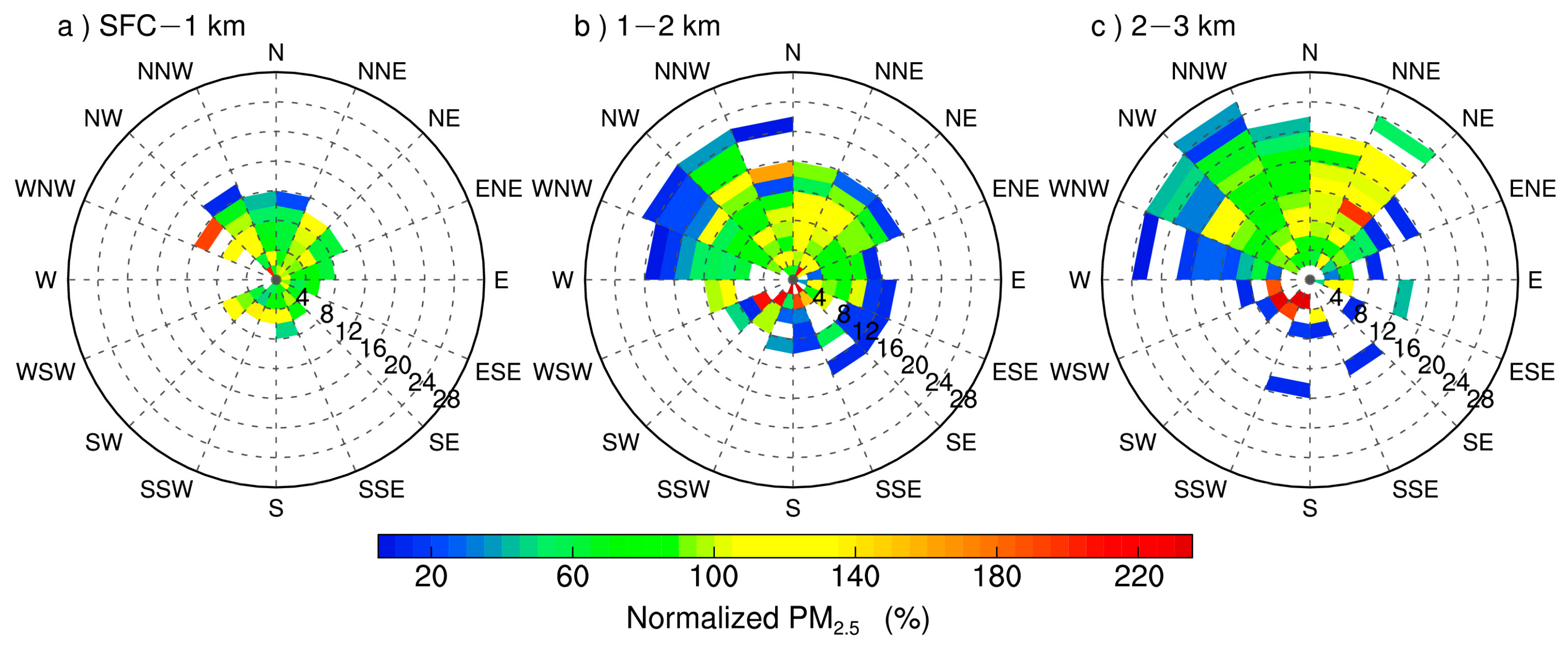
3.5. The Dependency of Ground-Level PM2.5 On Vertically Resolved Winds

The bivariate polar plots in Figure 9 showed that the normalized PM2.5 concentration (hereinafter referred to as NPM2.5) in Beijing varied by wind direction and speed at different heights, including ground-surface–1km, 1–2 km and 2–3 km. Specifically, at the height of ground surface–1km (Figure 9a), high aerosol concentration episodes (HEP, NPM2.5 > 120%) were observed when the cardinal winds occurred along the NNE–NE, and NNW–WNW directions with speeds of greater than 6 m s−1 and even up to 10 m s−1. Additionally, the polluted cases were observed when the prevailing cardinal winds were in the WSW–SSE sector with wind speed 4–6 m s−1, consistent with previous findings [71]. At the heights of 1–2 km, extreme HEPs (i.e., NPM2.5 >200 %) were observed mainly when winds blew along the SW–SE sector with a speed of <6 m s−1 (Figure 9b). By comparison, HPEs occurred when the NE–N winds prevailed at moderate to high wind speeds (4–12 m s−1). As the atmospheric height increased to 2–3km, HEP mainly occurred when the winds were coming from NE–N sector at high wind speed (12–20 m s−1), and also occurred in the NW sector with a wind speed of 14 m s−1 (Figure 9c). The surprisingly high NPM2.5 tended to occur in Beijing when the winds blew from WSW–S at weaker wind speeds (2–6 m s−1). In contrast, the NPM2.5 in the NW sector was found to be significantly reduced. In general, it was found that a smaller range of direction angle was accompanied by smaller wind shear at the lower part of the PBL, whereas stronger southerly wind prevailed with larger wind shear in the upper PBL and even above the PBL under heavy polluted conditions (Figure 5 and Figure 7).
The region to the south of Beijing was previously recognized to be a key emission source region for the PM2.5 pollution episodes in Beijing, especially southerly or southwesterly wind prevailed [72,73,74]. This, in part, was attributed to transboundary PM2.5 transport [28,75]. The results presented here provided convincing evidence that regional sources largely contribute to PM2.5 below 3 km, where existed kind of main PM2.5 transport path from south to Beijing, which basically agreed with the findings from model simulation analysis [76].
Another striking feature we observed here was that a few aerosol pollution episodes occurred even as the strong northerly or northwesterly winds dominated from the ground surface up to 3 km AGL (Figure 9). This could be likely linked to the long-range transported aerosol from northwestern or northeasten China, which was verified or corroborated in previous observational and model investigations [77].

4. Concluding Remarks

Based on continuous fine-resolution radar wind profiler (RWP) observations, radiosonde measurements during the winter for the period December of 2018 to February of 2019, the height-resolved wind vectors were analyzed, along with the impact of vertical wind shear on PM2.5 pollution in Beijing. The main findings are summarized as follows:
Overall, the diurnal variations in wind profiles were found to differ greatly when classified by different ground-level PM2.5 concentrations. Specifically, the southerly wind anomalies dominated throughout the whole PBL or even beyond the PBL under polluted conditions during the course of a day, in sharp contrast to the northerly wind anomalies in the PBL under clean condition. More strikingly, under pollution conditions, the positive anomaly of southerly wind speed mainly occurred at 1.75 km AGL during 1000–2000 BJT. This favored the transboundary transport originated from significant aerosol emission source to the south of Beijing, thereby leading to high ground-level PM2.5 concentration in Beijing.
Besides, the ground-level PM2.5 pollution exhibited a strong dependence on the vertical variation of the wind direction. The VWS tended to be much weaker in the lower PBL under polluted conditions, compared with under clean conditions, which could be strong ground-level PM2.5 accumulation induced by weak vertical mixing in the PBL. Notably, the PM2.5 pollution mainly appeared within the PBL as weak southerly winds prevailed when the relatively small VWS was observed as well. Above the PBL, strong northerlies winds also favored the long-range transport of aerosols, which in turn deteriorated the air quality in Beijing as well. This was well corroborated by the results from synoptic-scale circulation and backward trajectory analysis.
In summary, not only wind profiling but also the VWS at various heights could significantly modulate the ground-level PM2.5 concentrations. Also, the present work highlighted the role that the height-resolved wind shear plays in better understanding the wintertime aerosol pollution episodes in Beijing. To increase the generalizability of the reported associations between aerosol and VWS; nevertheless, more efforts have to be made to include a much longer time series of observations at larger spatial domains in the future. More importantly, more wind and VWS measurements from RWP are desperately needed to be assimilated into the air quality model, which is expected to have great implications for improving the wintertime air quality forecast in China.

Author Contributions

Conceptualization, J.G.; Methodology, J.G. and Y.Z.; Validation, J.G., Y.Y. and S.H.L.Y.; Formal Analysis, Y.Z., J.G. and Y.Y.; Data Curation, J.G., Y.Z.; Writing–Original Draft Preparation, Y.Z. and J.G.; Review & Editing, J.G., Y.Y., Y.Z. and Y.W.; Visualization, Y.Z.; Supervision, J.G. and Y.W.; Resources, J.G. and S.H.L.Y.; Funding Acquisition, J.G. All authors have read and agreed to the published version of the manuscript.

Funding

This work was supported by the National Natural Science Foundation of China (Grant 41771399), Ministry of Science and Technology of China (Grant 2017YFC1501401), Chinese Academy of Sciences (Grant GXDA20040502), and Chinese Academy of Meteorological Sciences (Grants 2017Z005).

Acknowledgments

We appreciated greatly the National Meteorological Information Center of China Meteorological Administration for providing the radar wind profiler (RWP) data (https://data.cma.cn/en/). We also sincerely appreciated the PM2.5 data made publicly accessible by the Ministry of Ecology and Environment of China (http://www.cnemc.cn/en/). Last but not least, the authors would like to thank the editor and three anonymous reviewers for their constructive comments which help improve the quality of our manuscript.

Conflicts of Interest

The authors declare no conflict of interest.

References

  1. Qu, Y.; Han, Y.; Wu, Y.; Gao, P.; Wang, T. Study of PBLH and its correlation with particulate matter from one-year observation over Nanjing, southeast China. Remote Sens. 2017, 9, 668. [Google Scholar] [CrossRef] [Green Version]
  2. Zhao, X.; Zhao, P.; Xu, J.; Meng, W.; Pu, W.; Dong, F.; He, D.; Shi, Q. Analysis of a winter regional haze event and its formation mechanism in the North China Plain. Atmos. Chem. Phys. 2013, 13, 5685–5696. [Google Scholar] [CrossRef] [Green Version]
  3. Lee, K.H.; Kim, J.E.; Kim, Y.J.; Kim, J.; von Hoyningen-Huene, W. Impact of the smoke aerosol from Russian forest fires on the atmospheric environment over Korea during May 2003. Atmos. Environ. 2005, 39, 85–99. [Google Scholar] [CrossRef]
  4. Tie, X.; Cao, J. Aerosol pollution in China: Present and future impact on environment. Particuology 2009, 7, 426–431. [Google Scholar] [CrossRef]
  5. Wang, L.; Wang, H.; Liu, J.; Gao, Z.; Yang, Y.; Zhang, X.; Li, Y.; Huang, M. Impacts of the near-surface urban boundary layer structure on PM2.5 concentrations in Beijing during winter. Sci. Total Environ. 2019, 669, 493–504. [Google Scholar] [CrossRef] [PubMed]
  6. Li, Z.; Lau, W.M.; Ramanathan, V.; Wu, G.; Ding, Y.; Manoj, M.; Liu, J.; Qian, Y.; Li, J.; Zhou, T. Aerosol and monsoon climate interactions over Asia. Rev. Geophys. 2016, 54, 866–929. [Google Scholar] [CrossRef]
  7. Li, Z.; Wang, Y.; Guo, J.; Zhao, C.; Cribb, M.C.; Dong, X.; Fan, J.; Gong, D.; Huang, J.; Jiang, M.; et al. East Asian Study of Tropospheric Aerosols and their Impact on Regional Clouds, Precipitation, and Climate (EAST-AIRCPC). J. Geophys. Res. Atmos. 2020, 124, 13026–13054. [Google Scholar] [CrossRef] [Green Version]
  8. Guo, J.; Deng, M.; Lee, S.S.; Wang, F.; Li, Z.; Zhai, P.; Liu, H.; Lv, W.; Yao, W.; Li, X. Delaying precipitation and lightning by air pollution over the Pearl River Delta. Part I: Observational analyses. J. Geophys. Res. Atmos. 2016, 121, 6472–6488. [Google Scholar] [CrossRef]
  9. Guo, J.; Xia, F.; Zhang, Y.; Liu, H.; Li, J.; Lou, M.; He, J.; Yan, Y.; Wang, F.; Min, M. Impact of diurnal variability and meteorological factors on the PM2.5-AOD relationship: Implications for PM2.5 remote sensing. Environ. Pollut. 2017, 221, 94–104. [Google Scholar] [CrossRef] [Green Version]
  10. Guo, J.; Su, T.; Li, Z.; Miao, Y.; Li, J.; Liu, H.; Xu, H.; Cribb, M.; Zhai, P. Declining frequency of summertime local-scale precipitation over eastern China from 1970 to 2010 and its potential link to aerosols. Geophys. Res. Lett. 2017, 44, 5700–5708. [Google Scholar] [CrossRef]
  11. Guo, J.; Liu, H.; Li, Z.; Rosenfeld, D.; Jiang, M.; Xu, W.; Jiang, J.H.; He, J.; Chen, D.; Min, M. Aerosol-induced changes in the vertical structure of precipitation: A perspective of TRMM precipitation radar. Atmos. Chem. Phys. 2018, 18, 13329–13343. [Google Scholar] [CrossRef] [Green Version]
  12. Rosenfeld, D.; Sherwood, S.; Wood, R.; Donner, L. Climate effects of aerosol-cloud interactions. Science 2014, 343, 379–380. [Google Scholar] [CrossRef] [PubMed]
  13. Wang, Q.; Li, Z.; Guo, J.; Zhao, C.; Cribb, M. The climate impact of aerosols on the lightning flash rate: Is it detectable from long-term measurements? Atmos. Chem. Phys. 2018, 18, 12797–12816. [Google Scholar] [CrossRef] [Green Version]
  14. Yang, Y.; Zheng, Z.; Yim, S.Y.; Roth, M.; Ren, G.; Gao, Z.; Wang, T.; Li, Q.; Shi, C.; Ning, G. PM2.5 Pollution Modulates Wintertime Urban-Heat-Island Intensity in the Beijing-Tianjin-Hebei Megalopolis, China. Geophys. Res. Lett. 2020, 47. [Google Scholar] [CrossRef] [Green Version]
  15. Yang, Y.-J.; Wang, H.; Chen, F.; Zheng, X.; Fu, Y.; Zhou, S. TRMM-Based Optical and Microphysical Features of Precipitating Clouds in Summer Over the Yangtze–Huaihe River Valley, China. Pure Appl. Geophys. 2019, 176, 357–370. [Google Scholar] [CrossRef]
  16. Gu, Y.; Wong, T.W.; Law, C.; Dong, G.H.; Ho, K.F.; Yang, Y.; Yim, S.H.L. Impacts of sectoral emissions in China and the implications: Air quality, public health, crop production, and economic costs. Environ. Res. Lett. 2018, 13, 084008. [Google Scholar] [CrossRef]
  17. Yin, P.; Guo, J.; Wang, L.; Fan, W.; Lu, F.; Guo, M.; Moreno, S.; Wang, Y.; Wang, H.; Zhou, M.; et al. Higher risk of cardiovascular disease associated with smaller size-fractioned particulate matter. Environ. Sci. Technol. Lett. 2020. [Google Scholar] [CrossRef]
  18. Liu, C.; Chen, R.; Sera, F.; Vicedo-Cabrera, A.M.; Guo, Y.; Tong, S.; Coelho, M.S.Z.S.; Saldiva, P.H.N.; Lavigne, E.; Matus, P.; et al. Ambient Particulate Air Pollution and Daily Mortality in 652 Cities. N. Engl. J. Med. 2019, 381, 705–715. [Google Scholar] [CrossRef]
  19. Cohen, A.J.; Brauer, M.; Burnett, R.; Anderson, H.R.; Frostad, J.; Estep, K.; Balakrishnan, K.; Brunekreef, B.; Dandona, L.; Dandona, R.; et al. Estimates and 25-year trends of the global burden of disease attributable to ambient air pollution: An analysis of data from the Global Burden of Diseases Study 2015. Lancet 2017, 389, 1907–1918. [Google Scholar] [CrossRef] [Green Version]
  20. Li, Z.; Guo, J.; Ding, A.; Liao, H.; Liu, J.; Sun, Y.; Wang, T.; Xue, H.; Zhang, H.; Zhu, B. Aerosol and boundary-layer interactions and impact on air quality. Natl. Sci. Rev. 2017, 4, 810–833. [Google Scholar] [CrossRef]
  21. Zhang, Q.; Zheng, Y.; Tong, D.; Shao, M.; Wang, S.; Zhang, Y.; Xu, X.; Wang, J.; He, H.; Liu, W. Drivers of improved PM2.5 air quality in China from 2013 to 2017. Proc. Natl. Acad. Sci. USA 2019, 116, 24463–24469. [Google Scholar] [CrossRef] [PubMed] [Green Version]
  22. Chen, H.; Wang, H. Haze days in North China and the associated atmospheric circulations based on daily visibility data from 1960 to 2012. J. Geophys. Res. Atmos. 2015, 120, 5895–5909. [Google Scholar] [CrossRef]
  23. Chen, S.; Guo, J.; Song, L.; Li, J.; Liu, L.; Cohen, J.B. Inter-annual variation of the spring haze pollution over the North China Plain: Roles of atmospheric circulation and sea surface temperature. Int. J. Climatol. 2019, 39, 783–798. [Google Scholar] [CrossRef]
  24. Miao, Y.; Guo, J.; Liu, S.; Liu, H.; Zhang, G.; Yan, Y.; He, J. Relay transport of aerosols to Beijing-Tianjin-Hebei region by multi-scale atmospheric circulations. Atmos. Environ. 2017, 165, 35–45. [Google Scholar] [CrossRef]
  25. Yang, Y.; Zheng, X.; Gao, Z.; Wang, H.; Wang, T.; Li, Y.; Lau, G.N.; Yim, S.H. Long-term trends of persistent synoptic circulation events in planetary boundary layer and their relationships with haze pollution in winter half year over eastern China. J. Geophys. Res. Atmos. 2018, 123, 10,991–11,007. [Google Scholar] [CrossRef]
  26. Yang, Y.; Yim, S.H.; Haywood, J.; Osborne, M.; Chan, J.C.; Zeng, Z.; Cheng, J.C. Characteristics of Heavy Particulate Matter Pollution Events Over Hong Kong and Their Relationships With Vertical Wind Profiles Using High-Time-Resolution Doppler Lidar Measurements. J. Geophys. Res. Atmos. 2019, 124, 9609–9623. [Google Scholar] [CrossRef] [Green Version]
  27. Tai, A.P.; Mickley, L.J.; Jacob, D.J. Correlations between fine particulate matter (PM2.5) and meteorological variables in the United States: Implications for the sensitivity of PM2.5 to climate change. Atmos. Environ. 2010, 44, 3976–3984. [Google Scholar] [CrossRef]
  28. Li, J.; Du, H.; Wang, Z.; Sun, Y.; Yang, W.; Li, J.; Tang, X.; Fu, P. Rapid formation of a severe regional winter haze episode over a mega-city cluster on the North China Plain. Environ. Pollut. 2017, 223, 605–615. [Google Scholar] [CrossRef] [PubMed]
  29. Guo, J.; Li, Y.; Cohen, J.B.; Li, J.; Chen, D.; Xu, H.; Liu, L.; Yin, J.; Hu, K.; Zhai, P. Shift in the temporal trend in boundary layer height trend in China using long-term (1979–2016) radiosonde data. Geophys. Res. Lett. 2019, 46, 6080–6089. [Google Scholar] [CrossRef] [Green Version]
  30. Lou, M.; Guo, J.; Wang, L.; Xu, H.; Chen, D.; Miao, Y.; Lv, Y.; Li, Y.; Guo, X.; Ma, S. On the relationship between aerosol and boundary layer height in summer in China under different thermodynamic conditions. Earth Space Sci. 2019, 6, 887–901. [Google Scholar] [CrossRef] [Green Version]
  31. Zheng, Z.; Li, Y.; Wang, H.; Ding, H.; Li, Y.; Gao, Z.; Yang, Y. Re-evaluating the variation in trend of haze days in the urban areas of Beijing during a recent 36-year period. Atmos. Sci. Lett. 2019, 20, e878. [Google Scholar] [CrossRef]
  32. Zheng, Z.; Ren, G.; Wang, H.; Dou, J.; Gao, Z.; Duan, C.; Li, Y.; Ngarukiyimana, J.P.; Zhao, C.; Cao, C. Relationship between fine-particle pollution and the urban heat island in Beijing, China: Observational evidence. Bound. Layer Meteor. 2018, 169, 93–113. [Google Scholar] [CrossRef]
  33. Yang, Q.; Yuan, Q.; Li, T.; Shen, H.; Zhang, L. The relationships between PM2.5 and meteorological factors in China: Seasonal and regional variations. Inter. J. Env. Res. Pub. Heal. 2017, 14, 1510. [Google Scholar] [CrossRef] [PubMed] [Green Version]
  34. He, L.J.; Lin, A.W.; Chen, X.X.; Zhou, H.; Zhou, Z.G.; He, P.P. Assessment of MERRA-2 Surface PM2.5 over the Yangtze River Basin: Ground-based Verification, Spatiotemporal Distribution and Meteorological Dependence. Remote Sens. 2019, 11, 460. [Google Scholar] [CrossRef] [Green Version]
  35. Miao, Y.; Liu, S.; Guo, J.; Yan, Y.; Huang, S.; Zhang, G.; Zhang, Y.; Lou, M. Impacts of meteorological conditions on wintertime PM 2.5 pollution in Taiyuan, North China. Environ. Sci. Pollut. R. 2018, 25, 21855–21866. [Google Scholar] [CrossRef]
  36. Quan, J.; Tie, X.; Zhang, Q.; Liu, Q.; Li, X.; Gao, Y.; Zhao, D. Characteristics of heavy aerosol pollution during the 2012–2013 winter in Beijing, China. Atmos. Environ. 2014, 88, 83–89. [Google Scholar] [CrossRef]
  37. Tie, X.; Zhang, Q.; He, H.; Cao, J.; Han, S.; Gao, Y.; Li, X.; Jia, X.C. A budget analysis of the formation of haze in Beijing. Atmos. Environ. 2015, 100, 25–36. [Google Scholar] [CrossRef]
  38. Zhu, X.; Tang, G.; Guo, J.; Hu, B.; Song, T.; Wang, L.; Xin, J.; Gao, W.; Münkel, C.; Schäfer, K. Mixing layer height on the North China Plain and meteorological evidence of serious air pollution in southern Hebei. Atmos. Chem. Phys. 2018, 18, 4897–4910. [Google Scholar] [CrossRef] [Green Version]
  39. Chen, Y.; An, J.L.; Lin, J.; Sun, Y.L.; Wang, X.Q.; Wang, Z.F.; Duan, J. Observation of nocturnal low-level wind shear and particulate matter in urban Beijing using a Doppler wind lidar. Atmos. Ocean. Sci. Lett. 2017, 10, 411–417. [Google Scholar] [CrossRef] [Green Version]
  40. Liu, X.; Li, J.; Qu, Y.; Han, T.; Hou, L.; Gu, J.; Chen, C.; Yang, Y.; Liu, X.; Yang, T. Formation and evolution mechanism of regional haze: A case study in the megacity Beijing, China. Atmos. Chem. Phys. 2013, 13, 4501–4514. [Google Scholar] [CrossRef] [Green Version]
  41. Liu, B.; Ma, Y.; Guo, J.; Gong, W.; Zhang, Y.; Mao, F.; Li, J.; Guo, X.; Shi, Y. Boundary layer heights as derived from ground-based Radar wind profiler in Beijing. IEEE Trans. Geosci. Remote Sens. 2019, 57, 8095–8104. [Google Scholar] [CrossRef]
  42. Cai, W.; Li, K.; Liao, H.; Wang, H.; Wu, L. Weather conditions conducive to Beijing severe haze more frequent under climate change. Nat. Clim. Chang. 2017, 7, 257. [Google Scholar] [CrossRef]
  43. Pei, L.; Yan, Z.; Sun, Z.; Miao, S.; Yao, Y. Increasing persistent haze in Beijing: Potential impacts of weakening East Asian winter monsoons associated with northwestern Pacific sea surface temperature trends. Atmos. Chem. Phys. 2018, 18, 3173–3183. [Google Scholar] [CrossRef] [Green Version]
  44. Guo, J.; Deng, M.; Fan, J.; Li, Z.; Chen, Q.; Zhai, P.; Dai, Z.; Li, X. Precipitation and air pollution at mountain and plain stations in northern China: Insights gained from observations and modeling. J. Geophys. Res. Atmos. 2014, 119, 4793–4807. [Google Scholar] [CrossRef]
  45. Miao, Y.; Guo, J.; Liu, S.; Wei, W.; Zhang, G.; Lin, Y.; Zhai, P. The climatology of low-level jet in Beijing and Guangzhou, China. J. Geophys. Res. Atmos. 2018, 123, 2816–2830. [Google Scholar] [CrossRef]
  46. Wei, W.; Zhang, H.; Ye, X. Comparison of low-level jets along the north coast of China in summer. J. Geophys. Res. Atmos. 2014, 119, 9692–9706. [Google Scholar] [CrossRef]
  47. Operating Manual, TEOM Series 1400a Ambient Particulate Monitor; Thermo Fisher Scientific Inc.: Franklin, MA, USA, 2007.
  48. Guo, J.; Miao, Y.; Zhang, Y.; Liu, H.; Li, Z.; Zhang, W.; He, J.; Lou, M.; Yan, Y.; Bian, L. The climatology of planetary boundary layer height in China derived from radiosonde and reanalysis data. Atmos. Chem. Phys. 2016, 16, 13309. [Google Scholar] [CrossRef] [Green Version]
  49. Guo, J.; Zhang, X.; Cao, C.; Che, H.; Liu, H.; Gupta, P.; Zhang, H.; Xu, M.; Li, X. Monitoring haze episodes over Yellow Sea by combining multi-sensor measurements. Int. J. Remot. Sens. 2010, 31, 4743–4755. [Google Scholar] [CrossRef]
  50. Draxler, R.; Hess, G. An overview of the HYSPLIT_4 modelling system for trajectories. Aust. Meteorol. Mag. 1998, 47, 295–308. [Google Scholar]
  51. Stein, A.F.; Draxler, R.R.; Rolph, G.D.; Stunder, B.J.; Cohen, M.D.; Ngan, F. NOAA’s HYSPLIT atmospheric transport and dispersion modeling system. B. Am. Meteorol. Soc. 2015, 96, 2059–2077. [Google Scholar] [CrossRef]
  52. Wang, X.; Dickinson, R.E.; Su, L.; Zhou, C.; Wang, K. PM2.5 pollution in China and how it has been exacerbated by terrain and meteorological conditions. Bull. Am. Meteoro. Soc. 2018, 99, 105–119. [Google Scholar] [CrossRef]
  53. Koren, I.; Altaratz, O.; Remer, L.A.; Feingold, G.; Martins, J.V.; Heiblum, R.H. Aerosol-induced intensification of rain from the tropics to the mid-latitudes. Nat. Geosci. 2012, 5, 118. [Google Scholar] [CrossRef]
  54. Li, X.; Guo, X.; Fu, D. TRMM-retrieved cloud structure and evolution of MCSs over the northern South China Sea and impacts of CAPE and vertical wind shear. Adv. Atmos. Sci. 2013, 30, 77–88. [Google Scholar] [CrossRef]
  55. Markowski, P.; Richardson, Y. On the classification of vertical wind shear as directional shear versus speed shear. Weather Forecast. 2006, 21, 242–247. [Google Scholar] [CrossRef] [Green Version]
  56. Thompson, R.L.; Mead, C.M.; Edwards, R. Effective storm-relative helicity and bulk shear in supercell thunderstorm environments. Weather Forecast. 2007, 22, 102–115. [Google Scholar] [CrossRef]
  57. Guo, J.; Zhai, P.; Wu, L.; Cribb, M.; Li, Z.; Ma, Z.; Wang, F.; Chu, D.; Wang, P.; Zhang, J. Diurnal variation and the influential factors of precipitation from surface and satellite measurements in Tibet. Int. J. Climatol. 2014, 34, 2940–2956. [Google Scholar] [CrossRef]
  58. Singh, P.; Nakamura, K. Diurnal variation in summer precipitation over the central Tibetan Plateau. J. Geophys. Res. Atmos. 2009, 114. [Google Scholar] [CrossRef]
  59. Carslaw, D.C.; Beevers, S.D.; Ropkins, K.; Bell, M.C. Detecting and quantifying aircraft and other on-airport contributions to ambient nitrogen oxides in the vicinity of a large international airport. Atmos. Environ. 2006, 40, 5424–5434. [Google Scholar] [CrossRef]
  60. Westmoreland, E.J.; Carslaw, N.; Carslaw, D.C.; Gillah, A.; Bates, E. Analysis of air quality within a street canyon using statistical and dispersion modelling techniques. Atmos. Environ. 2007, 41, 9195–9205. [Google Scholar] [CrossRef]
  61. Zhang, W.; Guo, J.; Miao, Y.; Liu, H.; Li, Z.; Zhai, P. Planetary boundary layer height from CALIOP compared to radiosonde over China. Atmos. Chem. Phys. 2016, 16, 9951–9963. [Google Scholar] [CrossRef] [Green Version]
  62. Zhang, H.; Wang, Y.; Hu, J.; Ying, Q.; Hu, X.-M. Relationships between meteorological parameters and criteria air pollutants in three megacities in China. Environ. Res. 2015, 140, 242–254. [Google Scholar] [CrossRef] [PubMed]
  63. Yu, R.; Li, J.; Chen, H. Diurnal variation of surface wind over central eastern China. Climate Dyn. 2009, 33, 1089. [Google Scholar] [CrossRef]
  64. Doswell III, C.A. A review for forecasters on the application of hodographs to forecasting severe thunderstorms. Natl. Wea. Dig. 1991, 16, 2–16. [Google Scholar]
  65. Miao, Y.; Guo, J.; Liu, S.; Liu, H.; Li, Z.; Zhang, W.; Zhai, P. Classification of summertime synoptic patterns in Beijing and their associations with boundary layer structure affecting aerosol pollution. Atmos. Chem. Phys. 2017, 17, 3097–3110. [Google Scholar] [CrossRef] [Green Version]
  66. Liu, L.; Guo, J.; Miao, Y.; Li, J.; Chen, D.; He, J.; Cui, C. Elucidating the relationship between aerosol concentration and summertime boundary layer structure in central China. Environ. Pollut. 2018, 241, 646–653. [Google Scholar] [CrossRef]
  67. Raveh-Rubin, S. Dry intrusions: Lagrangian climatology and dynamical impact on the planetary boundary layer. J. Climate 2017, 30, 6661–6682. [Google Scholar] [CrossRef]
  68. Schaub, D.; Weiss, A.; Kaiser, J.; Petritoli, A.; Richter, A.; Buchmann, B.; Burrows, J. A transboundary transport episode of nitrogen dioxide as observed from GOME and its impact in the Alpine region. Atmos. Chem. Phys. 2005, 5, 23–37. [Google Scholar] [CrossRef] [Green Version]
  69. Huang, J.; Guo, J.; Wang, F.; Liu, Z.; Jeong, M.J.; Yu, H.; Zhang, Z. CALIPSO inferred most probable heights of global dust and smoke layers. J. Geophys. Res. Atmos. 2015, 120, 5085–5100. [Google Scholar] [CrossRef]
  70. Gu, Y.; Yim, S. The air quality and health impacts of domestic trans-boundary pollution in various regions of China. Environ. Int. 2016, 97, 117–124. [Google Scholar] [CrossRef] [PubMed]
  71. Chen, Y.; Schleicher, N.; Fricker, M.; Cen, K.; Liu, X.-l.; Kaminski, U.; Yu, Y.; Wu, X.-f.; Norra, S. Long-term variation of black carbon and PM2.5 in Beijing, China with respect to meteorological conditions and governmental measures. Environ. Pollut. 2016, 212, 269–278. [Google Scholar] [CrossRef] [PubMed]
  72. Lv, B.; Liu, Y.; Yu, P.; Zhang, B.; Bai, Y. Characterizations of PM2.5 pollution pathways and sources analysis in four large cities in China. Aerosol Air Qual. Res. 2015, 15, 1836–1843. [Google Scholar] [CrossRef]
  73. Wang, L.; Liu, Z.; Sun, Y.; Ji, D.; Wang, Y. Long-range transport and regional sources of PM2.5 in Beijing based on long-term observations from 2005 to 2010. Atmos. Res. 2015, 157, 37–48. [Google Scholar] [CrossRef]
  74. Zhang, Y.; Chen, J.; Yang, H.; Li, R.; Yu, Q. Seasonal variation and potential source regions of PM2.5-bound PAHs in the megacity Beijing, China: Impact of regional transport. Environ. Pollut. 2017, 231, 329–338. [Google Scholar] [CrossRef] [PubMed]
  75. Yang, Y.; Russell, L.M.; Lou, S.; Liao, H.; Guo, J.; Liu, Y.; Singh, B.; Ghan, S.J. Dust-wind interactions can intensify aerosol pollution over eastern China. Nat. Commun. 2017, 8, 15333. [Google Scholar] [CrossRef]
  76. Chen, H.; Li, J.; Ge, B.; Yang, W.; Wang, Z.; Huang, S.; Wang, Y.; Yan, P.; Li, J.; Zhu, L. Modeling study of source contributions and emergency control effects during a severe haze episode over the Beijing-Tianjin-Hebei area. Sci. China Chem. 2015, 58, 1403–1415. [Google Scholar] [CrossRef]
  77. Zhang, R.; Jing, J.; Tao, J.; Hsu, S.-C.; Wang, G.; Cao, J.; Lee, C.S.L.; Zhu, L.; Chen, Z.; Zhao, Y. Chemical characterization and source apportionment of PM2.5 in Beijing: Seasonal perspective. Atmos. Chem. Phys. 2013, 13, 7053–7074. [Google Scholar] [CrossRef] [Green Version]
Figure 1. The spatial distribution of (a) particulate particle with an aerodynamic diameter of 2.5 μm or less (PM2.5) emissions (mainly in the transportation, agriculture, industry, power and residual sectors) during winter in 2016, as acquired from the multi-resolution emission inventory for China (http://www.meicmodel.org/), and (b) monitoring stations in Beijing overlaid with topography (color shading). The red squares, blue circles, and black plus refer to the locations of radar wind profiler (RWP), PM2.5, and radiosonde (SOND) sites, respectively. The administrative boundary of Beijing is denoted by the black solid lines.
Remotesensing 12 00546 g001
Figure 2. (a) Time series of the horizontal averaged wind vectors as derived from the Radar Wind Profiler (RWP) in Beijing for the altitude ranges from the surface to 1 km (SFC–1 km), 1–2 km, and 2–3 km above ground level (AGL), which are denoted as the red, green, and blue vectors, respectively. The wind arrow is the direction towards which the wind is blowing, and the width of the wind vector is proportional to the wind speed. Time-height cross-sections of (b) potential temperature (PT, color shaded) from radiosonde measurements and (c) horizontal wind speed (color shaded) from RWP, overlaid with observed ground-level PM2.5 concentration (red lines). All these measurements were obtained at 0800 BJT during the period December 1, 2018, to February 28, 2019.
Remotesensing 12 00546 g002
Figure 3. Spatial distribution of the wind field (black arrows, vector), superimposed by temperature (shaded) at 925 hPa (a,b) and 850 hPa (c,d) pressure level under polluted (left column) and clean (right column) conditions, respectively. All data are from the National Center for Environmental Prediction (NCEP) global Final (FNL) reanalysis. The areas highlighted with red lines represent the region of interest (Beijing), which is the same as the region highlighted with black lines in Figure 1a.
Remotesensing 12 00546 g003
Figure 4. The spatial distribution of the trajectory frequency (a), and cluster-mean results of 24-h backward trajectories (b) calculated by the Hybrid Single-Particle Lagrangian Integrated Trajectory Model (HYSPLIT) ending at Beijing (116.37 °E; 40.09 °N, pentagram) at 100 m height AGL during winter from December 2018 to February 2019. The dots on the trajectories represent time node of 12h, and the percentage represents the ratio of the number of back trajectories in each cluster to the total number of back trajectories.
Remotesensing 12 00546 g004
Figure 5. Height-resolved diurnal variation of horizontal wind vector under all-sky mean (a), polluted (c) and clean (e) conditions, and their corresponding anomalies (relative to mean wind) under polluted (g) and clean (i) conditions in Beijing from December 1, 2018, to February 28, 2019. Also shown are their corresponding hodographs in the panels (b,d,f,h,j) on the right-hand sides. Note the vectors in panels (g)–(i) show the resultant wind anomaly direction, and the vector length and color indicate the magnitude of the resultant wind anomaly relative to the average wintertime winds in Beijing.
Remotesensing 12 00546 g005
Figure 6. Three-hourly averaged vertical wind shear (VWS) computed between different heights under polluted conditions in Beijing for (a) 0000–0300 BJT, (b) 0300–0600 BJT, (c) 0600–0900 BJT, (d) 0900–1200 BJT, (e) 1200–1500 BJT, (f) 1500–1800 BJT, (g) 1800–2100 BJT and (h) 2100–2400 BJT, during the period from December 2018 to February 2019. The X and Y axes represent the top and bottom height of the VWS bulk, respectively.
Remotesensing 12 00546 g006
Figure 7. Same as Figure 6 but under clean conditions.
Remotesensing 12 00546 g007
Figure 8. The correlation coefficient distribution between normalized ground-level PM2.5 and height-revolved VWS under (a) polluted and (b) clean conditions in Beijing. Gray dots indicate the Pearson correlation coefficient that is statistically significant at the 90% confidence level. The X and Y axes represent the top and bottom heights of the VWS bulk, respectively.
Remotesensing 12 00546 g008
Figure 9. Bivariate polar plot of normalized PM2.5 concentration (in percent) for the altitude ranges of (a) ground surface to 1 km (SFC–1km), (b) 1–2 km and (c) 2–3 km AGL during the period from December 1, 2018, to February 28, 2019. The wind directions are denoted by 16 compass direction: N, NNE, NE, ENE, E, ESE, SE, SSE, S, SSW, SW, WSW, W, WNW, NW, NNW. The radial axis represents wind speed in m s−1, which increases radially outward. The concentration of PM2.5 is scaled by colors.
Remotesensing 12 00546 g009
Table 1. Summary of the operating and sampling characteristics of the CFL-16 Radar Wind Profiler (RWP) deployed in Beijing.
ParameterRange of Respective Values
Direction accuracy≤ 10
Speed accuracy1 m s−1
Vertical resolution120 m
Lowest level150 m AGL
Maximum height16 km AGL
Operating frequency445 MHz
Aperture100 m2
Gain33 dB
Peak power23 kW
Pulse width0.8 us
Averaging time6~60 min
Table 2. Basic information for observation stations.
Station TypeStation
Name
PositionElevation (m)ObservationTime
Resolution
RWP54399116.29° E; 39.99° N46.9WS, WD1 hour
RWP54511116.47° E; 39.81° N32.5WS, WD1 hour
SNDBeijing (BJ)116.47° E; 39.81° N31.3T, P
(to calculate PT)
launched twice a day at 0715 and 1915 BJT
MEEHaidian (HD)116.32° E; 39.99° N-PM2.51 hour
MEEAoti (AT)116.41° E; 40.00° N-PM2.51 hour
MEEGuanyuan (GY)116.36° E; 39.94° N-PM2.51 hour
MEEDongsi (DS)116.43° E; 39.95° N-PM2.51 hour
MEEWanshou (WS)116.37° E; 39.87° N-PM2.51 hour
MEENongzhanguan (NZG)116.47° E; 39.97° N-PM2.51 hour
MEETiantan (TT)116.43° E; 39.87° N-PM2.51 hour
Note that RWP (Radar Wind Profiler), MEE (Ministry of Ecology and Environment), and SND (Radiosonde) stand for wind-profiler site, air quality site of the Ministry of Ecology and Environment, and radiosonde site, respectively. (WS: wind speed; WD: wind direction; Temperature: T; Pressure: P; Potential temperature: PT; Aerodynamic diameter smaller than 2.5 μm: PM2.5).

