First Evidence of Mesoscale Ocean Eddies Signature in GNSS Reflectometry Measurements

Abstract

Feasibility of sensing mesoscale ocean eddies using spaceborne Global Navigation Satellite Systems-Reflectometry (GNSS-R) measurements is demonstrated for the first time. Measurements of Cyclone GNSS (CYGNSS) satellite missions over the eddies, documented in the Aviso eddy trajectory atlas, are studied. The investigation reports on the evidence of normalized bistatic radar cross section (${\sigma }^0$) responses over the center or the edges of the eddies. A statistical analysis using profiles over eddies in 2017 is carried out. The potential contributing factors leaving the signature in the measurements are discussed. The analysis of GNSS-R observations collocated with ancillary data from the European Centre for Medium-Range Weather Forecasts (ECMWF) Reanalysis-5 (ERA-5) shows strong inverse correlations of ${\sigma }^0$ with the sensible heat flux and surface stress in certain conditions.

1. Introduction

Mesoscale ocean eddies can drive atmosphere response at mesoscales mainly through heat fluxes [1] and they have a local influence on near-surface wind, cloud properties, and rainfall [2]. Analysis of mesoscale eddy-atmosphere interactions from general circulation models suggests significant intermodel differences mainly stemming from two factors: surface wind strength and marine atmospheric boundary layer adjustments to mesoscale heat flux anomalies [3]. Several Earth-observing satellites have been aiding these models for decades with their data products.

Global Navigation Satellite System Reflectometry (GNSS-R) is a relatively new Earth observation technique for monitoring a large variety of geophysical parameters (see [4,5] for a review). This technique exploits the GNSS signals of opportunity after being reflected from the Earth’s surface, both over lands and oceans. The signals are intercepted by low-cost, low-power and low-mass GNSS-R receivers and are processed to extract geophysical information. These receivers onboard small low Earth-orbiting satellites offer cost-effective Earth observations with high coverage and unprecedented sampling rate. Cyclone GNSS (CYGNSS) is the satellite constellation consisting of eight microsatellites with the main science objective of ocean wind speed monitoring especially during hurricane events, launched in December 2016 [6].

Ocean monitoring is one of the most mature spaceborne GNSS-R applications, with a proven capability of surface wind measurement [7,8,9]. Insignificant level of sensitivity to rain attenuation [10] and cost-effective observation frequency are the main advantageous characteristics motivating researchers to develop new ideas for additional applications over oceans [11,12,13], and for the development of future novel GNSS-R missions [14,15].

Remote sensing of oceanic features, e.g., eddies, based on high precision GNSS-R altimetric measurements, are being pursued. For instance, [16] deduced sea surface topography observations from the GNSS-R phase measurements onboard the German High Altitude Long Range (HALO) research aircraft. In an air-borne GNSS-R study, the so-called “Eddy Experiment”, the capabilities of the technique for ocean altimetry [17] and scatterometry [18] were additionally demonstrated. Nevertheless, the response of the measurements over mesoscale eddies is not yet characterized and documented, despite the available large datasets from recent GNSS-R satellite missions.

A high number of observations are provided by CYGNSS offering a possibility to study the feasibility of observing ocean eddies using GNSS-R measurements. This research focuses on the GNSS-R scatterometric observations (rather than in an altimetry configuration) and tries to characterize eddy signatures in those measurements for the first time. The data are empirically analyzed and the signatures and physical explanations are discussed. Following this introduction, Section 2 describes the datasets and the method. The results are reported and discussed in Section 3. Finally, concluding remarks are given in Section 4.

2. Data and Method

Four datasets are used for the analysis covering the period from March to December 2017. The main dataset consists of the CYGNSS GNSS-R measurements. The eight CYGNSS microsatellites are dispersed in 35${}^{°}$ inclined orbits with an altitude of ≈520 km. The onboard GNSS-R receivers are equipped with distinct channels measuring up to four simultaneous GPS signals after reflection from the ocean surface [19]. The corresponding data are available at different processing levels. Level 1 (L1) provides a variety of parameters including the calibrated measurements of bistatic radar cross section (BRCS) as well as the Normalized BRCS (NBRCS) ${\sigma }^0$. The L1 data are further processed into the 10 m referenced wind speed above the ocean surface at Level 2 (L2). For the analysis in this study, ${\sigma }^0$ product is extracted from the Version 2.1 (v2.1) dataset [20,21].

CYGNSS measurements over the documented mesoscale eddies in Aviso’s trajectory atlas version 2.0 are extracted. The atlas is a multi-mission altimetry-derived product with a daily temporal resolution [22]. Eddy characteristics, including the position and radius, spinning speed, and the type (cyclonic/anticyclonic) are extracted from the atlas.

Near-surface ocean current estimates from the Ocean Surface Current Analysis Real-time dataset (OSCAR) are also used in this study [23]. The ocean current data are provided with a spatial resolution of one-third degree. Nevertheless, they are spatially interpolated along the CYGNSS tracks. Due to the five-day temporal resolution of the OSCAR dataset, the tracks on those days, on which OSCAR current estimates are available, are collected for the analysis.

The analysis also uses ancillary data retrieved from the European Centre for Medium-Range Weather Forecasts (ECMWF) Reanalysis-5 (ERA-5) product. The ERA5 is a global atmospheric reanalysis based on an ECMWF model assimilating observations from various sources including satellite and ground-based measurements [24]. The retrieved parameters include surface wind-field, Sea Surface Temperature (SST), Sensible Heat Flux (SHF), and turbulent surface stress field. These data products offer a possibility to discuss potential interactions of the geophysical parameters with the GNSS-R ${\sigma }^0$. The reanalysis measurements are provided hourly with a spatial resolution of 0.25${}^{°}$. The estimates are spatiotemporally interpolated along with the CYGNSS tacks being used in the study.

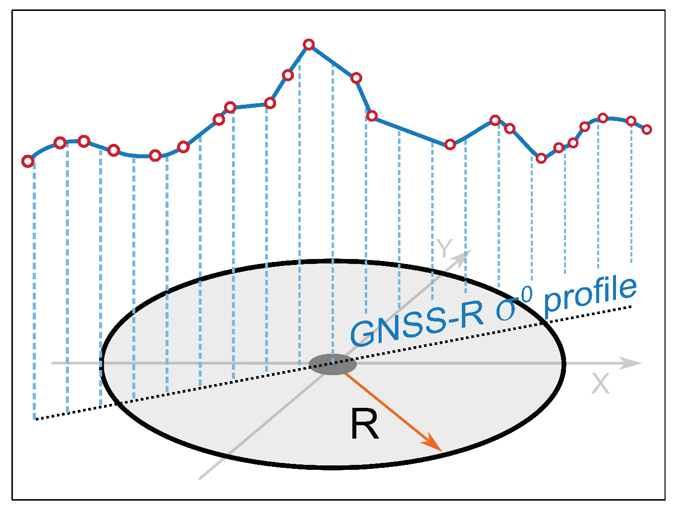
The eddy trajectory atlas detects an eddy as the outermost closed-contour of Sea Level Anomaly (SLA) encompassing a single extremum [22]. The area enclosed by the contour of maximum circum-average speed is considered as the eddy radius R. The CYGNSS tracks overpassing the eddy with a maximum distance of $2R$ from the eddy center are collected and transformed into a local coordinate system (Figure 1). The local coordinate system has the origin at the center of the moving eddy with x- and y-axes oriented toward geographical east and north, respectively. Observations marked with a poor quality flag in the CYGNSS dataset (L1, v2.1) and tracks with more than 10% data loss are excluded from the collocated dataset.

The methodology of this study is based on the following steps. First, the signatures in the CYGNSS ${\sigma }^0$ are visually sought. The observed behavior in several cases can be the first evidence on the possibility of an eddy-left signature in the GNSS-R measurements. This examination is followed by statistical analyses to quantitatively characterize the signatures. We investigate the collocated dataset consisting of more than $2.7\times {10}^5$ NBRCS profiles over ≈ 6000 mesoscale eddies. The profiles in the along-track coordinate system are normalized using the radius of each eddy and gridded between $-1.1\times R$ to $+1.1\times R$ (Figure 1).

The visually observed behaviors of the ${\sigma }^0$ profiles show noticeable changes over the central region or the edges of the eddies. These patterns are along with some linear and nonlinear changes in different scales. To extract the main nonlinear anomalies over the center or at the edges of eddies within the profiles, linear and small scales fluctuations of ${\sigma }^0$ should be filtered out. We apply Principal Component Analysis (PCA) [25] to reduce the dimensionality of the dataset while preserving most of the information within the ${\sigma }^0$ profiles. To this end, a data matrix ${\mathbf{X}}_{\mathbf{m}\times \mathbf{n}}$ is formed using n profiles, each of which with m gridded observation points. The profiles are centered by subtracting the mean values. Using Singular Value Decomposition (SVD), the data matrix X can be written as:

$$\mathbf{X}=\mathbf{U}\mathbf{L}{\mathbf{V}}^{\mathbf{T}}$$

(1)

where the columns of $\mathbf{U}$ and $\mathbf{V}$ are the left and right singular vectors, respectively. $\mathbf{L}$ is a diagonal matrix with non-negative elements, the singular values $\lambda$. A proper group of singular values and corresponding singular vectors is selected to reconstruct the data matrix. Columns of the reconstructed matrix contain the filtered ${\sigma }^0$ profiles. Assuming the set $I=\{i,i+1,...,k\}$ whose elements are the indices of the selected group, the reconstructed data matrix, $\widehat{\mathbf{X}}$ is:

$$\widehat{\mathbf{X}}={\mathbf{X}}_{\mathbf{i}}+{\mathbf{X}}_{\mathbf{i}+\mathbf{1}}+...+{\mathbf{X}}_{\mathbf{k}},{\mathbf{X}}_{\mathbf{i}}={\lambda }_i{\mathbf{U}}_{\mathbf{i}}{\mathbf{V}}_{\mathbf{i}}^{\mathbf{T}}$$

(2)

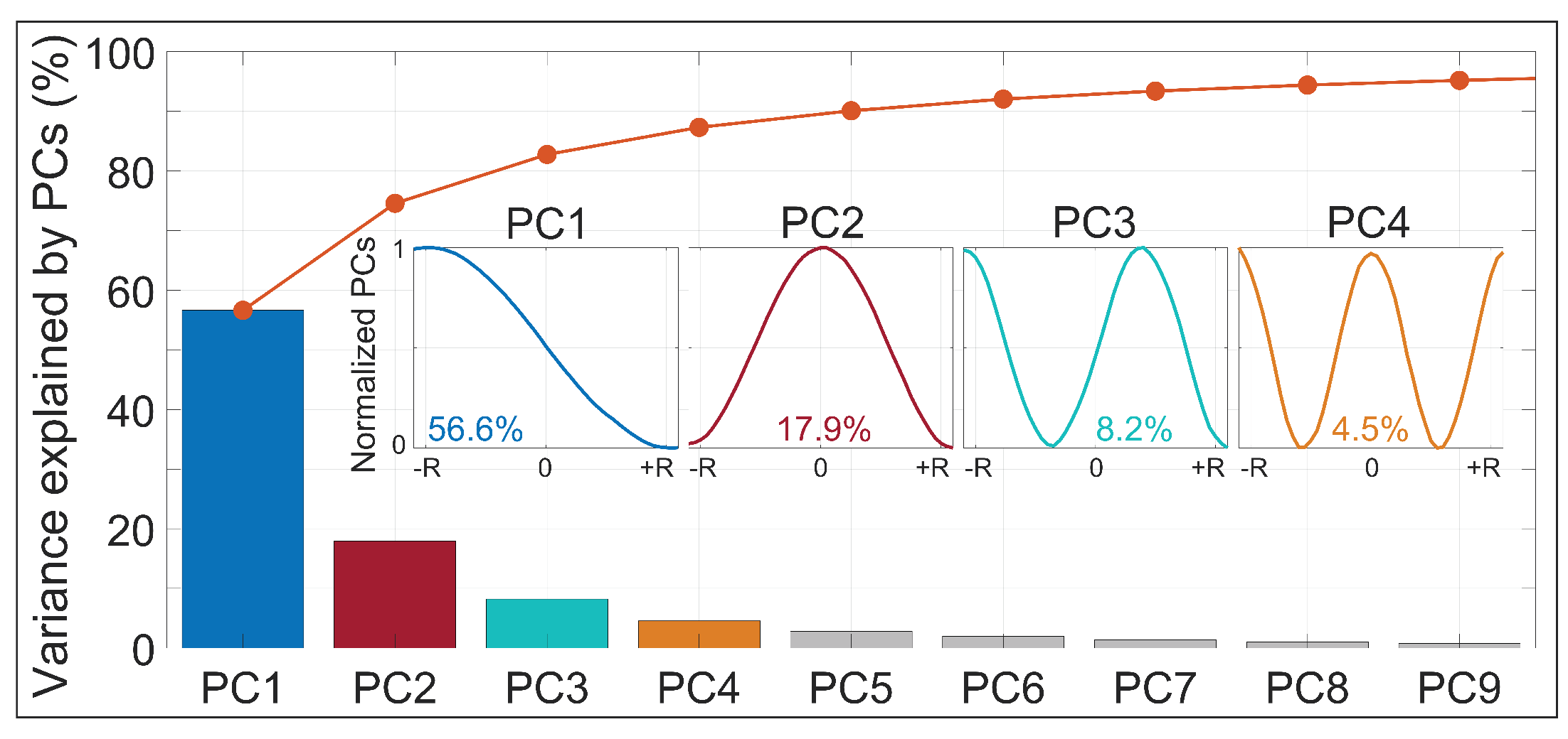
where ${\mathbf{U}}_{\mathbf{i}}$ and ${\mathbf{V}}_{\mathbf{i}}$ are the left and right singular vectors associated with the singular value ${\lambda }_i$. Columns of the matrices ${\mathbf{X}}_{\mathbf{i}}$ represent uncorrelated features of the ${\sigma }^0$ profiles. The quality of each principal component (PC) can be measured by:

$${\Lambda }_i=\frac{{\lambda }_i}{{\sum }_{l=1}^d{\lambda }_l}$$

(3)

where ${\Lambda }_i$ represents the proportion of total variance explained by the principal component i. The parameter d ($d\le min\{m,n\}$) is the number of non-zero singular values.

The investigation is followed seeking the conditions, in which the ${\sigma }^0$ response is more pronounced. To this end, the correlation coefficient between ${\sigma }^0$ and surface sensible heat flux is calculated at different wind speeds. Similarly, the correlation coefficient between ${\sigma }^0$ and the mean turbulent surface stress is obtained in a range of angular differences between the CYGNSS observational track and the turbulent surface stress. The results are presented in the following section.

3. Results and Discussion

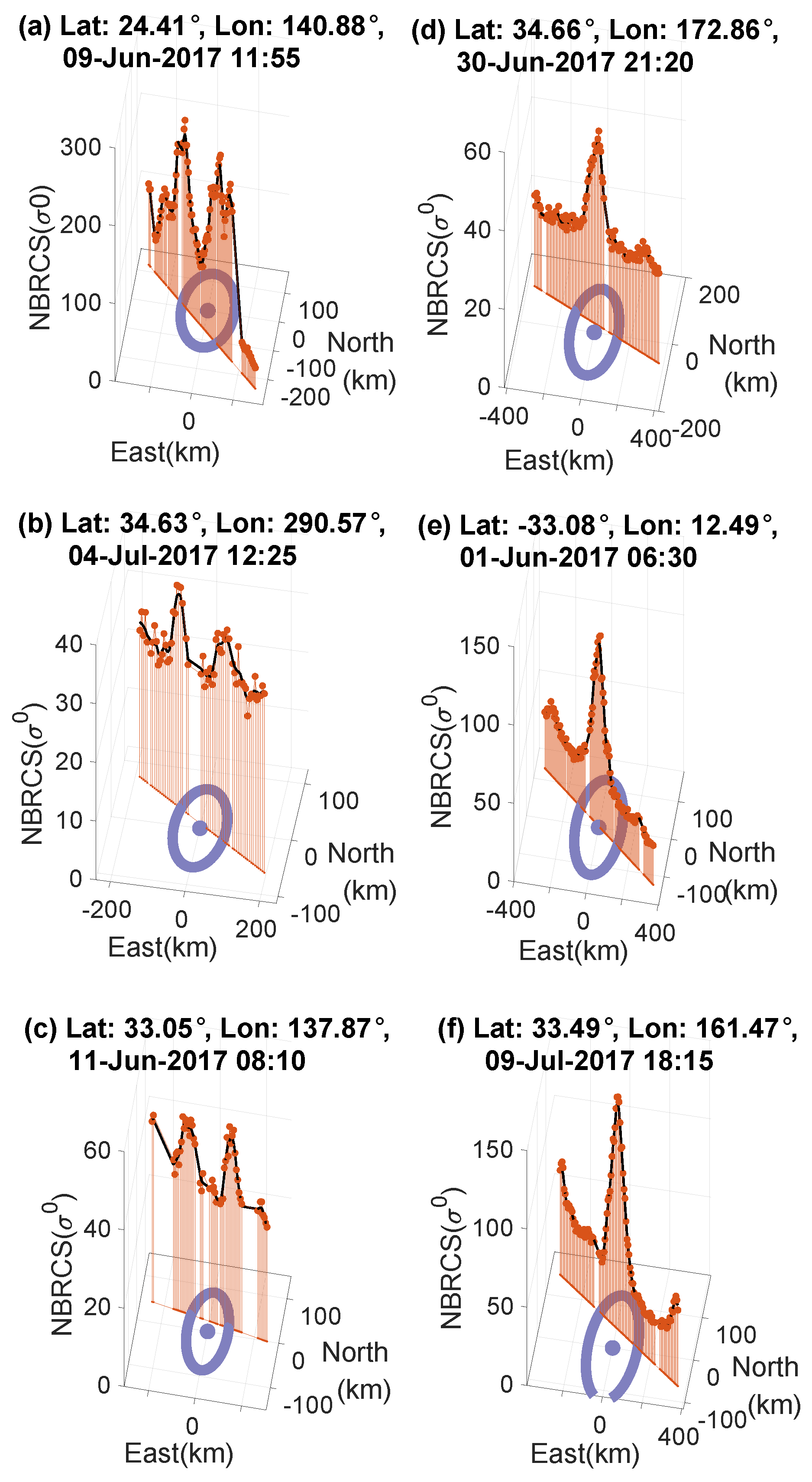
Generally, two prominent anomalies are observed in our investigation as responses of ${\sigma }^0$ to the presence of the eddies: one jump at the eddy center (single-jump behavior) or two jumps at the eddy edges with a lower value at the center (double-jump behavior). Figure 2 demonstrates the double- (a–c) and single-jump (d–f) behaviors in different exemplary cases. The sudden increase in ${\sigma }^0$ is significant enough to be easily discerned in the measurements.

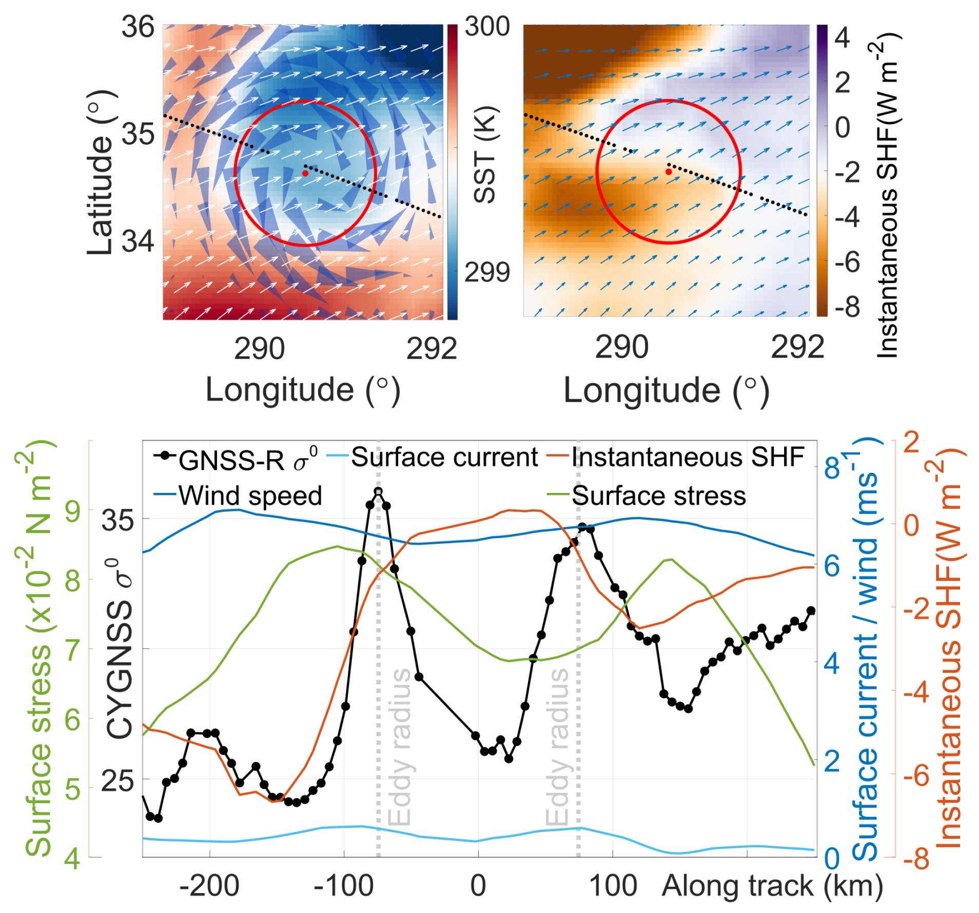
Additional exemplary cases are shown along with the collocated ancillary data in Figure 3, Figure 4 and Figure 5. In Figure 3, clear fluctuations are repeatedly demonstrated over the eddy edges (similar to Figure 2a–c). Once the track enters the eddy-affected area, ${\sigma }^0$ increases significantly and then drops quickly at the center followed by another jump once the track leaves the eddy.

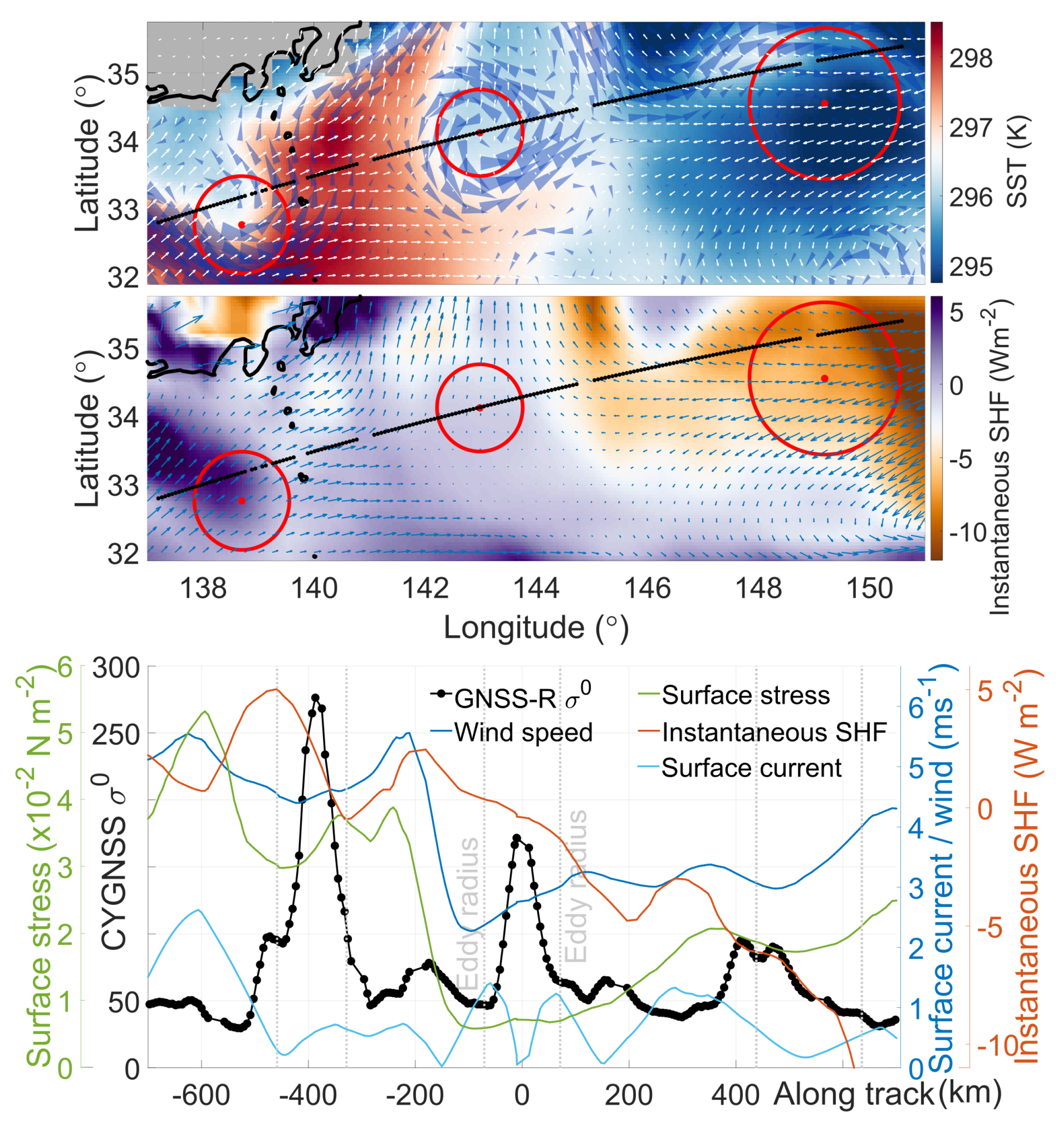
Figure 4 shows a CYGNSS track which is long enough to overpass three cyclonic eddies. The ${\sigma }^0$ behaves similarly to Figure 2a–c and Figure 3. The track does not cross the first eddy center. This causes an increase in the value of ${\sigma }^0$ when it passes the eddy outer lying area. A remarkable fact is that ${\sigma }^0$ remains almost at the same level moving over the eddy edges and again drops to lower values once it leaves the affected region. Reaching the second eddy, the track sweeps also the areas close to the eddy center and ${\sigma }^0$ responds with a lower value at the center and two considerable increases at the edges. The behavior of ${\sigma }^0$ is similar over the third eddy, however, the peaks stand at lower values.

Figure 5 shows another CYGNSS track overpassing three eddies. Similar to Figure 2d–f, ${\sigma }^0$ shows a single peak at the center. The track enters the core region with a sudden increase in ${\sigma }^0$ which again drops to its initial level once the track moves off the center. Similar behavior of ${\sigma }^0$ is observed reaching the central region of the second and third eddies.

Figure 6 shows the PCA results where the first nine principal components of the dataset preserve more than 95% of the statistical information in the dataset. The PCs represent low to high-fluctuating patterns within the profiles. The first PC mainly reflects the overall linear trend of the ${\sigma }^0$ profile. The other PCs capture the remaining non-linear variations of the profiles over the eddies. We reconstruct the profiles using the eight components PC2-PC9 and calculate the correlation coefficient of each reconstructed profile with synthetic templates of the two observed patterns. Since the peaks over the edges or at the center of the eddies could be slightly displaced from the exact expected location, we consider up to $\pm 0.1\times R$ lag for the calculation of the correlation.

The analysis reveals that about 12.7% (15.9%) of profiles demonstrate a correlation coefficient of 0.7 or more with the single (double) peak template. We also carried out the same statistical analysis over a new set of profiles collected regardless of the presence of eddies. In a reverse approach, the profiles demonstrating a high correlation with the templates (≥ 0.7) are investigated. About 45% of these profiles are either located on the eddies (according to the Aviso’s trajectory atlas) or show a high correlation (≥ 0.7) with the surface current.

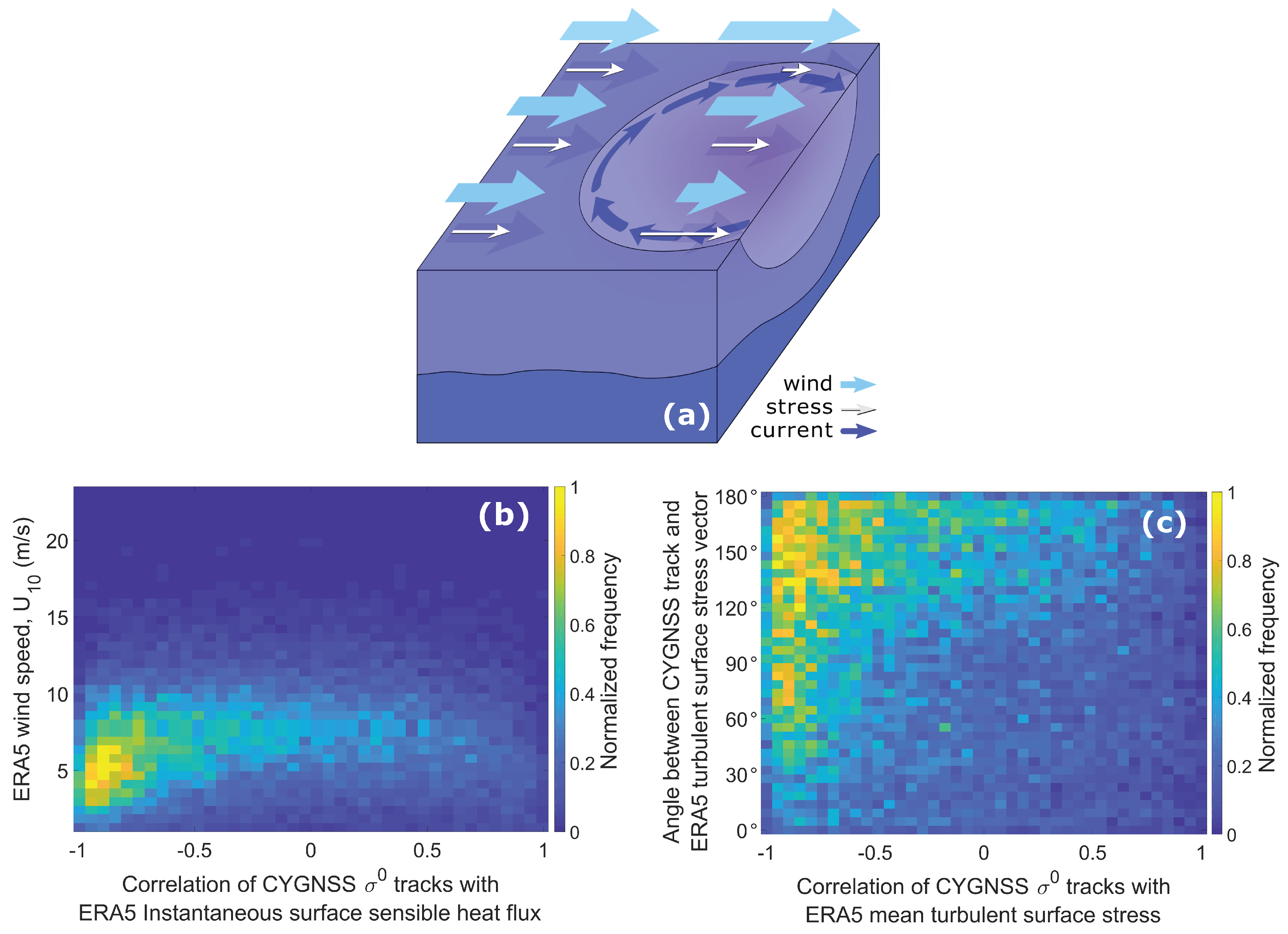
Results of the next statistical analysis over the collocated dataset reveal a strong negative correlation of CYGNSS ${\sigma }^0$ observations with both SHF and surface stress under certain conditions. Figure 7 provides insights into the favorable conditions, in which CYGNSS is more likely to sense surface stress and SHF over the eddies.

Figure 7a illustrates a simplified model of changing surface stress due to the interaction between the eddy surface current and wind speed. In Figure 7b, the behavior of ${\sigma }^0$ is highly correlated with SHF over the eddies at wind speeds between ≈3 m/s and 7 m/s, where the values of the correlation coefficients are mainly between −0.8 to −0.95. According to the theory, at high enough wind speed ($\approx >$ 5 m/s), the surface parameter that controls the intensity of GNSS reflections from the ocean surface, or ${\sigma }^0$, is the low-pass mean square slope, $MS{S}_{LP}$, of the ocean surface [26]. It is determined by the part of the wave slope spectrum that resides at wavenumbers smaller than $k_{*}=kcos{\theta }_{inc}/3$ where ${\theta }_{inc}$ is an incidence angle and k is the wavenumber $(2\pi /\lambda )$ of the L-band GNSS signal [27]. The ${\sigma }^0$ is inversely proportional to $MS{S}_{LP}$. The largest contribution to the $MS{S}_{LP}$ originates from the short-wave portion of the spectrum near $k_{*}$. From classic works of [28,29], it is known that there are two main mechanisms affecting that part of the wave spectrum: the varying wind surface stress and interaction of short waves with the current gradients. At low enough wind speed, the scattering of GNSS signals does not follow a pure quasi-specular scattering and there is a coherent scattering component that tends the mechanism to a higher-order Bragg scattering, driven by Rayleigh parameter [30]. Rayleigh parameter is proportional to waves at any wavenumbers. So, at this regime of wind speed, GNSS-R measurements could be more sensitive to surface state, even to small-scale roughness modifications [12]. Figure 7c shows the impact associated with the angular difference of CYGNSS tracks and surface stress field direction. The direction of the CYGNSS track with respect to the surface stress vector can increase the sensitivity of ${\sigma }^0$ to surface stress anomalies within the eddies. This means the GNSS-R measurements are highly likely to sense the stress field with a direction against the moving GNSS-R specular points. It can be also seen that for the absolute angular distances in the range of about 60 to 180 degrees the wind stress would be more pronounced in the CYGNSS measurements.

Atmospheric boundary layer change associated with the eddy-induced SST anomalies results in a varying wind field [31]. The modified local surface wind influenced by marine boundary layer dynamics [32,33] can partially explain the GNSS-R ${\sigma }^0$ patterns. The enhanced local wind over the warm core of the eddy can lead to the abrupt change in the GNSS-R ${\sigma }^0$ values. Since the improvement in the weather and climate projections require detailed observations and understanding of warm eddy-atmosphere interactions [34], this possible promising contribution by the GNSS-R technique should be investigated.

The first cold-core eddy shown in Figure 5 can cause a strong dampening of wind intensity due to downward transport of wind momentum, decelerating local surface wind. The sharp peak of GNSS-R ${\sigma }^0$ resides at the core region of the eddy where the SST has a lower value. This deceleration could also happen when a tropical cyclone reaches a strong cold-core eddy. Such eddies can broaden the eye size of the storm during its passage and reduce its intensity [35]. For instance, an unforeseen rapid weakening was demonstrated when the category 4 hurricane Kenneth passed over a cold-core eddy on 19–20 September 2005 [36].

The discussed air-sea interactions over the eddies could explain the response of GNSS-R observations to SHF at the ocean-atmosphere interface through the modified surface stress. In Figure 3, a local minimum of ERA5 surface stress values takes place almost over the core region of the eddy. The peaks of the stress values approximately reside over the rotating current of the eddy. The impact of the surface stress on the profile of CYGNSS ${\sigma }^0$ is evident where sudden fluctuations are seen over the edges and in the core. Larger SHF values with negative sign, i.e. upward direction of the flux, are well synchronized with two ${\sigma }^0$ minima at -150 and 150 km along with track coordinates.

In Figure 4, the most prominent change in the ${\sigma }^0$ profile can be seen over the middle eddy. The possible signature of this eddy could be explained by a high value of stress approximately at the eddy center where an increment of upward SHF is observed. The ERA5 could be subjected to deficiencies in resolving local sudden changes and It seems that it does not reveal the same level of details over the left eddy as those provided by the CYGNSS measurements. The behavior of ${\sigma }^0$ over the right eddy in this figure can be described by the expected behavior of ${\sigma }^0$ at very low wind speeds. According to [37], at very low wind speeds (< 2.5 m/s), the bistatic radar cross section is directly proportional to the roughness (unlike the inverse correlation at higher wind speeds). Therefore, the clear correspondence between the magnitude of upward SHF and wind speed over this eddy closely matches the similar pattern in ${\sigma }^0$ while the wind speed values are mainly below 2 m/s.

The surface current associated with eddies is another factor that can affect surface stress. Considering surface stress as a function of wind and ignoring the surface current in the oceanic numerical modeling, can result in the overestimation of the total energy input of wind to the ocean [38]. Wind stress ($\tau$) can be calculated as [39]:

$$\tau ={\rho }_a{C}_D\left(W-U\right)\left|W-U\right|$$

(4)

where ${\rho }_a$ is the density of the air, $C_D$ is the drag coefficient, and W and U are the wind and surface current, respectively.

The behavior of ${\sigma }^0$ in Figure 5 can be partially attributed to the modified surface stress at the eddy currents. Eddy-induced current can amplify or decrease the wind stress (Figure 7a) or alter its direction which can in turn change the level of ${\sigma }^0$ sensitivity to surface stress. Over the left eddy in Figure 5, the similar directional orientation of the CYGNSS track with respect to the surface stress field can lead to the weaker impact of stress on the ${\sigma }^0$ values (see Figure 7c). Interaction of eddy-induced current with surface stress can increase the ${\sigma }^0$ sensitivity over the edges resulting in lower ${\sigma }^0$ values. Therefore, the vanishing current at the core region would lead to the less pronounced impact of stress on ${\sigma }^0$. Although the stress field over the middle eddy is not as strong, the angular difference of the CYGNSS track with the stress field intensifies the impact. The strong current velocity on the edges enhances the stress on the left side and decreases the stress on the right side of the eddy (see Figure 7a), resulting slightly higher ${\sigma }^0$ values on the right edge compared to the left edge. The low magnitude of SHF over this cold-core eddy together with almost zero current velocity at the center cause a sudden peak in the ${\sigma }^0$ value. The higher SHF magnitudes and stress values between the two eddies keep the ${\sigma }^0$ values at a lower level.

It is worth mentioning that concentrated biogenic films from natural life in the ocean can potentially play a role in the power of reflected GNSS-R signals. The turbulence associated with the eddies brings the natural biogenic surfactants released from plankton and fishes to the surface, where the concentration of the surfactant molecules can generate a surface tension. This phenomenon could inhibit the development of Bragg waves [40]. Such areas are discerned as dark regions in the synthetic aperture radar images since the signal is mainly forward scattered rather than being backscattered. In a bistatic forward scattering configuration, the wide-enough smoothed regions can increase the power of GNSS signals after reflection from the ocean. Therefore, a dramatic increase in ${\sigma }^0$ over these regions can be expected. The characterization of biogenic surfactants’ role in the signal forward scattering is recommended for future studies.

4. Conclusions

In this study, it is shown that spaceborne GNSS-R measurements can respond to the existence of eddies. Different characteristics of eddies can impact the local wind as well as surface stress which can, in turn, affect GNSS-R measurements. The normalized bistatic radar cross section (NBRCS) exhibits a clear inverse correlation with surface heat flux and surface stress under certain conditions. Nevertheless, characterization of the observed signatures requires further study considering other potential factors such as the effect of biogenic surfactants and the eddy-induced currents in the surface stress and ocean state. Many factors produce NBRCS changes. The complexity of oceanic and atmospheric mechanisms controlling the GNSS scattering demands further sophisticated analyses in future studies. There are still open questions such as the conditions of occurrences or the measurements specific behaviors over cyclonic or anticyclonic eddies. This study initiates the development of the novel GNSS-R technique for studying ocean mesoscale eddies, the feasibility of which has been demonstrated for the first time.