Abstract
Site-dependent effects are now the key factors that restrict the high accuracy applications of Global Navigation Satellite System (GNSS) technology, such as deformation monitoring. To reduce the effects of non-line-of-sight (NLOS) signal and multipath, methods and models applied to both of the function model and stochastic model of least-squares (LS) have been proposed. However, the existing methods and models may not be convenient to use and not be appropriate to all GNSS satellites. In this study, the SNR features of GPS and GLONASS are analyzed first, and a refined SNR based stochastic model is proposed, in which the links between carrier phase precision and SNR observation have been reasonably established. Compared with the existing models, the refined model in this paper could be used in real-time and the carrier phase precision could be reasonably shown with the SNR data. More importantly, it is applicable to all GNSS satellite systems. Based on this model, the site observation environment can be assessed in advance to show the obstruction area. With a bridge deformation monitoring platform, the performance of this model was tested in the aspect of integer ambiguity resolution and data processing. The results show that, compared with the existing stochastic models, this model could have the highest integer ambiguity resolution success rate and the lowest noise level in the data processing time series with obvious obstruction beside the site.
1. Introduction
Global Navigation Satellite Systems (GNSS) are now gradually recognized as an essential tool in every aspect of geodesy and geodynamics. Especially in the application of high precision deformation monitoring, the relative double differential positioning technology with short baselines is widely applied, due to the advantages of eliminating satellite orbits errors, receiver and satellite clock offsets, and of reducing ionosphere and troposphere delays. Furthermore, it is also a relatively easy way to process the data compared with the long baseline data processing. The benefits make the short baseline double difference (DD) mode to be an ideal method in the engineering application. Generally, in an open viewing environment, the precision of millimeter level in horizontal directions and centimeter to sub-centimeter level in vertical component could be achieved regardless of a static or kinematic mode with multiple GNSS (Multi-GNSS) phase observations [1,2,3,4]. However, in the deformation monitoring application, the monitoring stations are mounted on the targeted objects. GNSS signals are inevitably sheltered or reflected by obstructions, such as bridge towers, cables and vehicles on a bridge, and each station has a specific observation situation [5,6]. From the literature review, we know that the signal obstruction can mainly cause three essential problems. They are, (1) multipath effects from signal reflection, (2) signal diffractions and (3) the satellite geometry strength reduction. The paper calls these problems uniformly as site-dependent effects [6,7]. Since the site-dependent effect is related to the observation environment at each station, it cannot be eliminated by double differencing so as to be an unresolved problem in the short baseline data processing [7,8].
The GNSS carrier-phase observations are generally resolved by means of least-squares (LS) method. However, only if both of the function model and stochastic model are realistic, can the unknown parameters be precisely estimated [9,10,11]. In the data processing, the function model describes the mathematical relationship between the unknown parameters and the GNSS phase observations. The aim of stochastic model is to describe the a priori statistical properties of the observations with an appropriately defined variance-covariance matrix [7,12]. As for the site-dependent error, a variety of eliminating methods have been proposed in the aspects of functional and stochastic models by many studies.
In the functional model, the methods can be divided into three categories. Firstly, it will be the spatial or temporal repeatability-based sidereal filters. The constellations of GNSS satellites are repeated, and the repeat periods are differed from different GNSS systems. The temporal sidereal filter is based on the repeat time, which could be calculated in advance, and generates the multipath correction model for real-time GNSS data processing [13,14,15,16,17,18,19]. In the multipath modelling process, Wavelet [20,21,22], Adaptive filter [23] and Vondrak filter [24] could be applied. Alternatively, the spatial repeatability-based model is based on the fact that the multipath relies on the orbital position in the sky [8,25,26]. The multipath model could be generated as the function of satellite elevation and azimuth angle. Secondly, the Signal-to-Noise Ratio (SNR) data could be applied to model the multipath effects. SNR is a measurement in GNSS raw data to express the signal power [27]. The reflection and diffraction signals from an obstruction could have a low or high frequency fluctuation in the SNR time series. Thus, the multipath or diffraction signals can be extracted from SNR time series with spectrum analyzing methods [28,29]. Similarly, a spatial or temporal model can also be built. In the third category, three-dimensional (3D) maps [30,31], Ray-Tracing technology [32], a terrestrial laser scanner (TLS) or SNR data [7,33,34,35,36] could be used to recognize and exclude the non-line-of-sight signals (NLOS). All the methods stated here may have a good performance in a specific application. However, they may have drawbacks, such as complex implementations, inadequate resolutions and inapplicability to routine surveying tasks.
As for the stochastic model related method, the SNR measurements are often used to weight the one-way carrier phase observations. As previously mentioned, the SNR measurements can express the signal quality. The SNR based stochastic model will be more reasonable than the elevation-dependent weighting model. Brunner et al., Wieser and Brunner and Luo et al. have all explored the SNR based models [12,27,37]. The experiments confirmed that these methods can effectively reduce the multipath effect, improve the ambiguity resolution (AR) success rate and enhance the repeatability of site coordinates [9,12,27]. However, these studies only focus on the functional relationship between the satellite elevation and SNR data. The relationship between the precision of raw observation and SNR data is rarely studied. Meanwhile, more GNSS systems, such as GLObalnaya NAvigazionnaya Sputniovaya Sistema (GLONASS), BeiDou Navigation Satellite System (BDS) and Galileo, are available now to provide positioning, navigation and timing (PNT) services. The GPS related formulates may not be feasible to other systems.
Under such cases, a refined SNR based stochastic model, which is applicable to any GNSS system, is proposed to deal with the site-specific errors. At the beginning, the relationship between SNR time series of GPS and GLONASS with elevation and precision of carrier phase is studied based on the GeoSHM (GNSS and Earth Observation for Structural Health Monitoring of Bridges) platform. Then, the stochastic modelling method is introduced. In the end, the performance of the new SNR based stochastic model used in observation environment assessment and in ambiguity resolution and positioning is analyzed.
In Section 2, the experiment data used in the paper from the GeoSHM platform is introduced first for the beneficial of understanding the refined model and the following experiments. In Section 3, we compare and discuss the features of GPS and GLONASS SNR data and describe the method of refining the SNR based stochastic model. In Section 4, several experiments are carried out to show the effectiveness of the refined model in observation evaluation and data processing. A discussion will be shown in Section 5, and Section 6 gives the conclusions about this paper.
2. Data Description
The experiment data are from GeoSHM, which is a project hosted by the University of Nottingham, Ubipos UK Ltd. and other partners under the sponsorship from European Space Agency (ESA) [2]. The aim of the project is to study and develop a stable and reliable bridge health monitoring system with the integration of multiple sensors, such as GNSS, Inertial Navigation System (INS) and Earth Observation (EO), and realize the real time monitoring and assessment of bridges. The layout of the system is shown in Figure 1. Up to date, the Feasibility Study and Demonstration development stages have completed, and the system has been used in Forth Road Bridge in the UK and two Yangtze River bridges in China.
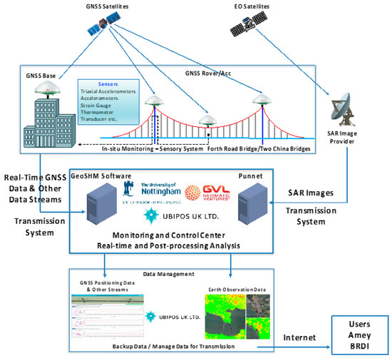
Figure 1.
Layout of the GeoSHM system.
The data source used in this paper is collected from the GeoSHM system, including the receiver testing bed on the roof of the Nottingham Geospatial Building on the Jubilee Campus of the University of Nottingham, UK and the real-life bridge monitoring on the Forth Road Bridge (FRB) in Scotland, UK.
The stations’ setup of receiver testing bed is shown in Figure 2. A Leica GM30 receiver is set as a reference station (SHM7). Two Leica GM30 (SHM5, SHM6) and two PANDA TI4100 (SHM8, SHM9) receivers are connected to one antenna as a monitoring station. More detailed information can be seen in Xi et al. [38]. Xi et al. have used the data set to estimate the precision of raw phase observations and refined the elevation dependent stochastic model. In this paper, as a follow-up research, the features of SNR data of GPS and GLONASS, and the functional relationship between SNR and phase precision is further studied in Section 3. Only the data collected from LEICA receivers will be used in this paper and the receivers were set to collect GPS and GLONASS data. The data were collected for two days (48 h) with a sampling interval of 1 s. The cutoff elevation was set to 10°.
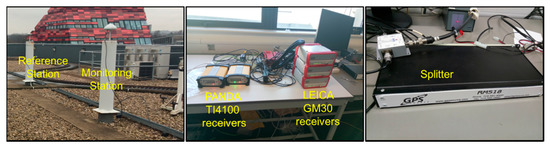
Figure 2.
Receiver testing bed of GeoSHM system.
On the Forth Road Bridge, four stations in the GeoSHM system will be selected to do the test. Among the stations, SHM1 is the reference station, which is mounted at the roof of the bridge control room. SHM2 and SHM3 are two monitoring stations on both sides of the middle span, and SHM4 is the one sitting on the top of the southwest tower of the Forth Road Bridge (FRB) [2]. All stations are equipped with a LEICA GM30 receiver and a LEIAR 10 antenna (same with the receiver testing bed). Sampling rate is set to 10 Hz. Figure 3 depicts the landscape of the FRB, the locations of stations on the FRB and the baseline lengths, and the observation environment of the stations.
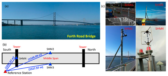
Figure 3.
(a) The landscape of FRB, (b) antenna setting-ups on the Forth Road Bridge and the baseline lengths and (c) the observation environment of the stations.
3. The Refined SNR Based Stochastic Modelling Method
3.1. GPS/GLONASS SNR Measurements Analysis
Before the stochastic modelling, features of the SNR measurement of GPS and GLONASS should be analyzed first and the regularity with the variance of satellite elevation and phase precision should also be tested.
Figure 4 shows the averaged GPS and GLONASS SNR measurements in 22 January 2017. One can observe that all the GPS satellites share a same feature that the L1 SNR is 5 to 10 dB higher than the L2 counterpart. The differences between satellites are within 8 dB. For GLONASS satellites, except for several satellites whose L2 SNR data is obviously lower than the L1, the two frequencies show the nearly same pattern of the averaged SNR value. However, a large distinction may be seen between different satellites.
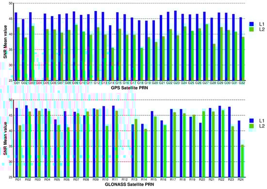
Figure 4.
Mean value of GPS and GLONASS SNR measurements in site SHM5 for 22 January 2017 (DOY = 22).
Figure 5 and Figure 6 are the SNR time series versus the variation of satellite elevation for site SHM5 and SHM7. In the figures, different colors denote the individual satellites, and every dot indicates the averaged SNR value within one degree of elevation. It can be seen that, except for some slightly detailed differences, two stations have a similar feature in the SNR time series. Therefore, for the same type of GNSS receivers, they should have almost the same data collection performance under a similar observation condition.
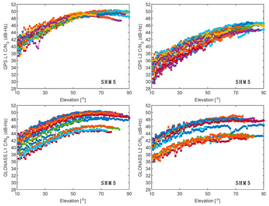
Figure 5.
GPS and GLONASS SNR average value within one elevation versus elevations at site SHM5.
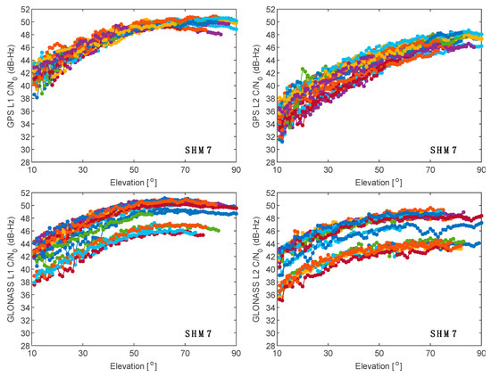
Figure 6.
GPS and GLONASS SNR average value within one elevation versus elevations at site SHM7.
In addition, it is interesting that GPS satellites have a coincident fluctuation feature; however, different patterns were separately shown for GLONASS satellites in dual-frequency signals. However, their elevation dependent features were similar. Then, we gave the precision of carrier phase observations with the variance of elevation in Figure 7. The precision estimation approach is shown in Xi et al. 2018b [38]. We can observe from Figure 7 that the GPS and GLONASS phase observation precision is elevation dependent and no obvious different patterns are shown in GLONASS phase precision. Therefore, we may conclude that the absolute SNR value may not be appropriate to give weight for the one-way observation directly with a formula as Hartinger and Brunner (1999) [37].
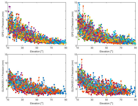
Figure 7.
Phase precision estimation of every one-degree elevation for GPS and GLONASS.
3.2. The Refined SNR Based Stochastic Model
As previously mentioned, the absolute SNR value may not be properly used to weight GNSS phase observations, and the SNR time series is elevation dependent. Hence, we firstly normalize the SNR observations to range from zero to one. This process can eliminate the different patterns phenomenon in GLONASS system. Although there are no different patterns in GPS, the normalization approach is also appropriate for GPS. The normalization process can be written as:
where is the normalized SNR value; is the measured SNR value; and are the minimum and maximum value, respectively, in Figure 5 and Figure 6. The normalized SNR value for SHM5 is shown in Figure 8.
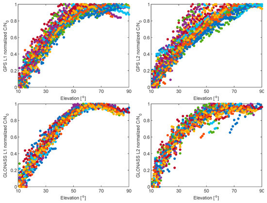
Figure 8.
The normalized SNR time series for SHM5.
From the figure, the normalized SNR tend to approach to the maximum value at around 50 degree of elevation. The values lower than 50 would have a liner trend feature. As for the GLONASS system, the normalized dual-frequency SNR data from different satellites gather together and toward to a similar trend. This demonstrates that different GLONASS satellites’ antenna gain against the satellite elevation may be different from each other, however, the variation of SNR along with the elevation variation tend to have a same pattern.
We also calculate the mean value of normalized SNR from all GPS and GLONASS satellites in the dual-frequency band (Figure 9). The sample of elevation is one degree. Under such cases, GPS and GLONASS have a same SNR variation trend against the elevation. However, when the elevation is in the range of 40 to 70, the averaged normalized SNR of GPS L2 is slightly lower than other satellite signals.
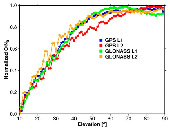
Figure 9.
The mean value of normalized SNR of all satellites for one elevation in dual-frequency GPS and GLONASS.
As proposed by Xi et al., Li et al. (2015) [10,38], the elevation-dependent precision of GNSS carrier phase observations can be fitted with an exponential or sinusoidal type of predefined function of elevation. Similar to this theory, the exponential type function was applied to fit the normalized SNR:
where is the fitted normalized SNR value and , and are the fitting parameters. Figure 10 shows the normalized SNR data and their fitted models. In the figure, the carrier phase precision estimation is also shown to illustrate the links between SNR data and precision estimations. It shows that the exponential function model fits the time series well. With the increase of elevation, the normalized SNR grows up steady and the observation precision increases gradually, and the two lines intersect at around 25° for all types of observations. Furthermore, an inversely proportional relationship can be observed from these figures. Therefore, the paper treats elevation as an index to align the normalized SNR data (as x-axis) and the observation precisions (as y-axis), in which the estimates (blue points) and modelling results (green points) are displayed (in Figure 11).
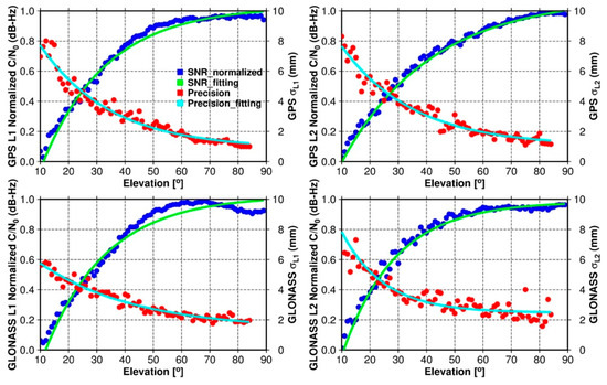
Figure 10.
The estimated elevation-dependent precisions in Xi et al. and normalized SNR data, and their modelling with the exponential type predefined models.
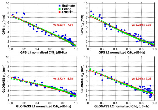
Figure 11.
The functional relationship between normalized SNR data and the precision of phase observations.
One can clearly observe a linear relation between the normalized SNR data and the precision of phase observations in dual-frequency observations of GPS and GLONASS. Then, the coefficients are resolved with a linear least-squares method, and the fitting model and the linear equations are also shown in Figure 11. In this case, the linear model shown in Figure 11 could be used as a refined SNR-based stochastic model to weight the phase observations.
3.3. The Flow Chart of the Refined SNR Based Stochastic Model and the Application Strategy
As previously mentioned, the precision of phase observations and the normalized SNR data should be linked in advance. The GNSS carrier phase precision estimation and the elevation related model can be built with the approach proposed by Xi et al. [38]. The interval is in the unit of one degree. For the SNR sub-step, we need to record and average the SNR observations each elevation angle of 1°, and obtain the maximum and minimum values and (Figure 5 and Figure 6). Then, the averaged SNR observations of each elevation angle of 1° can be normalized with Equation (1). Therefore, the elevation related feature of the normalized SNR can be obtained (Figure 8). Finally, we treat elevations as an index to align the normalized SNR data (as x-axis) and the observation precisions (as y-axis) (Figure 10), and a linear least-squares method is applied to fit the model (Figure 11). It should be noted that the model is only applicable for the same type of receivers.
In the GNSS data processing, when we get the SNR observations, it should be normalized by Equation (1) with the recorded and . Then, the phase observation precision can be obtained by substituting the normalized SNR into the linear stochastic model. If the practical SNR is larger than , the highest precision will be given. However, if the practical SNR is lower than , the output precision may be used, or the observation of this satellite would be moved out directly due to the unreliable quality of this observation. Therefore, we can understand that, if the pre-prepared model is established for a specialized receiver, it can be used in real-time mode of data processing.
4. Experiments and Results
4.1. Assessment of Station Observation Environment
Before the data processing, SNR observations are often used to assess the observation environment of stations. Figure 12 shows a one-day SNR related sky-plot of GPS and GLONASS satellites at station SHM5 (22 January 2017). The color demonstrates the raw SNR observations from a GNSS receiver. It is clearly shown that, for the L1 phase observation, the SNR is elevation related, and the value is larger than 46 dB-Hz for the elevation higher than 45°. Then, it begins to reduce with the declining elevation. However, several satellites have a lower SNR value for the whole session. For the L2 phase observation, the SNR value is clearly lower than L1. Though the elevation dependent feature is noticeable, it shows a large difference between different satellites. In this case, it is difficult to distinguish the orientations of the disturbed signals.
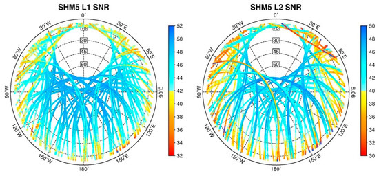
Figure 12.
SNR-based sky-plot of GPS and GLONASS at SHM5.
Figure 13 shows the phase precision related sky-plot of GPS and GLONASS at SHM5. The phase precision is the output of the linear stochastic model previously built when the observed SNR value shown in Figure 12 is as the input. From Figure 13, the elevation dependent feature of the phase precision can be clearly noticed no matter for L1 and L2 observations. Mostly, the precision is better than 6 mm for the open viewing observation environment. Only the observations whose elevations are lower as to 10° show a low precision, and the numbered 1-4 cycles show the orientations with a lower precision.
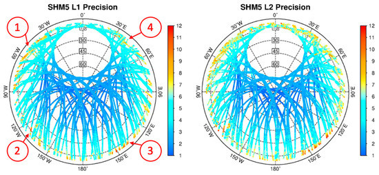
Figure 13.
Carrier phase precision (mm) related sky-plot of GPS and GLONASS at SHM5.
Figure 14 gives the realistic observation condition for SHM5. It shows the potential obstructions whose heights are slightly higher than the station, which has been numbered 1–4. Compared with Figure 13, the precision decreases in Figure 13 are basically caused by the obstructions. Especially for the hollowed-out architecture in position 2, GNSS signals passing through it can cause serious signal diffraction, which may reduce the phase precision to lower than 10 mm.
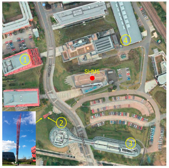
Figure 14.
The observation environment for SHM5.
4.2. Bridge Monitoring Experiment Analysis
An experiment is carried out on the Forth Road Bridge in Scotland. The data were collected on 6 January 2018. Based on the SNR observation data, the refined SNR-based stochastic model built previously is applied to plot the precision sky-plot in Figure 15. Compared with Figure 13, the L1 precision sky-plot of stations on the bridge are mostly same as SHM5 in Figure 13. However, it is significantly worse for the L2 precisions than for SHM5. This may be because the L2 signal is easily influenced by the multipath effect from water surface or obstructions. In addition, from the precision sky-plot, one can easily identify the obstructed orientations for the station. It shows that the data of east side of SHM1 and southeast side of SHM4 is contaminated by the multipath or obstructions. The precision of L1 signal is around 9–10 mm, which is significantly lower than the regular quality ones for 4–5 mm. Therefore, if the elevation dependent stochastic model was applied, the weight of GNSS observations could not be reasonably given, which may have an adverse effect for the ambiguity resolution and positioning.
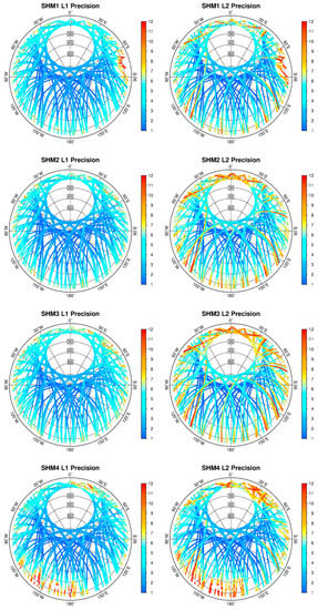
Figure 15.
Precision sky-plots of GeoSHM stations.
4.3. Ambiguity Resolution Performance Analysis
In this section, we process the baseline SHM1-SHM2 and SHM1-SHM4 of GPS and GLONASS data to analyze the single epoch ambiguity resolution performance in a real-time mode. Due to that SHM2 and SHM3 share a similar observation condition, the results in SHM3 will not be shown in the following statements. The data processing software was home-developed and supports integration processing of GPS/GLONASS data. The processing configurations and strategies can be found in Xi et al. [38]. For the comparing purpose, four observation weighting schemes will be applied in the data processing are shown in Table 1

Table 1.
Four weighting models and formulas.
In Table 1, is the standard deviation of the undifferenced carrier phase observations. denotes the frequency number ( = 1, 2). The EEM model is the widely used empirical elevation model in GNSS data processing [39,40,41]. and are the parameters and is the elevation. The ERM is the model established in Xi et al. [38], which is a refined elevation model established for the GeoSHM project. The parameters of ERM have the same meaning as Equation (2) and the estimations can also be found in Xi et al. [38]. The SEM model is the first SNR-based stochastic model proposed by Brunner et al. (1997) [27], and the parameter is from Dai et al. (1998) [42]. The SRM model is the refined SNR based stochastic model proposed in this paper and the coefficients and are shown in Figure 11. indicates the GPS (G) or GLONASS (R), and indicates the PRN number of GPS ( = 1~32) and GLONASS ( = 1~24). and represent the raw SNR observations and the normalized ones, respectively. Since the sampling rate is high, we applied the TEQC software to resample the GNSS data into 15 s for each station.
In the data processing procedure, the ambiguity parameters of L1 and L2 will be reformed into wide-lane (WL) ambiguity and be searched with the LAMBDA (Least-squares ambiguity decorrelation adjustment) method first. If the WL ambiguity is successfully fixed, the L1 ambiguity parameter (NL) then will be searched by LAMBDA. From the long-term data processing experience, the ratio value could be set to 1.8 for the validation.
Figure 16 shows the single epoch WL ambiguity resolution success rate with different ratio values for the schemes listed in Table 1. Firstly, it should be noted that the ambiguities cannot be fixed in the whole section for the SEM model. This is most likely because the parameters of SEM model are not appropriate for GLONASS data. Thus, only EEM, ERM and SRM results are shown in Figure 16. From the figure, the SRM model always shows a better performance than the ERM and EEM model for the two baselines. Due to the better observation environment of SHM2, the ASR (Ambiguity Successful-fixed Rate) can even reach up to 100% when the ratio value is set to 2, and it can still achieve to over 70% at the ratio of 6. Compared with the ERM model, the SRM model has only a small advantage. However, for SHM4, when the obvious obstructions exist around the station, the SRM model shows a much better result compared with EEM and ERM models. When the ratio value is set to 2, the ASR can still reach to 95%, while the ASR decreases dramatically when increasing the ratio value. In this case, it is found that the refined elevation model and the SNR-based stochastic model would have a same performance in ambiguity resolution for the open viewing stations. However, the refined SNR-based model is superior under the obstructed environment.
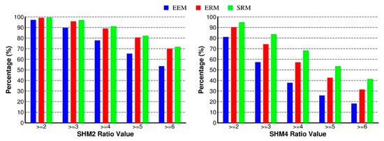
Figure 16.
Success rate of WL ambiguity resolution for schemes of EEM, ERM and SRM.
After fixing the WL ambiguity, Table 2 shows the ASR of NL ambiguity resolution when the ratio is set to 2. The three models show the same performance on NL ambiguity resolution at each station. However, the ASR of SHM2 is much better than that of SHM4. This is still because of the less obstructions around SHM2.
Table 2.
ASR of Narrow-lane ambiguity resolution.
4.4. The Positioning Performance Analysis
It is well known that the stochastic model is mainly used to weight the observations. It may influence the noise level in the deformation time series to some extent. Therefore, we process the GPS/GLONASS data of baselines SHM1-SHM2 and SHM1-SHM4 on 6 January 2018. The sampling rate is 15 s. The four stochastic models are applied, respectively, to compare the performances. In the data processing procedure, when the ambiguities are fixed successfully, they will be kept to the next epochs until the cycle slip occurred. To make SEM model available, the correct ambiguities will be used as inputs in the data processing. The deformation time series and corresponding FFT (Fast Fourier Transform) analysis results are shown in Figure 17 and Figure 18. It should be noted that the time series shown in the figures are the movements of the bridge under wind, traffic loadings etc.
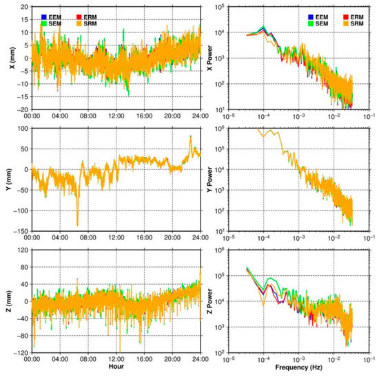
Figure 17.
Deformation monitoring time series of SHM2.
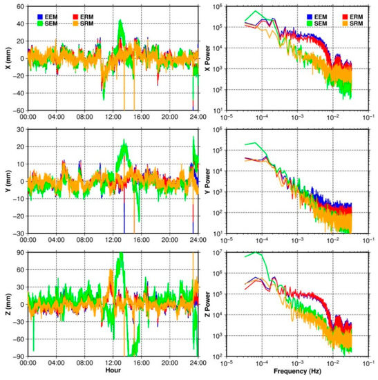
Figure 18.
Deformation monitoring time series of SHM4.
From Figure 17 except for the SEM model, the other three models generate almost the same time series and the FFT spectral results are overlapped together. Again, possibly due to the inappropriate parameters of model the SEM counterpart shows a high noise level. For SHM4, it is clearly noticed that the EEM, ERM and SRM produce the same time series, and SEM has a severe turbulence. From the FFT spectral results, the elevation related (EEM and ERM) and SNR-based (SEM and SRM) models show a quite different feature. The noise level of the results from EEM and ERM models are much higher than SEM and SRM models at the high frequency band (higher than 0.005 Hz). The severe turbulence in the result of SEM model results in a high-level noise in the low frequency band (lower than 0.0001 Hz). SRM model always shows the best results. That means, the refined SNR-based model can reasonably weight GNSS observations under obstruction conditions, which would be a great benefit for the mode parameters estimation.
5. Discussion
The refined SNR stochastic model proposed in this paper is based only on GPS and GLONASS. However, the modelling method is applicable of any other GNSS satellite systems. More studies need to be carried out to see the features of SNR data for other GNSS systems. In addition, the model proposed is also compared with the existing models in Table 1 with the high-rate observations (e.g., 10 Hz). However, no obvious difference can be seen from the high-rate displacement time series and the FFT results. Possibly, the reason is that only a few satellites are affected by the obstructions within a short period and the multipath effects could be distributed in the adjustment. Thus, the weighting performance is only shown in the low-level sampling rate data. More experiments and analysis are needed in the future to cope with the high-rate observation weighting. However, the model proposed would be more applicable to the long-term monitoring data analysis and can be used in the aspect of real-time multipath eliminating, which will also be tested and demonstrated in the future.
6. Conclusions
In this study, a refined SNR based stochastic model is proposed to weight the GNSS observations taking according of site-specific effects. The elevation dependent feature of GPS and GLONASS SNR measurements is firstly studied, and the links of SNR measurements and phase precision are analyzed. Some useful conclusions are listed as follows:
- Obvious different patterns can be observed in the GLONASS elevation-dependent SNR time series of Leica receivers. However, the phase precision has no different pattern features. That means the values of GLONASS SNR data cannot be applied to weight the phase observation directly.
- A normalized method is proposed to process the GNSS SNR data and a linear relationship between the normalized SNR data and the precision of phase observations in dual-frequency observations of GPS and GLONASS system can be observed for LEICA receivers. Hence, a linear SNR based stochastic model can be established, which is appropriate to show a precision sky-plot for assessing the site observation environment.
- Compared with the empirical elevation and SNR dependent stochastic models, and even the realistic elevation model, the refined SNR based stochastic model proposed in this paper shows the highest integer ambiguity resolution success rate in the data processing. The noise level in the data processing time series caused by obstructions can be significantly reduced with the proposed stochastic model.
Author Contributions
R.X. proposed the idea, processed the data, wrote this paper and analyzed the results of the experiments; X.M. led the GeoSHM system development; X.M. and W.J. revised the manuscript; X.A., Q.H. and Q.C. carried out the experiment and programming. All authors have read and agreed to the published version of the manuscript.
Funding
This work was supported by the National key R&D Program of China (Grant No. 2018YFC1503601) and the CRSRI Open Research Program (Program SN:CKWV2019749/KY). This research was also supported by the National Natural Science Foundation of China (Grant Nos. 41525014), and the National Science Innovation Group Foundation of China (Grant No. 41721003).
Acknowledgments
Thank goes to The Office of China Postdoctoral Council for providing the first author a scholarship under the International Postdoctoral Exchange Fellowship Program 2019 (No: 20190050) which allows him to visit the University of Nottingham for two years to research and study in the UK from October 2019. ESA is acknowledged for sponsoring GeoSHM feasibility a Demo project. Ubipos UK Ltd. is the leading company for GeoSHM Demo Project.
Conflicts of Interest
The authors declare no conflict of interest.
References
- Deng, C.; Tang, W.; Liu, J.; Shi, C. Reliable Single-Epoch Ambiguity Resolution for Short Baselines Using Combined GPS/BeiDou System. GPS Solut. 2014, 18, 375–386. [Google Scholar] [CrossRef]
- Meng, X.; Nguyen, D.; Xie, Y.; Owen, J.; Psimoulis, P.; Ince, S.; Chen, Q.; Ye, J.; Bhatia, P. Design and Implementation of a New System for Large Bridge Monitoring—GeoSHM. Sensors 2018, 18, 775. [Google Scholar] [CrossRef] [PubMed]
- Jiang, W.; Xi, R.; Chen, H.; Xiao, Y. Accuracy Analysis of Continuous Deformation Monitoring Using BeiDou Navigation Satellite System at Middle and High Latitudes in China. Adv. Space Res. 2017, 59, 843–857. [Google Scholar] [CrossRef]
- Xi, R.; Chen, H.; Meng, X.; Jiang, W.; Chen, Q. Reliable Dynamic Monitoring of Bridges with Integrated GPS and BeiDou. J. Surv. Eng. 2018, 144, 04018008. [Google Scholar] [CrossRef]
- Meng, X.; Roberts, G.W.; Dodson, A.H.; Cosser, E.; Barnes, J.; Rizos, C. Impact of GPS Satellite and Pseudolite Geometry on Structural Deformation Monitoring: Analytical and Empirical Studies. J. Geod. 2004, 77, 809–822. [Google Scholar] [CrossRef]
- Moschas, F.; Stiros, S. Dynamic Multipath in Structural Bridge Monitoring: An Experimental Approach. GPS Solut. 2014, 18, 209–218. [Google Scholar] [CrossRef]
- Zimmermann, F.; Eling, C.; Kuhlmann, H. Empirical Assessment of Obstruction Adaptive Elevation Masks to Mitigate Site-Dependent Effects. GPS Solut. 2017, 21, 1695–1706. [Google Scholar] [CrossRef]
- Dong, D.; Wang, M.; Chen, W.; Zeng, Z.; Song, L.; Zhang, Q.; Cai, M.; Cheng, Y.; Lv, J. Mitigation of Multipath Effect in GNSS Short Baseline Positioning by the Multipath Hemispherical Map. J. Geod. 2016, 90, 255–262. [Google Scholar] [CrossRef]
- Amiri-Simkooei, A.R.; Jazaeri, S.; Zangeneh-Nejad, F.; Asgari, J. Role of Stochastic Model on GPS Integer Ambiguity Resolution Success Rate. GPS Solut. 2016, 20, 51–61. [Google Scholar] [CrossRef]
- Li, B. Stochastic Modeling of Triple-Frequency BeiDou Signals: Estimation, Assessment and Impact Analysis. J. Geod. 2016, 90, 593–610. [Google Scholar] [CrossRef]
- Li, B.; Zhang, L.; Verhagen, S. Impacts of BeiDou Stochastic Model on Reliability: Overall Test, w-Test and Minimal Detectable Bias. GPS Solut. 2017, 21, 1095–1112. [Google Scholar] [CrossRef]
- Luo, X.; Mayer, M.; Heck, B. Improving the Stochastic Model of GNSS Observations by Means of SNR-Based Weighting. In Observing our Changing Earth; Sideris, M.G., Ed.; Springer: Berlin/Heidelberg, Germany, 2009; pp. 725–734. [Google Scholar]
- Agnew, D.C.; Larson, K.M. Finding the Repeat Times of the GPS Constellation. GPS Solut. 2006, 11, 71–76. [Google Scholar] [CrossRef]
- Atkins, C.; Ziebart, M. Effectiveness of Observation-Domain Sidereal Filtering for GPS Precise Point Positioning. GPS Solut. 2016, 20, 111–122. [Google Scholar] [CrossRef]
- Choi, K.; Bilich, A.; Larson, K.M.; Axelrad, P. Modified Sidereal Filtering: Implications for High-Rate GPS Positioning: HIGH-RATE GPS POSITIONING. Geophys. Res. Lett. 2004, 31. [Google Scholar] [CrossRef]
- Larson, K.M.; Bilich, A.; Axelrad, P. Improving the Precision of High-Rate GPS. J. Geophys. Res. 2007, 112, B05422. [Google Scholar] [CrossRef]
- Ragheb, A.E.; Clarke, P.J.; Edwards, S.J. GPS Sidereal Filtering: Coordinate- and Carrier-Phase-Level Strategies. J. Geod. 2007, 81, 325–335. [Google Scholar] [CrossRef]
- Wang, D.; Meng, X.; Gao, C.; Pan, S.; Chen, Q. Multipath Extraction and Mitigation for Bridge Deformation Monitoring Using a Single-Difference Model. Adv. Space Res. 2017, 60, 2882–2895. [Google Scholar] [CrossRef]
- Zhong, P.; Ding, X.; Yuan, L.; Xu, Y.; Kwok, K.; Chen, Y. Sidereal Filtering Based on Single Differences for Mitigating GPS Multipath Effects on Short Baselines. J. Geod. 2010, 84, 145–158. [Google Scholar] [CrossRef]
- Pugliano, G.; Robustelli, U.; Rossi, F.; Santamaria, R. A New Method for Specular and Diffuse Pseudorange Multipath Error Extraction Using Wavelet Analysis. GPS Solut. 2016, 20, 499–508. [Google Scholar] [CrossRef]
- Satirapod, C.; Rizos, C. Multipath Mitigation by Wavelet Analysis For GPS Base Station Applications. Surv. Rev. 2005, 38, 2–10. [Google Scholar] [CrossRef]
- Zhong, P.; Ding, X.L.; Zheng, D.W.; Chen, W.; Huang, D.F. Adaptive Wavelet Transform Based on Cross-Validation Method and Its Application to GPS Multipath Mitigation. GPS Solut. 2008, 12, 109–117. [Google Scholar] [CrossRef]
- Ge, L.; Chen, H.-Y.; Han, S.; Rizos, C. Adaptive Filtering of Continuous GPS Results. J. Geod. 2000, 74, 572–580. [Google Scholar] [CrossRef]
- Zheng, D.W.; Zhong, P.; Ding, X.L.; Chen, W. Filtering GPS Time-Series Using a Vondrak Filter and Cross-Validation. J. Geod. 2005, 79, 363–369. [Google Scholar] [CrossRef]
- Fuhrmann, T.; Luo, X.; Knöpfler, A.; Mayer, M. Generating Statistically Robust Multipath Stacking Maps Using Congruent Cells. GPS Solut. 2015, 19, 83–92. [Google Scholar] [CrossRef]
- Moore, M.; Watson, C.; King, M.; McClusky, S.; Tregoning, P. Empirical Modelling of Site-Specific Errors in Continuous GPS Data. J. Geod. 2014, 88, 887–900. [Google Scholar] [CrossRef]
- Brunner, F.K.; Hartinger, H.; Troyer, L. GPS Signal Diffraction Modelling: The Stochastic SIGMA-δ Model. J. Geod. 1999, 73, 259–267. [Google Scholar] [CrossRef]
- Bilich, A.; Larson, K.M.; Axelrad, P. Modeling GPS Phase Multipath with SNR: Case Study from the Salar de Uyuni, Boliva. J. Geophys. Res. 2008, 113, B04401. [Google Scholar] [CrossRef]
- Benton, C.J.; Mitchell, C.N. Isolating the Multipath Component in GNSS Signal-to-Noise Data and Locating Reflecting Objects: ISOLATE GNSS MULTIPATH, LOCATE REFLECTOR. Radio Sci. 2011, 46. [Google Scholar] [CrossRef]
- Groves, P.D.; Jiang, Z. Height Aiding, C/N 0 Weighting and Consistency Checking for GNSS NLOS and Multipath Mitigation in Urban Areas. J. Navig. 2013, 66, 653–669. [Google Scholar] [CrossRef]
- Peyraud, S.; Bétaille, D.; Renault, S.; Ortiz, M.; Mougel, F.; Meizel, D.; Peyret, F. About Non-Line-of-Sight Satellite Detection and Exclusion in a 3D Map-Aided Localization Algorithm. Sensors 2013, 13, 829–847. [Google Scholar] [CrossRef]
- Lau, L.; Cross, P. Development and Testing of a New Ray-Tracing Approach to GNSS Carrier-Phase Multipath Modelling. J. Geod. 2007, 81, 713–732. [Google Scholar] [CrossRef]
- Groves, P.D.; Jiang, Z.; Wang, L.; Ziebart, M.K. Intelligent Urban Positioning Using Multi-Constellation GNSS with 3D Mapping and NLOS Signal Detection. In Proceedings of the 25th International Technical Meeting of the Satellite Division of The Institute of Navigation (ION GNSS 2012), Nashville, TN, USA, 17–21 September 2012; pp. 458–472. [Google Scholar]
- Groves, P.D.; Jiang, Z.; Rudi, M.; Strode, P. A Portfolio Approach to NLOS and Multipath Mitigation in Dense Urban Areas. In Proceedings of the 26th International Technical Meeting of the Satellite Division of The Institute of Navigation (ION GNSS+ 2013), Nashville Convention Center, Nashville, TN, USA, 16–20 September 2013; pp. 3231–3247. [Google Scholar]
- Hsu, L.-T.; Jan, S.-S.; Groves, P.D.; Kubo, N. Multipath Mitigation and NLOS Detection Using Vector Tracking in Urban Environments. GPS Solut. 2015, 19, 249–262. [Google Scholar] [CrossRef]
- Strode, P.R.R.; Groves, P.D. GNSS Multipath Detection Using Three-Frequency Signal-to-Noise Measurements. GPS Solut. 2016, 20, 399–412. [Google Scholar] [CrossRef]
- Hartinger, H.; Brunner, F.K. Variances of GPS Phase Observations: The SIGMA-ɛ Model. GPS Solut. 1999, 2, 35–43. [Google Scholar] [CrossRef]
- Xi, R.; Meng, X.; Jiang, W.; An, X.; Chen, Q. GPS/GLONASS Carrier Phase Elevation-Dependent Stochastic Modelling Estimation and Its Application in Bridge Monitoring. Adv. Space Res. 2018, 62, 2566–2585. [Google Scholar] [CrossRef]
- Herring, T.A.; King, R.W.; McClusky, S.C. Gamit Reference Manual: GPS Analysis at MIT, Release 10.4; CAMBRIDGE M A.Department of Earth, Atmospheric, and Planetary Sciences, Massachusset Institute of Technology: Cambridge, MA, USA, 2010. [Google Scholar]
- Pan, L.; Xiaohong, Z.; Fei, G. Ambiguity Resolved Precise Point Positioning with GPS and BeiDou. J. Geod. 2017, 91, 25–40. [Google Scholar] [CrossRef]
- Qian, K.; Wang, J.; Hu, B. A Posteriori Estimation of Stochastic Model for Multi-Sensor Integrated Inertial Kinematic Positioning and Navigation on Basis of Variance Component Estimation. J. Glob. Position. Syst. 2016, 14, 5. [Google Scholar] [CrossRef]
- Dai, W.; Ding, X.; Zhu, J. Comparing GPS Stochastic Models Based on Observation Quality Indices. Geomat. Inf. Sci. Wuhan Univ. 2008, 33, 718–722. [Google Scholar]


© 2020 by the authors. Licensee MDPI, Basel, Switzerland. This article is an open access article distributed under the terms and conditions of the Creative Commons Attribution (CC BY) license (http://creativecommons.org/licenses/by/4.0/).