Article

Performance Evaluation of Troposphere Estimated from Galileo-Only Multi-Frequency Observations

1
Geodetic Observatory Pecný, RIGTC, Ústecká 98, 250 66 Zdiby, Czech Republic
2
School of Remote Sensing and Geomatics Engineering, Nanjing University of Information Science and Technology, Nanjing 210044, China
*
Author to whom correspondence should be addressed.
Remote Sens. 2020, 12(3), 373; https://doi.org/10.3390/rs12030373
Submission received: 29 November 2019 / Revised: 14 January 2020 / Accepted: 21 January 2020 / Published: 23 January 2020
(This article belongs to the Special Issue Global Navigation Satellite Systems for Earth Observing System)

Abstract

:
The tropospheric delays estimated from the Global Navigation Satellite System (GNSS) have been proven to be an efficient product for monitoring variations of water vapor, which plays an important role in meteorology applications. The operational GNSS water vapor monitoring system is currently based on the Global Positioning System (GPS) and GLObal NAvigation Satellite System(GLONASS) dual-frequency observations. The Galileo satellite navigation system has been evolving continuously, and on 11 February 2019, the constellation reached 22 active satellites, achieving a capability of standalone Precise Point Positioning (PPP) and tropospheric estimation that is global in scope. This enhancement shows a 37% improvement if the precision of the Galileo-only zenith tropospheric delay, while we may anticipate further benefits in terms of tropospheric gradients and slant delays in the future if an optimal multi-constellation and multi-frequency processing strategy is used. First, we analyze the performance of the multi-frequency troposphere estimates based on the PPP raw observation model by comparing it with the standard ionosphere-free model. The performance of the Galileo-only tropospheric solution is then validated with respect to GPS-only solution using 48 globally distributed Multi-GNSS Experiment (MGEX) stations. The averaged bias and standard deviations are −0.3 and 5.8 mm when only using GPS satellites, respectively, and 0.0 and 6.2 mm for Galileo, respectively, when compared to the International GNSS Service (IGS) final Zenith Troposphere Delay(ZTD) products. Using receiver antenna phase center corrections from the corresponding GPS dual-frequency observations does not affect the Galileo PPP ambiguity float troposphere solutions. These results demonstrate a comparable precision achieved for both Galileo-only and GPS-only ZTD solutions, however, horizontal tropospheric gradients, estimated from standalone GPS and Galileo solutions, still show larger discrepancies, mainly due to their being less Galileo satellites than GPS satellites. Including Galileo E1, E5a, E5b, and E5 signals, along with their proper observation weighting, show the benefit of multi-frequency observations, further improving the ZTD precision by 4% when compared to the dual-frequency raw observation model. Overall, the presented results demonstrate good prospects for the application of multi-frequency Galileo observations for the tropospheric parameter estimates.

Graphical Abstract

1. Introduction

Tropospheric delay refers to the refraction of the microwave signal when it passes through the neutral atmosphere. The space-borne microwave techniques, including Global Navigation Satellite Systems (GNSS), Very Long Baseline Interferometry (VLBI), Doppler Orbitography, and Radiopositioning Integrated by Satellite (DORIS), or Synthetic Aperture Radar Interferometry (InSAR), are all subjected to tropospheric delays [1]. GNSS has been proven to be an efficient tool for the retrieval of total tropospheric delays between the observing station and the satellites in view. The observed slant path delays are usually mapped into the zenith direction (zenith total delay, ZTD) at a GNSS station, and it comprises contributions from a hydrostatic and a wet (or more precisely non-hydrostatic) component. The ZTD typically ranges between 2.0 to 2.6 m, and 90% of the ZTD error is caused by the zenith hydrostatic delay (ZHD), which can be corrected with an a priori value from a standard atmosphere model. The zenith-wet delay (ZWD) is then usually estimated from observations as an unknown parameter with an appropriate stochastic model.
The application of high-resolution tropospheric models in Precise Point Positioning (PPP) enhances the coordinates’ accuracy and makes the convergence time of the position solution shorter (Hadas et al. [2]). Shi et al. [3] modelled the local troposphere with a set of fitting coefficients and then used it to enhance the PPP. The results indicated that the convergence time of the positioning solutions could be greatly reduced, in particular in the height component. Furthermore, de Oliveira et al. [4] confirmed the benefits of the troposphere augmentation for PPP convergence and precision improvement. Zhou et al. [5] demonstrated a better positioning accuracy of multi-GNSS PPP when estimating high-resolution tropospheric gradients. Han et al. [6] presented the accuracy improvement in the height component when using the external tropospheric delay to enhance the ambiguity-fixed PPP. Besides, investigations have been focused on the combination of a numerical weather model (NWM) and GNSS tropospheric products to enhance PPP. Lu et al. [7] developed an NWM-constrained PPP processing system to improve multi-GNSS precise positioning and demonstrated the contribution of the NWM model. Lu et al. [8] also derived horizontal delay gradients from the NWM model to augment the BeiDou System (BDS) PPP, and more than 30% of the precision improvement in the height component was observed. Zheng et al. [9] developed a real-time tropospheric model in China and used it to shorten the convergence of BDS PPP. Douša et al. [10] developed a two-stage correction tropospheric model combining data from NWM, precise GNSS ZTDs, and horizontal gradients to support an optimal regional augmentation.
High-precision troposphere observables are prerequisites for any local tropospheric model. Multi-GNSS observations have been intensively used to improve the precision of the tropospheric parameters retrieved from the PPP technique. Lu et al. [11] evaluated the performance of the real-time ZTD estimated from single and multi-GNSS observations, and the results indicated that the precision and reliability of the troposphere estimates could be improved by using multi-GNSS data. Lu et al. [12] further demonstrated that the initialization time and the precision of multi-GNSS tropospheric delays could be improved by using the PPP ambiguity-fixing technique, which can meet the requirements of the troposphere estimates for time-critical meteorological applications. Pan and Guo [13] compared the real-time troposphere solution based on different GNSS combinations and different processing models.
However, operational troposphere solutions are still mainly based on Global Positioning System (GPS) and GLObal NAvigation Satellite System (GLONASS) ionosphere-free linear combinations of dual-frequency observations. The main reason is that the performance of the new GNSS constellations, including BDS and Galileo, for troposphere estimation deserve assessment and improvement. Xu et al. [14] assessed the ZTD performance estimated from the BDS-2 regional constellation. Li et al. [15] assessed the precision of precipitable water vapor calculated from BDS-only observations and demonstrated the potential of BDS observations for high precision meteorological applications in Asia–Pacific regions. Due to the limited number of Galileo satellites, the performance of Galileo-only troposphere solution has not yet been evaluated. Until 14/12/2019, the Galileo constellation has reached 24 satellites, which enables the Galileo-only global positioning. Hadas et al. [16] have compared the positioning accuracy using dual-frequency Galileo observations and different processing techniques. An important innovation of the Galileo system is the availability of signals using five frequencies centered at E1 (1575.42 MHz), E5a (1176.45 MHz), E5b (1207.14 MHz), E5 (1191.795 MHz), and E6 (1278.75 MHz) for commercial and civilian use [17], and they are already available from all active satellites. Moreover, the introduction of an Alternate Binary Offset Carrier (AltBOC) signal is expected to deliver smaller pseudorange noise thanks to its large bandwidth. The availability of multi-frequency signals has been proven to bring a great opportunity for PPP ambiguity resolution. Liu et al. [18] demonstrated that the Galileo triple-frequency PPP, with ambiguity resolution, was helpful in reducing the convergence time and to improve the positioning accuracy. Li et al. [19] also showed that the average Time To the First Fix (TTFF) of triple-frequency PPP can be reduced by more than 10%, compared to the dual-frequency solutions. Moreover, the results indicate that the fractional parts of extra-wide-lane ambiguities for all Galileo satellites are all zero, which may be associated with the characteristic of the AltBOC signal. Li et al. [20] analyzed the multi-frequency PPP ambiguity resolution method based on the Galileo five-frequency observations. While the use of more frequencies contributes in a minor way to the TTFF, decimeter-level positioning accuracy can be achieved within 0.5 min by utilizing triple-/quad-/five-frequency PPP wide-lane ambiguity resolution. In comparison, the benefits of the multi-frequency observations for troposphere estimations still deserve further investigation.
In this contribution, we investigate the performance of the standalone Galileo troposphere estimates and the impact of multi-frequency observations. The paper is organized as follows: After this introduction, the PPP-based ionosphere-free and raw-observation troposphere estimation methods are introduced. Next, the precision of the Galileo-only ZTD and gradient solutions are compared to the GPS solution. Then, we characterize the noise of Galileo code observations residuals from multiple frequencies, and analyze the impact of multi-frequency observations on the accuracy of estimated ZTD. Finally, the conclusions are derived.

2. GNSS Troposphere Estimation Methods

First, generally used raw-observation (RAW) and ionosphere-free (IF) PPP models for the troposphere estimation are introduced. Second, we provide details of the processing strategy and the software.

2.1. Functional Model

Raw code and carrier phase observations can be expressed as follows:
P r , i s = ρ r s + d t r d t s + T r s + μ i I r , 1 s + ε i , P s L r , i s = ρ r s + d t r d t s + T r s μ i I r , 1 s + λ i N r , i s + ε i , L s
where the subscript r and s represent the receiver and satellite, respectively; i denotes the observation frequency; P r , i s and L r , i s denote the raw code and carrier phase observation in meters, respectively; ρ r s denotes the geometric distance between the receiver and the satellite; d t r denotes the receiver clock error; d t s denotes the satellite clock error; I r , 1 s denotes the slant ionospheric delay on the first frequency; μ i = f 1 2 / f i 2 denotes the frequency-related constant value; T r s denotes the slant tropospheric delay; N r , i s and λ i denotes the phase ambiguities and corresponding wavelength; and ε i , P s and ε i , L s denote the sum of multipath error and measurement noise for code and phase observables, respectively. Note that the code and phase observations are both affected by the hardware delays. The code hardware delays should be corrected using IGS differential code biases (DCB) products, whereas the phase hardware delays are absorbed by the ambiguity parameter.
The raw observation model in Equation (1) can be used flexibly for multi-frequency observations without considering the correlation between the observations. The model can retain the full advantages of multi-frequency observations, including the analyses of individual signal characteristics and observation weighting, as well as significantly lower observation noise of the original measurements, compared to any linear combination. However, the satellite-specific ionospheric delays have to be estimated as unknown parameters. In comparison, the ionosphere-free (IF) linear combination enables the elimination of the first-order ionospheric effect. The generalized dual-frequency IF model can be expressed as:
P r , c s = ρ r s + d t r d t s + T r s + ε P s L r , c s = ρ r s + d t r d t s + T r s + λ c N r , c s + ε L s
where λ c and N c represent the IF wavelength and the corresponding ambiguity, respectively. However, the modeling of triple-frequency PPP using two dependent IF linear combinations needs to account for the correlations between observations [21,22]. Moreover, the observation noise is increased for both code and phase observations.
The satellite orbit and clock offsets in Equations (1) and (2) are usually introduced from external real-time or final precise products. The other terms should be properly estimated as unknown parameters after applying all the necessary corrections, including the tidal effects, antenna satellite antenna phase center offsets (PCOs) and variations (PCVs), phase wind up, and others. The slant tropospheric delay T r s can be written as a sum of hydrostatic, wet, and gradient delays, which is expressed in Equation (3):
T r s = m H Z H D + m W Z W D + m G G N cos A + G E sin A
where A is an azimuth angle of a satellite; Zenith Hydrostatic Delay (ZHD) and Zenith Wet Delay (ZWD) are hydrostatic and wet contributions of the ZTD; m H and m W are corresponding hydrostatic and wet mapping functions; G N , G E are tropospheric gradients in the North and East directions; and m G is their mapping function. While ZHD is introduced using an empirical model, e.g., Saastamoinen [23], ZWD and horizontal gradients are estimated as unknowns, along with other parameters in the PPP processing.

2.2. Processing Strategies

We used the G-Nut/Tefnut software developed at the Geodetic Observatory Pecny (GOP) [24] for the multi-GNSS data processing. The software has met the requirements for real-time multi-GNSS troposphere estimation for meteorological applications [25]. The tropospheric parameters in a high temporal resolution, including ZTDs, horizontal tropospheric gradients, and slant path delays, can be estimated in both real-time and near real-time processing modes [26]. Two estimators are supported: A forward Kalman filter for the real-time processing and a backward smoother to improve the precision of the troposphere [27] in the case of post-processing or near real-time. The software was recently enhanced with the capability of multi-frequency processing, based on the raw observation model. The selection of frequencies, observation types, and channels are enabled with the XML configuration file. Table 1 lists the details of various processing strategies implemented in the software. The satellite and receiver antenna phase center (PCO) and antenna phase variations (PCV) are applied for GPS L1/L2, GLONASS L1/L2, and Galileo E1/E5a frequencies. If the receiver PCO and PCV are not available for a specific station, the corresponding GPS corrections are used. We only processed signals from healthy satellites for real-time troposphere estimation, whereas all satellites provided by the final products are used in the post-processed solutions.

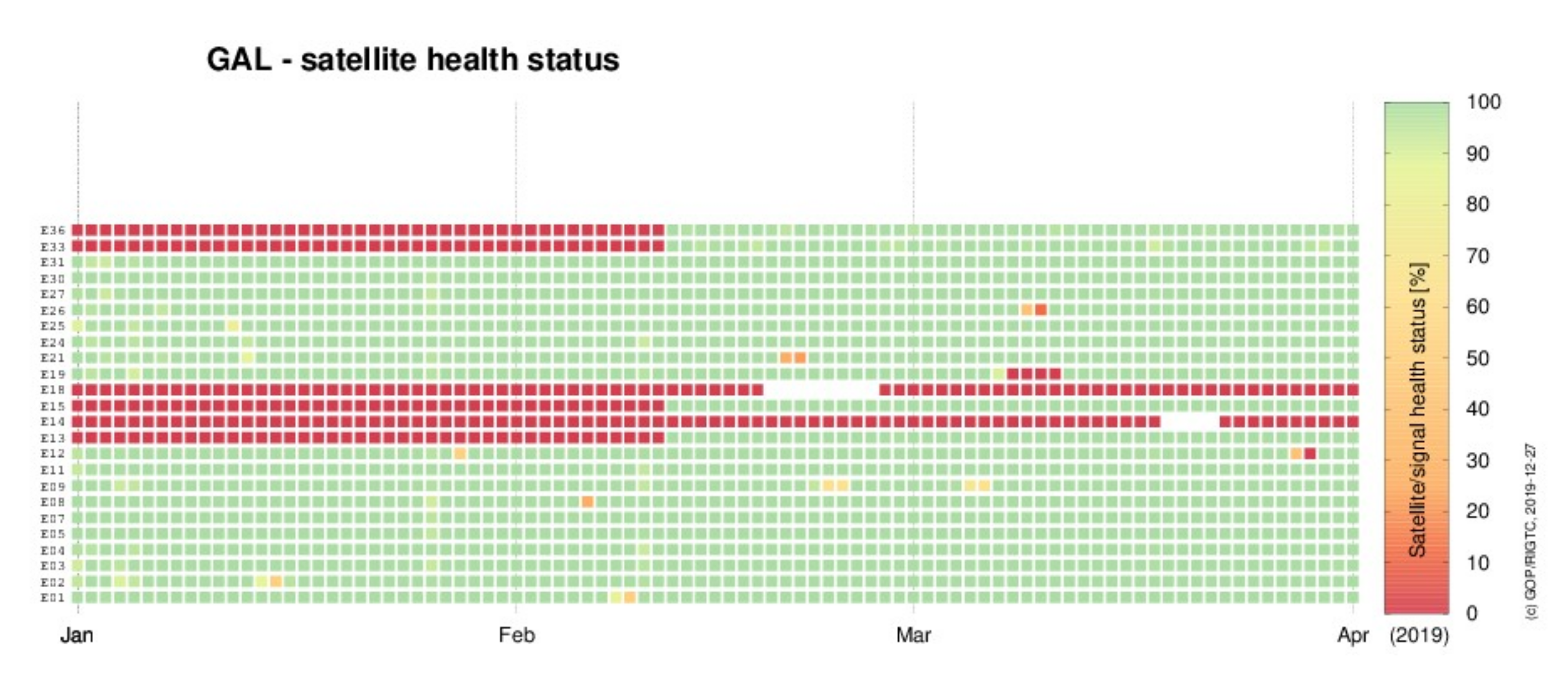
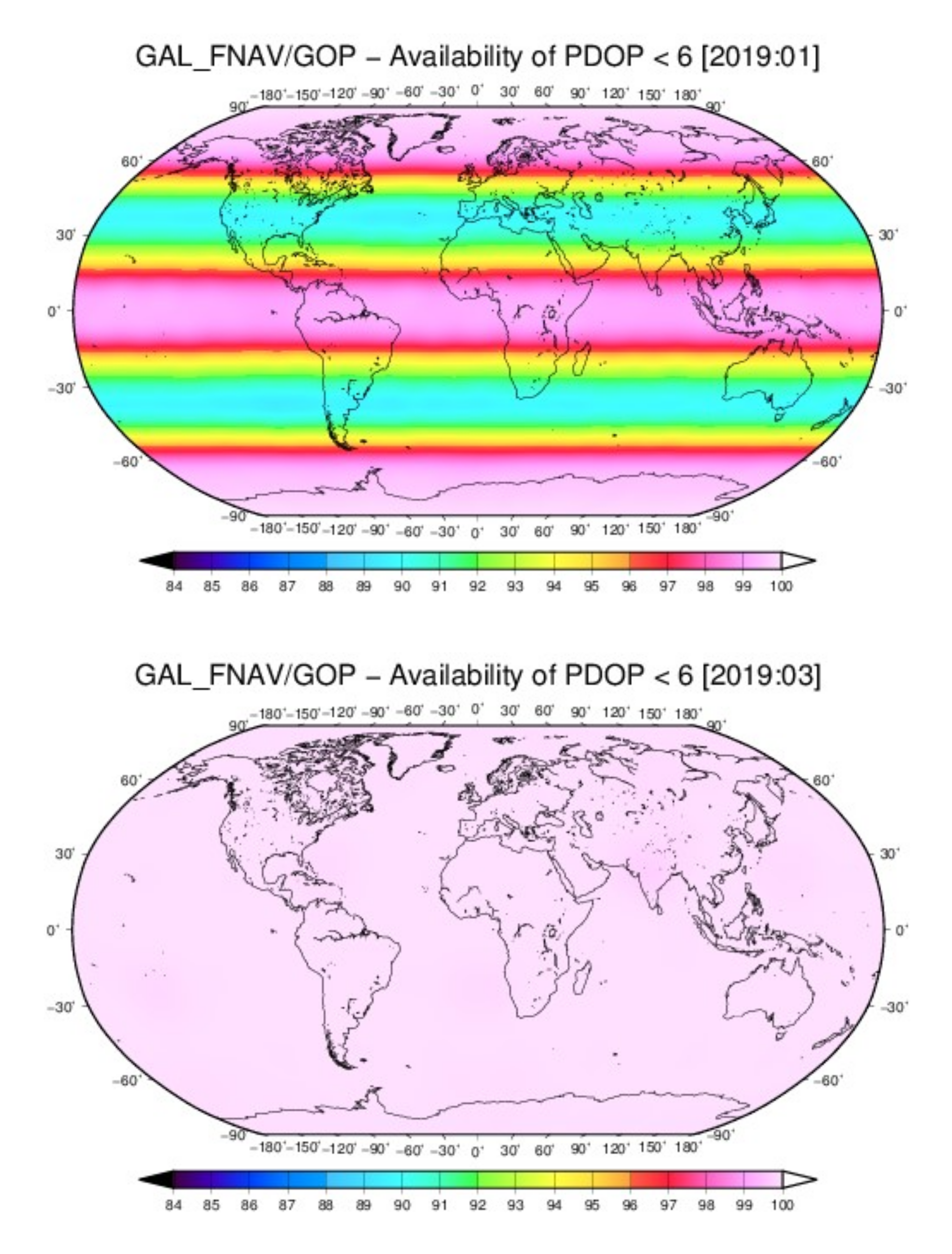
3. Status of Standalone Galileo Troposphere Solution

The Galileo system Initial Services was announced on 15 December 2016, and it is expected to be completed for full operational capability (FOC) in 2020. However, the Galileo system achieved an important milestone when the constellation reached, altogether, 26 satellites after the successful launch of Ariane-5 on 25 July 2018. Four new Galileo satellites (E13, E15, E33, and E36) became healthy on 11 February 2019, when the Galileo constellation reached 22 active satellites, two satellites on highly eccentric orbits in testing mode (E14 and E18), one satellite that was unavailable (E20), and one satellite that was excluded from the constellation (E22). The constellation change in the first quarter of 2019 is clearly depicted in Figure 1. The color represents a daily percentage of navigation messages, indicating a healthy status of the Signal-In-Space for each satellite when considering: 1) The Signal Health Status flag (SHS), 2) the Data Validity Status flag (DVS), 3) Signal-In-Space Accuracy (SISA) value, and 4) the navigation data validity period [28]. Note that the satellite health status can be used as an indicator for the quality of the satellite broadcast ephemeris, which is important for real-time users. However, MGEX final products are using the satellite signals even when they are unhealthy, since robust quality control strategies can be used to identify the actual status of the satellites by post-processing.
The Position Dilution Of Precision (PDOP) is calculated on a regular grid of 10 x 10 degrees, considering healthy Galileo satellites and the 5-degree elevation mask cut-off. Figure 2 shows the change in the monthly mean availability of PDOP < 6 for the Galileo system on a global scale between January and March. Four new satellites dramatically improved the availability of PDOP less than 6, reaching almost 100% globally in March, 2019.
The impact of such a constellation improvement on the tropospheric parameters is demonstrated via the comparison of the multi-GNSS solution with the standalone PPP solutions using only satellites from individual systems, namely GPS, GLONASS, and Galileo. We processed observations from 215 days (from October 27, 2018 to May 30, 2019) to demonstrate the evolution of the Galileo standalone troposphere solution. The final orbit and clock products provided by the Center for Orbit Determination in Europe (CODE) within Multi-GNSS Experiment (MGEX) project were used for PPP troposphere estimates when using the IF linear combinations with float ambiguities. The troposphere product exploiting combined GPS/GLONASS/Galileo observations was used as a reference. The selection of multi-GNSS combined troposphere solutions, rather than the external tropospheric products, as the reference was to demonstrate the consistency of GPS/Galileo/GLONASS standalone tropospheric with respect to the combined solutions. The standard deviation (STD) of the differences between the reference solution and Galileo-only troposphere solution presented in Figure 3 illustrates the visible change of STD for station ZIM2 and GOP6. A clear improvement can be observed after the four new Galileo satellites became available. The average STDs before February 11 was 4.3 and 5.0 mm for stations ZIM2 and GOP6, respectively. Significant decreases were observed after 11 February 2019, reaching 2.7 and 2.7 mm, respectively. Figure 4 presents the evaluation of GPS, GLONASS, and Galileo standalone ZTD solutions, as compared to the multi-GNSS solution. The dark and light colors represent the results before and after 2019–02–11, respectively. Overall, GPS-only ZTD had the best precision compared to the GLONASS-only and Galileo-only solution in the two stations before 2019–02–11. After that, the Galileo-only ZTD solution achieved comparable precision, like the GPS-only solution for the two stations. However, the GLONASS ZTD solution was always worse than that of GPS and Galileo. Precision improvement can be observed for three different ZTD solutions after 2019–02–11, which can attribute to the improvement of the reference multi-GNSS ZTD solutions after the availability of new Galileo satellites.

4. Evaluation of Troposphere Estimated from Multi-Frequency Galileo Observations

The dual-frequency IF combinations are commonly used for the PPP troposphere estimates. With the availability of observations from multiple frequencies, some groups have focused on combining two L1/L2 and L1/L5 IF combinations in the case of GPS satellites. However, the correlation between the observations has to be considered. Besides, the triple-frequency IF combination [29] cannot be flexibly extended for the processing of more frequencies. The raw-observation PPP model has two main benefits: 2) Lower observation noise and 2) full flexibility in terms of the multi-frequency processing. To assess the benefits of using the raw PPP model and multi-frequency observations for tropospheric parameter estimation, two questions are first clarified: (1) Can the troposphere delays estimated from both RAW and IF PPP models achieve comparable precision? (2) Can the Galileo-only tropospheric delays achieve comparable precision compared to the GPS only solutions on a global scale? After demonstrating the achievable performance of the raw PPP model and Galileo-only tropospheric solutions, the multi-frequency Galileo ZTD solutions derived from the RAW PPP model are analyzed.

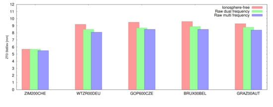
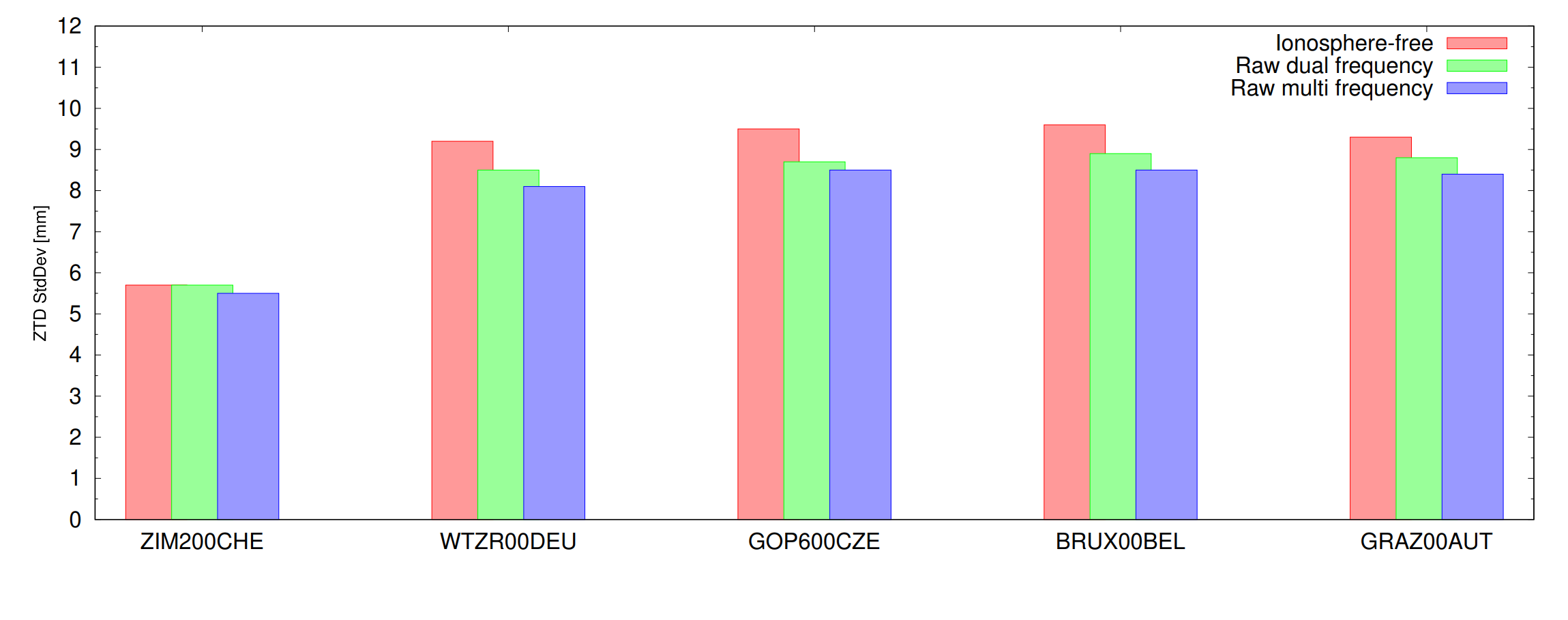
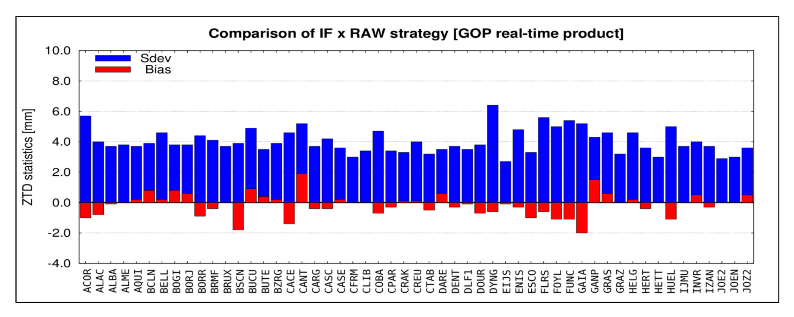
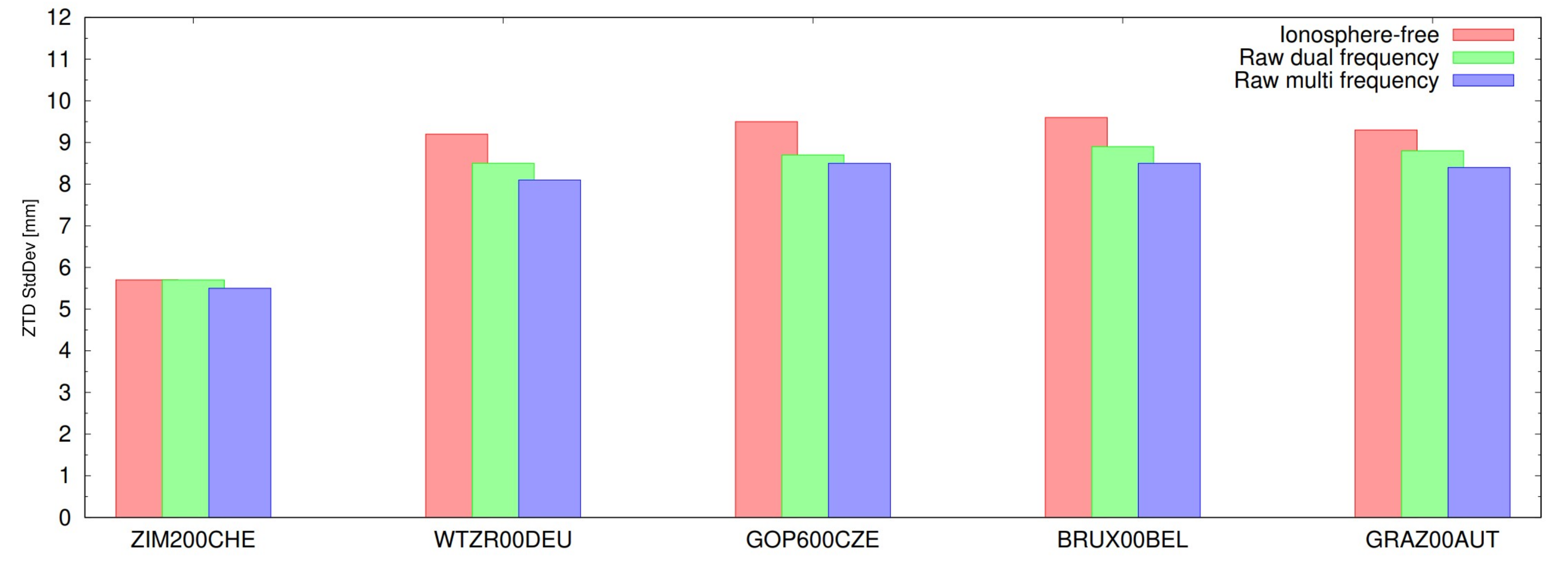
4.1. Comparison of ZTD from the IF and the RAW Model

To evaluate the accuracy of the tropospheric delay from the IF and the RAW PPP models, the results from routinely running real-time demonstration are used. The campaign was set to evaluate the performance of raw PPP for real-time troposphere estimation and meteorology applications. Figure 5 illustrates the distribution of the EPN (European Permanent Network) stations. Real-time orbit and clock products from CNES [30] and the real-time EPN observations streams are processed with the Kalman filter.
Figure 6 presents ZTD differences between the models for several selected stations. It can be observed that the tropospheric parameters are well distributed around a mean value. However, the real-time solutions are affected by a low availability of observations and corrections streams, which can be clearly observed with the gap near May 1, 2019. Figure 7 shows the overall statistics for standard deviations and biases calculated from the ZTD differences. Generally, the biases are below 2 mm, and the standard deviations are below 6 mm. The results indicate a good agreement between the ZTD estimates using RAW and IF models in routine real-time processing.

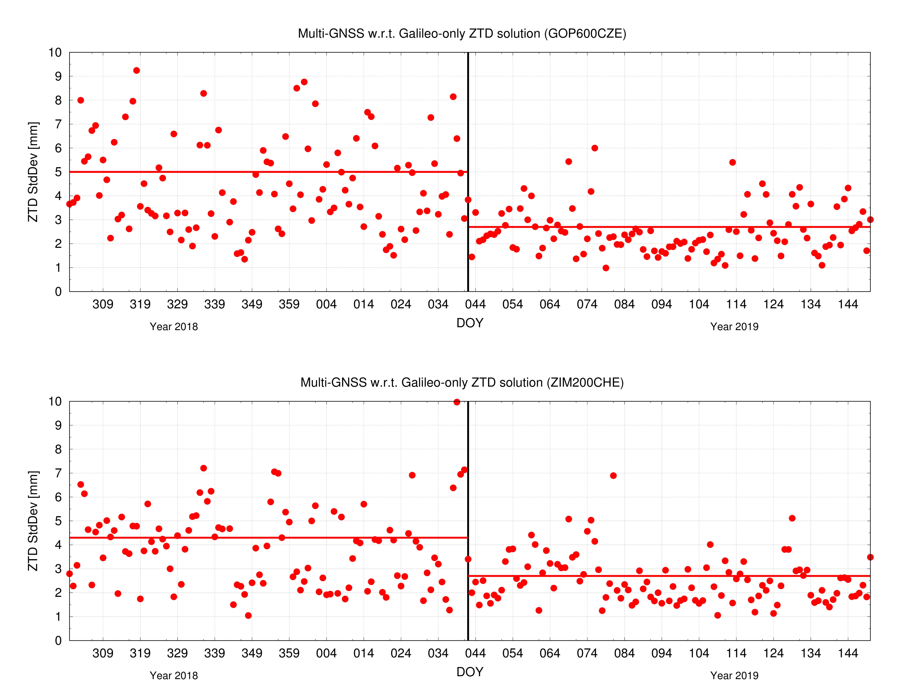
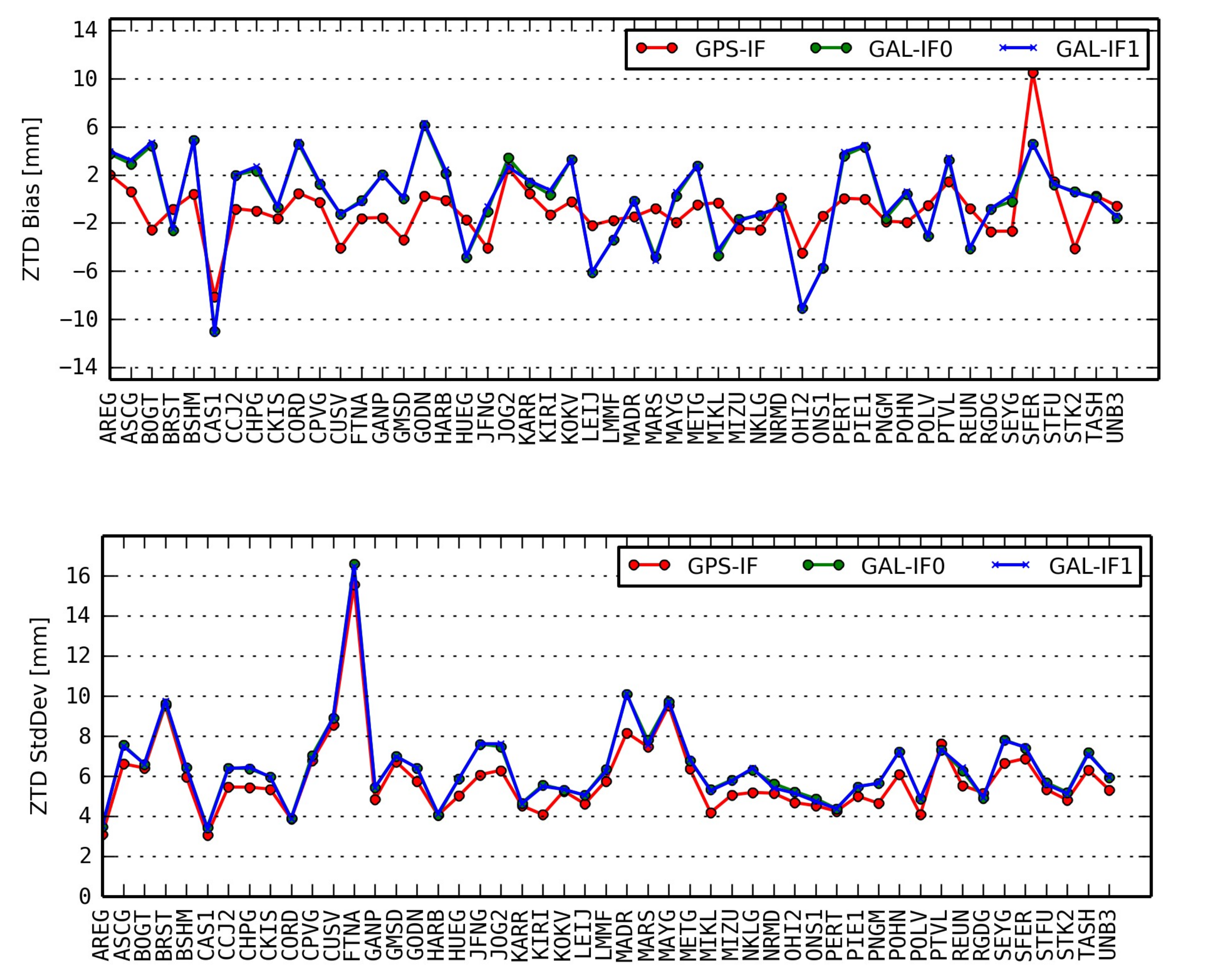
4.2. Comparison of Tropospheric Delay from the GPS-Only and Galileo-Only Solutions

To demonstrate a global performance of Galileo-only troposphere estimation, data from 48 MGEX stations were selected and processed over a two-month period (April 10–June 09, 2019). Figure 8 displays a geographical distribution of the selected global stations. Dual-frequency observations from GPS (L1, L2) and Galileo (E1, E5a) are used to create IF linear combinations within PPP troposphere estimation. Final, precise orbit and clock products from the CODE MGEX analysis center are used [31]. The station coordinates are estimated as static parameters on a daily basis. Besides, a backward filter was used to enhance the troposphere solution.
Figure 9 displays the statistics for GPS and Galileo IF ZTDs compared to the IGS tropospheric product, respectively. Mean biases for all the stations are shown at top plot, standard deviations (STD) are at the bottom plot. Strategy “GPS-IF” indicates GPS dual-frequency IF solutions. For Galileo troposphere estimation, different receiver PCO and PCV correction strategies are compared. Strategy “GAL-IF0” indicates the receiver E1 and E5a PCO, and PCV are corrected using the same values as that of GPS L1 and L2 frequencies. The strategy “GAL-IF1” corrects the receiver PCO and PCV from the IGS Reprocessing 2020 ANTEX file. Note that the Galileo receiver PCO and PCV for three stations listed in Table 2 are also not calibrated using the processing strategy “GAL-IF1”. Overall, the variations of biases and STDs from the GPS-only and Galileo-only troposphere solutions show similar patterns. It has to be emphasized here that the IGS product is based on GPS data only. The averaged mean bias over all stations is -0.3, 0.0, and 0.0 mm for “GPS-IF”, “GAL-IF0”, and “GAL-IF1”, respectively. The biases are distributed around a zero mean, varying slightly more for Galileo than GPS. For the latter, the biases were within ±4 mm, except for three stations (CAS1, SFER, and FTNA). A single value exceeding 10 mm was observed at the CAS1 station. The average STD is 5.8, 6.2, and 6.2 mm for “GPS-IF”, “GAL-IF0”, and “GAL-IF1”, respectively. A slightly worse precision in the Galileo ZTD solution can be mainly attributed to two aspects. First, the Galileo constellation counts only 22 active satellites, compared to 31 active satellites for GPS. Second, the orbit and clock products and correction models are still more accurate for GPS, compared to Galileo [32,33]. However, the Galileo-only ZTD can achieve a comparable accuracy compared to that of GPS processing.
Interestingly, the effects of the receivers PCO and PCV calibration are not obvious in the comparison of the results from processing strategies “GAL-IF0” and “GAL-IF1”, which slightly differ with the results of Reference [34], are based on the double-difference processing that a 1.8 mm difference in the mean biases of ZWD is observed for different receiver antenna phase center correction models. This is mainly due to the ambiguities being resolved as the float in the PPP filter and thus the elevation-dependent receiver PCO variations are absorbed by the ambiguities. Note that, although the ambiguities are modeled as constant in PPP during the satellite path in a view without a cycle slip, the float ambiguities can still absorb part of the remaining unmodeled errors during the least-square adjustment or the Kalman filter procedure.
The tropospheric gradients reflect a local horizontal anisotropy, mainly due to an asymmetric distribution of water vapor. As Galileo can achieve a similar precision comparable to the GPS in terms of ZTD, we further compared horizontal gradient components independently of those estimated from GPS and Galileo observations. Figure 10 presents the time series of the ZWD (top), the North component (middle), and the East component (bottom) of the tropospheric gradients obtained from the GPS and Galileo-IF1 solutions for the AREG station. While a good consistency is observed for the ZWD, larger discrepancies can be observed for the gradient components. Regular jumps are observed for gradient components at the day boundaries, which are due to only estimating (and modelling) all the parameters on a daily basis. Such day-to-day inconsistency indicates a possible uncertainty of the estimated parameter. The gradient calculated with the Galileo observations show a larger variation, although it could still show similar trends compared to the GPS solution. First, it is attributed to the number of visible Galileo satellites and their geometry, which is critical for the gradient estimation. Second, Kacmarik et al. [35] analyzed the factors affecting the GNSS tropospheric gradient estimates, and indicated that the antenna-phase center offsets and variations, mapping functions, and orbit/clock quality all matter. It can thus be expected that the precision of the Galileo gradient solutions can be improved with the refinement of Galileo correction models, along with the completing of the Galileo constellation.

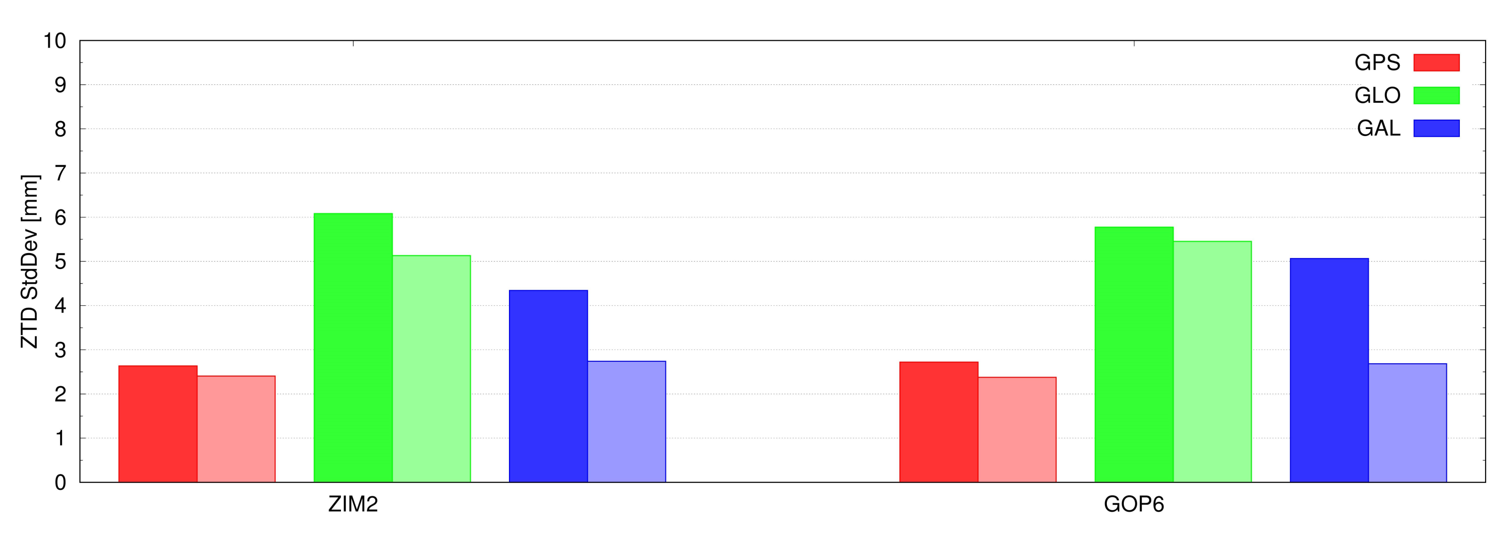
4.3. Multi-Frequency Troposphere Solutions

To demonstrate the benefits of the ZTD estimated with the RAW PPP model, three different processing strategies are defined in Table 3. The multi-frequency solution (RAW-multi) can use up to four frequency observations.
The observation post-fit residuals from the PPP processing can be used as a comprehensive indicator for the quality of GNSS precise satellite orbit/clocks, observation noise, and remaining model errors. The Galileo E5 signal indicates a significantly lower observation noise due to the AltBOC signal modulation properties. Table 4 summarizes root mean square (RMS) of estimated code signal noises from all GPS and Galileo satellites. Additionally, the noise of the IF linear combination is listed too, and as theoretically expected, is about three times larger compared to the raw observations. Anyway, the Galileo E5 observation truly indicates the best quality.
The observation weighting was then applied in assessing the impact of the multi-frequency raw-observation processing strategy on ZTD estimates. For this purpose, we used data from 5 European stations and a two-month period (April 10–June 09, 2019). The real-time orbits and clocks from CNES were used to correct the navigation satellite orbit and clock errors, and the combined troposphere solutions were used as the reference [36]. Figure 11 illustrates the standard deviations of the multi-GNSS ZTD using different strategies at selected stations. Overall, the achieved uncertainty (1-sigma) is below 9 mm for all the stations. The results using the raw dual-frequency observations slightly improved the precision of the ZTD by 6%, compared to the IF model, which can be mainly attribute to the lower noise of the raw observations. Then, by adding even more frequencies into the RAW PPP model, it is able to further improve the precision by 4%, which clearly demonstrates the benefits of multi-frequency observations such as those provided by Galileo for all the satellites. It should be emphasized that even GPS-only RAW PPP solutions should benefit from the L5 observations, even though they are still available from about a half of the satellites in 2019.

5. Conclusions

The recent evolution of the Galileo constellation has made Galileo capable of the standalone positioning and troposphere estimation. We analyzed the performance of Galileo observations for ZTDs and tropospheric horizontal gradient estimation. In addition, the benefits of multi-frequency observations are evaluated on the basis of the raw PPP model.
When four FOC satellites (E13, E15, E33, and E36) became healthy after 11 February 2019, the PDOP significantly improved, and therefore, the Galileo-only observations could be used for positioning on a global scale. The precision of the Galileo-only ZTD solution is first evaluated in comparison to the multi-GNSS solution based on two European stations. The average standard deviation of the Galileo-only ZTD solution decreased by 37% after its globally operational convergence.
As the raw model is more flexible for tropospheric parameter estimation, based on multi-frequency observations, the accuracy of raw and IF dual-frequency processing is first compared with solutions from real-time EPN RT demonstration. The results indicate that the raw dual-frequency model can achieve a comparable accuracy with the traditional IF model, with the mean biases and standard deviation of the ZTD difference below 2 and 6 mm, respectively. Additionally, the performance of the GPS-only and Galileo-only ZTD solutions are evaluated in comparison to the IGS final troposphere products, based on the globally distributed MGEX stations. The average mean biases over all stations are −0.3 and 0.0 mm for GPS and Galileo, respectively. The average STD is 5.8 and 6.2 mm for GPS and Galileo, respectively. The results demonstrate that the Galileo-only ZTD solution can achieve similar precision, compared to that of the GPS. However, the comparison of the GPS and Galileo gradient solutions indicate that Galileo still provides less accurate gradient components compared to GPS, which are expected to be improved with the refinement of the Galileo correction model. Besides, although the receiver PCO calibration is not completed for Galileo observations, using corresponding GPS PCO corrections does not degrade the PPP troposphere solutions.
After demonstrating the potential of the raw model and Galileo-only observations for ZTD estimations, the benefits of the Galileo multi-frequency observations on tropospheric parameters estimated with the raw PPP model are evaluated. The precision of the multi-frequency Galileo troposphere ZTDs is evaluated. The dual-frequency raw observations improve the precision of ZTD compared to the IF model by 6%. Besides, the addition of more frequency signals can further improve the ZTD accuracy by 4%. The results demonstrate a bright prospect for the improvement of GNSS ZTD with the additional use of Galileo multi-frequency observations.

Author Contributions

L.Z. conceived and designed the experiments and wrote most of the paper. P.V. and J.D. performed the experiments and carefully read and improved the text. All authors have read and agreed to the published version of the manuscript.

Funding

This work was supported in part by the National Project PUNTIS (Grant LO1506), and in part by the Startup Project for Introducing Talent of NUIST (under grant number:2019r081).

Acknowledgments

We acknowledge the European Union and the European GNSS Agency (GSA) for supporting the cooperation of the Galileo Reference Center (GRC) with Member States within the GRC-MS project, and co-financed as of November 2019 (Grant agreement nr. GSA/GRANT/04/2016), in support of an independent monitoring of the Galileo system performance [37, 38].

Conflicts of Interest

The authors declare no conflict of interest.

References

  1. Wilgan, K.; Geiger, A. High-resolution models of tropospheric delays and refractivity based on GNSS and numerical weather prediction data for alpine regions in Switzerland. J. Geod. 2019, 93, 819–835. [Google Scholar] [CrossRef] [Green Version]
  2. Hadas, T.; Kaplon, J.; Bosy, J.; Sierny, J.; Wilgan, K. Near-real-time regional troposphere models for the GNSS precise point positioning technique. Meas. Sci. Technol. 2013, 24, 055003. [Google Scholar] [CrossRef]
  3. Shi, J.; Xu, C.; Guo, J.; Yang, G. Local troposphere augmentation for real-time precise point positioning. Earth Planets Space 2014, 66, 1–13. [Google Scholar] [CrossRef] [Green Version]
  4. De Oliveira, P.; Morel, L.; Fund, F.; Legros, R.; Monico, J.; Durand, S.; Durand, F. Modeling tropospheric wet delays with dense and sparse network configurations for PPP-RTK. GPS Solut. 2017, 21, 237–250. [Google Scholar] [CrossRef] [Green Version]
  5. Zhou, F.; Li, X.; Li, W.; Chen, W.; Dong, D.; Wickert, J.; Schuh, H. The impact of estimating high-resolution tropospheric gradients on multi-GNSS precise positioning. Sensors 2017, 17, 756. [Google Scholar] [CrossRef] [PubMed]
  6. Han, H.; Xu, T.; Wang, J. Tightly Coupled Integration of GPS Ambiguity Fixed Precise Point Positioning and MEMS-INS through a Troposphere-Constrained Adaptive Kalman Filter. Sensors 2016, 16, 1057. [Google Scholar] [CrossRef] [Green Version]
  7. Lu, C.; Zus, F.; Ge, M.; Heinkelmann, R.; Dick, G.; Wickert, J.; Schuh, H. Tropospheric delay parameters from numerical weather models for multi-GNSS precise positioning. Atmos. Meas. Tech. 2016, 9, 5965–5973. [Google Scholar] [CrossRef] [Green Version]
  8. Lu, C.; Li, X.; Zus, F.; Heinkelmann, R.; Dick, G.; Ge, M.; Wickert, J.; Schuh, H. Improving BeiDou real-time precise point positioning with numerical weather models. J. Geod. 2017, 91, 1019–1029. [Google Scholar] [CrossRef]
  9. Zheng, F.; Lou, Y.; Gu, S.; Gong, X.; Shi, C. Modeling tropospheric wet delays with national GNSS reference network in China for BeiDou precise point positioning. J. Geod. 2018, 92, 545–560. [Google Scholar] [CrossRef]
  10. Douša, J.; Eliaš, M.; Václavovic, P.; Eben, K.; Krč, P. A two-stage tropospheric correction model combining data from GNSS and numerical weather model. Gps Solut. 2018, 22, 77. [Google Scholar] [CrossRef]
  11. Lu, C.; Chen, X.; Liu, G.; Dick, G.; Wickert, J.; Jiang, X.; Zheng, K.; Schuh, H. Real-time tropospheric delays retrieved from multi-GNSS observations and IGS real-time product streams. Remote Sens. 2017, 9, 1317. [Google Scholar] [CrossRef] [Green Version]
  12. Lu, C.; Li, X.; Cheng, J.; Dick, G.; Ge, M.; Wickert, J.; Schuh, H. Real-time tropospheric delay retrieval from multi-GNSS PPP ambiguity resolution: Validation with final troposphere products and a numerical weather model. Remote Sens. 2018, 10, 481. [Google Scholar] [CrossRef] [Green Version]
  13. Pan, L.; Guo, F. Real-time tropospheric delay retrieval with GPS, GLONASS, Galileo and BDS data. Sci. Rep. 2018, 8, 17067. [Google Scholar] [CrossRef] [PubMed] [Green Version]
  14. Xu, A.; Xu, Z.; Ge, M.; Xu, X.; Zhu, H.; Sui, X. Estimating zenith tropospheric delays from BeiDou navigation satellite system observations. Sensors 2013, 13, 4514–4526. [Google Scholar] [CrossRef] [PubMed]
  15. Li, M.; Li, W.; Shi, C.; Zhao, Q.; Su, X.; Qu, L.; Liu, Z. Assessment of precipitable water vapor derived from ground-based BeiDou observations with Precise Point Positioning approach. Adv. Space Res. 2015, 55, 150–162. [Google Scholar] [CrossRef]
  16. Hadas, T.; Kazmierski, K.; Sośnica, K. Performance of Galileo-only dual-frequency absolute positioning using the fully serviceable Galileo constellation. GPS Solut. 2019, 23, 108. [Google Scholar] [CrossRef] [Green Version]
  17. European GNSS Service Centre. Available online: http://www.gsc-europa (accessed on 23 January 2020).
  18. Liu, G.; Zhang, X.; Li, P. Improving the Performance of Galileo Uncombined Precise Point Positioning Ambiguity Resolution Using Triple-Frequency Observations. Remote Sens. 2019, 11, 341. [Google Scholar] [CrossRef] [Green Version]
  19. Li, X.; Li, X.; Liu, G.; Feng, G.; Yuan, Y.; Zhang, K.; Ren, X. Triple-frequency PPP ambiguity resolution with multi-constellation GNSS: BDS and Galileo. J. Geod. 2019, 1–18. [Google Scholar] [CrossRef]
  20. Li, X.; Liu, G.; Li, X.; Zhou, F.; Feng, G.; Yuan, Y.; Zhang, K. Galileo PPP rapid ambiguity resolution with five-frequency observations. GPS Solut. 2020, 24, 24. [Google Scholar] [CrossRef]
  21. Deo, M.; El-Mowafy, A. Triple-frequency GNSS models for PPP with float ambiguity estimation: Performance comparison using GPS. Surv. Rev. 2018, 50, 249–261. [Google Scholar] [CrossRef] [Green Version]
  22. Guo, F.; Zhang, X.; Wang, J.; Ren, X. Modeling and assessment of triple-frequency BDS precise point positioning. J. Geod. 2016, 90, 1223–1235. [Google Scholar] [CrossRef]
  23. Saastamoinen, J. Contributions to the theory of atmospheric refraction. Bull. Géod. 1973, 107, 13–34. [Google Scholar] [CrossRef]
  24. Vaclavovic, P.; Dousa, J.; Gyori, G. G-Nut software library-state of development and first results. Acta Geodyn. Geomater. 2013, 10, 431–436. [Google Scholar] [CrossRef] [Green Version]
  25. Dousa, J.; Vaclavovic, P. Real-time zenith tropospheric delays in support of numerical weather prediction applications. Adv. Space Res. 2014, 53, 1347–1358. [Google Scholar] [CrossRef]
  26. Douša, J.; Václavovic, P.; Zhao, L.; Kačmařík, M. New adaptable all-in-one strategy for estimating advanced tropospheric parameters and using real-time orbits and clocks. Remote Sens. 2018, 10, 232. [Google Scholar] [CrossRef] [Green Version]
  27. Vaclavovic, P.; Dousa, J. Backward smoothing for precise GNSS applications. Adv. Space Res. 2015, 56, 1627–1634. [Google Scholar] [CrossRef]
  28. European GNSS (Galileo) Initial Service, Open Service (OS) Service Definition Document (SDD), Issue 1.1, European Union, May 2019. Available online: http://www.gsc-europa.eu (accessed on 23 January 2020).
  29. Han, S.; Rizos, C. The Impact of Two Additional Civilian GPS Frequencies on Ambiguity Resolution Strategies. In 55th National Meeting US Institute of Navigation, “ Navigational Technology for the 21st Century”; The Institute of Navigation: Manassas, VA, USA, 2000; pp. 28–30. [Google Scholar]
  30. Loyer, S.; Perosanz, F.; Mercier, F.; Capdeville, H.; Marty, J.-C. Zero-difference GPS ambiguity resolution at CNES–CLS IGS Analysis Center. J. Geod. 2012, 86, 991–1003. [Google Scholar] [CrossRef]
  31. Prange, L.; Dach, R.; Lutz, S.; Schaer, S.; Jäggi, A. The CODE MGEX Orbit and Clock Solution; Springer: Cham, Switzerland, 2015; pp. 767–773. [Google Scholar] [CrossRef] [Green Version]
  32. Kazmierski, K.; Sośnica, K.; Hadas, T. Quality assessment of multi-GNSS orbits and clocks for real-time precise point positioning. GPS Solut. 2018, 22, 11. [Google Scholar] [CrossRef] [Green Version]
  33. Guo, F.; Li, X.; Zhang, X.; Wang, J. Assessment of precise orbit and clock products for Galileo, BeiDou, and QZSS from IGS Multi-GNSS Experiment (MGEX). GPS Solut. 2017, 21, 279–290. [Google Scholar] [CrossRef]
  34. Ejigu, Y.G.; Hunegnaw, A.; Abraha, K.E.; Teferle, F.N. Impact of GPS antenna phase center models on zenith wet delay and tropospheric gradients. GPS Solut. 2019, 23. [Google Scholar] [CrossRef]
  35. Kacmarik, M.; Dousa, J.; Zus, F.; Vaclavovic, P.; Balidakis, K.; Dick, G.; Wickert, J. Sensitivity of GNSS tropospheric gradients to processing options. Ann. Geophys. 2019, 37, 429–446. [Google Scholar] [CrossRef] [Green Version]
  36. Pacione, R.; Pace, B.; Vedel, H.; Haan, S.D.; Lanotte, R.; Vespe, F. Combination methods of tropospheric time series. Adv. Space Res. 2011, 47, 323–335. [Google Scholar] [CrossRef]
  37. Buist, P.; Mozo, A.; Tork, H. Overview of the Galileo Reference Centre: Mission, Architecture and Operational Concept. In Proceedings of the 30th International Technical Meeting of The Satellite Division of the Institute of Navigation (ION GNSS+ 2017), Portland, OR, USA, 25–29 September 2017; pp. 1485–1495. [Google Scholar]
  38. Buist, P.; Porretta, M.; Mozo, A.; Tork, H. The Galileo Reference Centre and Its Role in the Galileo Service Provision. In Proceedings of the 69th International Astronautical Congress (IAC), Bremen, Germany, 1–5 October 2018. [Google Scholar]
Figure 1. Change of the Galileo constellation: Colors indicates the percentage of navigation records in a day providing a healthy Signal-In-Space status, i.e., all healthy = 100% and all unhealthy = 0%.
Remotesensing 12 00373 g001
Figure 2. Availability of the Galileo Position Dilution Of Precision (PDOP)< 6 in January (left) and March (right), 2019.
Remotesensing 12 00373 g002
Figure 3. Variations of Galileo troposphere ZTDs for stations ZIM2 (top) and GOP6 (bottom) from October 27, 2018 (Day Of Year (DOY) 300), to May 30, 2019 (DOY 150).
Remotesensing 12 00373 g003
Figure 4. Standard deviation of the GPS, GLONASS (GLO) and Galileo (GAL) standalone Zenith Total Delay (ZTD) solutions with respect to the multi-GNSS solution. Dark color box is from data before 2019-02-11 and light color after that day.
Remotesensing 12 00373 g004
Figure 5. Geographical distribution of the selected EPN (European Permanent Network) stations.
Remotesensing 12 00373 g005
Figure 6. Time series of the difference between ZTDs, as obtained with ionosphere-free (IF) and raw (RAW) models.
Remotesensing 12 00373 g006
Figure 7. Statistics of the difference between the ZTD estimated with IF and RAW models.
Remotesensing 12 00373 g007
Figure 8. Geographical distribution of the selected Multi-GNSS Experiment (MGEX) stations.
Remotesensing 12 00373 g008
Figure 9. ZTD evaluation with respect to the IGS final product-bias (top) and standard deviation (bottom).
Remotesensing 12 00373 g009
Figure 10. Time series of ZWD (top), North component (middle), and East component (bottom) of the troposphere horizontal gradient obtained with GPS and Galileo IF solutions at the AREG station.
Remotesensing 12 00373 g010
Figure 11. Standard deviation of ZTD estimated with Galileo-only observations and different processing strategies.
Remotesensing 12 00373 g011
Table 1. Processing strategies for the multi-GNSS (Global Navigation Satellite System) troposphere estimation.
ItemStrategies
EstimatorForward Kalman/Backward smoothing
Satellite orbitsFixed
Satellite clock offsetsFixed
ObservationsCarrier phase and pseudorange observations
Observation weightingElevation-dependent weight
Elevation mask angle5 degree
Station displacementSolid Earth tides, ocean tide loading,
IERS Convention 2010
Earth rotation parametersFixed
Antenna phase centersCorrected with “igs14_ wwww.atx” file
Zenith Tropospheric DelayZHD: Saastamoinen model
ZWD: estimated with random-walk
Mapping function: GMF
Tropospheric gradientsEstimated, epoch-wise random-walk
Phase-windup effectCorrected
Receiver clock offsetEstimated as white noise
Inter-system Bias(ISB) and Inter-frequency Bias(IFB)Estimated as constant with GPS as a reference
Station coordinatesStatic: estimated and modeled as constants
Initial phase ambiguitiesEstimated as constants in a float solution
Table 2. List of the stations that the receiver satellite antenna phase center offsets (PCOs) and variations (PCVs) are not calibrated with the strategy “GAL-IF1”.
Station NameAntenna Type
MADRAOAD/M_T   NONE
SFERLEIAR25    NONE
REUNTRM55971.00   NONE
Table 3. Frequencies used for GPS and Galileo IF and RAW PPP models.
ModesGPSGAL
IF-dualL1, L2E1, E5a
RAW-dualL1, L2E1, E5a
RAW-multiL1, L2, L5E1, E5a, E5b, E5
Table 4. RMS of code observation noises from the analysis of PPP post-fit residuals.
GALGPS
ObservationsNoise [m]ObservationsNoise [m]
IF0.85IF1.19
E10.31L1,0.38
E5a0.45L20.36
E5b0.46L50.43
E50.15

