Article

Driving Factors of Land Change in China’s Loess Plateau: Quantification Using Geographically Weighted Regression and Management Implications

1
State Key Laboratory of Urban and Regional Ecology, Research Center for Eco-Environmental Sciences, Chinese Academy of Sciences, PO Box 2871, Beijing 100085, China
2
University of Chinese Academy of Sciences, Beijing 100049, China
3
School of Geography, University of Leeds, Leeds LS2 9JT, UK
4
College of Geomatics, Xi’an University of Science and Technology, Xi’an 710054, China
5
Institute of Qinghai-Tibetan Plateau, Southwest Minzu University, Chengdu 610041, China
*
Author to whom correspondence should be addressed.
Remote Sens. 2020, 12(3), 453; https://doi.org/10.3390/rs12030453
Submission received: 17 December 2019 / Revised: 27 January 2020 / Accepted: 29 January 2020 / Published: 1 February 2020

Abstract

:
Land change is a key topic in research on global environmental change, and the restoration of degraded land is the core component of the global Land Degradation Neutrality target under the UN 2030 Agenda for Sustainable Development. In this study, remote-sensing-derived land-use data were used to characterize the land-change processes in China’s Loess Plateau, which is experiencing large-scale ecological restoration. Geographically Weighted Regression was applied to capture the spatiotemporal variations in land change and driving-force relationships. First, we explored land-use change in the Loess Plateau for the period 1990–2015. Grassland, cropland and forestland were dominant land cover in the region, with a total percentage area of 88%. The region experienced dramatic land-use transitions during the study period: degraded grassland and wetland, expansion of cropland and built-up land and weak restoration of forestland during 1990–2000; and increases in grassland, built-up land, forestland and wetland, concurrent with shrinking cropland during 2000–2015. A Geographically Weighted Regression (GWR) analysis revealed altitude to be the common dominant factor associated with the four major land-use types (forestland, grassland, cropland and built-up land). Altitude and slope were found to be positively associated with forestland, while being negatively associated with cropland in the high, steep central region. For both forestland and grassland, temperature and precipitation behaved in a similar manner, with a positive hotspot in the northwest. Altitude, slope and distance to road were all negatively associated with built-up land across the region. The GWR captured the spatial non-stationarity on different socioeconomic driving forces. Spatial heterogeneity and temporal variation of the impact of socioeconomic drivers indicate that the ecological restoration projects positively affected the region’s greening trend with hotspots in the center and west, and also improved farmer well-being. Notably, urban population showed undesired effects, expressed in accelerating grassland degradation in central and western regions for 1990–2000, hindering forestland and grassland restoration in the south during 2000–2015, and highlighting the long-term sustainability of the vegetation restoration progress. Such local results have the potential to provide a methodological contribution (e.g., nesting local-level approaches, i.e., GWR, within land system research) and spatially explicit evidence for context-related and proactive land management (e.g., balancing urbanization and ecological restoration processes and advancing agricultural development and rural welfare improvement).

Graphical Abstract

1. Introduction

Land use/land cover is a key link for the different spheres of the earth’s system, which is also the most direct signal to characterize the impact of human activity on the environment. Land change is an ideal entry point to disentangle the complex human-environment systems and has become a hotspot in global environmental–change research [1]. A series of global projects targeted at land system change have been implemented, including the Land Use and Land Cover Change project (LUCC), Global Land Project (GLP) and Future Earth [2,3]. These programs have led to advances in assessing historical land-use change and its ecological impact, recognizing the influence factors and driving mechanism, projecting future evolution trends and synthesizing current research across different scales. China has long experienced intense land-use/land-cover change as a result of the comprehensive interactions of the climate, geography and anthropogenic pressures. Undesirable land change has resulted in widespread land degradation, one of the most serious environmental issues faced by China and the world [4]. Assessments indicate that up to 25% of the earth’s land area may be severely degraded, affecting about 1.5 billion people [5,6]. To slow down and prevent land degradation, a global Land Degradation Neutrality (LDN) target has been formulated which has increasingly gained acceptance and engagement [7,8]. China has also made significant efforts to restore degraded ecosystems and counteract the negative impact of undesirable land change, achieving considerable progress, e.g., taking a lead in global greening [9]. As the most critical area for soil and water loss globally, the Loess Plateau is recognized as a key zone in China’s large-scale ecological restoration projects (Figure S1) and one of the most successful cases since the launch of the Grain-for-Green Program in 1999 [10]. Spatially explicit assessments of the land change processes are important to provide scientific evidence to support further land-management activities and to achieve sustainable socioecological systems in the Loess Plateau and similar dryland regions susceptible to land degradation.
The previous land change research mostly concentrates on the spatiotemporal variations of historical land change, the explanatory factors and their driving mechanism, the environmental effects of land change, and the projection of future land-use change for effective management [11,12,13]. Land change is the result of human interactions with the natural environment [1]. The combination of distinctive environmental conditions and long-term intensive human activities has shaped complex land patterns in the Loess Plateau [14]. Exploring the causes and drivers of land change underpins land-change research and is critical for predicting future land-use patterns and estimating potential impacts of the changing environment. Verburg et al. (2004) synthesized the determinants of land-use change from a range of disciplinary theories as five broad aspects: biophysical constraints and potentials; economic factors; social factors, irreversibility and uncertainty; spatial interaction and neighborhood characteristics; and spatial policies [15]. There have been a large number of studies exploring the driving forces of land change from these aspects, specifically regarding to the geographical conditions, meteorological factors, economic growth, demographic characteristics, road traffic, technological evolution and governmental policies [16,17,18]. These can be simply classified according to natural and socioeconomic factors [19]. Over short timescales (decades), internal natural geographical and climate conditions are relatively stable, as are several accessibility factors, and can be used to determine the preliminary distribution of different land-cover types [16,20]. However, social and economic development can result in multiple land conversions due to, for example, increases in population and associated food and residential demands on the land, as well as policy changes [21]. Therefore, it is critical to consider the spatial and temporal impacts of socioeconomic factors and their variations, in order to support targeted land management.
Even though numerous studies have examined the relationships between land-use/land-cover change and multiple factors [22,23], most were limited to two modes of analysis: either they considered only natural factors based on grid-scale data or examined only the socioeconomic factors at the administrative units. Typically, only global-level statistical approaches were applied, under the assumption that relationships between explanatory factors and dependent variables are constant (homogenous) over space [24]. However, many socioeconomic drivers are known to exhibit spatial non-stationarity and to have distinct temporal signatures [25,26]. Brunsdon et al. (1996) proposed Geographically Weighted Regression (GWR) as a method to explore spatial heterogeneity [27]. The GWR captures variations in the relationships between predictors and target variables by undertaking a series of local regressions over multiple observation points. It has been extensively used in several fields, e.g., epidemics, hybrid data construction, wildfire drivers and environmental heterogeneity, as well as landscape and land-cover change mostly in urban contexts [28,29,30].
Dryland ecosystems cover more than 40% of the earth’s land surface and are recognized as a key component in realizing the LDN target, since they are vulnerable to both natural environmental degradation and anthropogenic disturbances [8,31]. The Loess Plateau is a typical dryland region that is ecologically vulnerable due to its limited precipitation, erosion-prone soil and intensive human activity (e.g., historically agricultural reclamation and latterly large-scale restoration projects, as well as continuous urban expansion). It provides an ideal case study with which to explore land-change processes and thereby effective management strategies for sustainable ecological rehabilitation. In this study, we explore the processes and multiple driving forces of land change in the Loess Plateau over the past twenty-five years by integrating remote-sensing-derived land-use data with data describing underlying environmental and socioeconomic gradients. The main goals are to (1) explore the spatiotemporal variations in land-use change before and after large-scale ecological restoration initiatives; (2) identify the determinants of the geographical distribution of major land-use types; and (3) investigate the spatiotemporal variations in the socioeconomic driving forces of land change. It is a novel attempt to explore the variations of the relationships between land-use change and the driving factors in a spatially explicit way.

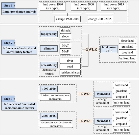
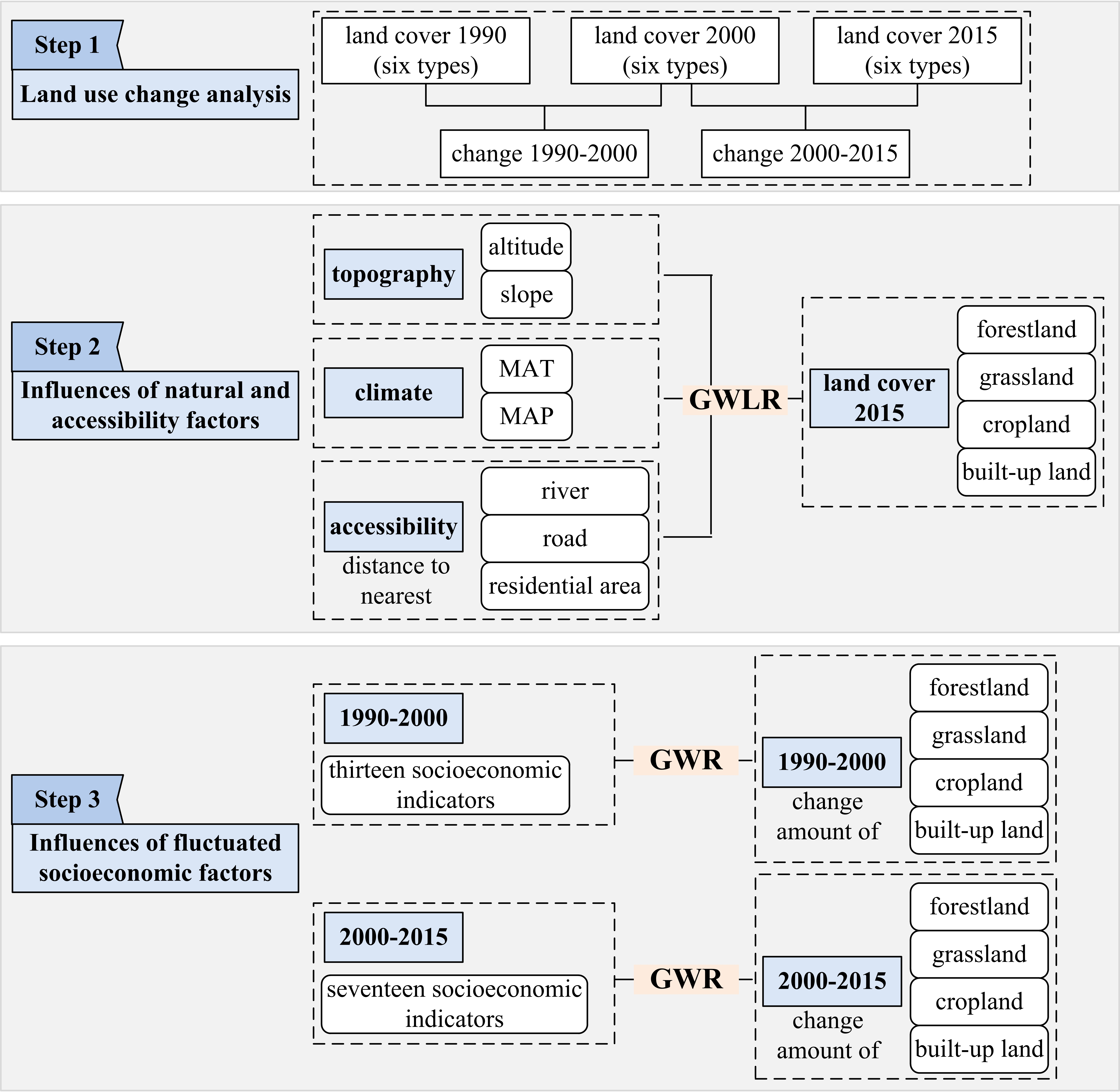
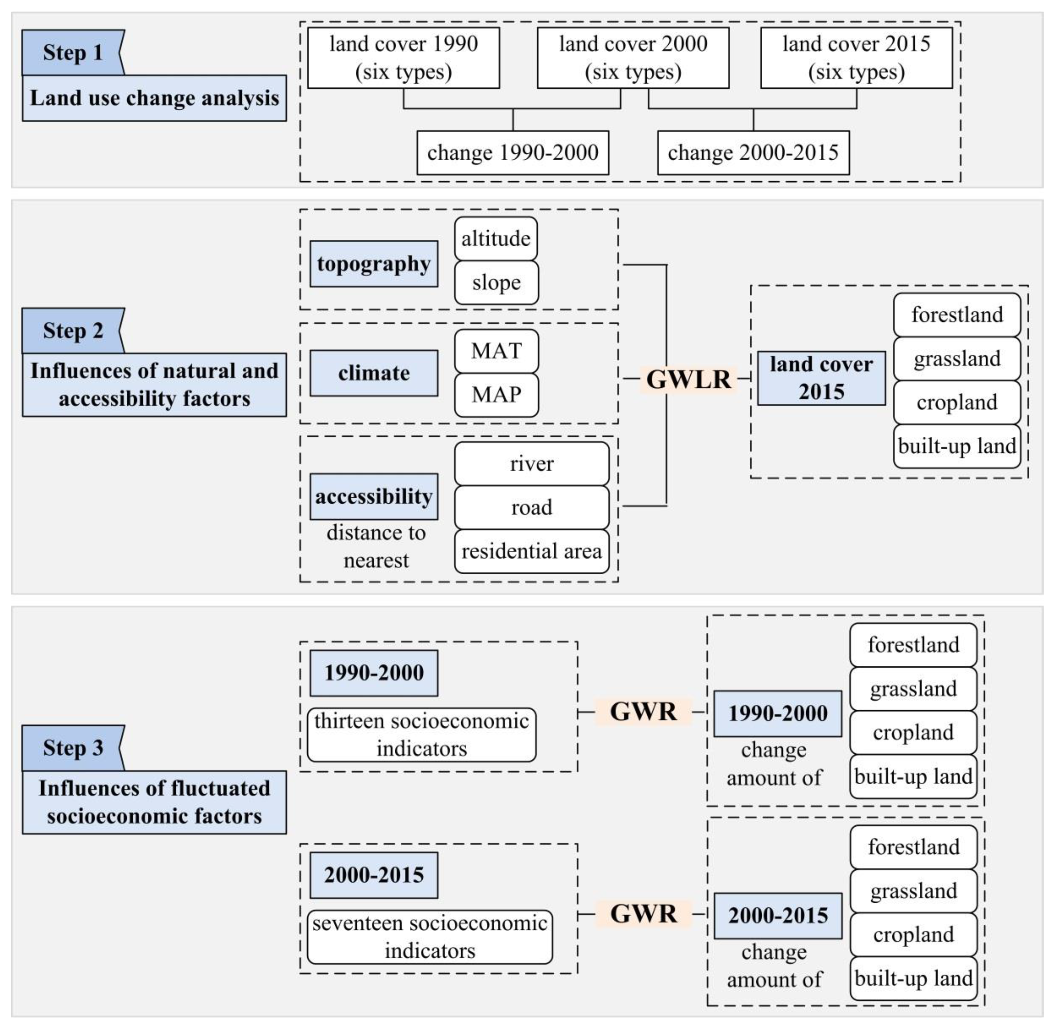
2. Materials and Methods
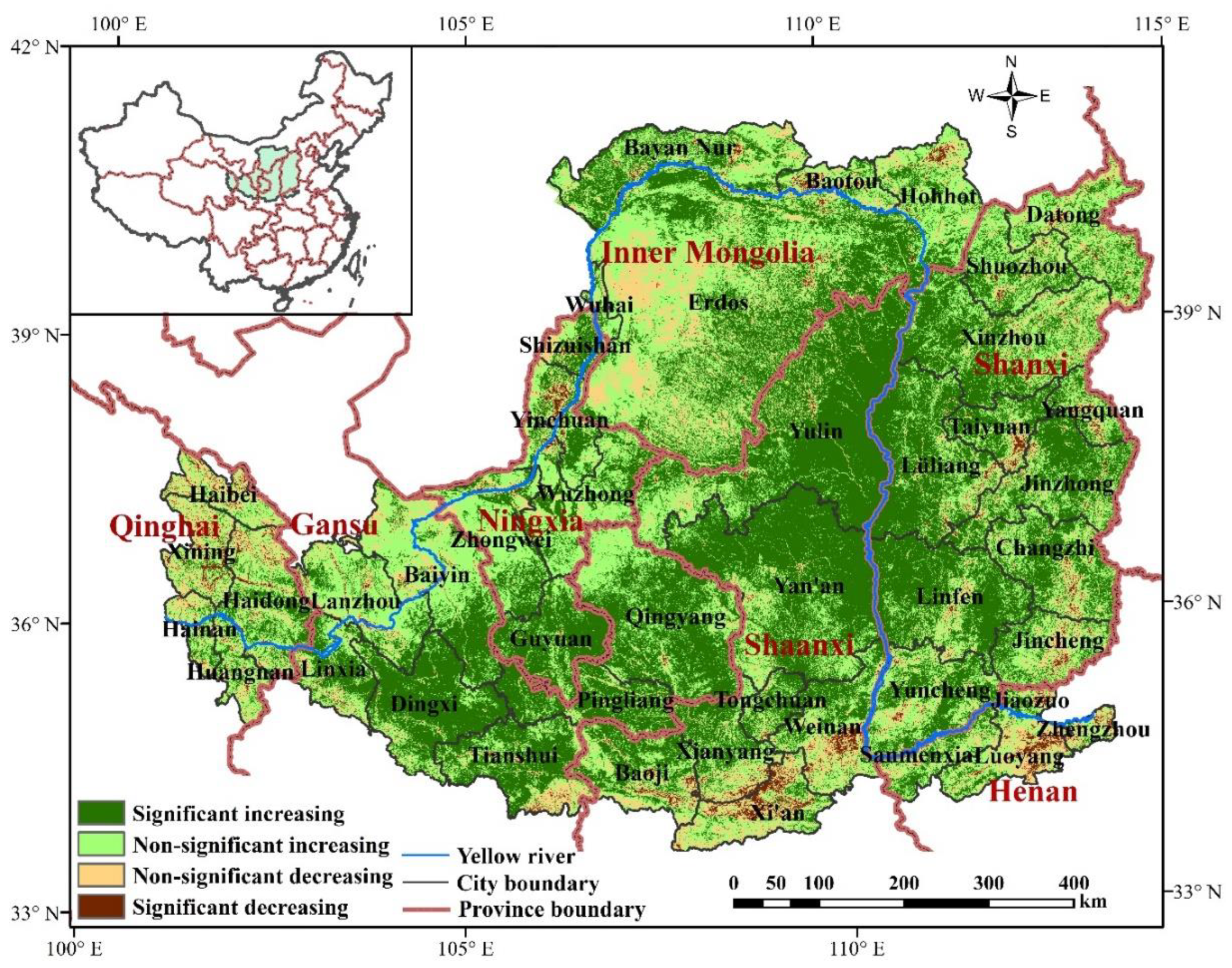
2.1. Study Area

The Loess Plateau (33°43′–41°16′ N, 100°54′–114°33′ E) is located in the middle reaches of the Yellow River basin in Northwestern China (Figure 1) and covers approximately 640,000 km2. The region is both the largest and deepest loess deposit in the world and is characterized by a temperate continental monsoon climate, with distinctly seasonal temperature and precipitation [32]. The annual average temperature is 4.3 °C in the northwestern region and 14.3 °C in the southeast. Most of the loess lies in a semiarid zone, with an average annual rainfall commonly less than 500 mm and chiefly concentrated in summer months, ranging from 250 mm in the northwest to 600 mm in the southeast [33]. Socioeconomically, Loess Plateau is a critical part of China’s great western development strategy and stands as a bridge linking western and eastern regional economies. It is distributed across 334 counties of 44 municipalities, belonging to seven provinces (i.e., Shanxi and most of Shaanxi and Gansu, as well as parts of Henan, Qinghai, Ningxia and Inner Mongolia) (Figure 1).
The Loess Plateau has become one of the most severely eroded areas in the world, with high soil-erosion rates and heavy river-sediment loads [10,33]. This is the result of human activity (e.g., agricultural development and urban sprawl) that has intensified over the past several decades, the erosion-prone soil, steep landscape, sparse vegetation cover and the high-intensity summer rainstorms. To address this environmental degradation, several ecological restoration projects have been implemented, including terracing, check-dam construction, reforestation and afforestation represented by the Grain-for-Green Program. Under this program, large areas of sloping farmland have been converted to forestland and grassland, leading to dramatic change of the land surface across the region (e.g., vegetation cover in Figure 1).

2.2. Data

2.2.1. Land-Cover Data

Land-cover maps of the Loess Plateau in 1990, 2000 and 2015 were derived from 30 m Landsat remote-sensing images. An object-oriented classification based on decision trees, combined with manual checks, was used for land-cover mapping. Field-measured land-cover types with GPS coordinates were collected to validate the land-cover maps, and the classification accuracy was about 94% [34,35,36]. The land covers were classified into six broad types: forestland, grassland, cropland, wetland, built-up land and other land (bare rock and desert) [37,38].
Land-use change analysis was carried out for the six types in two phases: 1990–2000 and 2000–2015, indicating the periods before and after the implementation of large-scale ecological restoration projects. Analysis of natural and socioeconomic driving factors included only four major land-use categories (forestland, grassland, cropland and built-up land), since the percentages of wetland and other land in the region were small and changes of these two types were negligible during the period.
A series of topographic, climatic, accessible and socioeconomic variables were selected according to the previous studies and data availability [16,19,39].

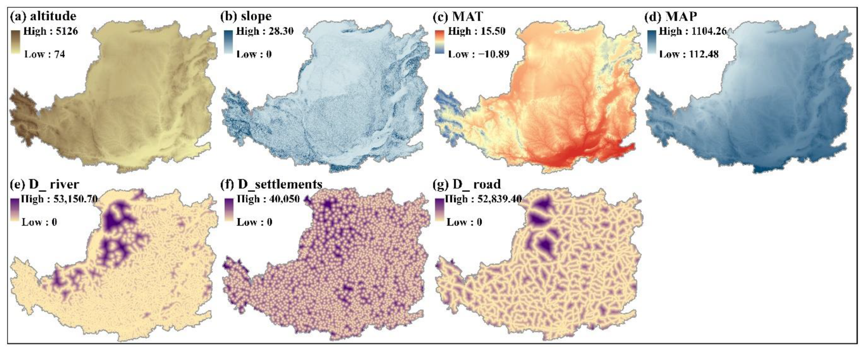
2.2.2. Topography, Climate and Accessibility Data

Altitude and slope were extracted from a 30 m resolution digital elevation model (DEM). Climate factors included mean annual temperature (MAT) and mean annual precipitation (MAP), which were calculated from the annual data from 1990 to 2015. Accessibility was calculated as distances to the nearest river, road and residential areas, with the features extracted from the 1:1M Geological Map Database of China. Table 1 summarizes the detailed information on the spatial datasets included in the analysis. Except for the NDVI, which was used for the trend analysis of vegetation coverage change in Figure 1, all the other data (i.e., land-use, altitude, slope, MAT, MAP, distance to the nearest river, distance to the nearest residential areas and distance to the nearest road) were resampled as a common regular 5 km grid, to facilitate the Geographically Weighted Logistic Regression (GWLR) for the limited calculation ability [40]. Binary logistic regression (IBM SPSS version 20) was used to create a parsimonious model by selecting variables with a significant contribution (p < 0.05) (Table S1) [19].

2.2.3. Socioeconomic Data

Socioeconomic data were obtained from statistical yearbooks and gathered at the county level. The area of afforestation was extracted from the China Forestry Database (http://www.forestry.gov.cn/), which provides a proxy reflecting the investment and contribution derived from ecological restoration projects. This was used because financial input data at the county scale may be incomplete or difficult to access. The dependent variables were calculated as the amount of change for the two periods (e.g., the percentage of forestland against county area in 2000 minus that in 1990). The same calculation was used for independent variables, except for the afforestation area, which was calculated as a cumulative value that the total area of afforestation during 2002–2014 divided by the county area. Thirteen driving factors were collected for the period 1990–2000 and seventeen for 2000–2015 (Table 2). A stepwise regression procedure (IBM SPSS version 20) was conducted to select the variables which add a significant contribution to the explanation of land-use change (Tables S2 and S3) [40].

2.3. Geographically Weighted Regression Method

GWR is an extension of ordinary least squares (OLS) global regression and generates local coefficient estimates to explore spatially varying relationships [27]. It constructs a series of local regressions by using data under a moving kernel that are weighted by their distance to the kernel center. The conventional GWR can be expressed formally as follows:
y i = β 0 ( u i , v i ) + k β k ( u i , v i ) x i k + ε i
where (ui, vi) is the coordinate of the ith location; yi, xik and εi represent, respectively, the dependent variable, the kth independent variable and the random error term at location i; and βk(ui, vi) denotes the local parameter estimate for kth independent variable at location i [41].
GW logistic regression (GWLR) combines the conventional GWR and the standard global-level logistic regression model. The standard global-level logistic regression suits situations where the dependent variables are binary and the goal is to determine the probability that a cell belongs to one class—in this case, a specific land-use type. GW logistic regression (GWLR) extends the standard logistic regression by allowing the coefficient of each independent variable to vary over space, stemming from the conventional GWR framework. It is described as follows:
L n ( P i 1 P i ) = β 0 ( u i , v i ) + k β k ( u i , v i ) x i k + ε i  
where L n ( P i 1 P i ) is the predicted odds for the ith observation, and Pi is the probability of forestland (or grassland, cropland and built-up land) covers at location i [42,43].
In this study, GW logistic regression was undertaken to analyze the influences of natural and distance factors on land-use spatial distribution at the grid-scale based on 2015 land-cover data. The dependent variables were binary; grids were assigned a value of 1 if they were occupied by forestland and value of 0 otherwise (the same was done for grassland, cropland and built-up land). Next, conventional GWR was conducted at the county scale for two periods (1990–2000 and 2000–2015), to explore the temporal and spatial effects of socioeconomic factors on land-use change. The dependent variable was the amount of change for one specific land-use type during the study period. This model was evaluated at the county scale, the most realistic level in light of data availability and administrative management activities.
Data processing and model-fitting were developed by using the following R software packages: GWmodel for GWR and GWLR modeling; sp, raster and rgdal for spatial-data manipulation (http://www.r-project.org). A critical parameter in any GWR is the bandwidth, which describes the size of the moving window by using a fixed distance or an adaptive distance based on the number of nearest-neighbor points considered for each local regression. Fixed bandwidths are typically used for regular gridded data, and adaptive bandwidths are used for irregularly distributed data. Two functions in the package GWmodel, bw.ggwr and bw.gwr, were used to automatically select the appropriate fixed and adaptive bandwidths for GWLR and GWR models, respectively [44]. Because all the data used in the GWLR and GWR models were standardized before the regression process, the coefficients of explanatory variables can be used to compare their relative contribution to the model fit [45,46]. Thus, for each model, we calculated the sum of the absolute value of each explanatory factor’s coefficients and identified the top four as the dominant factors to display spatially (the rest included in the Supplementary Materials: Figures S2 and S3). Figure 2 summarizes the analysis procedures.

3. Results

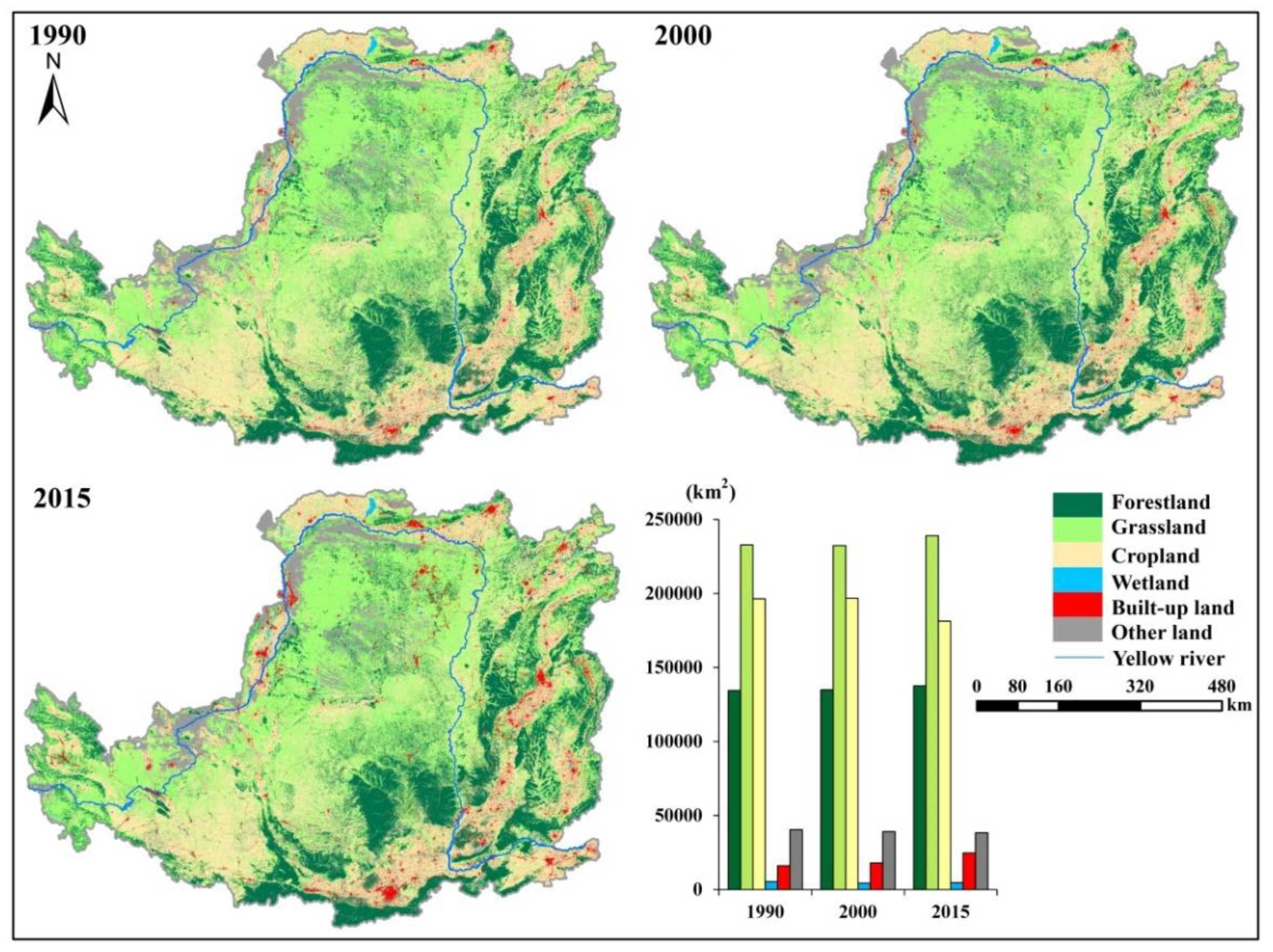
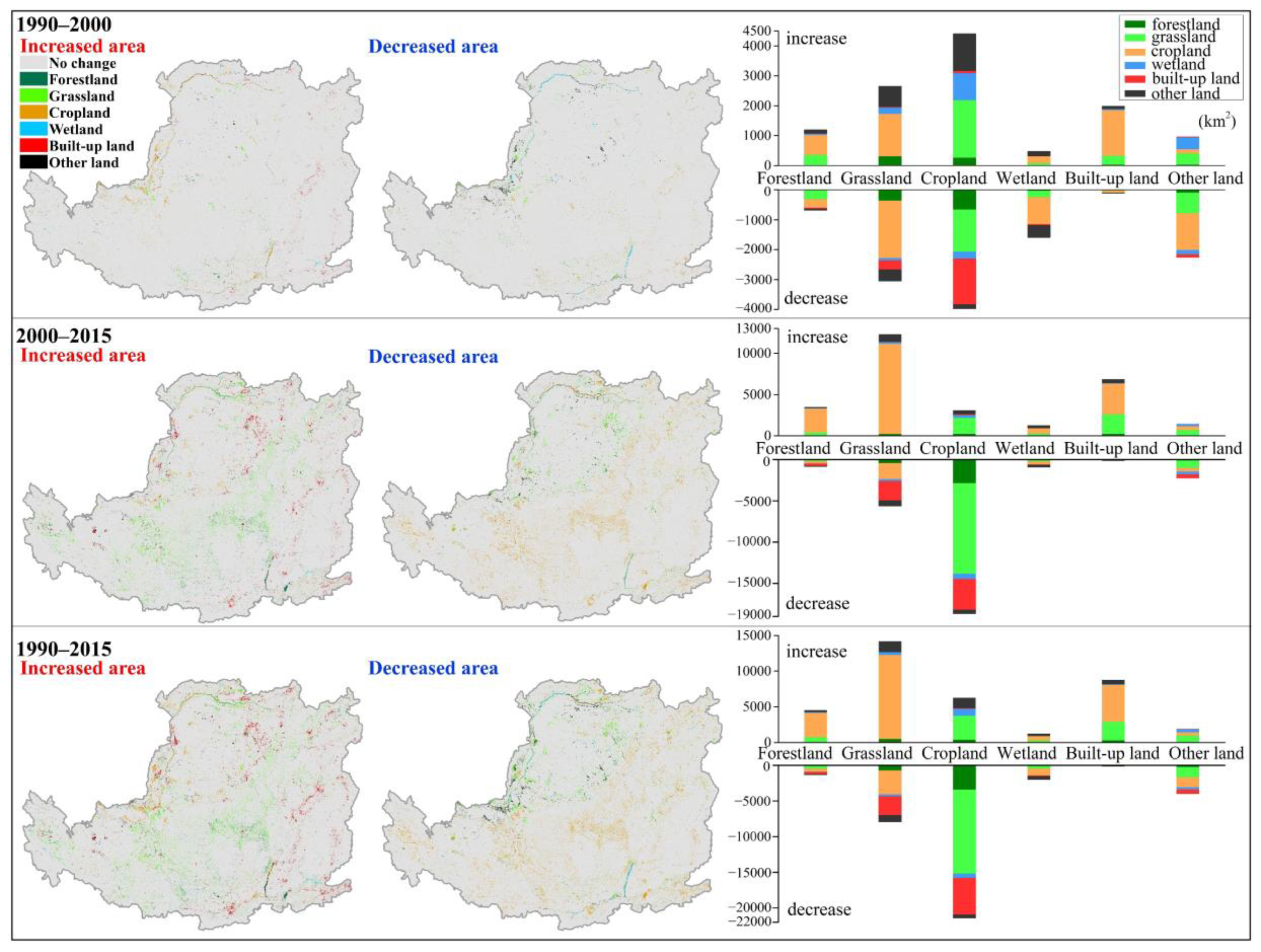
3.1. Land-Use and Land-Cover Change

Overall, the land-use structure in the Loess Plateau was relatively stable during 1990–2015 with grassland, cropland and forestland playing dominant roles, having a total area percent of about 88% (37%, 30% and 21%, respectively) (Figure 3). Nevertheless, this area also witnessed dramatic land-use transformations over the past several decades.
The land-use change displayed phased properties, with 2000 as a point of inflection. During 1990–2000, an area of 11671 km2 was subject to land change (Table S4) characterized by degraded grassland and wetland, expansion of cropland and built-up land, and weak restoration of forestland. In the period 2000–2015, greater land-use change was found (28,412 km2), with shrinking cropland and increasing grassland, built-up land, forestland and wetland. Land-use transformations also showed temporal variations (Figure 4). Grassland decreased by 0.17%, from 232,817 km2 in 1990 to 232,414 km2 in 2000, as a result of cropland expansion. Built-up land increased by 11.65% during 1990–2000, chiefly derived from cropland and grassland conversions. From 2000 to 2015, forestland, grassland and built-up land increased by 1.97%, 2.87% and 37.23%, respectively, with cropland as the main source (decreased by 7.9%).
Land-use changes not only show strong coupling and symmetry in change direction but also vary substantially over space (left panel in Figure 4). During 1990–2000, the increases in cropland occurred in the western region, the southern region and the borders of the northern region, co-located with decreasing grassland, bare land and wetland. Hotspots of built-up land gain included the east and north of the study area. During 2000–2015, the increases of forestland and grassland were notable in southwestern and central regions, concurrently with shrinking cropland. Built-up land also exhibited significant increases in this period though it accounts for a small fraction of the study area (less than 4%). Different land-use conversions were responsible for the expansion of built-up land across different areas. In the northern region, the increased built-up land was converted from grassland, whereas in the east and south, it came from cropland transformation. In summary, the region experienced pronounced land-use conversions from 1990 to 2015, characterized by forestland and grassland gain (ecological land restoration) in the central region, co-located with cropland loss and built-up land expansion in the eastern and northern areas.

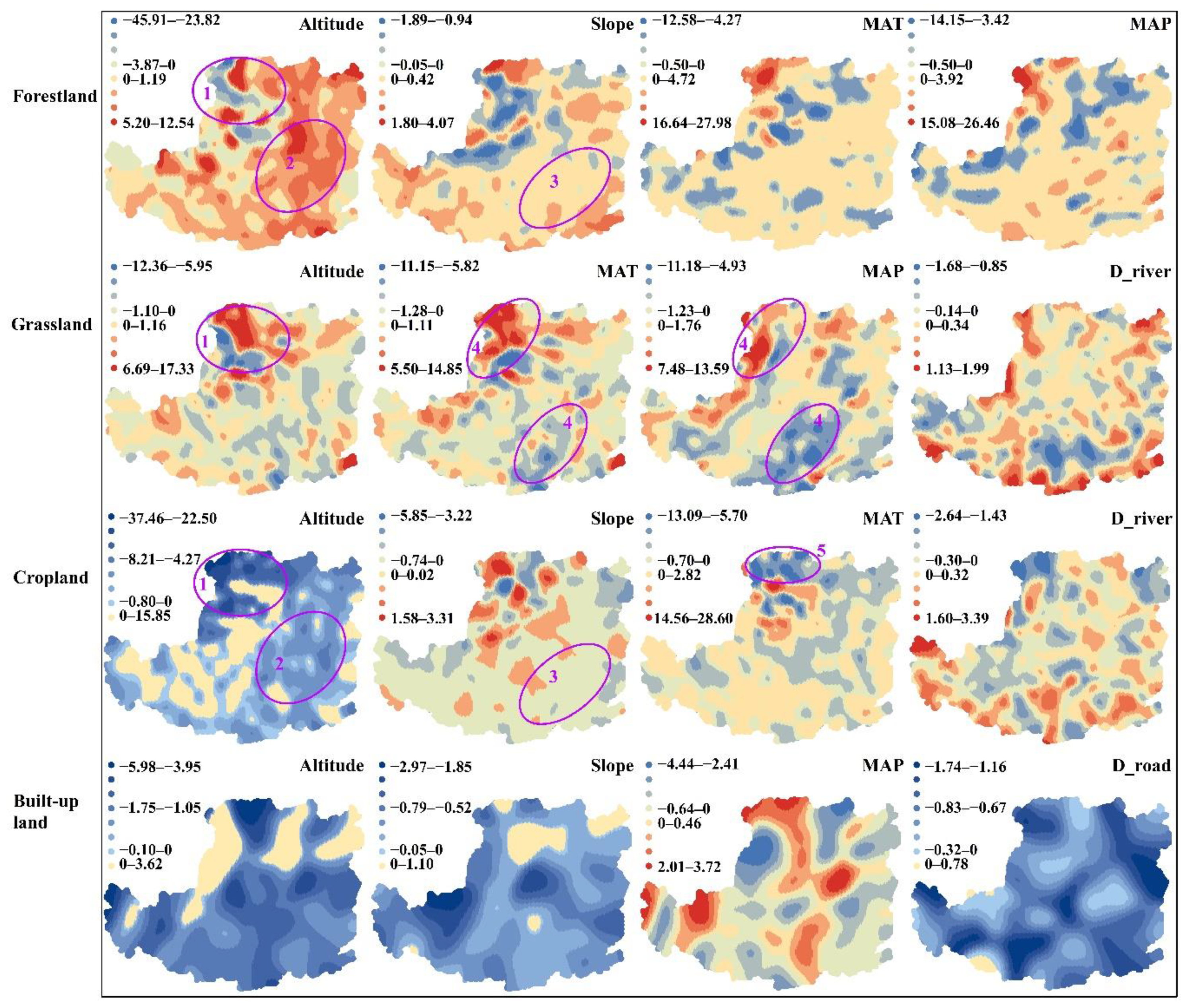
3.2. Internal Determinants of Land-Use Patterns Based on GWLR

The Loess Plateau is a diverse territory, with complex topography, climate and unevenly distributed artificial infrastructures (Figure 5). The region is dominated by hills and gullies, with the altitude and slope increasing from the northwest to southeast. The climate of the region displays significant spatial variations, expressed by the increases in mean annual temperature (MAT) and mean annual precipitation (MAP) from northwest to the southeast. The highest MAT occurs in the southern tip, and this part, as well as the Southern Shanxi province, has the highest MAP. Except for the Erdos, which is dominated by desert and the desert–steppe transition zone, the rest of the area has convenient transportation and is near rivers.
Four GWLR models corresponding to forestland, grassland, cropland and built-up land were constructed, and four dominant factors for each model were displayed spatially (Figure 6) (Table S5). The relationships between land-use distribution and the determinant factors exhibited spatially non-stationarity, indicated by varying spatial patterns of the GWLR parameter estimates. Altitude was the common dominant factor influencing the spatial patterns of the four land-use types, with varying intensities, represented by the different local coefficient ranges. Hotspots of the association of altitude with forestland, grassland and cropland were similarly distributed in flat northwestern regions (circle 1). Altitude exhibited a strong positive association with forestland, but a negative association with cropland in the central region, the key zone of soil erosion control projects (circle 2). The hotspots of effects of slope on forestland and cropland were also located in the northwest corner, displaying contrary signs across a large area in the central region (circle3). The associations of MAT and MAP with forestland varied in a similar manner across the whole study area, which may be related to the seasonal climate with concurrent rainfall and heat factors. Both MAT and MAP displayed positive associations with grassland in the northwest and negative associations in the southeast (circle 4). The hotspots of impacts of distance to river on grassland and cropland were concentrated in the border areas. In the cropland model, MAT showed a strong negative impact in the northwest (circle 5) and a weak (0–2.82) positive impact in the southeast. Except for MAP, which has a mix of positive and negative associations with built-up land, the other three dominant factors, i.e., altitude, slope and distance to road, all showed notably negative influences in large parts of the region, indicating that built-up land occurs in flat areas and near transportation infrastructures. The spatial variations of altitude and slope effects acted differently from that of the other three land-use types, and this may be due to the strong intrinsic dependence of built-up land to artificial shaping.

3.3. External Socioeconomic Drivers of Land Change Based on GWR

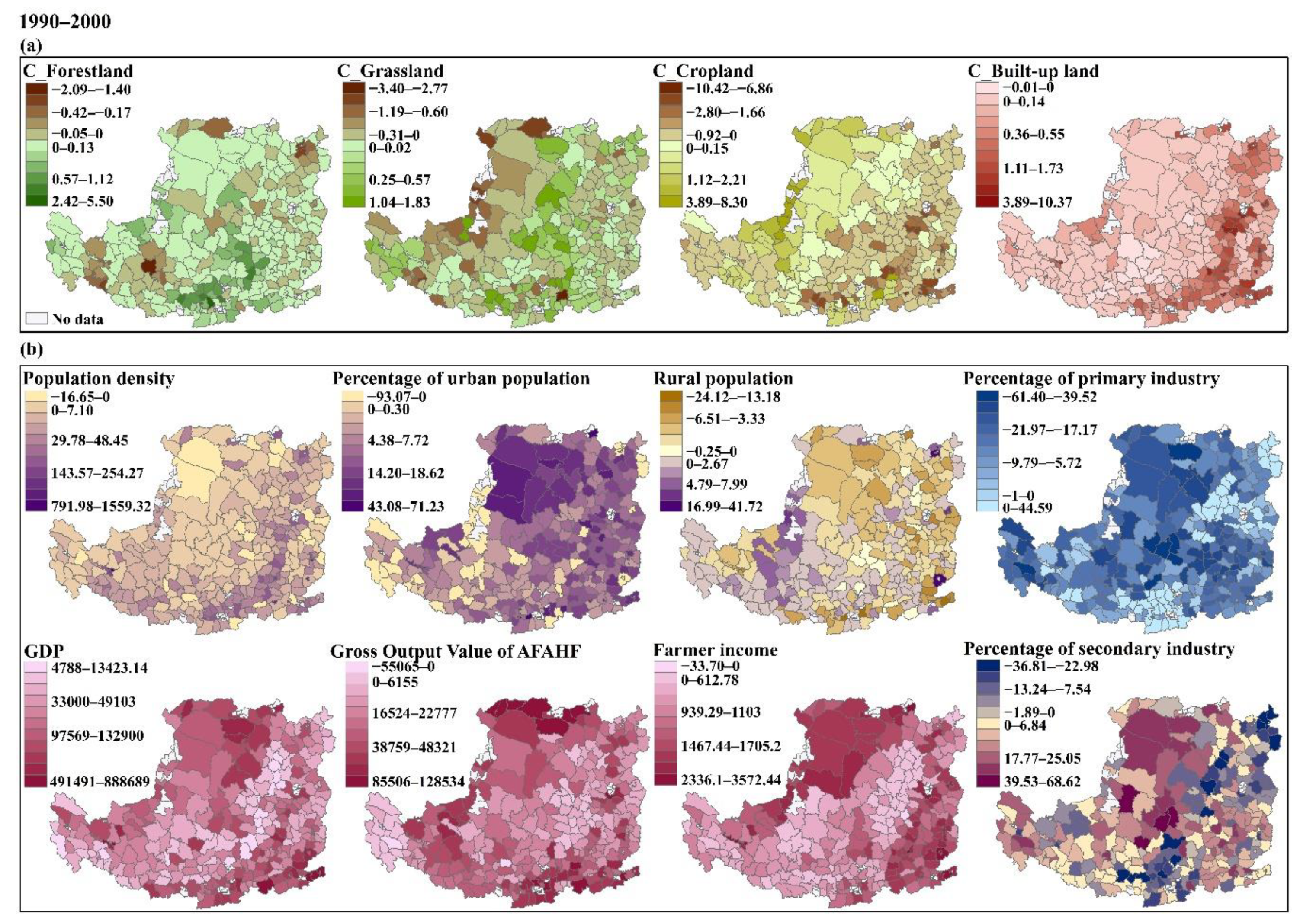
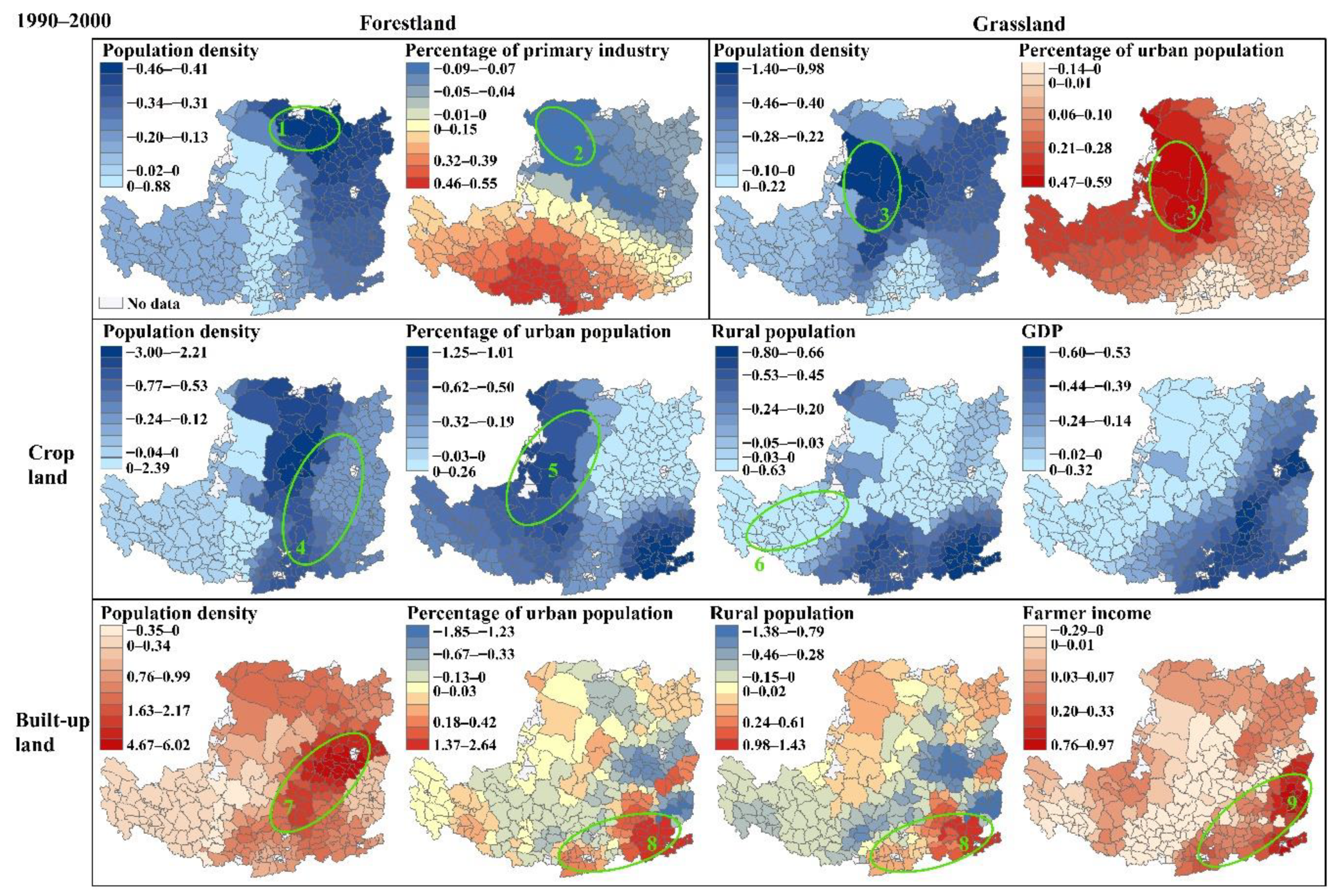
3.3.1. Driving Factors of Land Change during 1990–2000

During 1990–2000, the percentage of forestland area (against county area) in 69% of counties (196 out of 284 counties) increased, with a spatial concentration in the southern parts, and 49% of counties experienced grassland loss across the northwest (Figure 7a). The percentage of built-up land increased in 95% of counties, especially in the east, and 36% of counties experienced cropland gain, with hotspots in the northwest.
Figure 7b depicts the changes of multiple socioeconomic factors that were included in the four GWR models (Table S6). From 1990 to 2000, population density and percentage of urban population increased in most counties (93% and 88%, respectively), and 56% of counties experienced decreases in rural population, indicating the population urbanization trends, with concentrations in the northern and eastern areas. Industry structure has changed during this period, characterized by noticeable decreasing primary industry percent in the north, center and southeast, concurrently with increasing secondary industry percent. GDP (Gross Domestic Product) and Gross Output Value of AFAHF (i.e., agriculture, forestry, animal husbandry and fishery) increased across the region, most notably in the northern and southern extremities. A pronounced increasing trend of farmer income was found in the northern and eastern parts of the region.
Detailed summaries of the GWR models are in Table S6, and the impacts of the four dominant explanatory factors for each model were mapped spatially (Figure 8). The relationships between these factors and land change were spatially non-stationary, with clear spatial patterns in the distribution of the GWR model parameter estimates. First, in the forestland model, changes in population density and the percentage of primary industry were strongly associated with changes in the percentage of forestland, with a noticeable mix of positive and negative impacts. The strongest negative impact of increased population density can be found in a group of counties in the north (circle 1), co-located with forestland gain. The percentage of primary industry inflected from a positive association in the southwest to a negative one in the northeast. A hotspot was found in the northwest (circle 2), indicating that decreased primary industry percent had a notable negative impact on the forestland gain. Secondly, in the grassland model, population density and percentage of the urban population were the only two explanatory factors that remained after the initial selection process. In the central and western regions (circle 3), weak increases in population density (0–7.1) were strongly negatively associated with grassland loss, while increases in urban population percent showed a hotspot of positive impact.
In the cropland model, increases in population density were strongly negatively associated with the cropland loss in the eastern region (circle 4). In the northern part, increases in urban population percent showed negative associations with cropland gain (circle 5). In the southwest region, increases in the rural population were positively associated with cropland gain (circle 6). Increases in GDP were associated positively with cropland gain in the northwest and negatively with cropland loss in the southeast, indicating a consistent accelerating effect of GDP on cropland. The pronounced increases in built-up land were correlated with changes in population density, percentage of urban population, rural population and farmer income. Increases in population density across the region were positively associated with built-up land gain, with hotspots in the southeastern part (circle 7). Urban population percent and rural population had similar spatial patterns of associations with built-up land gain, with a positive impact hotspot in the southeast corner, surrounding the large cities (circle 8). This indicates that increases in urban population percent and decreases in rural population accelerated the built-up land expansion in these areas. This part also shared a hotspot of the positive impact of the increased farmer income (circle 9).

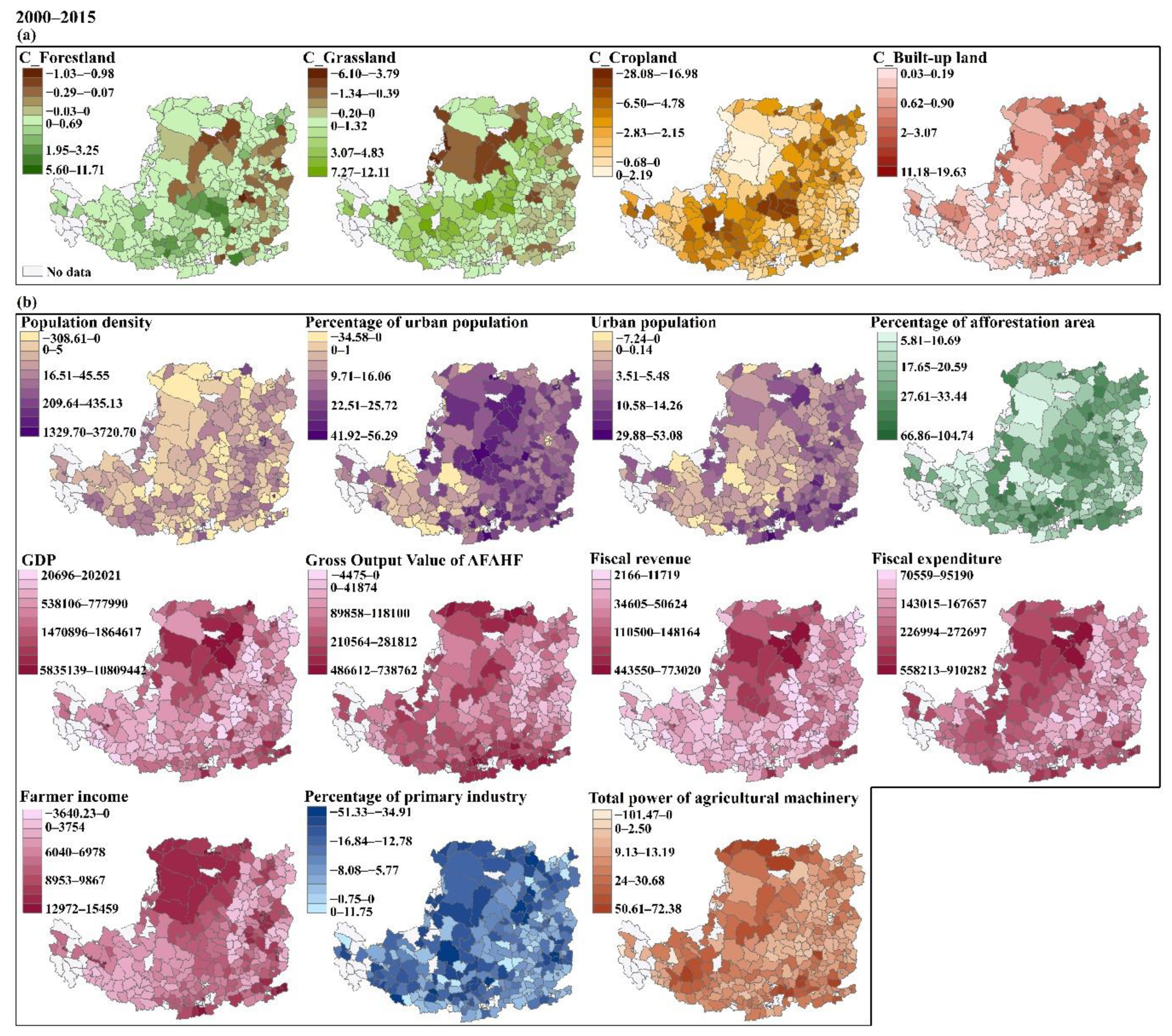
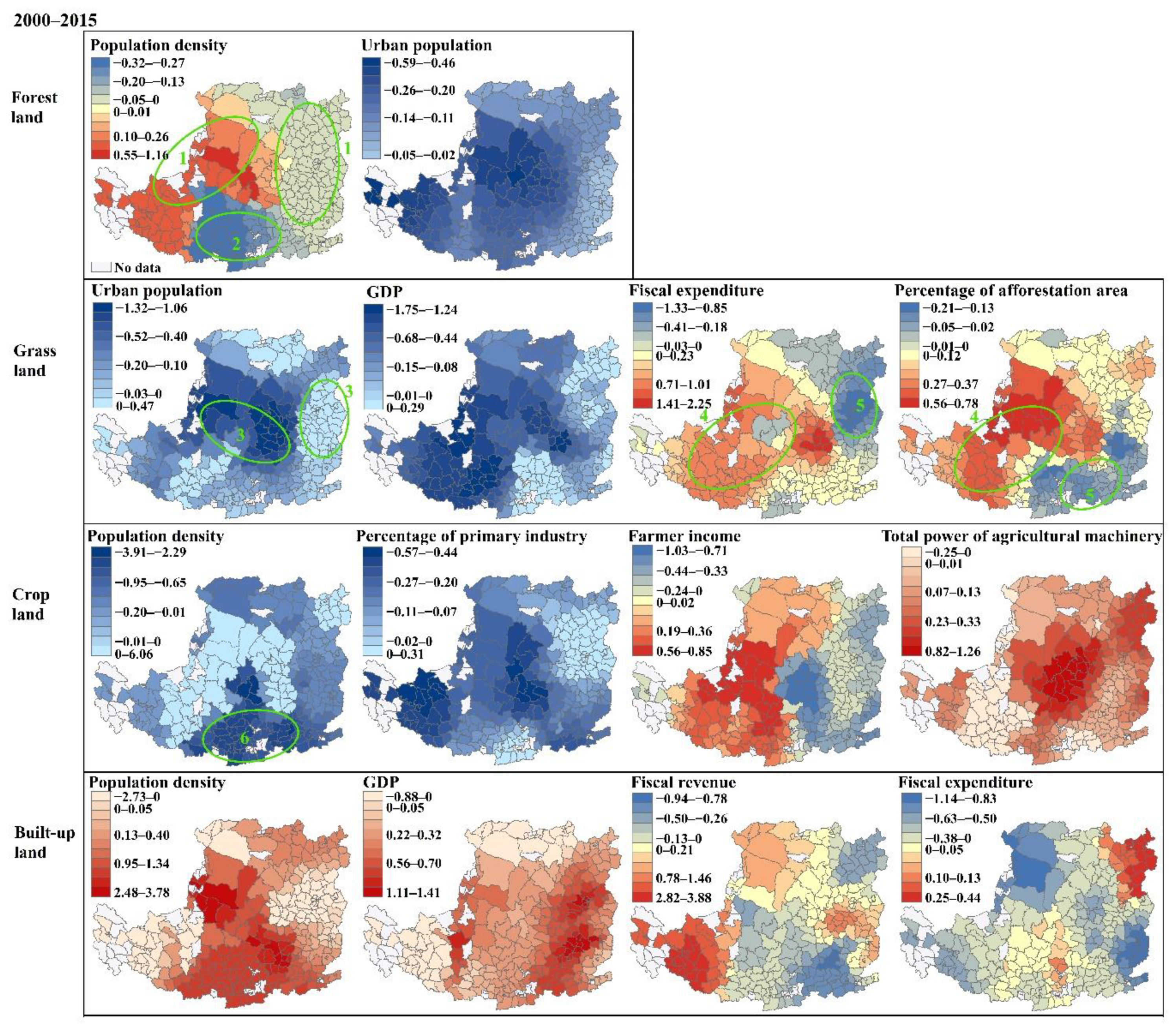
3.3.2. Driving Factors of Land Change during 2000–2015

During 2000–2015, most counties experienced forestland and grassland gains, with 76% and 69% (218 and 198 out of 288 counties), respectively, spatially clustered in the central and western parts of the region (Figure 9a). The percentage of cropland decreased in almost all counties (97%), co-located with gains in forestland and grassland. Built-up land expansion occurred in all counties, especially in the northeastern regions.
Compared with the earlier period (1990–2000), the increasing trend of population in this period is weaker with 82% (235 out of 288) of counties experiencing increased population density (Figure 9b). The magnitude and percentage of urban population in most counties (92% and 87%, respectively) increased, with hotspots in the northern and southeastern regions. A range of economic indicators, including the GDP, gross output of AFAHF, fiscal revenue, fiscal expenditure and farmer income, were found to increase in all the counties (above 99%), especially in the northern region and southern extremities. The percentage of primary industry decreased across a large area of the region, including 93% of counties mostly located in the north and west. Some 92% of counties experienced overall increases in the total power of agricultural machinery. Peak values for the cumulative percentage of afforestation area were found in the central and western regions, which is the key zone of multiple ecological restoration programs.
Detailed results of GWR model outputs are summarized in Table S7, and the spatial variation in coefficient estimates of the dominant factors are shown in Figure 10. First, population density experienced the transition from a positive association with forestland gain in the west to a negative one with forestland loss in the east (circle 1). Moreover, population density appeared to have a strong negative impact in a small part of the south which has experienced notable forestland gain (circle 2), potentially originating from the mixed signs of population density change in this part. Increases in urban population were negatively associated with forestland change, with intensity decreasing from west to east. Second, grassland change was correlated with the urban population, GDP, fiscal expenditure and cumulative percentage of afforestation area. The urban population showed a strong negative association with grassland gain in the central region but positively associated with grassland loss in the east (circle 3). The impacts of GDP acted in a similar manner as the urban population and showed negative influences across a larger area in the western region. Both hotspots of the positive impacts of fiscal expenditure and afforestation area percent were located in the center and southwest (circle 4), where grassland increased; meanwhile, in the eastern parts that experienced grassland loss, the two factors showed a negative impact, with hotspots in the northeastern and southeastern corners, respectively (circle 5).
The four dominant factors for cropland included population density, percentage of primary industry, farmer income and total power of agricultural machinery. Population density displayed a negative association with cropland loss, especially in the southeast (circle 6). In the central and western regions, decreases in primary industry percent showed a strong negative association with cropland loss. The influence of increased farmer income on decreasing cropland shifted from positive in the west to negative in the east. Increases in the total power of agricultural machinery showed a consistently positive association with the cropland loss, with hotspots in the central region. Population density, GDP, fiscal revenue and fiscal expenditure dominantly influenced built-up land expansion from 2000 to 2015. Population density and GDP both showed strong positive associations with the built-up land gain across a large area of the region, with hotspots in the central and eastern regions, respectively. The impacts of increased fiscal revenue and expenditure showed complex and contrary spatial patterns.

4. Discussion

4.1. Land Degradation and Restoration in the Semiarid Loess Plateau

As a result of the policy “Take Grain as the Key Link,” which was started in the 1950s, the population of the Loess Plateau rose sharply, stimulating a large increase in the area of sloping farmland and the reduction in forestland and permanent grassland, leading to severe soil erosion and degraded ecosystems [10,47]. To control soil erosion and restore the environment, the government has undertaken a series of engineering works since the late 1960s, including the construction of check dams, terraces and reservoirs [48]. However, vegetation cover did not systematically increase until 1999, and this can be attributed to the region’s drying climate [49]. A comprehensive analysis conducted in the arid and semiarid zones of China showed that forestland and grassland had net losses, while farmland and built-up land had net increases in the area during 1990–2010 [50]. This study also qualitatively indicated the agricultural encroachment to be the primary driver of the loss of natural ecosystems, with the continuous impact of built-up land expansion. In the present study, we used the most direct land-cover change to reflect the land transition processes in the semiarid Loess Plateau, and the results show that grassland degraded by 0.17%; forestland and cropland increased by 0.38% and 0.22%, respectively, during 1990–2000. This indicated that cropland continued to expand and grassland to degrade, despite the restoration of forestland in this period under the restoration initiatives. The analysis of driving factors revealed that demographic factors, especially population density and urban population percent, were the common dominant factors associated with the changes of four major land-use types, including forestland, grassland, cropland and built-up land. In 1999, the largest global re-vegetation program, Grain-for-Green, was initiated nationally and the Loess Plateau was included as a key zone. Numerous studies have reported the significant increasing trend of vegetation coverage in the Loess Plateau benefiting from the program [51]. In our study, forestland and grassland were found to increase by 1.97% and 2.87%, respectively, from 2000 to 2015, concurrently with cropland decreasing by 7.9%, as a result of the policy-motivated land restoration.
Post hoc assessment is a core component in the cycle of program implementation. A variety of assessments on the effectiveness of ecological restoration projects have been carried out across the world at a range of scales [52,53]. Lü et al. (2015) compared the effects of three large-scale ecological programs (National Nature Reserves, Three North Shelter Forest Program and the Natural Forest Protection Program) on Chinese vegetation change and revealed that the effectiveness of ecological restoration projects can vary geographically, even under the same incentive policy context [54]. Various local socioeconomic conditions may be responsible for this. The present regional-scale study confirmed this finding and further characterized the spatial variations of the impact of ecological restoration efforts across the Loess Plateau, with the positive (amplifying) hotspots located in the central and southwestern areas. Varying from previous studies which merely focus the restoration progress on the projects themselves, our results identified the positive associations of farmer income and total power of agricultural machinery on cropland loss (fewer disturbances and more potential for natural ecosystems) in the western parts and across the whole region, respectively. This indirectly reflects the positive roles of agricultural improvements and higher rural economic welfare in the vegetation restoration.

4.2. Better Performance of GW Method Compared with Global-Level Models

Most previous studies have neglected the regional variability of economic and policy influences on the land system, which are difficult to quantify [19]. Additionally, several studies lack information on socioeconomic drivers over time [55]. These have become an obstacle for constructing quantitative models of impacts of different drivers, consequently hindering further land-change research. This study focused on the land-change processes in a typical dryland region from both spatial and temporal perspectives and has suggested how causal associations with multiple biophysical and socioeconomic forces and their variations could be quantified. In this study, even though the R2 of both the GW methods and the global-level non-spatial regression were not too high, the GW methods yielded better model fits, as is indicated by lower AICc values and higher R2 (Pseudo R2 of logistic regression and adjusted R2 of conventional regression) (Table 3). This is in line with the findings of An et al. (2016) and Rodrigues et al. (2014) [25,56]. Our analysis confirms that GW methods support further investigation and a deeper understanding of the complex relationships between land change and the underlying driving forces. GW methods can reveal the detailed site information on the different roles of the driving forces in different regional parts [57]. In addition to spatial variation, this research also provided evidence that the effect and magnitude of these driving forces change over time.
The results from the GWLR and GWR models revealed detailed local information on the different roles of factors in relation to the land change across the study area. In the GWLR models, natural and accessibility factors act as foundations, providing the possibility for the presence of different land-cover types. Each location has specific topography and climatic conditions that determine the potential of natural and agricultural vegetation. Our results showed that altitude was the common dominant factor for the four major land-use types. In the high, steep central region, both altitude and slope were positively associated with forestland, while negative associations were found with cropland, which reflects the theoretical basis of the Grain-for-Green program that converts sloping farmland to forestland and grassland, in order to control the serious soil erosion. MAT and MAP were found to behave in a similar manner in relation to forestland and grassland distributions, with positive hotspots in the ecologically fragile and rain-heat limited northwest. Biophysical conditions are also important for the suitability of a location for residential construction. Altitude and slope showed a negative impact on built-up land across most parts of the region. It needs considerable investment to reclaim high, steep land for residential demands, and thus preferences will exist to direct the developments to better-suited locations with lower construction costs [15]. The pronounced negative associations of distance to road with built-up land across almost the whole region emphasized the increasing importance of traffic connections for urban development [58].
Changing economic conditions and shifting societal needs drive and shape landscapes and attendant land-cover changes. In the GWR models, for the period 1990–2000, in the central and western regions, increased population density accelerated forestland, cropland and built-up land gain and hindered grassland deterioration, indicating that a higher population accompanied higher demands for land, crops and natural resources. In this area, increased urban population percent displayed a positive association with grassland degradation and a negative association with cropland gain which may be related to sharp decreases in labor dedicated to agricultural activities. GDP showed consistently accelerating impacts on cropland, locally expressed by a positive association with cropland gain in the northwest and a negative one with cropland loss in the southeast. Notably, in the southeast corner, increased farmer income showed strong positive associations with built-up land gain, resulting from higher affordable ability and residential demands. In the later period (2000–2015), in the southern region, increased population density showed negative associations with forestland gain and cropland loss, while being positively associated with built-up land expansion. Increased urban population hindered the forestland and grassland gains, indicating a threat to the vegetation restoration. In many studies, policies are not given explicit attention because they are difficult to include in a quantitative manner [15]. In this study, fiscal expenditure and afforestation area percent, as proxies for national policies and investments, both showed strong positive associations with grassland gain across a large area in the center and west, the key zone of ecological construction projects. This, in some sense, reflected the initial success of the ecological restoration measures in these areas. However, GDP showed negative influences in the same area. Increased farmer income and total power of agricultural machinery implied a positive impact on cropland decreasing in this part. Increases in farmer income mostly come from off-farm activities, e.g., rural labor emigration, simultaneously decreasing the farmer’s willingness to engage with traditional cultivation. Moreover, less labor was needed for the same cultivation activities, as a result of technological evolution and intensive management of cropland.
Overall, ecological restoration projects effectively contributed to the greening trend of the region (especially grassland in this study), with hotspots spatially clustered in the center and west. This is consistent with the previous studies [59,60,61]. Our results also identified restoration progress in the target of improving farmer well-being, expressed in the strong positive impacts of increased farmer income on built-up land expansion in large cities of the southeast, and the accelerating effects on cropland decrease accompanied with improved agricultural machinery. However, in the areas where forestland and grassland had changed significantly (central and western regions for 1990–2000, and the southern region for 2000–2015), urban population characteristics showed undesired effects, expressed in accelerating grassland degradation in the first period and hindering forestland and grassland restoration in the later period. This deserves special attention in future restoration strategies, in order to realize effective and sustainable land management.

4.3. Implications for Land-Change Modeling and Land Management

Quantifying the relationships between land change and the hidden possible causes is a key step in land-change research [17,18]. By exploring the spatiotemporal characteristics of land-change processes and the driving-force mechanism, land-use-change models can be formulated to simulate future changes [16]. Traditional land-change modeling has been almost completely based on the global-level logistic regression [62], which does not effectively capture the non-stationary processes and factors associated with the land in reality. In this regard, the location-dependent statistical relationships we proposed can be used to improve the performance of regional land-use change models and to evaluate the consequent impacts on the ecological environment, e.g., the projected ecosystem services [13]. For example, incorporating GWLR-derived spatially varying relationships within cellular automata (CA) models to simulate rapid urban growth can fully address local relations in the land-change processes and improve the overall modeling accuracy [63]. Other applications include the introduction of GWR concepts in the transformation rules of CA to project future developments in urban ecological security, and modifying the traditional CLUE-S model with GW approaches to simulate the regional land-use change [64,65]. The local statistical relationships identified by the GW models, as well as future projections, can contribute to context-related land management and proactive policy-making [66].
Balancing urbanization and ecological restoration is critical for land management. Huang et al. (2020) used the GWR methods to systematically analyze the spatiotemporal characteristics and driving forces of land-development intensity in Western China during 2000–2015, and they found that investment intensity significantly promoted land development intensity, while the natural and ecological environment distinctly constrained the development [67]. As for the Loess Plateau, Wang et al. (2018) have quantified the magnitude of the impacts of climate change, urban expansion and the Grain-for-Green Program on land-use change during 1980–2015, and the results showed that the three factors accounted for 93.65%, 5.46% and 0.64% of the total, respectively [68]. The present study focused on the spatiotemporal variations of the impacts of driving factors on land-use change in the Loess Plateau. The findings make it clear that policy-makers need to be aware of the spatiotemporal processes of land change. The shifts in land-change drivers during the two periods imply that effective land management requires shifts in policy over time and adapted strategies to fit new temporal and regional demands. By quantifying the local statistical relationships, we hope to provide land managers with a blueprint to start disentangling the role of major land-system drivers. For example, our results indicated the continual stress of urban population characteristics on the Loess Plateau’s vegetation retention, expressed in promoting grassland degradation in the center–west during 1990–2000 and hindering forestland and grassland restoration in the south during 2000–2015. The identified stress of urban population on regional vegetation, combined with the previously reported conflicting water demands between ecosystems and humans [69], makes it essential to pay special attention to the post-maintenance and protection of restored vegetation, especially in the key center–west and south parts of the region. Numerous studies have argued that vegetation in the Loess Plateau should be maintained but not expanded further, due to the limited water capacity and mitigating food deficit [47]. The inherent water-limited physical characteristics, mismanagement of planted vegetation (e.g., introducing exotic plant species and high-density planting), greater water demand induced by the increased urban population and the expansion of industrial activities generated substantial new challenges for protecting the ecologically sensitive regional environment. Alleviating human pressures on ecosystems is inevitably a critical task for ecological restoration initiatives [54]. For example, infrastructure construction, e.g., railways and expressways and other urbanization industrial activities, should minimize their influences on the environment (e.g., biodiversity and the water footprint). Large-scale phased assessments of land-change processes and long-term monitoring efforts are continually needed in order to realize long-term sustainable ecological restoration progress.
More importance should be attached to agricultural improvements and higher rural economic welfare. Our results show the improvements in farmer well-being, expressed in the strong positive associations of increased farmer income, with built-up land expansion in the southeast, and its accelerating effects on cropland conversion to natural ecosystems, accompanied by improved agricultural machinery. In the future restoration, more research on vegetation management and increases in agricultural efficiency, while avoiding farmland expansion through deforestation, are needed to reduce water uptake by vegetation, to ameliorate water shortages on land used for food production, and therefore mitigate the abovementioned conflicting water demands. In addition, rural human welfare should be further enhanced. Currently, farmers receive greater economic incentives to participate in the Grain-for-Green program than to grow food on their land [47]. More government incentives should be invested to improve the level of rural economic development and residential welfare (e.g., more technological support for agricultural production and the diversification of farmer income), which can play positive roles in ecological restoration and synchronously decrease the risk of undesired land degradation resulting from rural poverty and land reclamation [70].

4.4. Caveats and Ways Ahead

Even though detailed insights into the land-change process are provided, there are additional aspects that the present analysis did not address. The specific land-change drivers are diverse and location-dependent [15,62,71,72], which can be preliminarily characterized by the GW methods and visualized spatially according to a series of local parameters. Nonetheless, it is difficult to interpret the model outputs thoroughly, an issue which is also encountered in our study, considering that the demand of decision makers to get appropriate and intuitionistic understanding of the results is high. A potential solution is to cluster or zone the parameter surfaces with the help of extensive regionalization algorithms, and thus reducing the complexity of the model outputs [19,73]. This is also a way for future additional investigations of geographical relations in order to reach full potential of the GW methods.
Human societies constantly interact with the environment through mutual feedbacks and adaptations [74]. The land-change drivers are interactive, and the links between land change and several driving forces may be bidirectional. For example, socioeconomic conditions and policy shift may influence stakeholders’ choices and allocation of the land resources [75], and thus lead to changes of the land surface. Subsequently, the changed land structure can contribute to regional economic development in the next stage in various aspects, e.g., industry structure and household income [76]. However, the two-way interconnections were not included in the scope of this study. Our focus here was to quantify the spatiotemporal variations of the impacts of physical and socioeconomic factors on the regional land change. To date, a few attempts have been made to explore the complex connections and feedback among the human–environment system, mostly based on the coupled land-change models and limited to non-spatial analysis [77,78,79]. Further research to nest local statistical relationships in the studies of human–environment interactions is still ongoing.
In the present study, analyses of natural and accessibility factors were conducted in the grid-scale, and influences of socioeconomic forces were based on the administrative county-level, conditioned by the data availability. By using several innovative geographical analyses (e.g., interpolation), several studies have tried to convert the administrative-unit-based socioeconomic data to regular grid-cell maps [24]. This conversion provides the potential to combine natural (especially the annual temperature and precipitation) and socioeconomic influences in land-change research. Moreover, this can result in higher goodness-of-fit for its concerns of the heterogeneity within a single administrative unit. The conversion is based on the premise of enough statistics underpinning the interpolation or rasterization. Continuing land-use change and the critical role of socioeconomic factors in modifying land cover warrants extensive monitoring and compilation of the socioeconomic statistics, a notable limitation of the present socioecological-system research [40,80].

5. Conclusions

In this work, we explored the driving forces behind land change in the Loess Plateau, China, one ecologically fragile and typical dryland region in the world. We made new attempts to at least partially fill in the knowledge gaps in land-change science by comprehensively investigating land-change processes (i.e., land degradation and restoration) and the spatiotemporal variations in underlying natural and socioeconomic driving forces, by utilizing local GWLR and GWR models. Overall, this study comes to three main conclusions: The Loess Plateau has experienced dramatic land-use transitions over the past twenty-five years, with 2000 as a turning point displaying phased changes in features; the influences of the natural and accessibility factors on land-use distribution exhibited spatially non-stationarity, implying the variable potential and suitability of different land-use types; the relationships between land-use changes and different socioeconomic factors were found to vary over space and time, highlighting the adaptive land management and timely policy responses.
Quantifying process spatial heterogeneity through a GWR framework provided a higher level of explanation of the relationships between land change and related factors, which can inform improvements in land-change-model performance through the inclusion of more representative measures of causality. Results of the study also indicate the importance of striking balances between urbanization and ecological restoration, and the enhancement of agricultural development and rural welfare. This is a suitable starting point to disentangle the complex relations in the land-change processes and to provide scientific evidence in support of context-aware land management in dryland areas, with the aim to harmonize human–environment relationships and to achieve the target of a land-degradation-neutral world.

Supplementary Materials

The following are available online at https://www.mdpi.com/2072-4292/12/3/453/s1. Figure S1. Major ecological restoration programs under implementation in China. Figure S2. Estimation of GW Logistic Regression coefficients for the remaining explanatory factors. Figure S3. Estimation of GWR coefficients for the remaining explanatory factors. Table S1. Selection of topographic, climatic and accessible variables for the forestland, grassland, cropland and built-up land models. Table S2. Selection of socioeconomic factors for the period 1990–2000. Table S3. Selection of socioeconomic factors for the period 2000–2015. Table S4. Transition of area from 1990 to 2000 (a), 2000–2015 (b) and 1990–2015 (c) (km2). Table S5. Explanatory factors and the summary statistics of their varying (local) coefficients in the GWLR models. Table S6. Explanatory factors and the summary statistics of their varying (local) coefficients in the GWR models (1990–2000), Table S7. Explanatory factors and the summary statistics of their varying (local) coefficients in the GWR models (2000–2015).

Author Contributions

Conceptualization, Y.R. and Y.L.; data curation, T.L. and J.H.; formal analysis, Y.R.; funding acquisition, Y.L.; methodology, Y.R.; writing—original draft, Y.R.; writing—review and editing, Y.L., B.F. and A.C. All authors have read and agreed to the published version of the manuscript.

Funding

This research was funded by the National Key Research and Development Program of China [No. 2016YFC0501601], the Strategic Priority Research Program of the Chinese Academy of Sciences [No. XDA23070201], and UK Research and Innovation [NE/S009124/1].

Acknowledgments

Thanks also go to Liyang Ma for the help with the initial data collection.

Conflicts of Interest

The authors declare no conflicts of interest.

References

  1. Verburg, P.H.; Crossman, N.; Ellis, E.C.; Heinimann, A.; Hostert, P.; Mertz, O.; Nagendra, H.; Sikor, T.; Erb, K.H.; Golubiewski, N.; et al. Land system science and sustainable development of the earth system: A global land project perspective. Anthropocene 2015, 12, 29–41. [Google Scholar] [CrossRef] [Green Version]
  2. GLP. Global Land Project. Science Plan and Implementation Strategy; IGBP Report No. 53/IHDP Report No. 19; IGBP Secretariat: Stockholm, Sweden, 2005; 64p. [Google Scholar]
  3. Uhrqvist, O.; Linnér, B.O. Narratives of the past for Future Earth: The historiography of global environmental change research. Anthr. Rev. 2015, 2, 159–173. [Google Scholar] [CrossRef]
  4. Zhang, K.; Yu, Z.; Li, X.; Zhou, W.; Zhang, D. Land use change and land degradation in China from 1991 to 2001. Land Degrad. Dev. 2007, 18, 209–219. [Google Scholar] [CrossRef]
  5. Crossland, M.; Winowiecki, L.A.; Pagella, T.; Hadgu, K.; Sinclair, F. Implications of variation in local perception of degradation and restoration processes for implementing land degradation neutrality. Environ. Dev. 2018, 28, 42–54. [Google Scholar] [CrossRef]
  6. Stavi, I.; Lal, R. Achieving Zero Net Land Degradation: Challenges and opportunities. J. Arid. Environ. 2015, 112, 44–51. [Google Scholar] [CrossRef]
  7. UNCCD. United Nations Convention to Combat Desertification. Available online: https://www.unccd.int/ (accessed on 30 January 2020).
  8. Safriel, U. Land Degradation Neutrality (LDN) in drylands and beyond—Where has it come from and where does it go. Silva. Fenn. 2017, 51. [Google Scholar] [CrossRef] [Green Version]
  9. Chen, C.; Park, T.; Wang, X.H.; Piao, S.L.; Xu, B.D.; Chaturvedi, R.K.; Fuchs, R.; Brovkin, V.; Ciais, P.; Fensholt, R.; et al. China and India lead in greening of the world through land-use management. Nat. Sustain. 2019, 2, 122–129. [Google Scholar] [CrossRef]
  10. Fu, B.J.; Wang, S.; Liu, Y.; Liu, J.B.; Liang, W.; Miao, C.Y. Hydrogeomorphic ecosystem responses to natural and anthropogenic changes in the Loess Plateau of China. Annu. Rev. Earth Planet. Sci. 2017, 45, 223–243. [Google Scholar] [CrossRef]
  11. Findell, K.L.; Berg, A.; Gentine, P.; Krasting, J.P.; Lintner, B.R.; Malyshev, S.; Santanello, J.A.; Shevliakova, E. The impact of anthropogenic land use and land cover change on regional climate extremes. Nat. Commun. 2017, 8, 989. [Google Scholar] [CrossRef]
  12. Napton, D.E.; Auch, R.F.; Headley, R.; Taylor, J.L. Land changes and their driving forces in the Southeastern United States. Reg. Envir. Chang. 2009, 10, 37–53. [Google Scholar] [CrossRef]
  13. Lawler, J.J.; Lewis, D.J.; Nelson, E.; Plantinga, A.J.; Polasky, S.; Withey, J.C.; Helmers, D.P.; Martinuzzi, S.; Pennington, D.; Radeloff, V.C.; et al. Projected land-use change impacts on ecosystem services in the United States. Proc. Natl. Acad. Sci. USA 2014, 111, 7492–7497. [Google Scholar] [CrossRef] [PubMed] [Green Version]
  14. Zhou, X.Y.; Li, X.Q.; Dodson, J.; Yang, S.L.; Long, H.; Zhao, K.L.; Sun, N.; Yang, Q.; Liu, H.B.; Zhao, C. Zonal vegetation change in the Chinese Loess Plateau since MIS 3. Paleogeogr. Paleoclimatol. Paleoecol. 2014, 404, 89–96. [Google Scholar] [CrossRef]
  15. Verburg, P.H.; van Eck, J.R.R.; de Nijs, T.C.M.; Dijst, M.J.; Schot, P. Determinants of land-use change patterns in the Netherlands. Environ. Plan. B-Plan. Des. 2004, 31, 125–150. [Google Scholar] [CrossRef] [Green Version]
  16. Cai, D.; Lin, M.; Zhang, W.L. Study on the driving force of regional land use change based on GWR model. In Proceedings of the 5th international conference on advanced computer science applications and technologies, Beijing, China, 25–26 March 2017; pp. 208–213. [Google Scholar] [CrossRef] [Green Version]
  17. Lambin, E.F.; Turner, B.L.; Geist, H.J.; Agbola, S.B.; Angelsen, A.; Bruce, J.W.; Coomes, O.T.; Dirzo, R.; Fischer, G.; Folke, C.; et al. The causes of land-use and land-cover change: Moving beyond the myths. Glob. Environ. Change-Human Policy Dimens. 2001, 11, 261–269. [Google Scholar] [CrossRef]
  18. van Vliet, J.; Magliocca, N.R.; Buchner, B.; Cook, E.; Rey Benayas, J.M.; Ellis, E.C.; Heinimann, A.; Keys, E.; Lee, T.M.; Liu, J.G.; et al. Meta-studies in land use science: Current coverage and prospects. Ambio 2016, 45, 15–28. [Google Scholar] [CrossRef] [PubMed] [Green Version]
  19. Shafizadeh-Moghadam, H.; Helbich, M. Spatiotemporal variability of urban growth factors: A global and local perspective on the megacity of Mumbai. Int. J. Appl. Earth Obs. Geoinf. 2015, 35, 187–198. [Google Scholar] [CrossRef]
  20. Chen, Y.Q.; Verburg, P.H. Modeling land use change and its effects by GIS. Ecologic Science 2000, 19, 1–7. [Google Scholar]
  21. Willemen, L.; Veldkamp, A.; Verburg, P.H.; Hein, L.; Leemans, R. A multi-scale modelling approach for analysing landscape service dynamics. J. Environ. Manage. 2012, 100, 86–95. [Google Scholar] [CrossRef]
  22. Aroengbinang, B.W.; Kaswanto. Driving force analysis of landuse and cover changes in Cimandiri and Cibuni Watersheds. In Proceedings of the 1st International Symposium on Lapan-Ipb Satellite (Lisat) for Food Security and Environmental Monitoring, Bogor, Indonesia, 25–26 November 2014; 24, pp. 184–188. [Google Scholar] [CrossRef] [Green Version]
  23. Arowolo, A.O.; Deng, X. Land use/land cover change and statistical modelling of cultivated land change drivers in Nigeria. Reg. Envir. Chang. 2017, 18, 247–259. [Google Scholar] [CrossRef]
  24. Maimaitijiang, M.; Ghulam, A.; Sandoval, J.S.O.; Maimaitiyiming, M. Drivers of land cover and land use changes in St. Louis metropolitan area over the past 40 years characterized by remote sensing and census population data. Int. J. Appl. Earth Obs. Geoinf. 2015, 35, 161–174. [Google Scholar] [CrossRef]
  25. An, K.J.; Lee, S.W.; Hwang, S.J.; Park, S.R.; Hwang, S.A. Exploring the non-stationary effects of forests and developed land within watersheds on biological indicators of streams using Geographically-Weighted Regression. Water 2016, 8, 120. [Google Scholar] [CrossRef] [Green Version]
  26. Rodrigues, M.; Jimenez-Ruano, A.; Pena-Angulo, D.; de la Riva, J. A comprehensive spatial-temporal analysis of driving factors of human-caused wildfires in Spain using Geographically Weighted Logistic Regression. J. Environ. Manag. 2018, 225, 177–192. [Google Scholar] [CrossRef] [PubMed] [Green Version]
  27. Brunsdon, C.; Fotheringham, A.S.; Charlton, M.E. Geographically Weighted Regression: A method for exploring spatial nonstationarity. Geogr. Anal. 1996, 28, 281–298. [Google Scholar] [CrossRef]
  28. Comber, A.J.; Brunsdon, C.; Radburn, R. A spatial analysis of variations in health access: Linking geography, socio-economic status and access perceptions. Int. J. Health Geogr. 2011, 10. [Google Scholar] [CrossRef] [Green Version]
  29. MacFadyen, S.; Hui, C.; Verburg, P.H.; Van Teeffelen, A.J.A. Quantifying spatiotemporal drivers of environmental heterogeneity in Kruger National Park, South Africa. Landsc. Ecol. 2016, 31, 2013–2029. [Google Scholar] [CrossRef] [Green Version]
  30. See, L.; Schepaschenko, D.; Lesiv, M.; McCallum, I.; Fritz, S.; Comber, A.; Perger, C.; Schill, C.; Zhao, Y.; Maus, V.; et al. Building a hybrid land cover map with crowdsourcing and geographically weighted regression. ISPRS-J. Photogramm. Remote Sens. 2015, 103, 48–56. [Google Scholar] [CrossRef] [Green Version]
  31. Wu, J.G. Book review: Rangeland degradation and recovery in China’s pastoral lands. Restor. Ecol. 2011, 19, 681–682. [Google Scholar] [CrossRef]
  32. Tsunekawa, A.; Liu, G.; Yamanaka, N.; Du, S. Restoration and development of the degraded Loess Plateau, China; Tsunekawa, A., Liu, G., Yamanaka, N., Du, S., Eds.; Springer: Tokyo, Japan, 2014. [Google Scholar]
  33. Zhao, G.J.; Mu, X.M.; Wen, Z.M.; Wang, F.; Gao, P. Soil erosion, conservation, and eco-environment changes in the Loess Plateau of China. Land Degrad. Dev. 2013, 24, 499–510. [Google Scholar] [CrossRef]
  34. Mao, D.H.; Luo, L.; Wang, Z.M.; Wilson, M.C.; Zeng, Y.; Wu, B.F.; Wu, J.G. Conversions between natural wetlands and farmland in China: A multiscale geospatial analysis. Sci. Total Environ. 2018, 634, 550–560. [Google Scholar] [CrossRef]
  35. Gao, W.W.; Zeng, Y.; Zhao, D.; Wu, B.F.; Ren, Z.Y. Land Cover Changes and Drivers in the Water Source Area of the Middle Route of the South-to-North Water Diversion Project in China from 2000 to 2015. Chin. Geogra. Sci. 2020, 30, 115–126. [Google Scholar] [CrossRef] [Green Version]
  36. Wu, B.F.; Zeng, Y.; Qian, J.K. Land Cover Atlas of the People’s Republic of China (1:1000, 000); SinoMaps Press: Beijing, China, 2017. [Google Scholar]
  37. Lü, Y.H.; Fu, B.J.; Feng, X.M.; Zeng, Y.; Liu, Y.; Chang, R.Y.; Sun, G.; Wu, B.F. A policy-driven large scale ecological restoration: Quantifying ecosystem services changes in the Loess Plateau of China. PLoS ONE 2012, 7, e31782. [Google Scholar] [CrossRef]
  38. Liang, W.; Fu, B.J.; Wang, S.; Zhang, W.B.; Jin, Z.; Feng, X.M.; Yan, J.W.; Liu, Y.; Zhou, S. Quantification of the ecosystem carrying capacity on China’s Loess Plateau. Ecol. Indic. 2019, 101, 192–202. [Google Scholar] [CrossRef]
  39. Zhou, D.; Zhao, S.; Zhu, C. Impacts of the sloping land conversion program on the land use/cover change in the Loess Plateau: A case study in Ansai county of Shaanxi province, China. J. Nat. Resour. 2011, 26, 1866–1878. [Google Scholar]
  40. Verburg, P.H.; Chen, Y.Q.; Veldkamp, T.A. Spatial explorations of land use change and grain production in China. Agric. Ecosyst. Environ. 2000, 82, 333–354. [Google Scholar] [CrossRef]
  41. Fotheringham, A.S.; Brunsdon, C.; Charlton, M. Geographically Weighted Regression: The analysis of spatially varying relationships; John Wiley & Sons: New York, NY, USA, 2003. [Google Scholar]
  42. Mayfield, H.J.; Lowry, J.H.; Watson, C.H.; Kama, M.; Nilles, E.J.; Lau, C.L. Use of geographically weighted logistic regression to quantify spatial variation in the environmental and sociodemographic drivers of leptospirosis in Fiji: a modelling study. Lancet Planet. Health 2018, 2, e223–e232. [Google Scholar] [CrossRef]
  43. Wu, L.; Deng, F.; Xie, Z.; Hu, S.; Shen, S.; Shi, J.; Liu, D. Spatial analysis of severe fever with Thrombocytopenia Syndrome Virus in China Using a Geographically Weighted Logistic Regression model. Int. J. Environ. Res. Public Health 2016, 13, 1125. [Google Scholar] [CrossRef] [Green Version]
  44. Lu, B.B.; Harris, P.; Charlton, M.; Brunsdon, C. The GWmodel R package: Further topics for exploring spatial heterogeneity using geographically weighted models. Geo-Spat. Inf. Sci. 2014, 17, 85–101. [Google Scholar] [CrossRef]
  45. Brunsdon, C.; Comber, L. An Introduction to R for Spatial Analysis & Mapping; Ashford Colour Press Ltd.: Great Britain, UK, 2015. [Google Scholar]
  46. Jia, X.X.; Yang, Y.; Zhang, C.C.; Shao, M.A.; Huang, L.M. A state-space analysis of soil organic carbon in China’s Loess Plateau. Land Degrad. Dev. 2017, 28, 983–993. [Google Scholar] [CrossRef]
  47. Chen, Y.; Wang, K.; Lin, Y.; Shi, W.; Song, Y.; He, X. Balancing green and grain trade. Nat. Geosci. 2015, 8, 739–741. [Google Scholar] [CrossRef]
  48. Liang, W.; Bai, D.; Wang, F.Y.; Fu, B.J.; Yan, J.P.; Wang, S.; Yang, Y.T.; Long, D.; Feng, M.Q. Quantifying the impacts of climate change and ecological restoration on streamflow changes based on a Budyko hydrological model in China’s Loess Plateau. Water Resour. Res. 2015, 51, 6500–6519. [Google Scholar] [CrossRef]
  49. Zhang, B.; Wu, P.; Zhao, X.; Wang, Y.; Gao, X. Changes in vegetation condition in areas with different gradients (1980-2010) on the Loess Plateau, China. Environ. Earth Sci. 2012, 68, 2427–2438. [Google Scholar] [CrossRef]
  50. Mao, D.; Wang, Z.; Wu, B.; Zeng, Y.; Luo, L.; Zhang, B. Land degradation and restoration in the arid and semiarid zones of China: Quantified evidence and implications from satellites. Land Degrad. Dev. 2018, 29, 3841–3851. [Google Scholar] [CrossRef]
  51. Li, T.; Lü, Y.H.; Fu, B.J.; Comber, A.; Harris, P.; Wu, L.H. Gauging policy-driven large-scale vegetation restoration programmes under a changing environment: Their effectiveness and socio-economic relationships. Sci. Total Environ. 2017, 607, 911–919. [Google Scholar] [CrossRef] [PubMed] [Green Version]
  52. Gatica-Saavedra, P.; Echeverría, C.; Nelson, C.R. Ecological indicators for assessing ecological success of forest restoration: A world review. Restor. Ecol. 2017, 25, 850–857. [Google Scholar] [CrossRef]
  53. Gómez-Baggethun, E.; Tudor, M.; Doroftei, M.; Covaliov, S.; Năstase, A.; Onără, D.F.; Mierlă, M.; Marinov, M.; Doroșencu, A.C.; Lupu, G.; et al. Changes in ecosystem services from wetland loss and restoration: An ecosystem assessment of the Danube Delta (1960–2010). Ecosyst. Serv. 2019, 39. [Google Scholar] [CrossRef]
  54. Lü, Y.H.; Zhang, L.W.; Feng, X.M.; Zeng, Y.; Fu, B.J.; Yao, X.L.; Li, J.R.; Wu, B.F. Recent ecological transitions in China: Greening, browning, and influential factors. Sci Rep 2015, 5, 8732. [Google Scholar] [CrossRef]
  55. Wu, J.G.; Zhang, Q.; Li, A.; Liang, C.Z. Historical landscape dynamics of Inner Mongolia: Patterns, drivers, and impacts. Landsc. Ecol. 2015, 30, 1579–1598. [Google Scholar] [CrossRef]
  56. Rodrigues, M.; de la Riva, J.; Fotheringham, S. Modeling the spatial variation of the explanatory factors of human-caused wildfires in Spain using geographically weighted logistic regression. Appl. Geogr. 2014, 48, 52–63. [Google Scholar] [CrossRef]
  57. Gao, J.; Li, S. Detecting spatially non-stationary and scale-dependent relationships between urban landscape fragmentation and related factors using Geographically Weighted Regression. Appl. Geogr. 2011, 31, 292–302. [Google Scholar] [CrossRef]
  58. Shafizadeh-Moghadam, H.; Helbich, M. Spatiotemporal urbanization processes in the megacity of Mumbai, India: A Markov chains-cellular automata urban growth model. Appl. Geogr. 2013, 40, 140–149. [Google Scholar] [CrossRef]
  59. Li, J. Spatiotemporal variations and the driver in land use/cover change based on topography gradient on the Loess Plateau. Ph.D. Thesis, Northwest A&F University, Yangling, China, 2017. Available online: https://kns.cnki.net/KCMS/detail/detail.aspx?dbcode=CMFD&dbname=CMFD201801&filename=1017064718.nh&v=MjYyMjZPK0d0Yk5wNUViUElSOGVYMUx1eFlTN0RoMVQzcVRyV00xRnJDVVI3cWZadVZ1Rnl2aFVMekFWRjI2R2I= (accessed on 30 January 2020). (in Chinese with English abstract).
  60. Liu, G.B.; Shangguan, Z.P.; Yao, W.Y.; Yang, Q.K.; Zhao, M.J.; Dang, X.H.; Guo, M.H.; Wang, G.L.; Wang, B. Ecological Effects of Soil Conservation in Loess Plateau. Bull. Chin. Acad. Sci. 2017, 11–19, (in Chinese with English abstract). [Google Scholar]
  61. Zhao, H.F.; He, H.M.; Bai, C.Y.; Zhang, C.J. Spatial-temporal characteristics of land use change in the Loess Plateau and its environmental effects. China Land Sci. 2018, 32, 49–57. [Google Scholar]
  62. Dubovyk, O.; Sliuzas, R.; Flacke, J. Spatio-temporal modelling of informal settlement development in Sancaktepe district, Istanbul, Turkey. ISPRS-J. Photogramm Remote Sens. 2011, 66, 235–246. [Google Scholar] [CrossRef]
  63. Mirbagheri, B.; Alimohammadi, A. Improving urban cellular automata performance by integrating global and geographically weighted logistic regression models. Trans. GIS 2017, 21, 1280–1297. [Google Scholar] [CrossRef]
  64. Gao, Y.; Zhang, C.R.; He, Q.S.; Liu, Y.L. Urban ecological security simulation and prediction using an improved Cellular Automata (CA) approach-A case study for the city of Wuhan in China. Int. J. Environ. Res. Public Health 2017, 14, 20. [Google Scholar] [CrossRef] [Green Version]
  65. Shao, Y.X.; Li, M.C.; Shi, Y.Q.; Tan, L.; Liao, Q. The research on land use pattern simulation using Geographically Weighted Regression and improved CLUE-S. Shanghai Land & Resour. 2011, 32, 31–37. [Google Scholar]
  66. Sterk, B.; van Ittersum, M.K.; Leeuwis, C. How, when, and for what reasons does land use modelling contribute to societal problem solving? Environ. Modell. Softw. 2011, 26, 310–316. [Google Scholar] [CrossRef]
  67. Huang, X.; Huang, X.J.; Liu, M.M.; Wang, B.; Zhao, Y.H. Spatial-temporal dynamics and driving forces of land development intensity in the western China from 2000 to 2015. Chin. Geogra. Sci. 2020, 30, 16–29. [Google Scholar] [CrossRef] [Green Version]
  68. Wang, T.; Yang, M.H. Land use and land cover change in China’s Loess Plateau: The impacts of climate change, urban expansion and Grain for Green project implementation. Appl. Ecol. Env. Res. 2018, 16, 4145–4163. [Google Scholar] [CrossRef]
  69. Feng, X.M.; Fu, B.J.; Piao, S.L.; Wang, S.H.; Ciais, P.; Zeng, Z.Z.; Lü, Y.H.; Zeng, Y.; Li, Y.; Jiang, X.H.; et al. Revegetation in China’s Loess Plateau is approaching sustainable water resource limits. Nat. Clim. Chang. 2016, 6, 1019–1024. [Google Scholar] [CrossRef]
  70. Bryan, B.A.; Gao, L.; Ye, Y.; Sun, X.; Connor, J.D.; Crossman, N.D.; Stafford-Smith, M.; Wu, J.G.; He, C.Y.; Yu, D.Y.; et al. China’s response to a national land-system sustainability emergency. Nature 2018, 559, 193–204. [Google Scholar] [CrossRef]
  71. Plieninger, T.; Draux, H.; Fagerholm, N.; Bieling, C.; Bürgi, M.; Kizos, T.; Kuemmerle, T.; Primdahl, J.; Verburg, P.H. The driving forces of landscape change in Europe: A systematic review of the evidence. Land Use Pol. 2016, 57, 204–214. [Google Scholar] [CrossRef] [Green Version]
  72. Song, X.P.; Hansen, M.C.; Stehman, S.V.; Potapov, P.V.; Tyukavina, A.; Vermote, E.F.; Townshend, J.R. Global land change from 1982 to 2016. Nature 2018, 560, 639–643. [Google Scholar] [CrossRef] [PubMed]
  73. Helbich, M.; Brunauer, W.; Hagenauer, J.; Leitner, M. Data-Driven Regionalization of Housing Markets. Ann. Assoc. Am. Geogr. 2013, 103, 871–889. [Google Scholar] [CrossRef]
  74. da Silva, R.F.B.; Batistella, M.; Moran, E.F. Drivers of land change: Human-environment interactions and the Atlantic forest transition in the Paraíba Valley, Brazil. Land Use Pol. 2016, 58, 133–144. [Google Scholar] [CrossRef]
  75. Shao, J.A.; Li, Y.B.; Wei, C.F.; Xie, D.L. The drivers of land use change at regional scale: Assessment and prospects. Adv. Earth Sci. 2007, 22, 798–809. [Google Scholar]
  76. Evans, T.P.; Phanvilay, K.; Fox, J.; Vogler, J. An agent-based model of agricultural innovation, land-cover change and household inequality: The transition from swidden cultivation to rubber plantations in Laos PDR. J. Land Use Sci. 2011, 6, 151–173. [Google Scholar] [CrossRef]
  77. Hasegawa, T.; Fujimori, S.; Ito, A.; Takahashi, K.; Masui, T. Global land-use allocation model linked to an integrated assessment model. Sci. Total Environ. 2017, 580, 787–796. [Google Scholar] [CrossRef] [Green Version]
  78. Liu, J.G.; Dietz, T.; Carpenter, S.R.; Alberti, M.; Folke, C.; Moran, E.; Pell, A.N.; Deadman, P.; Kratz, T.; Lubchenco, J.; et al. Complexity of coupled human and natural systems. Science 2007, 317, 1513–1516. [Google Scholar] [CrossRef] [Green Version]
  79. Parker, D.C.; Hessl, A.; Davis, S.C. Complexity, land-use modeling, and the human dimension: Fundamental challenges for mapping unknown outcome spaces. Geoforum 2008, 39, 789–804. [Google Scholar] [CrossRef]
  80. Arsanjani, J.J.; Helbich, M.; Mousivand, A.J. A Morphological Approach to Predicting Urban Expansion. Trans. GIS 2014, 18, 219–233. [Google Scholar] [CrossRef]
Figure 1. The location of the Loess Plateau, China, and a trend analysis (significant at p < 0.05 level) of vegetation coverage change from 2000 to 2015, using the Normalized Difference Vegetation Index (NDVI).
Remotesensing 12 00453 g001
Figure 2. Study flowchart. MAT = mean annual temperature; MAP = mean annual precipitation.
Remotesensing 12 00453 g002
Figure 3. Land-use/land-cover patterns of Loess Plateau in 1990, 2000 and 2015.
Remotesensing 12 00453 g003
Figure 4. Spatial pattern (left panel) and magnitude (right panel) of increased and decreased land-use types.
Remotesensing 12 00453 g004
Figure 5. Spatial variations of topography (a,b), climate (c,d) and accessibility factors (eg). MAT = mean annual temperature; MAP = mean annual precipitation; D_river = distance to the nearest river; D_settlements = distance to the nearest residential areas; D_road = distance to the nearest road.
Remotesensing 12 00453 g005
Figure 6. Estimation of Geographically Weighted Logistic Regression coefficients for the four dominant factors.
Remotesensing 12 00453 g006
Figure 7. Changes of the four major land-use types (a) and multiple socioeconomic factors (b) from 1990 to 2000. C_Forest = changes of forestland percent from 1990 to 2000, the same holds for C_Grassland, C_Cropland and C_Built-up land; AFAHF = agriculture, forestry, animal husbandry and fishery.
Remotesensing 12 00453 g007
Figure 8. GW regression coefficient estimates for changes of four land-use types from 1990 to 2000.
Remotesensing 12 00453 g008
Figure 9. Changes of four dominant land-use types (a) and the socioeconomic factors (b) from 2000 to 2015.
Remotesensing 12 00453 g009
Figure 10. GW regression coefficient estimates for changes of four land-use types from 2000 to 2015.
Remotesensing 12 00453 g010
Table 1. Spatial datasets used in the analysis.
DataDescriptionSourcePreprocessing
NDVI250 m resolution Normalized Difference Vegetation Index product; yearly from 2000 to 2015Institute of Remote Sensing and Digital Earth, Chinese Academy of SciencesLeast-squares regression for trend detection
Land cover/land use30 m resolution land-cover product; 1990, 2000 and 2015Institute of Remote Sensing and Digital Earth, Chinese Academy of SciencesSpatial analysis
DEM30 m resolution Digital Elevation ModelInstitute of Remote Sensing and Digital Earth, Chinese Academy of SciencesResample
MATMean Annual TemperatureNational Meteorological Information Center, http://data.cma.cn/Calculated from the monthly temperature of the meteorological stations within and around the study region; yearly from 1990 to 2015; spatial interpolation to 1 km resolution
MAPMean Annual PrecipitationNational Meteorological Information Center, http://data.cma.cn/Calculated from the monthly precipitation of the meteorological stations within and around the study region; yearly from 1990 to 2015; spatial interpolation to 1 km resolution
Accessibilitydistance to the nearest river;1:1M Geological Map Database of China, http://www.ngac.cn/125cms/c/qggnew/index.htm Euclidean Distance calculation; 1 km resolution
distance to the nearest road;
distance to the nearest residential areas
Table 2. Indicators of dependent and independent variables.
IndicatorsUnitsPeriod
1990–2000 12000–2015 1
Dependent variables
• percentage of forestland against county area%
• percentage of grassland against county area%
• percentage of cropland against county area%
• percentage of built-up land against county area%
Independent variables
• total amount of population10,000 person
• population densityperson/km2
• percentage of urban population%
• amount of urban population10,000 person
• amount of rural population 10,000 person
• Gross Domestic Product (GDP)10,000 yuan
• GDP per capitayuan
• percentage of primary industry%
• percentage of secondary industry%
• percentage of tertiary industry%
• fiscal revenue10,000 yuan
• fiscal expenditure10,000 yuan× 2
• gross output value of agriculture, forestry, animal husbandry and fishery (AFAHF)10,000 yuan
• farmer income (per capita)yuan
• sown area of crops1000 ha×
• total power of agricultural machinery10,000 kw×
• cumulative percentage of afforestation area%×♦2002–2014
1 For the period 1990–2000, the dependent and independent variables (except for the afforestation area) were calculated as the value of the indicator in 2000 minus that in 1990. The same holds for the period 2000–2015. 2 The symbol × means no data.
Table 3. Comparison of global and GW regression models.
ModelsGlobal Logistic RegressionGW Logistic Regression
AICcPseudo R2AICcPseudo R2
Forestland21,214.050.1918,136.720.38
Grassland31,268.750.0627,424.160.23
Cropland27,294.640.0922,913.480.31
Built-up land7110.920.136816.270.22
Models (1990–2000)Global RegressionGW Regression
AICcAdjusted R2AICcAdjusted R2
Forestland790.390.07751.620.20
Grassland788.300.08767.730.16
Cropland766.800.16659.420.47
Built-up land641.040.45395.420.83
Models (2000–2015)Global RegressionGW Regression
AICcAdjusted R2AICcAdjusted R2
Forestland803.760.06770.050.19
Grassland792.170.11702.160.45
Cropland777.710.15725.880.43
Built-up land680.350.40552.420.72

