Article

Towards Routine Mapping of Shallow Bathymetry in Environments with Variable Turbidity: Contribution of Sentinel-2A/B Satellites Mission

by
Isabel Caballero
1,2,* and
Richard P. Stumpf
1
1
National Centers for Coastal Ocean Science, NOAA National Ocean Service, East West Highway, 1305, Silver Spring, MD 20910, USA
2
Instituto de Ciencias Marinas de Andalucía (ICMAN), Consejo Superior de Investigaciones Científicas (CSIC), Avenida República Saharaui, 11510 Cadiz, Spain
*
Author to whom correspondence should be addressed.
Remote Sens. 2020, 12(3), 451; https://doi.org/10.3390/rs12030451
Submission received: 8 January 2020 / Revised: 29 January 2020 / Accepted: 30 January 2020 / Published: 1 February 2020
(This article belongs to the Special Issue Coastal Waters Monitoring Using Remote Sensing Technology)

Abstract

:
Satellite-Derived Bathymetry (SDB) has significant potential to enhance our knowledge of Earth’s coastal regions. However, SDB still has limitations when applied to the turbid, but optically shallow, nearshore regions that encompass large areas of the world’s coastal zone. Turbid water produces false shoaling in the imagery, constraining SDB for its routine application. This paper provides a framework that enables us to derive valid SDB over moderately turbid environments by using the high revisit time (5-day) of the Sentinel-2A/B twin mission from the Copernicus programme. The proposed methodology incorporates a robust atmospheric correction, a multi-scene compositing method to reduce the impact of turbidity, and a switching model to improve mapping in shallow water. Two study sites in United States are explored due to their varying water transparency conditions. Our results show that the approach yields accurate SDB, with median errors of under 0.5 m for depths 0–13 m when validated with lidar surveys, errors that favorably compare to uses of SDB in clear water. The approach allows for the semi-automated creation of bathymetric maps at 10 m spatial resolution, with manual intervention potentially limited only to the calibration to the absolute SDB. It also returns turbidity data to indicate areas that may still have residual shoaling bias. Because minimal in-situ information is required, this computationally-efficient technique has the potential for automated implementation, allowing rapid and repeated application in more environments than most existing methods, thereby helping with a range of issues in coastal research, management, and navigation.

Graphical Abstract

1. Introduction

Seafloor mapping plays a pivotal role in using and managing the world’s oceans in a way that is in accordance with the United Nations Sustainable Development Goal 14 (“Life below water - conserve and sustainably use the oceans, seas and marine resources”) that aims to achieve a better and more sustainable future by 2030 [1]. While bathymetric information is key to the world’s management of coastal environments, we still have sparse, outdated, and spatially limited coverage. According to the International Hydrographic Organization (IHO) and the Intergovernmental Oceanographic Commission (IOC), the global bathymetry baseline available to date is surprisingly incomplete: an estimated 70% of the world’s coastal seafloor remains unmapped, unobserved or inadequately surveyed to modern standards, and is, therefore, poorly understood [2,3,4,5]. The coastal shallow water zone can be a challenging environment in which to acquire water depth information using conventional methods, such as the vessel-based multi-beam sonar or the active non-imaging airborne lidar. These surveys are constrained by access, logistics and extremely high deployment cost. It is estimated that multibeam echo sounding (at best resolution) would take more than 200 ship-years and billions of dollars to complete a swath survey of the seafloor [6]. The problem is substantial; consider that some 50% of the USA territories—as an example—were surveyed by using old hydrographic methods that do not meet today’s requirement [7]. In the opinion of the IHO, sea bottom information derived from satellite imagery, widely known as Satellite-Derived-Bathymetry (SDB), should be considered as a potential technology to improve the collection, timeliness, quality, and availability of bathymetric data worldwide. In this regard, IHO has started to evaluate SDB strategies and the IHO S-44 standards are currently under revision. Furthermore, SDB offers a low-cost and non-intrusive suitable solution because no mobilization is required, removing health and safety risk, and any environmental impact.
Approaches to SDB mapping vary on aim and rationale, spatial scale, and source of satellite system information. The concept is based on detection of sunlight reflected from the seafloor, and algorithms that use spectral information from this light to calculate water column depth. Several reviews of the methodologies are available in the literature [8,9]. Although the acquisition of imagery is not a problem today, image processing is more complex than data collected from conventional surveys, as it requires special treatment for a correction of the atmosphere, the air-water interface, and especially the local water characteristics [10]. Whereas SDB has been typically applied over environments with clear water (particularly coral reefs), its broader application has been constrained by water clarity, the most challenging constraint to routine satellite seabed mapping [8]. Even in optically shallow areas, where bottom features are visually detectable in imagery, a plume of suspended matter in the water has a significant and varying impact on the precision of SDB. There have been previous studies inspecting water quality issues on SDB [11,12,13,14,15]. Recent studies have already indicated the potential of multi-scene approaches in order to eliminate noise over clear waters [16,17,18,19,20]. The impact of turbidity on SDB is not random and often appears as a false shoal [21,22]. One solution created a global data set at 1 km for coral reef detection by statistical analysis of the entire Sea-Viewing Wide Field-of-View Sensor (SeaWiFS) ocean color data set [23,24]. However, reliable methodologies for evaluating or correcting the impact of turbidity on SDB are rare [21,22].
Likewise, given the large spatial extent and inaccessibility of many coastal regions, there is a pressing need for an Earth Observation program at appropriate spatial, spectral and temporal scales to fulfil the objective of operational cost-effective coastal monitoring [25,26]. The European Commission (EC) and the European Space Agency (ESA) have recently identified the need for improved Digital Elevation Models (DEMs) and bathymetry in order to develop the Copernicus-mission based coastal monitoring programme [27]. The provision of these services is based on the processing of environmental data collected from satellites called the Sentinels. As such, the potential to generate continuous bathymetry from the Sentinel Constellation has become a topic of increased interest worldwide, with an urgent demand of addressing both challenges and opportunities for implementing SDB within an operational production process [3,4,5]. During the first International Hydrographic Remote Sensing Workshop organized by the Canadian Hydrographic Service and the IHO in collaboration with the Service Hydrographique et Océanographique de la Marine (SHOM) and the National Oceanic and Atmospheric Administration (NOAA) in Ottawa, Canada, in September 2018 [28], the acceleration of SDB was identified as a core action in hydrography. Considering the advantages of SDB technology for aiding the blue economy, the scientific community, as well as the market and industry sectors, further research must be undertaken to implement strategies, especially in the challenging turbid environments, for adopting SDB as a future global product.
In the present study, we develop a framework for using satellite data to retrieve valid bathymetry in shallow water with moderate and varying turbidity. This approach uses the capabilities of the Sentinel-2 Multi Spectral Imagers (MSI) of the Copernicus programme, which include 10 m spatial resolution in the visible bands, five-day routine revisit, and freely available data. In this context, researchers have hypothesized that a higher temporal resolution would allow the development of guidelines for repeatable shallow water mapping approaches at regional to global scales [9,10,22]. This paper proposes the first multiple-image technique with Sentinel-2A and Sentinel-2B that allows semi-automated SDB estimation in areas of variable turbidity. Although some recent works have already obtained accurate results with Sentinel-2 and similar satellites, they were implemented in regions with transparent waters [18,19,20,29,30]. We focus on application of the log ratio model [31] because it was designed to support routine mapping in areas with extremely limited calibration data. Two different environments with varying water transparency conditions are examined and the main advantages and challenges of this new method are discussed.

2. Materials and Methods

2.1. Study Areas

The study areas were Saint Joseph Bay, Florida (29.75° N, 85.35° W, Figure 1a) and Cape Lookout, North Carolina (34.62° N, 76.54° W) (Figure 1b). Cape Lookout National Seashore preserves a 90-km-long section of the Southern Outer Banks of North Carolina with three undeveloped barrier islands. St. Joseph Bay is located in Gulf County between Apalachicola and Panama City. The north end of the bay is a relatively narrow opening to the Gulf of Mexico, and is approximately 24 km-long north to south and 10 km-wide at its widest point. The waters of St. Joseph Bay contain the St. Joseph Bay State Buffer Preserve and the St. Joseph Bay Aquatic Preserve.
These areas were selected because they have variable turbidity [32,33,34,35] and the availability of recent airborne lidar bathymetry (ALB) data for final validation and error analysis. In addition, the National Oceanic and Atmospheric Administration (NOAA) was interested in evaluating hurricane induced depth changes: after Hurricane Matthew (October 2016) in Cape Lookout and before Hurricane Irma (September 2017) in Joseph Bay. These study sites also represent complex microtidal environments with variable bottom types.

2.2. Lidar Data for Validation

NOAA’s National Geodetic Survey (NGS) collected Airborne Lidar Bathymetry (hereinafter ALB) for Cape Lookout in December 2016 and for Joseph Bay in November 2016. These point cloud data sets were both collected using the Riegl VQ-880-G sensor, which provided high-resolution bathymetric data in nearshore waters. The Riegl VQ-880-G used a green laser that operates in a circular scan pattern, which could penetrate shallow clear water to the seafloor. The high-density point samples were combined with GPS and other positional data to create precise 3D topobathy elevation models. NGS used coastal elevation data to map the mean high-water shoreline, which is considered the nation’s official shoreline. These high-resolution observations at 1 m were selected as reference data set in the two study sites and compared to SDB products. The Mean Lower Low Water (MLLW), standard chart datum was used as the reference. The range of depths within this data set is 0-13 m. ALB data referenced to the MLLW was gridded at the Sentinel-2 resolution (10 m) via arithmetic averaging.

2.3. Sentinel-2A/B Imagery

Sentinel-2A and 2B twin polar-orbiting satellites, developed by the ESA to meet the operational needs of the Copernicus programme, were used. Both Multispectral Instruments (MSI) on-board are now operational: Sentinel-2A was launched on 23 June 2015 and Sentinel-2B followed on 7 March 2017. The radiometric, spectral and spatial characteristics of the bands used in this study are specified in the User Handbook [36]. Sentinel-2 Level-1C products were downloaded from the Sentinel’s Scientific Data Hub [37] and images of zone 18 in Cape Lookout (sub-tile SUD) and of zone 16 in Joseph Bay (sub-tile RFT) were used. A temporal examination provided Level-1C Sentinel-2 images were typically geo-located within two pixels of each other (20 m) which is within the stated quality requirements for absolute geo-location [38]. The study period was selected based on lidar collection and the passage of hurricanes given that intense resuspension and currents may have modified shallow seabed morphology, confounding comparison with the lidar survey. For Cape Lookout, a one-year data series was evaluated from January to December 2017. A total number of 59 Sentinel-2A and 2B scenes were available, but only 15 optimal final images (25%) were further processed due to intense cloud coverage and sunglint effects (Table 1). In St. Joseph Bay, only seven usable Sentinel-2A scenes were available owing to cloud cover and surface reflectance (glint) for a study period of December 2016–March 2017. St. Joseph Bay is on the east side of the swath, as a result, surface glint was severe during spring and summer. Furthermore, no images were considered after Hurricane Irma (September 2017). During that period, only the Sentinel-2A satellite was operational, with a less than 10-day revisit over the Florida zone. Matlab R.2016a software and QGIS (version 3.6.0) were used for visualization and processing of satellite data.

2.4. Atmospheric Correction

Sentinel-2 images were processed to Level-2A (L2A) with the ACOLITE processor developed by the Royal Belgian Institute of Natural Sciences (RBINS), which supports free processing, specifically for aquatic applications, of both Landsat-8 and Sentinel-2 [39,40,41,42]. ACOLITE products corresponded to Remote Sensing Reflectance (Rrs, 1/sr) in all visible and Near-Infrared (NIR) bands and chlorophyll concentration by the OC3 algorithm (Chl, mg/m3) resampled to 10 m pixel size. We selected a combination of the NIR (865 nm) and Short Wave Infrared (SWIR) (1600 nm) bands in ACOLITE for the aerosol correction with a user defined epsilon value (maritime aerosol=1). This strategy has been shown to significantly improve the quality of the products by minimizing the influence of NIR/SWIR instrument noise [43]. A spatial filter (median filter 3x3) was conducted on the bands in order to remove some noise and inter-pixel variability. Recent experience with Sentinel-2 imagery indicated spatial filtering enhanced bathymetric products [10,22,44]. In this investigation, the spectral red-edge band at 704 nm (Rrs704) was used as a proxy for turbidity over optically shallow waters [22]. Several researchers have already indicated red-edge bands were appropriate for turbidity or suspended solids monitoring in optically shallow regions [43,45].

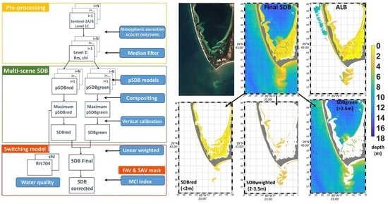
2.5. Satellite-Derived Bathymetry Model

In this study, the ratio model of log-transformed bands having different water absorption was applied (Equations (1) and (2)). The model was designed to support routine mapping in clear waters with extremely limited calibration data [31]. The model uses the Remote Sensing Reflectance (Rrs, units of sr−1) of the blue (490 nm), green (560 nm) and red (664 nm) bands for each satellite image corrected for atmospheric effects (Equations (1) and (2)), and the log-transform addresses the exponential decrease in light with depth [31]. In this case, we used the ratio of blue ( λ i ) to either green or red ( λ j ) bands to produce the SDB (hereinafter called SDBgreen and SDBred, respectively). SDBgreen performs better in deep areas, and SDBred performs better in shallow water [22,23,24,44]:
SDB = m 1 pSDB m 0
where,
pSDB = ln ( n   π Rrs ( λ i ) ) ln ( n   π Rrs ( λ j ) )
pSDB is the relative or “pseudo” depth from satellite (dimensionless), SDB is the satellite-derived depth (meters), Rrs is the Remote Sensing Reflectance, m1 and m0 are tunable constants to linearly transform the model results to actual depth, π has units of sr, and n=1000 is a fixed constant to assure that both logarithms will be positive under any condition and that a residual non-linearity in the ratio is removed from depths that are retrievable from satellite [31].

2.6. Multi-Scene Approach

Thanks to the 5-day revisit of the Sentinel-2 twin satellites, the mission can offer imagery that would identify transient turbidity features that produce false shoals. Accordingly, in this study, we used a multi-scene approach (see Figure 2). The pSDBgreen and pSDBred were determined, per Equation (2), for all available scenes (Table 1). It was reasonable to assume that the contribution from the temporal variability in water-column turbidity to SDB models was greater than the temporal variability of the seafloor [46]. As turbidity produces a false shoaling of depth, all scenes were compared to identify the maximum pSDB at each pixel from all the scenes, and two resultant composite images were created: one of the maximum pSDBred, and one of the maximum pSDBgreen, with assumption being maximum pSDB values would most likely be without any shoal effect. Composite images of Rrs704 and chlorophyll from the OC3 algorithm were also returned, where the turbidity value at each pixel came from the same scene as the depth for that pixel. Both Rrs704 and chl were surrogates for addressing the false shallowing, not intended to describe actual turbidity or chl concentration.

2.7. Vertical Referencing with Chart Soundings

After generating the final pSDBred and pSDBgreen maps, the parameters m1 and m0 (Equation (1)) were tuned by linear regression with about ten control points from charts in each of the study regions and for pSDBred and pSDBgreen separately. Depth measurements (also known, as soundings) from NOAA charts [47] were used to select the control points over Cape Lookout (11545) and Joseph Bay (11389). Using chart points keeps the calibration independent of the lidar used for validation, and corresponds to methods that would be utilized in typical application [31]. The points were chosen as areas of uniform depth that were less likely to have changed over time (regions away from inlets and sand waves). The selected calibration points (pixels) for each of the four composite images were found to originate in different input scenes (3 and 4 different scenes respectively for SDBred and SDBgreen for St- Joseph Bay, and 5 for both Cape Lookout composites). The vertical calibration inherently corrects for the reference data by shifting the depths to the tidal datum, which in the case of USA is the MLLW, through the tuning of the coefficient m0. Sea level depends on satellite observation time; in this case, both regions are microtidal environments. For this approach, our hypothesis was that the influence of the tide for a pSDB relative to each scene is small compared to the influence of the false shallowing generated by turbidity from multiple satellite images. The validation of this hypothesis and the improvement of accuracy by compensating for tide effects in meso and macrotidal regimes are subjects for future study.
In addition, to test the robustness of the multi-scene approach and the final SDB result in terms of a common calibration for remote unsurveyed locations, we interchanged the coefficients for pSDBred and pSDBgreen between the two regions, thus using the coefficients of Cape Lookout in St. Joseph Bay, and vice versa.

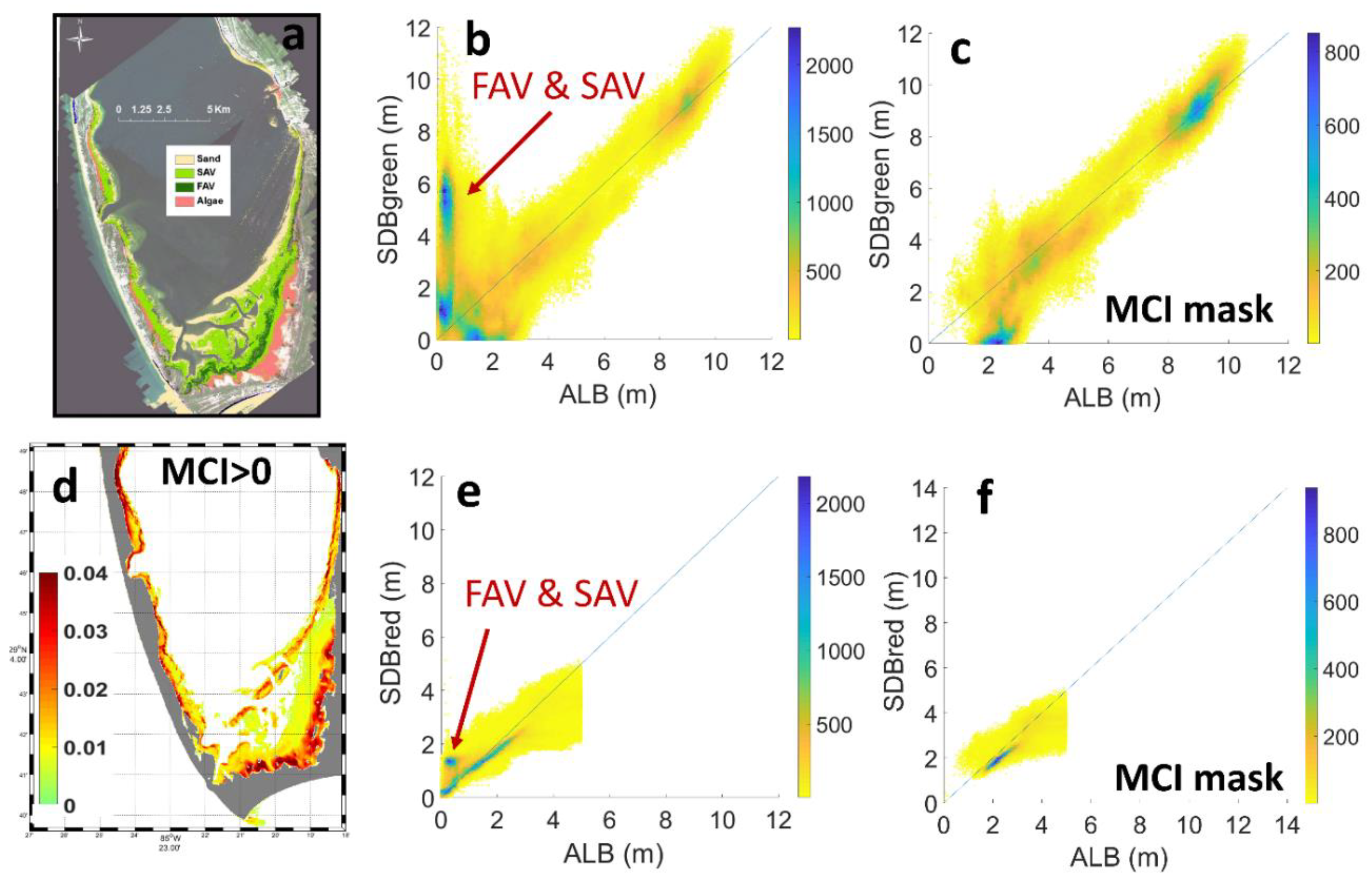
2.8. Switching Model

The final step for a corrected bathymetry mapping (SDB) corresponded to a switching model implementation between SDBred and SDBgreen due to the sensitivity of each model: while SDBred performs better over shallow regions [48], SDBgreen performs better over deeper regions [21,31,44,49]. Moreover, SDBgreen frequently yields severe overestimation in shallow regions [22,44,50], especially with dense seagrass, highly undesirable for navigational purposes. The switch between models used the conditions detailed below:
SDBred < 2 m, SDB=SDBred
SDBred > 2 m and SDBgreen > 3.5 m, SDB=SDBgreen
SDBred >= 2 m and SDBgreen <= 3.5 m, SDB=SDBweighted
SDBweighted was determined by a simple linear weighting calculation to account for a smooth transition (Equation (3)):
S D B = α S D B r e d +   β S D B g r e e n
where the depth weighting (for 3.5 m and 2 m) is determined by:
α = 3.5 S D B r e d 3.5 2   and   β = 1   α  
The final SDB map was generated in each region then compared to the lidar surveys for validation. Assessment of the discrepancy between SDB and lidar used the mean difference as the bias metric, the Median Absolute Error (MedAE) providing the typical total error, and the interquartile range (IQR) as a measure of statistical dispersion. These are robust metrics that do not require an assumption of a Gaussian error distribution.

2.9. Submerged and Floating Aquatic Vegetation Masking
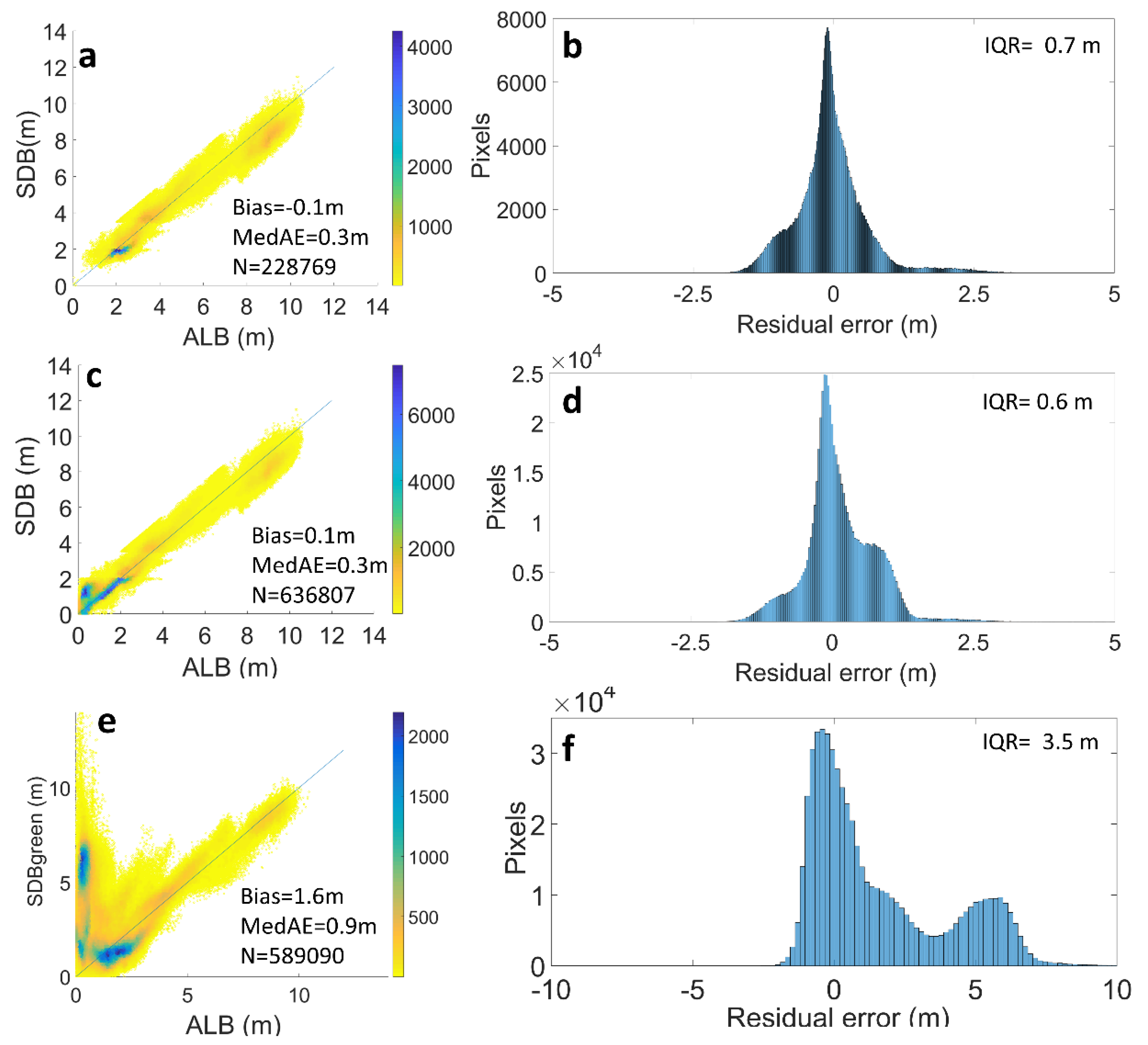
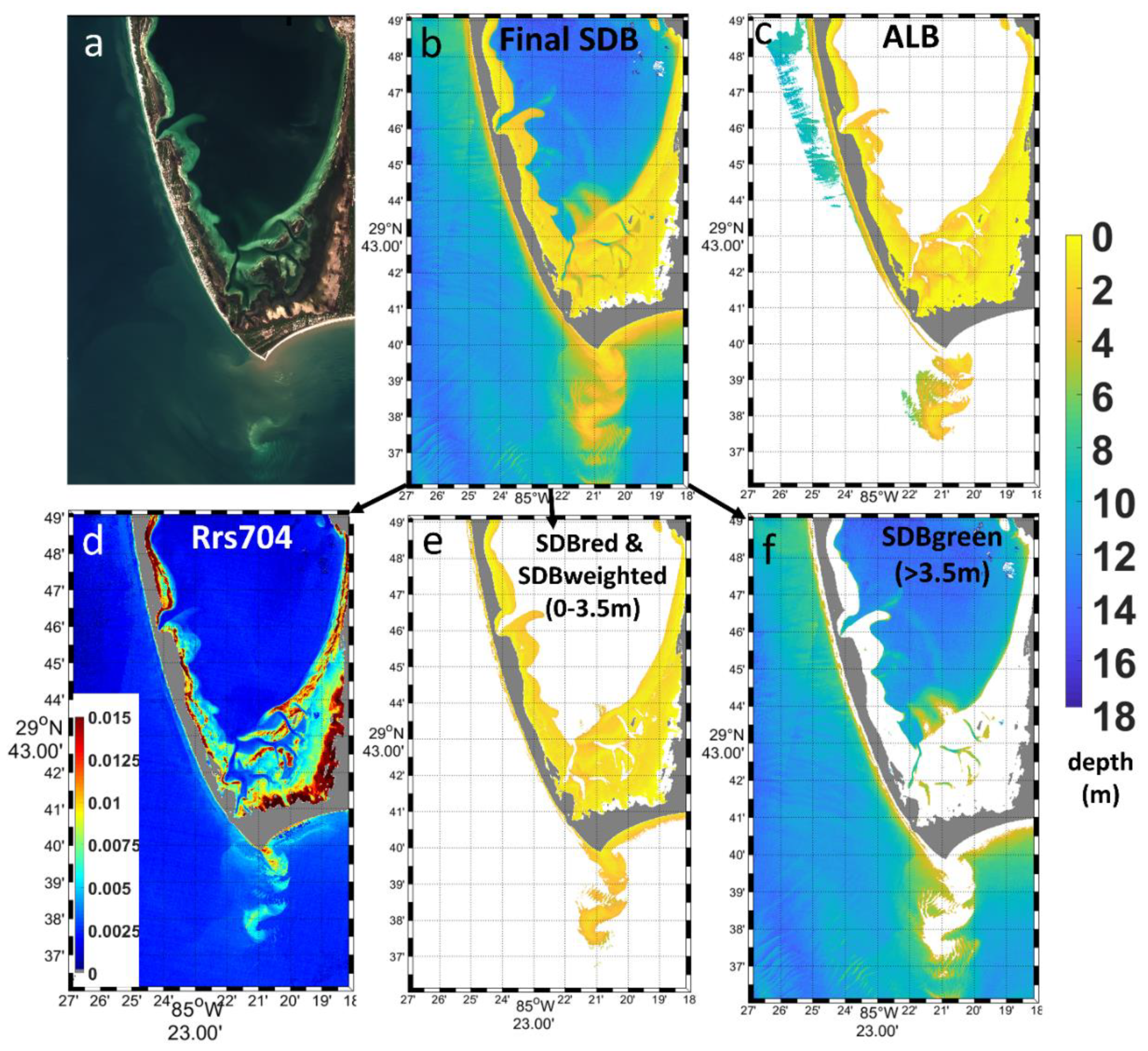
An additional step was carried out in St. Joseph Bay due to the existence of floating aquatic vegetation (FAV) and shallowed submerged aquatic vegetation (SAV). The complex coastal waters of Saint Joseph Bay are characterized by several benthic types, including high density submerged and floating aquatic vegetation at depths shallower than 2 m [51]. In order to correct this issue, we established a masking strategy for the FAV and SAV area. The MCI (Maximum Chlorophyll Index) first designed for the MEdium Resolution Imaging Spectrometer (MERIS), measuring the radiance peak at the red-edge band (709 nm) in water leaving radiance, indicates the presence of a high surface concentration of chlorophyll against a scattering background [52]. This index was formed with three MERIS narrow channels centered near 681, 709 and 754 nm used to define a linear baseline. The MCI has been used to map floating vegetation or benthic [53,54]. In this study, given that Sentinel-2 has three bands (665, 704, and 740 nm) similar to the MERIS bands used for MCI, we utilized Equation (4).
MCI = R r s 704 R r s 665 + ( R r s 665 R r s 740 ) ( R r s 704 R r s 665 ) ( R r s 740 R r s 665 )
FAV and SAV areas were established for the pixels with positive values of MCI (MCI>0). This MCI mask was applied to the final SDB map after the multi-scene approach and switching model in St. Joseph Bay in order to remove possible overestimation for shallow depths where vegetation was present. Therefore, the MCI was not used to map seagrass, but to locate and remove an error source with SDB.

3. Results

3.1. Cape Lookout in North Carolina

Prior to implementing the multi-temporal approach with Sentinel-2A/B images in Cape Lookout (Figure 1b), we estimated bathymetry for several single scenes in order to evaluate the impact of varying turbidity. Figure 3 illustrates two different examples of SDBgreen model for Sentinel-2A on 23 January and 30 October 2017. The heterogeneous impact of water quality on satellite bathymetry is evident in the comparison between Airborne Lidar Bathymetry (hereinafter ALB) and satellite data (Figure 3a,b) and the residual errors (Figure 3c,d). The scatterplots reveal large spread and errors, particularly on 30 October, where an acute underestimation or false shoaling (Figure 3g) and large Median Absolute Error (MedAE=2.95 m) resulted from the higher turbidity levels that are shown in the Remote Sensing Reflectance at 704 nm (Rrs704), a proxy for turbidity (Figure 3h). These outcomes demonstrated the impact of variable water quality conditions on the accuracy of the predicted SDB. Although the 23 January scene had lower turbidity overall—and might be selected as the optimal scene for analysis—there are still areas of elevated turbidity evident offshore (see the lower right of 3e and 3f). Over complex turbid environments such as Cape Lookout [32,34], using only a single scene for SDB has definite limitations.
The compositing selected the pixels of the multiple scenes that were slightly affected by turbidity. Compositing multiple scenes to identify the pixels in order to correct for water turbidity substantially improved the accuracy, as can be observed in Figure 4 and Figure 5. The assumption of the approach is based on the submarine terrain remaining slightly unchanged during the study period (1 year) to accumulate a time series of scenes to use in the compositing, while turbidity (and noise: waves, cloud shadows, ships, and bubbles) affect the accuracy of bathymetric inversion. Using the multi-scene pixel compositing approach with the sixteen images (Table 1), and then applying the switching model between SDBred and SDBgreen, gave better performance from shallow to deeper regions. The composite solution scheme efficiently described the nearshore depth with minimum scatter and MedAE = 0.41 m over the range of ALB data (up to 12.5 m) compared to the individual scenes (Figure 4a,b for composite, and Figure 4c,d for best single scene).
In addition, the switching strategy reduced error over using only SDBred (Figure 6a,c) or SDBgreen (Figure 6b,d). Recently, the switching algorithm has been suggested to be an opportune method for mapping regions from very shallow to deeper waters [22,44]. The quality of the combined models is shown in the histogram of the residual errors, which has a symmetric and narrow distribution (Figure 4b). The vertical calibration results are presented in Figure 7. Compared to the current standard approaches focused on the selection of the optimal scenes; in this case, the clearest image was acquired on 27 November 2017, compositing reduced the mean error by 50% and the IQR from 1.6 m to 0.9 m (Figure 4a,b vs. Figure 4c,d).
The method was evaluated by taking into account the selection of images, confirming that pixels from multiple scenes with high turbidity conditions (Rrs704) and chlorophyll (chl) were minimally incorporated into the model (<1%). Table 1 detailed the percentage of each scene incorporated into the final model. Turbidity (defined as either Rrs704 or chl) produces a false shoaling because the relative or “pseudo” depth pSDB (before the vertical calibration) decreases as turbidity increases (see an example for Cape Lookout in Figure 8). There is a relationship between the increase in the two water quality parameters and the decrease in relative depths for both models, pSDBred and pSDBgreen, thus confirming that intense false shoaling patterns were associated with highly turbid water. Similar results have been found in other sites along the Florida coastal waters using imagery from Sentinel-2A and Sentinel-3A [22]. Figure 5d represents the turbidity proxy (Rrs704) associated with the final SDB map, providing an indication of areas where residual turbidity may exhibit potential residual biases.
The method also exhibited some advantages over the in-situ data. The lidar survey was limited by water clarity as well, and some water areas nearshore were not retrieved (Figure 5c). In contrast, by using multiple dates of imagery, features could be identified by the composited satellite data, along the entire coastal fringe and within the inner banks (SDB on Figure 5b compared to ALB on Figure 5c). We also examined the switching model used in this study, so the final SDB map (Figure 5b) was split into the SDBred and SDBweighted (0-3.5 m, Figure 5e), and the SDBgreen (>3.5 m, Figure 5f). SDBred and SDBweighted mapped the shallow regions within the banks and barrier islands, while the SDBgreen mapped the offshore and the deep channels in the banks. In offshore areas where the bottom was not visible, the attributed depth was removed with a cut-off depth of 17 m. These results were support by visual comparison with the RGB composite (Figure 5a) and standard chart soundings collected by the National Oceanic and Atmospheric Administration [47], given that there was not high-resolution information available for validation of those deeper water areas.

3.2. Saint Joseph Bay in Florida

Previous studies have characterized the Saint Joseph Bay and the adjacent area as a moderately turbid region under influence of the Apalachicola Bay turbid waters [33,35]. The region also has areas of dense shallow aquatic vegetation [51], so a single scene was used to evaluate model performance over these areas. A preliminary inspection of a clear image acquired on 14 February 2017 for SDBred (Figure 9e) and SDBgreen (Figure 9b) demonstrated the impact of FAV and SAV, showing overestimation at depths <1 m over the dense marine vegetation areas for both models. The overestimate was about 1 m for SDB red and severe at up to 6 m for SDBgreen. Inspection of other individual scenes also presented overall positive bias for depths <1 m, owing to an apparent higher absorption of the green band (560 nm) for SDBgreen, whereas lower relative absorption occurred over vegetation in the red band (664 nm) for SDBred. This was apparently due to the dark signatures of the floating aquatic vegetation (FAV) and submerged aquatic vegetation (SAV) that may cause the overestimation of depth by this model or other SDB approaches.
In order to correct the overestimation issue, a masking procedure to locate and remove an error source based on a common algae index—the Maximum Chlorophyll Index MCI [53,54]—was developed. In [54], it is shown that slightly submerged vegetation will cause an MCI (false positive against phytoplankton). This approach allowed us to use the satellite without requiring any additional in-situ information. Pixels with positive MCI values (MCI>0) were identified as vegetation (Figure 5d) and then masked out. The scatterplots of ALB against SDBred and SDBgreen after masking vegetation (Figure 9c,f, respectively) show that the overestimation was eliminated, thus MCI can be applied to remove the overestimation. Very shallow SDBred pixels with good accuracy (lying on the 1:1 line) were also eliminated, because MCI does register on bright sand in very shallow water (owing to the signal from Rrs704 in <1 m). As a conservative solution, the FAV and SAV masking procedure would be appropriate owing to the severe consequences of overestimating very shallow bathymetry, as identified by the Chart Standards Groups (CSG) at NOAA’s Office of Coast Survey/Marine Chart Division.
The same multi-scene approach and switching model as used for Cape Lookout was carried out in this region, although only seven cloud-free images were available during the study period (Table 1). In this case, we tested the additional MCI masking to remove issues associated with FAV and SAV. The validation against lidar data confirmed the high accuracy obtained for the entire strategy with (Figure 10a) or without (Figure 10c) MCI masking. There was low scatter (MedAE=0.3 m) for depths up to 11 m (limit of ALB data set). The vertical calibration results are presented in Figure 7. Even without MCI correction, the switching model alone substantially reduced intense overestimation of SDBgreen for depths <1 m (Figure 10c). The importance of the switching strategy is evident in the validation of the final multi-scene SDBred and SDBgreen, where an acute overestimation occurred at depths <1 m for SDBgreen, similar to Cape Lookout (Figure 6a–d). In terms of error assessment, the distribution of the residuals indicated minimum discrepancies were achieved (Figure 10b,d). Furthermore, the compositing algorithm produced accurate SDB results compared to the single “optimal scene” approach (picking the scene with the lowest overall turbidity) combined with the most widely used model in the literature, SDBgreen (Figure 10e,f). The composite map of the proxy for turbidity (Rrs704) associated to the final SDB model shows minimum turbid conditions throughout (Figure 11d).
The geographic distribution of features in the SDB (Figure 11b) corresponded to those identifiable in the lidar survey (Figure 11c), although much more spatial information is available in the SDB product. Similar to Cape Lookout region, the method offered a complete map of the St. Joseph coastal area compared to the restricted map provided by lidar surveys. In this case, we did not apply the MCI masking to add data over the vegetated area (depths <1 m), thereby allowing maximum coverage of the final SDB product. Shallow areas and shoals < 3.5 m were accurately described with SDBred and SDBweighted (Figure 11e) whereas depths >3.5 m were mapped with SDBgreen (Figure 11f).

4. Discussion

In the present investigation, we successfully applied both Sentinel-2A and 2B satellites to estimate water depth in two areas with complex bathymetry and water clarity, Cape Lookout, North Carolina, and Saint Joseph Bay, Florida. The multi-scene compositing approach addressed limitations inherent in conventional methods and reduced the impact of turbidity, performing better than the standard “pick the best scene” method that relies on a single image (Figure 3 and Figure 4c vs. Figure 4a in Cape Lookout; and Figure 10e vs. Figure 10a,c in Saint Joseph Bay). The final corrected SDB produced robust depths up to the limit of the lidar surveys, with typical errors ≤0.4 m. These excellent results from Sentinel-2 compared favorably with those produced in relatively low turbidity water in south Florida [22,44], and in regions with transparent waters [10,18,20,30]. Whereas some researchers suggested there is still work to be performed regarding the identification of the optimal period throughout the year where bathymetric errors are minimized [18,29], others asked for novel strategies to allow seabed mapping without the laborious analysis per image and the visual inspection of the “clearest scene” [19]. Recent studies have already indicated the potential of multi-scene approaches in order to select the optimal scene or eliminate noise over clear waters [16,17,19,20]. However, our temporal compositing strategy successfully reduced the turbidity impact without requirement of visual inspection, thereby enhancing SDB performance in an easy way. The high temporal resolution and interchangeability of the Sentinel-2 twin mission may rapidly overcome SDB anomalies introduced by highly heterogeneous water transparency regimes [22].
The multi-scene strategy applied here did not require any screening or manual adjustment of the imagery prior to compositing. It automatically picked the pixels least impacted by turbidity (e.g., Figure 8) from the set of scenes provided (Table 1), substantially simplifying the effort compared with other studies where the selection of optimal images with variation in the water quality conditions were essential in the extraction of SDB [20,22,29,55]. Manual selection of the optimal scene is not only highly subjective, but requires considerable time and effort, and may still include regions having patches of turbidity. The consistency in the pSDB products, which were not yet calibrated to true depth, indicated that ACOLITE produced an effective and robust atmospheric correction across scenes (Figure 8), as previously demonstrated [22,44]. Inconsistencies or errors in ACOLITE (or any other atmospheric correction) would force manual intervention and make compositing impractical [10].
We chose chart values for the calibration to depth in order to demonstrate the benefit of the method for remote areas under likely applied conditions, rather than under the optimal (and extremely unlikely) condition of a contemporaneous lidar survey. Using limited chart soundings would have only introduced some of the error, most likely as bias in the depth. Some depth errors may also be due to the differences in resolution, i.e., 10 m from the satellite, and the 1 m spot size for lidar—a consideration in areas with steep gradients, such as channel edges. Using a median filter on the SDB reduced other artifacts that typically lead to random noise [49]. One potential error factor that needs to be considered in the future is tide range. The tide range in these areas is relatively small (< 1 m). The influence of tide on the accuracy of this approach for areas with tidal ranges greater than 1 m requires further investigation. For meso-tidal areas, one option would be to constrain the input images to a common range of water level, such as 1 m maximum difference in water level. Macro-tidal areas are likely to be too turbid for optical SDB.
An interesting consideration is that the calibration to depth for this method may be dependent on water clarity rather than on geography. Applying the coefficients for composited pSDBred and pSDBgreen of Cape Lookout to St. Joseph Bay (Figure 7), and vice versa, generated precise SDB for both areas with errors ≤0.65 m (see results in Figure 12). This comparison suggests that an existing calibration after the multi-scene approach may be applicable to other remote and unsurveyed areas, assuming the compositing can retrieve the same turbidity. These results suggest the potential suitability of SDB estimates for charting applications using the IHO S-57 standard [56], which defines CATZOC levels containing depth accuracy specifications for depth ranges up to 30 m in order to allow for their incorporation into nautical products.
The use of the SDBred for shallow water retrieval addressed the worst of the overestimation issues with the SDBgreen in both study regions. The use of different bands to treat overestimation in shallow water (or underestimation by SDBred in deep water) has been pointed out recently by some researchers [19,30,57]. Switching to SDBred has been previously used to provide better discrimination of depths in very shallow water over bright targets like carbonate sand [48], and other studies have applied each model over different depth ranges [22,44]. Here, we established an automated switching method between SDBred and SDBgreen that performed accurately over the two study sites. In addition, SDBgreen overestimated on dense seagrass in extremely shallow water using either the single scene (Figure 9b, Figure 10e) or the multi-scene approach (dense seagrass has a very low albedo, so in deeper water there is often no detectable signal to be retrieved from satellite). By switching to the SDBred, the combined product reduced most of the impact of shallow seagrass on SDBgreen (as seen in Figure 9b against Figure 9e or Figure 10e against Figure 10c). If more rigorous masking is required, the MCI can identify the presence of dense seagrass in extremely shallow water (<1–2 m, Figure 10a), without the need for external data sets on bottom type. Combined with calibration using only a few points (Figure 7), the approach detailed here offers an effective means of assessing bathymetry in regions lacking any data.
While the accuracy of SDB cannot match ALB, the spatial coverage of satellite imagery shown here surpasses ALB (Figure 5c and Figure 11c vs. Figure 5b and Figure 11b). This capability represents one of the great benefits of satellite monitoring; whereas in-situ surveys (lidar, sonar) are expensive and extremely limited due to technical and deployment cost, SDB can give us a broad picture of the entire study site with wide swaths, low-cost repeated coverage, and easy access to remote locations [8]. Lidar data is also constrained by availability and water quality, so information can be lost. We characterized post Hurricane Matthew bathymetry in Cape Lookout, extending the limited amount of lidar data to a much larger and more complete area.
Sentinel-2 may provide a way to use other satellites more effectively. Accordingly, Sentinel-2 might offer a low turbidity reference data set that can be used to inform mapping conducted with the various commercial very high-resolution sensors such as the World-View fleet [14,26,58] or the novel CubeSats from Planet [19,29]. On the other scale, Landsat has a four-decade history using Thematic Mapper, and has been shown to be useful for some SDB in clear water [10,21,59,60], even with 30 m pixels. Comparisons of Sentinel-2 with Landsat-8 may ultimately lead to results that could expand the utility of the entire Landsat data record for change detection.
In this study, interpretation of error assessment and uncertainty can be achieved by means of the water quality composites of turbidity (Rrs704) associated with the final SDB maps (Figure 5d and Figure 11d). These products may indicate areas that still have residual bias. They can also provide areas where the water is chronically optically deep due to turbidity, which can lead to better allocation of resources. Previous research has detailed the impact of water quality parameters on SDB results using the ratio model over several regions in Florida [22]. Recent studies using the ratio model showed that bottom reflectance has little influence on the accuracy of SDB estimates, while chlorophyll concentration has a strong influence [22,61]. This problem would also be resolved with the compositing method.
In accordance with our findings, the portability and reliability application of the proposed approach using minimum in-situ measurements is a distinct advantage in effectiveness and may especially benefit developing countries. In addition, using the semi-automated solution and a computer cloud-based system may allow exploitation of the Sentinel-2 data for regional to global scale coastal SDB [16]. The average time required for processing a Sentinel-2 image for bathymetry estimation is ~ 1 hour. For further avenues of research with Sentinel-2, we intend to upscale the study results to more environments with different water and atmospheric conditions in order to evaluate repeatability as well as implement the multi-temporal approach in cloud-based computing platforms such as the ESA Coastal Thematic Exploitation Platform—Coastal-TEP [62]. The promising transferability of this temporal technique exploiting the open and free archive of the Sentinel-2 mission will allow advancement of SDB applications and optimized scientific coastal mapping worldwide, especially in data-poor regions [63].

5. Concluding Remarks

This paper presents a framework to obtain SDB while potentially automated the image processing. Precise SDB was derived over moderately turbid environments by using the high revisit time (5-day) of the Sentinel-2A/B twin mission from the Copernicus programme. The proposed methodology incorporates a robust atmospheric correction with ACOLITE, a multi-scene compositing method to reduce the impact of turbidity, and a switching model to improve mapping in shallow water. Two study sites in United States were explored due to their varying water transparency conditions. The method establishes a plausible high-quality strategy for SDB with sufficient sensitivity to support interannual and pre-post hazards (e.g., hurricanes or tropical storms), which may benefit change detection analysis from multiple images to discriminate variability. The open data policy and long-term mission commitment of Sentinel-2 opens future promising time series evaluation over years and even decades that can be an important tool to provide crucial missing information on the bathymetry distribution, especially in data-poor or remote areas with large gaps in a retrospective, rapid and non-intrusive manner. It would enable immediate commencement of coastal mapping using archived and/or forthcoming imagery from the Copernicus programme at regional to global spatial scales, and any other source from which repeated scenes may be collected over the world’s coastal systems. There is a requirement to promote the development of technology that provides low-cost solutions with enhanced data quality to address the needs of a wide range of user groups. The semi-automated framework demonstrated here may address that need, and help mitigate the long-standing gap of depth information for the majority of coastal regions on Earth. Such a capability can aid scientists, managers, and policymakers around the globe in assessing vulnerabilities to ecosystems, infrastructure, navigation and many other coastal concerns.

Author Contributions

I.C. and R.P.S. conceived and designed the research. I.C. collected the remote sensing data, processed the data, conducted the analysis, and prepared the figures. R.P.S. supervised the research. I.C. led the writing of the manuscript with contribution from R.P.S. All authors have read and agreed to the published version of the manuscript.

Funding

Isabel Caballero was funded by the National Oceanic and Atmospheric Administration and the National Academy of Science, Engineering and Medicine under the NRC postdoctoral Research Associateship Program (RAP) 2017-2019 with support from the NOAA-Korea Ministry of Oceans and Fisheries Joint Project Agreement. This research was also supported by the Sen2Coast Project (RTI2018-098784-J-I00) funded by the Ministry of Science, Innovation and Universities (MCIU), the State Research Agency (AEI) and the European Regional Development Fund (ERDF).

Acknowledgments

The authors thank the European Space Agency, the European Commission and the Copernicus programme for distributing Sentinel-2 imagery. Thanks to the National Oceanic and Atmospheric Administration and the National Geodetic Survey for providing the valuable high-resolution lidar data and the nautical charts used for this study. Thanks to Quinten Vanhellemont for his assistance in using ACOLITE processor. The authors acknowledge the three anonymous reviewers, whose comments helped to greatly improve an earlier version of this manuscript.

Conflicts of Interest

The authors declare no conflict of interest.

References

  1. United Nations. Transforming Our World: The 2030 Agenda for Sustainable Development. 2015. Available online: https://sustainabledevelopment.un.org/post2015/transformingourworld/publication (accessed on 10 June 2019).
  2. Charles, E.; Douvere, F. Marine Spatial Planning: A Step-by-Step Approach toward Ecosystem-Based Management. Intergovernmental Oceanographic Commission and Man and the Biosphere Programme. IOC Manual and Guides; ICAM Dossier No. 6; UNESCO: Paris, France, 2009; p. 99. [Google Scholar]
  3. International Hydrographic Organization. International Hydrographic Review. 2017. Available online: https://www.iho.int/mtg_docs/IHReview/2017/IHR_May2017.pdf (accessed on 15 October 2019).
  4. International Hydrographic Organization. International Hydrographic Review. 2017. Available online: https://www.iho.int/mtg_docs/IHReview/2017/IHR_November2017.pdf (accessed on 15 October 2019).
  5. International Hydrographic Organization. International Hydrographic Publication C-55 Status of Hydrographic Surveying and Charting Worldwide. 2018. Available online: http://iho.int/mtg_docs/misc_docs/basic_docs/IHO_Work_Programme_for_2019_final.pdf (accessed on 15 October 2019).
  6. Carron, M.J.; Vogt, P.R.; Jung, W.Y. A proposed international long-term project to systematically map the world’s ocean floors from beach to trench: GOMaP (Global Ocean Mapping Program). Int. Hydrogr. Rev. 2001, 2. [Google Scholar]
  7. Marks, K.M. International Hydrographic Organization, Intergovernmental Oceanographic Commission, The IHO-IOC GEBCO Cook Book; IHO Publication B-11, IOC Manuals and Guides 63; IOC: Monaco, France, 2019; 493p. [Google Scholar]
  8. Gao, J. Bathymetric mapping by means of remote sensing: Methods, accuracy and limitations. Prog. Phys. Geogr. 2009, 33, 103–116. [Google Scholar] [CrossRef]
  9. Dekker, A.G.; Phinn, S.R.; Anstee, J.; Bissett, P.; Brando, V.E.; Casey, B.; Fearns, P.; Hedley, J.; Klonowski, W.; Lee, Z.P.; et al. Intercomparison of shallow water bathymetry, hydro-optics, and benthos mapping techniques in Australian and Caribbean coastal environments. Limnol. Oceanogr. Methods 2011, 9, 396–425. [Google Scholar] [CrossRef] [Green Version]
  10. Hedley, J.D.; Roelfsema, C.; Brando, V.; Giardino, C.; Kutser, T.; Phinn, S.; Mumby, P.; Barrilero, O.; Laporte, J.; Koetzh, B. Coral reef applications of Sentinel-2: Coverage, characteristics, bathymetry and benthic mapping with comparison to Landsat 8. Remote Sens. Environ. 2018, 216, 598–614. [Google Scholar] [CrossRef]
  11. Tripathi, N.K.; Rao, A.M. Bathymetric mapping in Kakinada Bay, India, using IRS-1D LISS-III data. Int. J. Remote Sens. 2002, 23, 1013–1025. [Google Scholar] [CrossRef]
  12. Philpot, W.D.; Davis, C.O.; Bissett, W.P.; Mobley, C.D.; Kohler, D.C.D.; Lee, Z.; Bowles, J.; Steward, R.G.; Agrawal, Y.; Trowbridge, J.; et al. Bottom Characterization from Hyperspectral Image Data. Oceanography 2004, 17, 76–85. [Google Scholar] [CrossRef]
  13. Minghelli-Roman, A.; Dupouy, C. Influence of water column chlorophyll concentration on bathymetric estimations in the lagoon of New Caledonia, using several MERIS images. IEEE J. Sel. Top. Appl. Earth Obs. Remote Sens. 2013, 6, 739–745. [Google Scholar] [CrossRef] [Green Version]
  14. Hamylton, S.M.; Hedley, J.D.; Beaman, R.J. Derivation of high-resolution bathymetry from multispectral satellite imagery: A comparison of empirical and optimization methods through geographical error analysis. Remote Sens. 2015, 7, 16257–16273. [Google Scholar] [CrossRef] [Green Version]
  15. Khondoker, M.S.I.; Siddiquee, M.Z.H.; Islam, M. The Challenges of River Bathymetry Survey Using Space Borne Remote Sensing in Bangladesh. Atmos. Ocean. Sci. 2016, 1, 7–13. [Google Scholar]
  16. Traganos, D.; Poursanidis, D.; Aggarwal, B.; Chrysoulakis, N.; Reinartz, P. Estimating satellite-derived bathymetry (SDB) with the google earth engine and sentinel-2. Remote Sens. 2018, 10, 859. [Google Scholar] [CrossRef] [Green Version]
  17. Chu, S.; Cheng, L.; Ruan, X.; Zhuang, Q.; Zhou, X.; Li, M.; Shi, Y. Technical Framework for Shallow-Water Bathymetry With High Reliability and No Missing Data Based on Time-Series Sentinel-2 Images. IEEE Trans. Geosci. Remote Sens. 2019, 57, 1–19. [Google Scholar] [CrossRef]
  18. Evagorou, E.G.; Mettas, C.; Agapiou, A.; Themistocleous, K.; Hadjimitsis, D.G. Bathymetric maps from multi-temporal analysis of Sentinel-2 data: The case study of Limassol, Cyprus. Adv. Geosci. 2019, 45, 397–407. [Google Scholar] [CrossRef] [Green Version]
  19. Poursanidis, D.; Traganos, D.; Chrysoulakis, N.; Reinartz, P. Cubesats Allow High Spatiotemporal Estimates of Satellite-Derived Bathymetry. Remote Sens. 2019, 11, 1299. [Google Scholar] [CrossRef] [Green Version]
  20. Sagawa, T.; Yamashita, Y.; Okumura, T.; Yamanokuchi, T. Satellite Derived Bathymetry Using Machine Learning and Multi-Temporal Satellite Images. Remote Sens. 2019, 11, 1155. [Google Scholar] [CrossRef] [Green Version]
  21. Pe’eri, S.; Madore, B.; Nyberg, J.; Snyder, L.; Parrish, C.; Smith, S. Identifying bathymetric differences over Alaska’s North Slope using a satellite-derived bathymetry multi-temporal approach. J. Coast. Res. 2016, 76, 56–63. [Google Scholar] [CrossRef]
  22. Caballero, I.; Stump, P.R.; Meredith, A. Preliminary assessment of turbidity and chlorophyll impact on bathymetry derived from Sentinel-2A and Sentinel-3A satellites in South Florida. Remote Sens. 2019, 11, 645. [Google Scholar] [CrossRef] [Green Version]
  23. Stumpf, R.P.; Feldman, G.C.; Kuring, N.; Franz, B.; Green, E.; Robinson, J. SeaWiFS spies reefs. Reef Encount. 1990, 26, 29–30. [Google Scholar]
  24. National Aeronautics and Space Administration. Remote Sensing of Coral Reefs: SeaWiFS Bathymetry and Data Archive Proof-of-Concept. 2003. Available online: https://oceancolor.gsfc.nasa.gov/cgi/reefs.pl (accessed on 15 September 2019).
  25. Minghelli-Roman, A.; Goreac, A.; Mathieu, S.; Spigai, M.; Gouton, P. Comparison of bathymetric estimation using different satellite images in coastal sea waters. Int. J. Remote Sens. 2009, 30, 5737–5750. [Google Scholar] [CrossRef]
  26. Kanno, A.; Tanaka, Y.; Shinohara, R.; Kurosawa, A.; Sekine, M. Which spectral bands of Worldview-2 are useful in remote sensing of water depth? A case study in coral reefs. Mar. Geod. 2014, 37, 283–292. [Google Scholar] [CrossRef]
  27. European Commission. Copernicus for Coastal Zone Monitoring and Management Workshop; Technical Report; Copernicus Support Office, 2017; Available online: https://land.copernicus.eu/user-corner/technical-library/report-of-the-coastal-zone-monitoring-and-management-workshop (accessed on 1 October 2019).
  28. Canadian Hydrographic Service. First international Hydrographic Remote Sensing (HRS) workshop, workshop report. In Proceedings of the First International Hydrographic Remote Sensing (HRS) Workshop, Ottawa, ON, Canada, 18–20 September 2018. [Google Scholar]
  29. Li, J.; Schill, S.R.; Knapp, D.E.; Asner, G.P. Object-Based Mapping of Coral Reef Habitats Using Planet Dove Satellites. Remote Sens. 2019, 11, 1445. [Google Scholar] [CrossRef] [Green Version]
  30. Poursanidis, D.; Traganos, D.; Reinartz, P.; Chrysoulakis, N. On the use of Sentinel-2 for coastal habitat mapping and satellite-derived bathymetry estimation using downscaled coastal aerosol band. Int. J. Appl. Earth Obs. Geoinf. 2019, 80, 58–70. [Google Scholar] [CrossRef]
  31. Stumpf, R.P.; Holderied, K.; Sinclair, M. Determination of water depth with high-resolution satellite imagery over variable bottom types. Limnol. Oceanogr. 2003, 48 Pt 2, 547–556. [Google Scholar] [CrossRef]
  32. Wells, J.T. Accumulation of fine-grained sediments in a periodically energetic clastic environment, Cape Lookout Bight, North Carolina. J. Sediment. Res. 1988, 58, 596–606. [Google Scholar]
  33. Berndt, M.P.; Franklin, M.A. Water-Quality and Discharge Data for St. Joseph Bay, Florida, 1997–1998; Department of the Interior: Washington, DC, USA, 1999; Available online: https://apps.dtic.mil/dtic/tr/fulltext/u2/a442268.pdf (accessed on 1 October 2019).
  34. Mienis, F.; Duineveld, G.C.A.; Davies, A.J.; Lavaleye, M.M.S.; Ross, S.W.; Seim, H.; Brooke, S. Cold-water coral growth under extreme environmental conditions, the Cape Lookout area, NW Atlantic. Biogeosciences 2014, 11, 2543–2560. [Google Scholar] [CrossRef] [Green Version]
  35. Joshi, I.D.; D’Sa, E.J.; Osburn, C.L.; Bianchi, T.S. Turbidity in Apalachicola bay, Florida from Landsat 5 TM and field data: Seasonal patterns and response to extreme events. Remote Sens. 2017, 9, 367. [Google Scholar] [CrossRef] [Green Version]
  36. European Space Agency. Sentinel-2 User Handbook; ESA Standard Document; ESA: Paris, France, 2015; Available online: https://sentinel.esa.int/documents/247904/685211/Sentinel-2_User_Handbook (accessed on 20 June 2019).
  37. Sentinel’s Scientific Data Hub. Available online: https://scihub.copernicus.eu/ (accessed on 15 May 2019).
  38. European Space Agency. Sentinel-2 MSI Technical Guide. 2017. Available online: https://earth.esa.int/web/sentinel/technical-guides/sentinel-2-msi (accessed on 5 May 2019).
  39. Vanhellemont, Q.; Ruddick, K. Turbid wakes associated with offshore wind turbines observed with Landsat 8. Remote Sens. Environ. 2014, 145, 105–115. [Google Scholar] [CrossRef] [Green Version]
  40. Vanhellemont, Q.; Ruddick, K. Advantages of high quality SWIR bands for ocean colour processing: Examples from Landsat-8. Remote Sens. Environ. 2015, 161, 89–106. [Google Scholar] [CrossRef] [Green Version]
  41. Vanhellemont, Q.; Ruddick, K. Acolite for Sentinel-2: Aquatic Applications of MSI Imagery. In Proceedings of the ESA Living Planet Symposium, Prague, Czech Republic, 9–13 May 2016. [Google Scholar]
  42. Ruddick, K.; Vanhellemont, Q.; Dogliotti, A.; Nechad, B.; Pringle, N.; Van der Zande, D. New Opportunities and Challenges for High Resolution Remote Sensing of Water Colour. In Proceedings of the Ocean Optics XXIII, Victoria, BC, Canada, 7 October 2016. [Google Scholar]
  43. Pahlevan, N.; Sarkar, S.; Franz, B.A.; Balasubramanian, S.V.; He, J. Sentinel-2 MultiSpectral Instrument (MSI) data processing for aquatic science applications: Demonstrations and validations. Remote Sens. Environ. 2017, 201, 47–56. [Google Scholar] [CrossRef]
  44. Caballero, I.; Stumpf, R.P. Retrieval of nearshore bathymetry from Sentinel-2A and 2B satellites in South Florida coastal waters. Estuar. Coast. Shelf Sci. 2019, 226, 106277. [Google Scholar] [CrossRef]
  45. Toming, K.; Kutser, T.; Laas, A.; Sepp, M.; Paavel, B.; Nõges, T. First experiences in mapping lake water quality parameters with Sentinel-2 MSI imagery. Remote Sens. 2016, 8, 640. [Google Scholar] [CrossRef] [Green Version]
  46. Davis, R.A.; Fitzgerald, D.M. Beaches and Coasts; Blackwell Publishing Company: Malden, MA, USA, 2014; p. 419. [Google Scholar]
  47. National Oceanic and Atmospheric Administration. NOAA Nautical Chart Catalog and Locator. 2019. Available online: http://www.charts.noaa.gov/ (accessed on 1 May 2019).
  48. National Oceanic and Atmospheric Administration. Atlas of the Shallow-Water Benthic Habitats of the Northwestern Hawaiian Islands. 2003; p. 160. Available online: https://cdn.coastalscience.noaa.gov/datasets/e98/docs/NWHI_Atlas_sec1.pdf (accessed on 1 May 2019).
  49. Linklater, M.; Hamylton, S.M.; Brooke, B.P.; Nichol, S.L.; Jordan, A.R.; Woodroffe, C.D. Development of a seamless, high-resolution bathymetric model to compare reef morphology around the subtropical island shelves of Lord Howe Island and Balls Pyramid, southwest Pacific Ocean. Geosciences 2018, 8, 11. [Google Scholar] [CrossRef] [Green Version]
  50. Bramante, J.F.; Raju, D.K.; Sin, T.M. Multispectral derivation of bathymetry in Singapore’s shallow, turbid waters. Int. J. Remote Sens. 2013, 34, 2070–2088. [Google Scholar] [CrossRef]
  51. Hill, V.J.; Zimmerman, R.C.; Bissett, W.P.; Dierssen, H.; Kohler, D.D. Evaluating light availability, seagrass biomass, and productivity using hyperspectral airborne remote sensing in Saint Joseph’s Bay, Florida. Estuar. Coasts 2014, 37, 1467–1489. [Google Scholar] [CrossRef]
  52. Gitelson, A. The peak near 700 nm on radiance spectra of algae and water: Relationships of its magnitude and position with chlorophyll concentration. Int. J. Remote Sens. 1992, 13, 3367–3373. [Google Scholar] [CrossRef]
  53. Gower, J.; King, S. Distribution of floating Sargassum in the Gulf of Mexico and the Atlantic Ocean mapped using MERIS. Int. J. Remote Sens. 2011, 32, 1917–1929. [Google Scholar] [CrossRef]
  54. Gower, J.; King, S.; Borstad, G.; Brown, L. Detection of intense plankton blooms using the 709 nm band of the MERIS imaging spectrometer. Int. J. Remote Sens. 2005, 26, 2005–2012. [Google Scholar] [CrossRef]
  55. Casal, G.; Monteys, X.; Hedley, J.; Harris, P.; Cahalane, C.; McCarthy, T. Assessment of empirical algorithms for bathymetry extraction using Sentinel-2 data. Int. J. Remote Sens. 2019, 40, 2855–2879. [Google Scholar] [CrossRef]
  56. International Hydrographic Organization IHO. S-57 Supplement No. 3-Supplementary Information for the Encoding of S-57 Edition 3.1 ENC Data; International Hydrographic Organization: Monaco, France, 2014; Available online: https://www.iho.int/iho_pubs/standard/S-57Ed3.1/S-57_e3.1_Supp3_Jun14_EN.pdf (accessed on 5 September 2019).
  57. Geyman, E.C.; Maloof, A.C. A simple method for extracting water depth from multispectral satellite imagery in regions of variable bottom type. Earth Space Sci. 2019, 6, 527–537. [Google Scholar] [CrossRef]
  58. Eugenio, F.; Marcello, J.; Martin, J. High-resolution maps of bathymetry and benthic habitats in shallow-water environments using multispectral remote sensing imagery. IEEE Trans. Geosci. Remote Sens. 2015, 53, 3539–3549. [Google Scholar] [CrossRef]
  59. Pacheco, A.; Horta, J.; Loureiro, C.; Ferreira, Ó. Retrieval of nearshore bathymetry from Landsat 8 images: A tool for coastal monitoring in shallow waters. Remote Sens. Environ. 2015, 159, 102–116. [Google Scholar] [CrossRef] [Green Version]
  60. Kabiri, K. Accuracy assessment of near-shore bathymetry information retrieved from Landsat-8 imagery. Earth Sci. Inform. 2017, 10, 235–245. [Google Scholar]
  61. Kerr, J.M.; Purkis, S. An algorithm for optically-deriving water depth from multispectral imagery in coral reef landscapes in the absence of ground-truth data. Remote Sens. Environ. 2018, 210, 307–324. [Google Scholar] [CrossRef]
  62. Coastal Thematic Exploitation Platform—Coastal-TEP. Available online: https://www.coastal-tep.eu/geobrowser/ (accessed on 20 November 2019).
  63. Wölfl, A.C.; Snaith, H.; Amirebrahimi, S.; Devey, C.W.; Dorschel, B.; Ferrini, V.; Lamarche, G. Seafloor Mapping–the challenge of a truly global ocean bathymetry. Front. Mar. Sci. 2019, 6, 283. [Google Scholar]
Figure 1. Location of the study regions in the east coast of United States. (a) RGB composite of Saint Joseph Bay in Florida from Sentinel-2A tile T16RFT (February 24, 2017), and (b) RGB composite of Cape Lookout in North Carolina from Sentinel-2B tile T18SUD (September 28, 2017). The rectangles indicate the Region of Interest (ROI) for bathymetric mapping.
Remotesensing 12 00451 g001
Figure 2. A schematic workflow of processing steps implemented for mapping Satellite-Derived Bathymetry with temporal imagery of Sentinel-2A and 2B satellites in Cape Lookout and Saint Joseph Bay: (1) Pre-processing, (2) Multi-scene SDB approach, (3) Switching model, and Submerged aquatic vegetation (SAV) and floating aquatic vegetation (FAV) masking (only in Joseph Bay).
Remotesensing 12 00451 g002
Figure 3. Comparison between lidar (ALB) and Sentinel-2 bathymetry (SDBgreen) for two individual scenes from the Cape Lookout, NC study area. (a) scatter frequency plots for 23 January and (b) 30 October 2017, the color bars indicate pixel frequency at the point; residual errors (SDBgreen—ALB) for (c) 23 January (standard deviation = 2.07 m, percentile 5%/95% = −4.06 m/2.93 m), and (d) 30 October (standard deviation = 3.17 m, percentile 5%/95% = −6.88 m/3.16 m), the bins of the histograms correspond to the number of pixels; maps of SDBgreen for (e) 23 January and (g) 30 October; and maps of the turbidity proxy used in this study, Remote Sensing Reflectance at 704 nm (Rrs704), for (f) 23 January and (h) 30 October. Gray color represents land mask and white color at the left is the limit of Sentinel-2 tile for each date.
Remotesensing 12 00451 g003
Figure 4. Comparison between lidar (ALB) and final SDB in Cape Lookout. (a) Scatter frequency of the final SDB after the multi-scene approach and switching model, the color bars indicate pixel frequency, (b) Associated histogram of residual errors with standard deviation=1.1m and percentile 5%/95%=-2.36m/0.93m, where the total number of pixels is N = 271635, divided in SDBred for depths <2 m with N = 148710 (54.7%), SDBweighted for depths 2-3.5 m with N = 30115 (11.1%), and SDBgreen for depths >3.5 m with N = 92810 (34.2%); (c), scatter frequency of the SDBgreen compared to ALB for the clearest scene acquired on 27 November 2017 (N = 227438), and (f) Associated histogram of residual errors and (d) with standard deviation=1.29m and percentile 5%/95%=-2.3m/1.89m, the bins of the histograms correspond to the number of pixels.
Remotesensing 12 00451 g004
Figure 5. Satellite maps in Cape Lookout region. (a) Sentinel-2 RGB image composite, (b) Final SDB after the multi-scene approach and the switching model, (c) Lidar (ALB) data collected by NOAA, (d) Remote sensing reflectance at 704 nm (Rrs704) associated with the final SDB, segmentation of the final SDB with the switching model: (e) SDBred for depths <2 m and SDBweighted for depths 2–3.5 m, and (f) SDBgreen for depths >3.5 m. Data in the depth maps is presented as color-coded depths ranging from 0 to 18 m. Gray color represents land mask.
Remotesensing 12 00451 g005
Figure 6. Validation of lidar (ALB) against final (a) SDBred (N = 269455) and (b) SDBgreen (N = 253220) after the multi-scene approach in Cape Lookout, North Carolina (NC); Validation of lidar against final (c) SDBred (N = 544793) and (d) final SDBgreen (N = 674659) after the multi-scene approach in Saint Joseph Bay, Florida (FL). Blue dotted lines indicate 1:1 line, the color bars indicate pixel frequency. The overestimation of SDBgreen over shallow areas (<2 m) is observed in both sites.
Remotesensing 12 00451 g006
Figure 7. Vertical calibration for SDB models. (a) SDBred in Cape Lookout (orange, N = 11) and St. Joseph Bay (black, N = 10), (b) SDBgreen in Cape Lookout (orange, N = 9) and St. Joseph Bay (black, N = 12), where x is the pSDBred or pSDBgreen, y is the depth of soundings (chart), and R2 corresponds to the coefficient of determination as a measurement of precision.
Remotesensing 12 00451 g007
Figure 8. Temporal evaluation of the turbidity proxy Remote sensing reflectance at 704 nm (Rrs704) and chlorophyll (CHL OC3) against pSDBred and pSDBgreen, respectively. (a) pSDBred for lidar depths of 3.5 m (N = 14), (b) 2.5 m (N = 12), and (c) 2 m (N = 14), pSDBgreen for lidar depths of (d) 12 m (N = 13), (e) 8 m (N = 14), (f) 6 m (N = 15). The data corresponds to Cape Lookout and the study period from January to December 2017 (Table 1). The red and green circles indicate examples of the maximum pSDBred and pSDBgreen, respectively, selected for the multi-scene approach.
Remotesensing 12 00451 g008
Figure 9. Saint Joseph Bay region. (a) Mapped distributions of red algae, submerged aquatic vegetation (SAV), and floating aquatic vegetation (FAV) [51], comparison of lidar (ALB) and SDBgreen (b) without MCI masking (N = 604736) and (c) with MCI masking (N = 323802), (d) MCI map used for the masking procedure (MCI>0), comparison of lidar (ALB) and SDBred (e) without MCI masking (N = 571199) and (f) with MCI masking (N = 140947), the color bars indicate pixel frequency. The Sentinel-2A scene was acquired on 14 February 2017.
Remotesensing 12 00451 g009
Figure 10. Comparison between lidar (ALB) and final SDB map in Saint Joseph Bay. (a) Scatter of ALB against SDB after the multi-scene approach, the switching model and the FAV and SAV masking procedures with MCI index, the color bars indicate pixel frequency, (b) Associated histogram of residual errors with standard deviation = 0.68m and percentile 5%/95% = −1.15 m/0.92 m, (c) The same as (a) without applying the MCI masking, (d) The same as (b) without applying the MCI masking with standard deviation = 0.69 m and percentile 5%/95% = −0.87 m/1.1 m, (e) scatter of the SDBgreen compared to ALB for the clearest scene acquired on 23 December 2016, and (f) Associated histogram of residual errors with standard deviation = 2.4m and percentile 5%/95% = −0.96 m/6.1 m (note different x-axis compared with b and d), the bins of the histograms correspond to the number of pixels. The blue dotted line indicates 1:1 line.
Remotesensing 12 00451 g010
Figure 11. Satellite maps in Saint Joseph Bay region. (a) Sentinel-2 RGB image composite, (b) Final SDB after the multi-scene approach and the switching model, (c) Lidar (ALB) data collected by NOAA, (d) Remote sensing reflectance at 704 nm (Rrs704) associated with the final SDB, segmentation of the final SDB with the switching model: (e) SDBred for depths <2 m and SDBweighted for depths 2–3.5 m, and (f) SDBgreen for depths >3.5 m. Data in the depth maps is presented as color-coded depths ranging from 0 to 18 m. Gray color represents land mask.
Remotesensing 12 00451 g011
Figure 12. Validation of the final SDB. (a) Validation of lidar (ALB) against final SDB in Cape Lookout using the calibration coefficients of St. Joseph Bay (N = 271985), the color bars indicate pixel frequency and (b) residual errors (SDB - ALB), (c) Validation of lidar (ALB) against final SDB in St. Joseph Bay using the calibration coefficients of Cape Lookout (N = 674707) and (d) residual errors (SDB - ALB), the bins of the histograms correspond to the number of pixels. Blue dotted lines indicate 1:1 line. The vertical calibration for each study site is indicated in Figure 8.
Remotesensing 12 00451 g012
Table 1. List of Sentinel-2A and 2B images used in this study for the multi-temporal approach in Cape Lookout (15 scenes) and in Saint Joseph Bay (7 scenes). The percentage of pixels from each scene included in the final pSDBred and pSDBgreen (Equations (1) and (2), Section 2.5) after the multi-scene approach is indicated. The pixels evaluated (N) were only pixels with corresponding lidar data for final validation: N = 271635 in Cape Lookout and N = 678517 in Joseph Bay.
NumberDateSensorpSDBred (%)pSDBgreen (%)
101/23/2017A3.116.5
202/12/2017A9.460.5
302/25/2017A8.537.33
403/04/2017A5.2825
503/17/2017A14.716.21
605/03/2017A2.90.045
707/22/2017A0.340.006
809/13/2017A5.350.005
909/20/2017A20.170.009
1009/28/2017B5.10
1110/18/2017B0.210.006
1210/30/2017A0.080.029
1311/17/2017B2.040.12
1411/27/2017B22.74
1512/14/2017B0.070.24
112/13/2016A4.942.5
212/16/2016A21.80.17
312/23/2016A32.522.9
401/05/2017A17.581.9
502/14/2017A2.250.5
602/24/2017A0.872.03
703/16/2017A20.130

