Article

Mean Sea Surface Model over the Sea of Japan Determined from Multi-Satellite Altimeter Data and Tide Gauge Records

College of Geodesy and Geomatics, Shandong University of Science and Technology, Qingdao 266590, China
*
Author to whom correspondence should be addressed.
Remote Sens. 2020, 12(24), 4168; https://doi.org/10.3390/rs12244168
Submission received: 17 November 2020 / Revised: 16 December 2020 / Accepted: 18 December 2020 / Published: 19 December 2020

Abstract

:
Mean sea surface (MSS) is an important datum for the study of sea-level changes and charting data, and its accuracy in coastal waters has always been the focus of marine geophysics and oceanography. A new MSS model with a grid of 1′ × 1′ over the Sea of Japan and its adjacent ocean (named SJAO2020) (25° N~50° N, 125° E~150° E) was established. It ingested 12 different satellites altimeter data (including TOPEX/Poseidon, Jason-1/2/3, ERS-1/2, Envisat, GFO, HaiYang-2A, SRL/Altika, Sentinel-3A, Cryosat-2) and 24 tide gauge stations’ records and joint GNSS data. The latter were used to correct the sea surface height within 10 km from the coastline by using the Gaussian inverse distance weighting method in SJAO2020. The differences among SJAO2020, CLS15, and DTU18, as well as the differences between them and the altimeter data of HY-2A, Jason-3, and Sentinel-3A were introduced. By comparing with tide gauge records, satellite altimeter data, and other models (DTU18, DTU15, CLS15, CLS11 and WHU13), it was demonstrated that SJAO2020 produces the smallest errors, and its coastal accuracy is relatively reliable.

Graphical Abstract

1. Introduction

Mean sea surface (MSS) refers to the mean dynamic sea surface height (SSH) relative to the reference ellipsoid at a certain period and includes the following two pieces of information: the mean dynamic topography (MDT) and the geoid [1]. MSS, as one of the key parameters of geodesy and oceanography, is widely used in ocean gravity calculations [2,3,4], as well as water depth detection, the determination of geoid fluctuations, and the analysis of crustal deformation [5] which is a key issue in environmental science and earth science today.
Since 1973, Skylab, Geos-3, Seasat, Geosat, ERS-1, TOPEX/Poseidon (T/P), ERS-2, GFO, Jason-1, Envisat, ICESat, Jason-2, Cryosat-2, HaiYang-2A (HY-2A), SARAL/Altika (SRL), Jason-3, Sentinel-3A, Sentinel-3B, and ICESat-2 have been launched successively and have obtained large altimeter datasets, which have provided robust marine information resources for sea-level research [6,7].
Multiple global or regional MSS models have been established from multi-satellite altimeter data. In the early 1990s, Marsh et al. [8] established an MSS model named MSS-9012 with a grid of 1/8° × 1/8° between 62° S and ~62° N from Geos-3 and Seasat data. With the decryption of Geosat data and the launch of other altimeter missions, the temporal and spatial resolution of altimeter data have also been significantly improved, and therefore integrating multi-satellite altimeter data to establish an MSS model has entered a period of rapid development. A series of global high-precision MSS models have been established such as the MSS model CLS01 (2′ × 2′) [9], CLS10 (1′ × 1′) [10], CLS11 (1′ × 1′) [11], and CLS15 (1′ × 1′) [12] established by the Center National d’Etudes Spatiales (CNES), and the MSS model DNSC08 (1′ × 1′) [1], DTU13 (1′ × 1′) [13], DTU15 (1′ × 1′) [14], and DTU18 (1′ × 1′) [15] published by the Technical University of Denmark (DTU). Some global MSS models have also been published in China, such as the MSS model WHU2000 (2′ × 2′) [16], WHU2009 (2′ × 2′) [17], and WHU2013 (2′ × 2′) [18] published by the Wuhan University of China.
CLS15 and DTU18 are the latest global MSS models and represent the mean sea surface height from 1993 to 2012. Both of them have not ingested the latest altimeter data of HY-2A, Jason-3, and Sentinel-3A. These altimeter data are used, together with other altimeter missions (i.e., T/P, Jason-1, Jason-2, Jason-3, ERS-1, ERS-2, Envisat, GFO, Cryosat-2 and SRL) from 1993~2018, to establish an MSS model.
Altimeter data are at a centimeter level of accuracy in the open ocean. However, its accuracy is greatly reduced due to contamination by the combined effects of land and geophysical environments [19,20], which severely restricts the coastal accuracy of MSS models. The tide gauges and GNSS are acknowledging as having high observations accuracy [21,22]. Therefore, high precision sea surface heights (SSHs) can be obtained from the tide gauge records and joint GNSS data [22] and is used to correct the altimeter data in the offshore region (e.g., 10 km from the coastline) to improve the accuracy of the MSS model.
The ocean tide is one of the main sources of errors that affect altimeter data quality. Although the accuracy of tide models has reached a high level, there are still errors that remain in the MSS model, especially for the offshore region [23,24]. For instance, the accuracy of the new ocean tide model of FES2014 is about 1 cm in open areas, and 7 cm in coastal areas [3,23,24]. Therefore, it is very important to improve tide corrections for all altimeter data [24]. In this study, the 19-year (corresponding to the 18.61-year cycle signal of ocean tide) moving average method (detailed in Section 2.3.5) is used to establish the MSS model, which can further weaken the influences of residual errors of tidal models on the MSS model [25].
In this study, a new MSS model over the Sea of Japan and its adjacent ocean (named SJAO2020) (25°N~50°N, 125°E~150°E) with a grid of 1′ × 1′ was established following the 19-year moving average method from multi-satellite altimeter data, tide gauge records, and joint GNSS data. The process of establishing the SJAO2020 model has also been presented, including removal of the temporal oceanic variability of exact repeat mission (ERM) data and geodetic mission (GM) data, crossover adjustment, gridding, and improving the coastal accuracy. This paper is organized as follows: In Section 2, we introduce the study area, data sources, and methodology; in Section 3, we present the results, analysis, and validations, as well as the SJAO2020 model; and in Section 4, we provide our conclusions.

2. Study Area, Data Sources, and Methodology

2.1. Study Area

The Sea of Japan is the largest semi-enclosed deep margin sea in the northwest Pacific. The Sea of Japan and its adjacent ocean (25° N~50° N, 125° E~150° E) are located at the intersection of the Eurasian Plate, the Pacific Plate, and the Philippines sea Plate [26], as shown in Figure 1. Due to the collision between plates, there are many trenches in the study area, including the Ryukyu trench, the Izu-Bonin trench, the Japan trench, and the Kuril trench.
The coastline of Japan is very complicated, with a total length of approximately 33,889 km. Since the sea level of the study area is affected by the Kuroshio current, internal circulation, El Niño, and related dynamic mechanisms and thermal mechanisms, there are different long- and short-period signals (such as ocean tide signals in different periods) whose changes are more complex in the Sea of Japan and its adjacent ocean [27].

2.2. Data Sources

2.2.1. Satellite Altimeter Data

The satellite altimeter data used in this study are the Leve2+(L2P) SSH products published by Archiving Validation and Interpretation of Satellite Oceanographic Data (AVISO+). L2P products are generated by the 1 Hz mono mission along-track altimeter data processing segment for T/P, Jason-1/2/3, ERS-1/2, Envisat, GFO, Cryosat-2, SRL, HY-2A, and Sentinel-3A missions [28]. These missions’ data have been preprocessed (including quality control and editing of data to select valid ocean data) and corrected for various errors (including instrument errors, environmental perturbations, the ocean sea state bias, the tide effect and atmospheric pressure) [28]. The reference ellipsoid used for ERS-1/2, Envisat, GFO, Cryosat-2, SRL, HY-2A, and Sentinel-3A along-track L2P product is the first-order definition of the non-spherical shape of Earth with (same as for TOPEX/Poseidon, Jason-1/2/3 series) an equatorial radius of 6378.1363 km and a flattening coefficient of 1/298.257 [28]. The effects of ocean tide for the L2P products are corrected by the ocean tide model of FES2014 [24,28]. The corrections for the L2P products are detailed in the Along-track L2P Product Handbook [28].
To establish a high-precision MSS model, the ERM data of T/P, Jason-1, Jason-2, Jason-3, ERS-1, ERS-2, GFO, Envisat, HY-2A, SRL, and Sentinel-3A missions are used in this study. To improve the spatial resolution of the MSS model, the GM data of ERS-1/GM, Jason-1/GM, Cryosat-2/LRM (low-resolution mode), SRL/DP (drifting phase), and HY-2A/GM missions are also used. The data used are shown in Table 1.
In Table 1, TOPEX/A, Jason-1/A, Jason-2/A, Jason-3/A, and Envisat/A are the ERM data before the orbital transfer of each satellite, while TOPEX/B, Jason-1/B, and Envisat/B are the ERM data after the orbital transfer of each satellite. All ERM data in Table 1 are selected from full-year observations to minimize the temporal oceanic variability in the MSS model.

2.2.2. Tide Gauge Records

The accuracy of the MSS model established solely from satellite altimeter data is seriously affected due to the poor quality of the coastal altimeter data. Tide gauge records have long-term characteristics, relative stability, and high coastal accuracy, and therefore they can be used to improve the coastal accuracy of the MSS model established solely from satellite altimeter data [22]. Thirty-five tide gauges along the coast of Japan on the Permanent Service for Mean Sea Level (PSMSL) have continuous annual records from 1993 to 2018. Among them, only 28 tide gauges (shown in Figure 1) have continuous GNSS joint measurements. Considering that the tide gauge records and GNSS data are consistent in time and space, 24 tide gauges, the black solid circle in Figure 1, are selected to improve the coastal accuracy of the MSS model established only from satellite altimeter data. The remaining four tide gauges, the red solid circle in Figure 1, are used for the validation of coastal accuracy. The annual tide gauge records are derived from the revised local reference (RLR) sea level data released by the PSMSL [29]. The detailed information on 28 tide gauge stations is shown in Appendix A.
The missing values of the annual tide gauge records downloaded from the PSMSL are filled with extreme values of −99999. The missing rate of the 28 tide gauges records is 1.236%. The method of singular spectrum analysis (SSA) iterative interpolation is used to complete the data [30,31].

2.2.3. GNSS Data

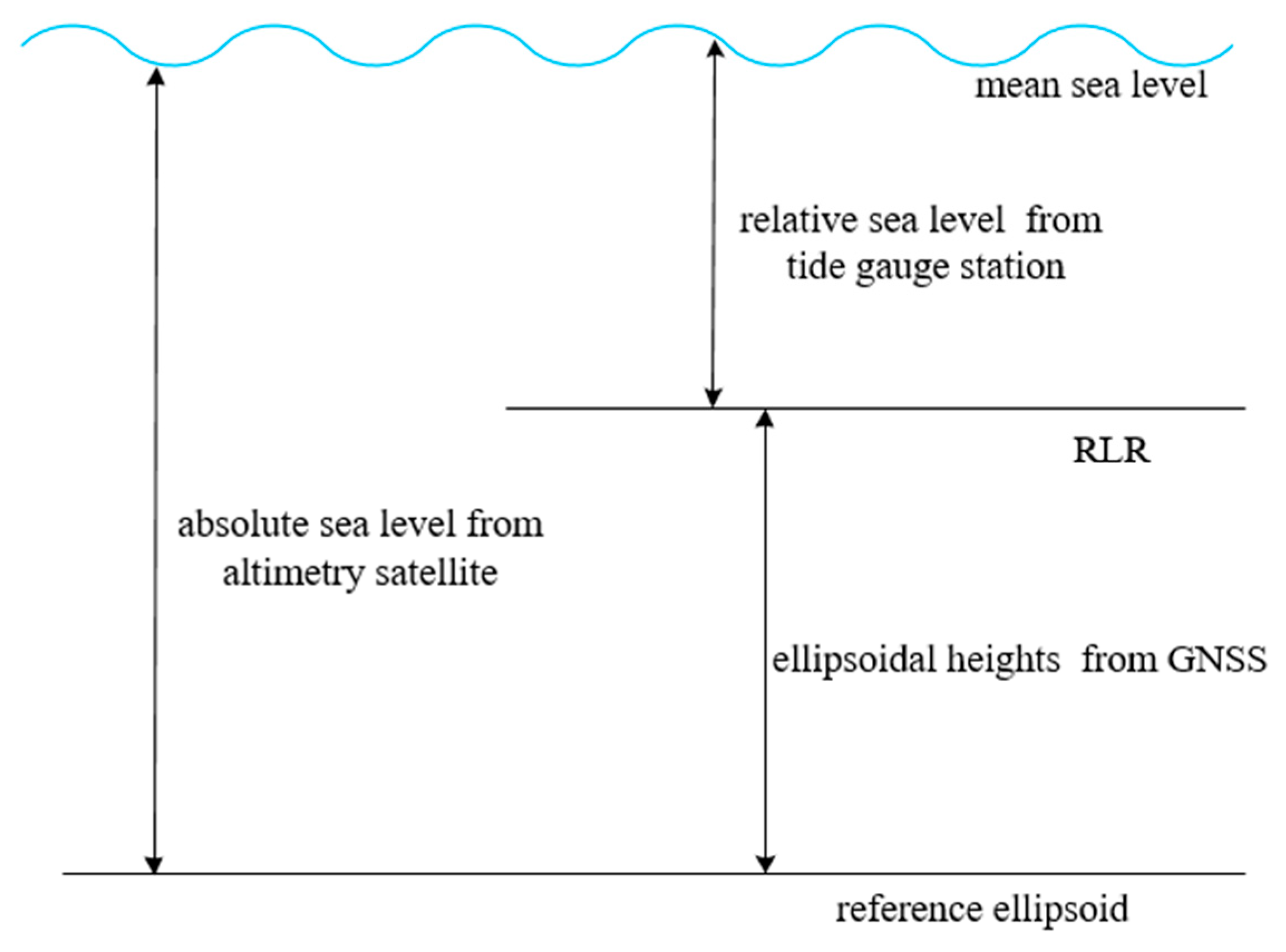
The sea level measured by satellite altimeter is relative to the reference ellipsoid. However, the sea level observed from the tide gauges is relative to a certain benchmark. Therefore, there are differences between these two surfaces. Fortunately, the ellipsoidal height of the benchmark can be obtained by GNSS (equipped on the tide gauges) observation, which can be used to unify the sea level obtained by the tide gauges to the reference ellipsoid. Figure 2 shows the relationship between the sea level measured from the satellite altimeter relative to the reference ellipsoid, the sea level measured from the tide gauges relative to a certain benchmark, and the height of the benchmark measured from GNSS relative to the reference ellipsoid.
The GNSS data downloaded from Systèmed’ Observation duNiveau des Eaux Littorales (SONEL) is the last solution, named ULR6, completed by the University of La Rochelle (ULR) with GAMIT/GLOBK software. Its reference ellipsoid and frame are GRS80 and ITRF08, respectively, and the baseline processing strategy has been detailed in Santamaria-Gomez et al. [32,33]. For information about GNSS stations, refer to Appendix B. GNSS time series data have made corresponding data corrections [32,33] for earthquakes and other emergencies, and the data over three-times larger than the standard deviation have been eliminated by an iterative outlier detection. Then, the eliminated data are filled by the method of SSA iterative interpolation [30,31]. Since the tide gauge records are the annual records, the GNSS daily data for each year are added and averaged as the GNSS annual data for that year for maintaining the consistency of the time scale between the tide gauge records and GNSS measurements.

2.3. Methodology

In this study, the MSS model solely established from multi-satellite altimeter data was established based on the following steps: data selection and preprocessing, collinear adjustment of ERM data, removal of the temporal oceanic variability of GM data, crossover adjustment, and gridding. The 19-year moving average method was used for establishing the MSS model from multi-satellite altimeter data, and then the tide gauge records and joint GNSS data were used to correct the SSH of the MSS model in the offshore area (e.g., 10 km from the coastline).

2.3.1. Collinear Adjustment of Exact Repeat Mission (ERM) Data

After precise data editing and preprocessing, the SSHs obtained by satellite altimeter had higher accuracy. However, the instantaneous SSHs still had large fluctuations and contained temporal oceanic variability signals. A collinear adjustment of the ERM data effectively eliminated the temporal oceanic variability of the SSHs with a period shorter than the period of the collinear tracks used and weaken the sea level anomalies (SLA) caused by large-scale ocean anomalies (such as El Niño and La Niña) in a specific period.
One of the collinear tracks with maximum observations was selected as the reference track. After the reference tracks were determined, the SSH of each point of the collinear tracks corresponding to the point of the reference track was computed by collinear adjustment. The method of collinear adjustment used in our study was the same as that described in Jiang et al. [16] and Jin et al. [17] and it was also used to calculate the mean along-track SSH.
In the process of calculating the mean sea surface height (MSSH), the following steps were implemented [25]: (i) If the difference between SSH and MSSH was larger than 1.0 m, the data were deleted, and the new MSSH was recomputed. (ii) Additionally, it should be ensured that the adjusted data can at least eliminate the time-varying effects of the year, therefore, when the observations participating in the collinear adjustment were less than one year, the point was eliminated.

2.3.2. Temporal Oceanic Variability Corrections of GM Data

Since the GM data did not have the characteristics of repeated cycles, it was impossible to remove the ocean variability by collinear adjustment method. Fortunately, for the period of GM data (e.g., ERS-1/GM span 1994–1995), the ocean variability has been simultaneously observed by ERM data (e.g., T/P span 1994–1995). Therefore, the ocean variability of GM data could be corrected by the ocean variability of the ERM data which was considered as a reference at the spatial and temporal positions of GM data. Altimeter data used for temporal ocean variability corrections of GM data are listed in Table 2. The method of optimal analysis (OA) [10,11] was used in our study. OA was used to interpolate the SLA of one or more missions considered to be a reference at the spatial and temporal position of the satellite that would be corrected for ocean variability.
The altimeter data of T/P, Jason-1, Jason-2, and Jason-3 are acknowledged as having the highest orbit and measuring accuracy. Therefore, the mean along-track SSH of uninterrupted joint T/P + Jason-1 + Jason-2 + Jason-3 (hereafter T/P series) of each group data (shown in Appendix B) was the fundament to calculate the SLA of T/P, Jason-2 and Jason-3. The former was used to correct the ocean variability of a given SSH of GM data.

2.3.3. Crossover Adjustment

Long-wavelength sea level changes of satellite observations can be weakened by collinear adjustment and temporal oceanic variability correction, such as the radial orbit error and the temporal variability of SSH. However, the residual radial orbit error, the short-wavelength signal of temporal oceanic variability and geophysical correction residuals, are still the main influences on the determination of MSS. The crossover adjustment is based on the difference between two observations at the same point to integrate different satellite altimeter data (including ERM data and GM data) or to determine corrections to measurements [25,34,35].
The classical crossover adjustment regards the radial orbit error as one of the dominant sources of errors affecting altimeter data and that error can be sufficiently modelled by either a time- or a distance-dependent polynomial [36,37,38]. With the improvement of the precision orbit determination technology, the radial orbit error of the new generation of satellite altimeter data has been effectively controlled. Therefore, the radial orbit error is no longer the main factor that affects the accuracy of the altimeter data but is a comprehensive effect of the same magnitude as other errors, such as short-wave ocean time-varying signals and geophysical correction residuals.
In this study, the posterior compensation method was used [34,35]. First, the conditional adjustment was used to adjust the crossover observation equation, and then a new error model was used to filter and predict the SSH along the track.
When the condition adjustment is carried out, the SSH at any point along the track can be expressed as:
h = h 0 + Δ ,
where h is the SSH observation, h0 is the true value of h, and Δ is the observation error (systematic error and random error). According to Equation (1), at the crossover point of the track i and j, the conditional equation can be established as:
v i j a v i j d = h i j a h i j d = d i j ,
where dij is the SSH difference at the crossover point. For a track network with multiple crossover points, the matrix form of the crossover point condition equation can be written as:
A V + W = 0 ,
where A is the coefficient matrix, which consists of 1 and −1; V is the correction vector of the observation error, and W is the difference vector of crossover points. The least squares solution of Equation (3) is:
V = P 1 A T ( A P 1 A T ) 1 W ,
and the corresponding cofactor matrix is:
Q V = P 1 A T ( A P 1 A T ) 1 A P 1 ,
where P is the weight matrix of SSH observations. If each observation point on the track is an independent observation, we can derive the following:
{ v i j a = p i j d d i j / ( p i j a + p i j d ) v i j d = p i j a d i j / ( p i j a + p i j d ) ,
where p i j a and p i j d represent the weight factors of observations at the crossover point of the track i and j. In the crossover adjustment of single satellite, p i j a = p i j d = 1 / 2 . In the crossover adjustment of multi-satellite, matrix P is constructed by 1 / 2 times STD of the single-satellite crossover differences.
The comprehensive effect of residuals changes is very complicated, including parts that change linearly and parts that change periodically, and more are parts that have more complicated changes. According to Wagner [36] and Rummel [37], the traditional error model was extended to the following mixed polynomial model with respect to the observed time as the independent variable [35]. It can be expressed as
f ( t ) = a 0 + a 1 ( t T 0 ) + i = 1 m ( b i cos i w ( t T 0 ) + c i sin i w ( t T 0 ) ) ,
where t is the observed time of SSH; a 0 , a 1 , b 1 , and c i ( i = 1 , 2 , , m ) are the undetermined coefficients to be evaluated, and m is a positive integer which is determined with the length of the track. Here, m is proposed to be 1~2 for a short track, 3~5 for a middle-long track, and 6~8 for a long track by experience [35]; w represents the angular frequency corresponding to the periodic change of the error, which can generally be expressed as:
w = 2 π / ( T 1 T 0 ) ,
where T 0 and T 1 represent the corresponding observation times at the beginning and end of the track, respectively.
After the conditional adjustment, V can be regarded as a kind of virtual observation vector. Equation (7) is used as the error model, and then an error equation can be established at the crossover point. This error equation is the following:
v = f ( t ) + δ ,
where v is the virtual observations and δ is the correction of the virtual observations. The matrix form of Equation (9) is as follows:
V   =   B X l ,
where l is the correction vector of the virtual observations; B is a matrix of known coefficients; X is the vector of the undetermined coefficient; and V is the virtual observation vector. The least squares solution of Equation (10) is as follows:
X ^   =   ( B T P V B ) 1 B T P V l ,
where P V is the weight matrix of virtual observations.
The estimated parameter vector X ^ is put into Equation (7). According to the observation time of the along-track SSH of the track, the residuals of SSH systematic error can be calculated and corrected by using Equation (7).

2.3.4. Least-Squares Collocation Technique for Gridding

Most of the orbital errors and residual temporal oceanic variability errors are weakened by the crossover adjustment. However, the differences at the crossover point after adjustment indicate that there is still residual error, especially the GM observations. The least-squares collocation (LSC) technique for gridding can effectively use the prior information of the observations to solve the optimal estimate of the interpolated value [39,40], that is, different weights are given according to the residual error after adjustment to reduce the impact on the accuracy of the SSH.
When using the LSC to grid the SSH, the signal must have a zero-mean characteristic [17,25]. Therefore, the reference MSS model must first be removed from the satellite altimeter data after crossover adjustment. In this study, the CLS15 MSS model in the L2P data product was selected as the reference MSS model. Then, the residual SSH was gridded. Before gridding, the average of the residual SSH should be subtracted to satisfy the zero-mean characteristic. Finally, the MSS model was obtained by adding the grid value to the average and restoring the removed reference MSS model.
Suppose a certain observation vector y contains a zero mean signal t and a zero-mean noise vector v and is expressed as:
y = t + v ,
where the self-covariance matrices of t and v are C t t and C v v , respectively; there is no correlation between t and v, that is, C t v = 0 . Using the LSC technique, for any zero-mean signal s in the data distribution, the fitted value [17] is:
s ^ = C s t ( C t t + C v v ) 1 y ,
where C s t is the cross-covariance between signal s and signal t, and again, there is no correlation between s and v. If the self-covariance C s s of the signal s is known, the estimation error of s can be expressed as:
E s ^ s ^ = C s s C s t ( C t t + C v v ) 1 C s t T .
When the fitting point and the observation point coincide, the observation point is considered to have no error, that is, C s t = C t t = C s s , C v v = 0 . From Equations (13) and (14), the estimated value s ^ = t and the error E s ^ s ^ = 0 satisfy the general interpolation method. Therefore, when the cross-covariance between the a priori information and the signal as well as the error is accurately known, LSC can effectively use the a priori information of the observations to obtain accurate interpolation values.
Because the satellite altimeter observations are very large and the data around each network point are densely distributed, they are insensitive to the accuracy of the covariance function when determining the MSSH of each network point [41]. Therefore, a second-order Markov process was used to describe the one-dimensional covariance function [42]. The process can be expressed as [43]:
cov ( d ) = C 0 ( 1 + d / α ) e d / α ,
where d is the two-dimensional distance between the observation point and the grid point; C 0 is the local variance parameter, which can be expressed by the variance of all observations in the local range involved in the grid. α = 0.595 ξ , α is the parameter to be estimated and ξ is the correlation length (where a 50% correlation is obtained) [44], and the value is 70 km [45,46]. The single-satellite crossover differences accuracy of 1 / 2 times after the crossover adjustment is introduced into the LSC as the noise of the corresponding satellite data.

2.3.5. Nineteen-Year Moving Average Method

Almost all altimeter data from 1993 to 2018 with a period of 26 years were used in the establishment of the MSS model. To further eliminate the influence of the residual errors of tide model error on the altimeter data (in Table 1), these data were put into 8 groups over 19-year-long moving windows, starting in 1993 and shifted by one year. The 8 sets of data were independently established an MSS model, respectively, and eight MSS models were obtained. Then, the final MSS model was determined by calculating the average at each grid point of these eight MSS models.
Also, the SSHs (span 1993–2018) obtained from the corrected tide gauge records and the joint GNSS data were grouped with the same method used in altimeter data. In this way, eight groups SSHs of each tide gauge station (a total of 28 tide gauges) at different periods were obtained. Then, the average value of the 8 SSHs of the tide gauges was calculated for the SSH of that tide gauge, and used to correct the SSHs of the MSS model in the offshore region.
The calculating process is described as follows [25]:
S S H i , s = j 8 s s h i , j / 8 ,
where S S H i , s is the SSH at the grid point i in the SJAO2020A (see Section 3.1.3) model or at the i-th of the 28 tide gauges, and s s h i , j is the SSH at the grid point i in each of the eight models or the SSH of the eight groups SSH of the i-th tide gauge.
The mean along-track SSH of uninterrupted joint T/P series over the period of each group was used as fundament, for example, the mean along-track SSH of uninterrupted joint T/P series during 1992–2011 was the fundament for the first MSS model. The SJAO2020A model was derived from the average of eight MSS models. Therefore, the fundament for SJAO2020A model was the average of the fundaments for the eight MSS models, i.e., the mean along-track SSH of uninterrupted joint T/P series during 1993–2018 could be considered to be the fundament for the SJAO2020A model.

2.3.6. The Method for Improving the Coastal Accuracy of the Model

First, inverse barometer correction was performed on the tide gauge records, after preprocessing described earlier. Then, the SSHs (span 1993–2018) obtained from the corrected tide gauge records and the joint GNSS data were adjusted to have the same reference ellipsoid and frame as T/P. Finally, the SSH of each tide gauge station was obtained with the 19-year moving average method. These SSHs were used to correct the SSHs of the grid points of the SJAO2020A model within 10 km from each tide gauge station. Regarding why the data of 10 km away from the coastline was selected to be corrected, please see Appendix C for specific reasons.
The method of Gaussian inverse distance weighting was used in the process of the corrections. The correction value Δ h of each grid point is expressed as:
Δ h = ( H t i d e H s s h ) × p ,
where H t i d e is the tide gauge SSH, H s s h is the SSH of the grid point of the SJAO2020A model within 10 km from each tide gauge station, and p is a weighting factor weighted by the Gaussian inverse distance, which can be expressed as:
p = e d 2 α 2 ,
where α is the Gaussian distance smoothing factor, which is 10 km in this study and d is the spherical distance from the grid point to the tide gauge station. The calculation equation is:
R = a × 1 e 2 / ( 1 e 2 × sin 2 ( ( y t + y s ) / 2 ) ) ,
d = 2 × R × sin 2 ( Δ y ) + cos ( y t ) × cos ( y s ) × sin 2 ( Δ x ) ,
where a is the semimajor axis of the T/P reference ellipsoid; y t and x t are the latitude and longitude of the tide gauge station; y s and x s are the latitude and longitude of the grid point; and Δ y = ( y t y s ) / 2 , and Δ x = ( x t x s ) / 2 .
Finally, in the study area, the correction of the coastal (10 km from the coastline) grid points of the MSS model was realized by the spline interpolation method [47] of adjustable tensor continuous curvature in the Generic Mapping Tools (GMT) software [48].

3. Results and Analysis

3.1. Establishment of the MSS Model Based on Satellite Altimeter

3.1.1. Correction of Temporal Oceanic Variability

To validate the effect of correction of temporal oceanic variability, the crossover differences of SSH before and after temporal oceanic variability correction are separately counted. The statistical results are shown in Table 3.
Table 3 shows that the accuracy of the ERM data is greatly improved after collinear adjustment. This shows that the temporal oceanic variability signal has a significant influence on the MSS. Collinear processing can weaken the effect of temporal oceanic variability on ERM data and improve (better than 10 cm) the calculation accuracy of the SSH. The T/P series, as the spatial-temporal fundamental, has the highest accuracy of crossover differences. According to Table 2, temporal oceanic variability correction is performed on the GM data. The effect of temporal oceanic variability correction is shown in Table 3, in which the crossover difference is improved by approximately 7 cm.

3.1.2. The Results of the Crossover Adjustment

In the crossover adjustment of multi-satellite, the mean along-track SSH of uninterrupted joint T/P series is used as fundament. Satellite observations with high orbit accuracy improve that with low orbit accuracy by combining all satellite data with the method of crossover adjustment. The combined effects of the above radial orbit errors and other errors are further eliminated, realizing the unity and coordination of the combined processing of multiple satellite altimeter data.
It can be seen from Table 3 and Table 4 that after the self-crossover adjustment between the satellites, the STD of the crossover difference of SSH in ERM data is at the level of 1~4 cm and the GM data is approximately 9 cm, which effectively reduces the residual radial orbit errors of each satellite. The STD of the crossover difference after the joint crossover adjustment of each satellite is 0.0811 m, realizing the improvement of satellite observations with high accuracy to the satellite observations with low accuracy. The T/P series data are used as fundament, and the STD of the self-crossover difference is 0.0068 m, which is smallest as compared with other satellites. Therefore, it is still in a dominant position in the joint crossover adjustment, and the coordination between multiple satellites is achieved, while the benchmark is unchanged.

3.1.3. Establishment of the Model

The LSC method is a statistical estimation method based on the observation covariance information that takes full account of the statistical correlation between the data; the smoothing function is better than Shepard, continuous curvature tension spline, and other analytical methods, and therefore it is more suitable to grid satellite altimeter along-track data after crossover adjustment [17]. Eight MSS models are obtained from the eight groups of altimeter data in Table A1. The MSS model over the Sea of Japan and its adjacent ocean was determined from multi-satellite altimeter data (named SJAO2020A) by taking the average at the grid point of these eight MSS modes. To validate the accuracy of the SJAO2020A model, it is compared with DTU18, DTU15, Whu13, CLS15, and CLS11 within different distances from the coastline, respectively. The STD of the differences of the SSH between SJAO2020A and DTU18, DTU15, Whu13, CLS15, and CLS11, within 10 km, 10–20 km, 20–30 km, 30–40 km, and 40–50 km from the coastline, are shown in Figure 3.
It can be seen from Figure 3 that the STDs of the differences of the SSH between SJAO2020A and CLS15 are always the smallest, and the largest is that of CLS11. The CLS11 model was established using only the satellite data from 1993 to 2009, and the GM data were only used from the ERS-1 satellite from 1994 to 1995. The STD of the difference between SJAO2020A and the other four models decreases with increasing distance from the coastline, and the largest decrease is within the range of 10~20 km. After 40 km, the STD is relatively stable, at approximately 0.025 m, indicating that the accuracy of SJAO2020A is relatively stable and reliable. However, these MSS models are very different in coastal areas, which is caused by the low coastal accuracy of satellite altimeter data. Therefore, improving the coastal accuracy of SSH is extremely important for improving the overall accuracy of the MSS model. In this study, the coastal accuracy of SJAO2020A was improved using 24 tide gauge stations and joint GNSS around the Japanese coastline.

3.2. Improvement of Model Coastal Accuracy

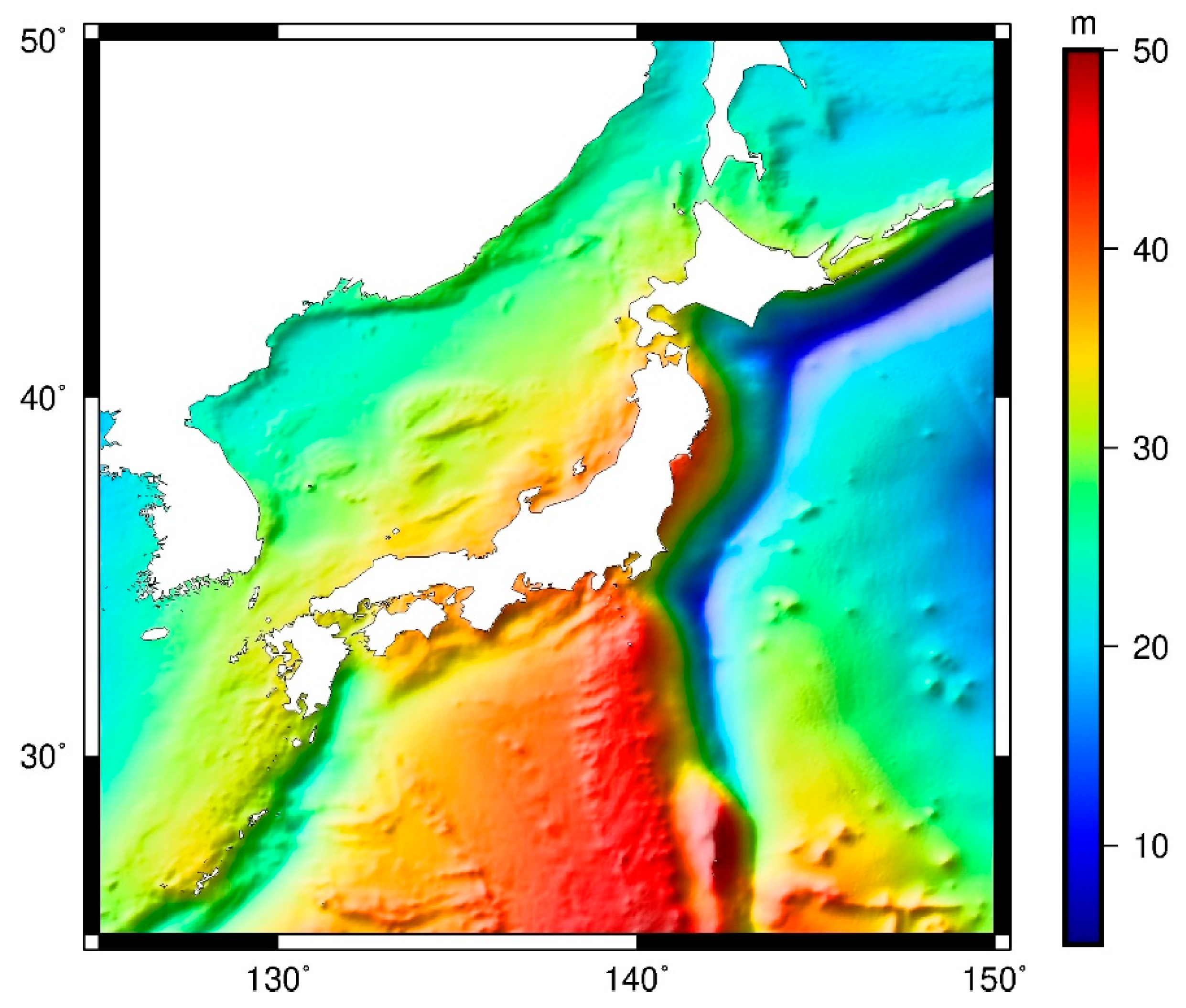
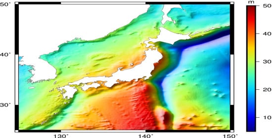
The Gaussian inverse distance weighting method was used to correct the SSH of grid points within 10 km from the 24 tide stations. Then, the adjustable tensor continuous curvature spline interpolation method was used to correct all coastal grid points of SJAO2020A. The final MSS model (reference to T/P reference ellipsoid) over the Sea of Japan and its adjacent ocean (named SJAO2020) was established, as shown in Figure 4.
Figure 4 shows that the SSH change over the Sea of Japan and its adjacent ocean areas is complicated. The overall SSH of the Philippine plate is higher than that of the Pacific plate. Among them, the SSH of the Izu-Ogasawara Trench, Japan Trench, and Thousand Islands Trench is low. The lowest point is the Thousand Islands Trench, which is −2.826 m. The highest point at SSH is 52.9643 m, near the Ogasawara Islands.
To verify the coastal accuracy of SJAO2020 corrected by the tide gauge station, the SSHs of DTU18, CLS15, SJAO2020, and SJAO2020A at the position of the tide gauge station (the red solid circle in Figure 1) were interpolated and compared with the actual measured SSHs of the tide gauge stations. The statistical results are shown in Table 5.
In Table 5, H D T U 15 and H C L S 15 represent the SSH at the tide gauge station calculated by DTU18 and CLS15 model, respectively. H S J A O 2020 A and H S J A O 2020 represent the SSH at the tide gauge station calculated by SJAO2020A and SJAO2020, respectively. DTU18 and CLS15 are a few centimeters away from the sea level at tide gauge stations Ogi, Ito II, and Kushimoto, and are about 4 dm away from the sea level at tide gauge station Tajiri, while the sea level difference between SJAO2020a and tide gauge station Tajiri is about 4 cm. The SSH difference between SJAO2020 and the four tide gauge stations is approximately 2 cm, which improves the SSH difference between SJAO2020A and the tide station. This indicates that the Gaussian inverse distance weighting method based on tide gauge stations and the joint GNSS can effectively improve the coastal accuracy of the SJAO2020 MSS model.

3.3. Accuracy Assessment of SJAO2020

Usually, reliability and accuracy are validated by comparing with mean along-track altimetry data and other models [1]. The difference between MSS models depends on the dataset used for calculation and the data processing method [11]. To evaluate the model error of SJAO2020 at different wavelength scales and to better quantify the difference between it and DTU18, DTU15, CLS15, CLS11, and WHU13, based on the mean along-track ERM data of the one-year uninterrupted Sentinel-3B satellite in 2019, the along-track SLAs between the Sentinel-3B and SJAO2020, DTU18, DTU15, CLS15, CLS11, and WHU13 models were obtained. The power spectral density (PSD) of the along-track SLA in different wavelength ranges were obtained by using the fast Fourier transform (FFT). The Sentinel-3B data used in this study was completely independent of all models, whether time or satellite ground tracks.
As shown in Figure 5a, the error of each model is obviously different for wavelengths longer than 300 km. This is due to the independence of each model and the systematic error between each model included in the SLA time series. Among them, the systematic error between SJAO2020 and DTU18, as well as CLS15, is relatively small due to the types and quantities of SSH data used by the three are the closest. The error of each model drops rapidly at wavelengths of 250~300 km. At wavelengths of 35~250 km, the SJAO2020 error is significantly improved as compared with other models. In the smaller wavelength range of 12~18 km, the errors of each model have a small increase, of which satellite altimeter noise is dominant [12]. Figure 5b shows the ratio of the along-track PSD of DTU15, DTU18, and CLS15 in Figure 5a to the along-track PSD of SJAO2020. Compared with DTU18 and DTU15, the SLA change of SJAO2020 is reduced by 11.76% and 59.24%, respectively in the wavelength range of 35~300 km, and the improvement is greatest when the wavelength is 66 km. The SLA change of SJAO2020 is reduced by 8.91% as compared with CLS15 in the wavelength range of 35~300 km.
As seen from the above, satellite altimeter data are also an effective method for evaluating the MSS model. The SLA of satellite altimeter data and five models were obtained separately. Among them, the satellite altimeter data include collinear data of the T/P series, ERS-1, HY-2A, and Sentinel-3B, as well as GM data of Jason-2 and SRL (due to technical problems, the SRL satellite drifted in repetitive periodic tracks in March 2015; compared with historical repetitive tracks, the maximum drift amount is up to 10 km). The root mean square error of each SLA in the wavelength range of 35 to 300 km was calculated by Chebyshev bandpass filtering. The statistical results are shown in Table 6.
As shown in Table 6, the STD of the SLA given by SJAO2020 and its benchmark (T/P series) data in the wavelength range of 35 to 300 km is the smallest as compared with the other five models, indicating that the model is the most stable and the data processing results are more reliable. The STD of the along-track SLA given by between HY-2A and SJAO2020 is significantly smaller than that of the other five models. This is because HY-2A data are only used in SJAO2020, indicating that the accuracy of the MSS model at the ground track of the satellite can be improved by adding more high accuracy satellite observations. Sentinel-3B, SRL, and Jason-2/GM are not used in the establishment of the SJAO2020, CLS15, DTU18, DTU15, WHU13, and CLS11 models, and the STDs of the three-satellite data along-track SLA are sequentially reduced. This shows that the accuracy of the SJAO2020 model is the highest. The accuracy of CLS15 is equivalent to that of DTU18. As compared with DTU15, the accuracy of DTU18 has been improved, and the accuracy of both models is better than WHU13. However, the ERS-1 along-track data are consistent with CLS11, only second to SJAO2020, and better than CLS15, DTU18, DTU15, and WHU13. This may be caused by the establishment of the CLS11 model using only the GM data of one ERS-1 satellite. The model has a strong correlation with the ERS-1 satellite.

4. Conclusions

A new MSS model named SJAO2020A with a grid of 1′ × 1′ over the Sea of Japan and its adjacent ocean was established with the 19-year moving average method by combining satellite altimeter data from 1993 to 2018. Different from the latest MSS models CLS15 and DTU18, the measured data of the latest altimetry satellites HY-2A, Jason-3, and Sentinel-3A are ingested in SJAO2020A. To improve the coastal accuracy of SJAO2020A, 24 tide gauges and the joint GNSS stations along the coast of Japan are used to correct the sea surface height within 10 km from the coastline by using the Gaussian inverse distance weighting method. Then, the SJAO2020 model with higher coastal accuracy is obtained. The difference between SJAO2020 and the four tide gauge stations (the red solid circle in Figure 1) is approximately 2 cm, and SJAO2020 coastal accuracy is better than that of CLS15 and DTU18.
To better quantify the differences among the MSS models (SJAO2020, DTU18, DTU15, CLS15, CLS11, and WHU13), this study obtained the power spectral density of the along-track sea level anomalies (SLA) between Sentinel-3B and these models. The SLA change of SJAO2020 is 11.76% and 59.24% lower than that of DTU18 and DTU15 in the wavelength range of 35~300 km, respectively. Through the STD analysis of the along-track SLA between different satellite data and each model in the wavelength range of 35 to 300 km, the SJAO2020 model has the smallest error and improved several millimeters. This shows that the method proposed in this study is effective for improving the accuracy of the SSH of the MSS model in the offshore region.

Author Contributions

Conceptualization, J.G.; Data curation, J.Y.; Formal analysis, J.Y., Y.N., C.Z., and Z.L.; Funding acquisition, J.G.; Investigation, J.Y., Y.N., C.Z., and Z.L.; Methodology, J.Y., J.G., Y.N., C.Z., and Z.L.; Project administration, J.G.; Resources, J.Y. and J.G.; Software, J.Y. and Y.N.; Supervision, J.G.; Validation, Y.N. and C.Z.; Visualization, Y.N. and Z.L.; Writing—original draft, Y.N.; Writing—review and editing, J.Y. All authors have read and agreed to the published version of the manuscript.

Funding

This research was funded by the National Natural Science Foundation of China (grant nos. 41774001 and 41374009), the SDUST Research Fund (grant no. 2014TDJH101), and the Autonomous and Controllable Special Project for Surveying and Mapping of China (grant no. 816-517).

Acknowledgments

We thank Ole Andersen for helpful discussions and proposals. We are very grateful to AVISO+ for providing the along-track L2P products and the waveform data of Jason-1, which can be obtained by downloading freely from AVISO+ official website (ftp://ftp-access.aviso.altimetry.fr). The tide gauge records are available online (https://www.psmsl.org/) and the GPS data are available online (https://www.sonel.org).

Conflicts of Interest

The authors declare no conflict of interest.

Appendix A

Table A1. Information of the 28 tide gauges.
Tide GaugeLongitude LatitudeMissing Rate of RecordsRLR 1 (m)Tide GaugeLongitude LatitudeMissing Rate of RecordsRLR 1 (m)
Wakkanai141.685
45.407
019.9807Aburatsubo139.615
35.160
028.8722
Abashiri144.285
44.019
0.137%23.2246Katsuura140.249
35.129
0.137%26.2751
Oshoro II140.858
43.209
025.7054Hamada II132.066
34.897
026.6065
Kushiro144.371
42.975
022.2085Onisaki136.823
34.903
031.0473
Hakodate I140.724
41.781
027.3744Yaizu138.327
34.870
0.137%33.1441
Asamshi140.859
40.897
0.137%30.0906Mera139.825
34.918
029.3934
Oga139.705
39.942
0.137%306029Ito II139.133
34.895
033.3934
Ogi138.281
37.814
031.1457Tago138.764
34.806
0.137%33.3729
Kashiwazaki138.508
37.356
0.275%32.1022Kainan135.191
34.144
031.2235
Wajima136.901
37.405
030.4164Kure I133.243
33.333
029.1527
Toyama137.224
36.762
031.2808Kushimoto135.773
33.475
031.8860
Mikuni136.148
36.254
029.3105Nagasaki129.866
32.735
025.6219
Tajiri134.315
35.593
028.8719Hosojima131.669
32.428
0.137%22.7373
Aburatsu131.409
31.576
021.3963Naha127.665
26.213
024.5357
1 The ellipsoidal heights of the revised local reference (RLR) of the tide gauge.

Appendix B

Table A2. GNSS data information.
GNSS StationReceiver INFORMATIONAntenna InformationTotal Number of Sessions
P101TRIMBLE 5700/TPS NETG3/TPS NET-G5TRM29659.00 DOME3732
P103TRIMBLE 5700/TPS NETG3/TPS NETG5TRM29659.00 DOME3849
P104TRIMBLE 5700/TPS NETG3/TPS NETG5TRM29659.00 DOME3754
P107TRIMBLE 5700/TRIMBLE NetRS/TPS NETG3/TPS NET-G5TRM29659.00 DOME3762
P108TRIMBLE 5700/TPS NETG3/TPS NET-G5TRM29659.00 DOME3838
P109TRIMBLE 5700/TPS NETG3/TPS NETG5TRM29659.00 DOME3783
P110TRIMBLE 5700/TPS NETG3/TPS NETG5TRM29659.00 DOME3711
P111TRIMBLE 5700/TPS NETG3/TPS NET-G5TRM29659.00 DOME3762
P112TRIMBLE 5700/TPS NETG3/TPS NETG5TRM29659.00 DOME3768
P113TRIMBLE 5700/TPS NETG3/TPS NETG5TRM29659.00 DOME3730
P114TRIMBLE 5700/TPS NETG3/TPS NETG5TRM29659.00 DOME3734
P115TRIMBLE 5700/TRIMBLE NetRS/TPS NETG3/TPS NETG5TRM29659.00 DOME3741
P116TRIMBLE 5700/TPS NETG3/TPS NETG5TRM29659.00 DOME3762
P117TRIMBLE 5700/TPS NETG3/TPS NETG5TRM29659.00 DOME3754
P118TRIMBLE 5700/TPS NETG3/TPS NETG5TRM29659.00 DOME3706
P120TRIMBLE 5700/TPS NETG3/TPS NETG5TRM29659.00 DOME3753
P122TRIMBLE 5700/TPS NETG3/TPS NETG5TRM29659.00 DOME3785
P201TRIMBLE 5700/TPS NETG3/TPS NETG5TRM29659.00 DOME3764
P202TRIMBLE 5700/TPS NETG3/TPS NETG5TRM29659.00 DOME
TRM59800.80 DOME
3733
P203TRIMBLE 5700/TPS NETG3/TPS NETG5TRM29659.00 DOME
TRM59800.80 DOME
3802
P204TRIMBLE 5700/TPS NETG3/TPS NETG5TRM29659.00 DOME
TRM59800.80 DOME
3781
P206TRIMBLE 5700/TPS NETG3/TPS NETG5TRM29659.00 DOME3734
P207TRIMBLE 5700/TPS NETG3/TPS NETG5TRM29659.00 DOME3731
P208TRIMBLE 5700/TPS NETG3/TPS NETG5TRM29659.00 DOME3794
P209TRIMBLE 5700/TPS NETG3/TPS NETG5TRM29659.00 DOME
TRM59800.80 DOME
3367
P210TRIMBLE 5700/TPS NETG3/TPS NETG5TRM29659.00 DOME
TRM59800.80 DOME
3765
P211TRIMBLE 5700/TPS NETG3/TPS NETG5TRM29659.00 DOME
TRM59800.80 DOME
3394
P212TRIMBLE 5700/TPS NETG3/TPS NETG5TRM29659.00 DOME
TRM59800.80 DOME
3708

Appendix C

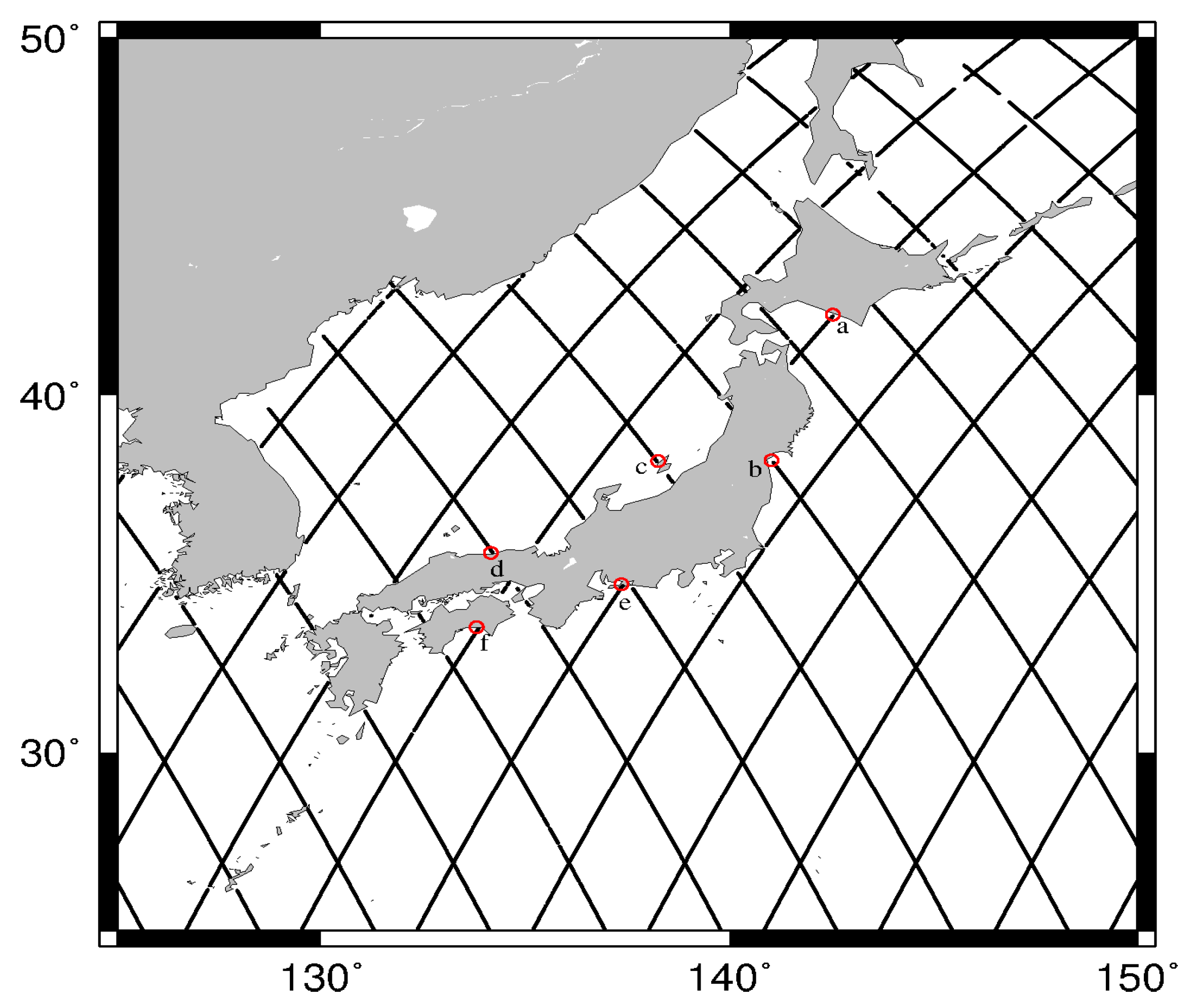
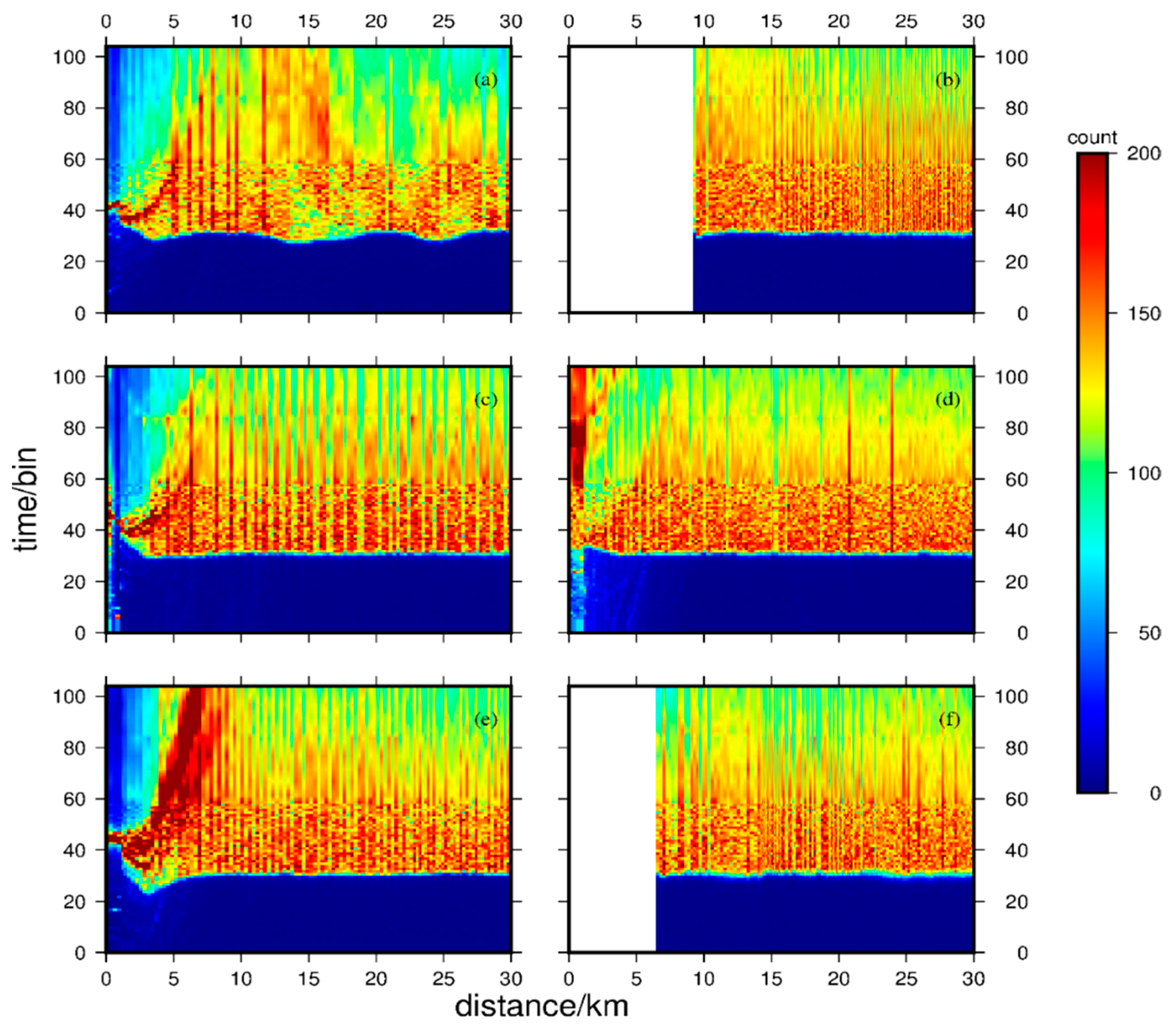
Altimeter waveforms are usually contaminated due to land, island, sea reef, sea ice, seabed terrain, etc. If the extracted ranges from these corrupted waveforms are used, sea levels calculated from these ranges are also incorrect [20]. However, for the seas of Japan and its adjacent ocean, how far away from the coastline is the altimeter data that is incorrect and cannot be used? To solve this question, six arcs (Figure A1) of Jason-1 satellite from sea to land or from land to sea are selected from the study area. The return power of each arc within 30 km from the coastline is shown in Figure A2.
Figure A1. Ground tracks of Jason-1 and geographical distribution of waveform data.
Remotesensing 12 04168 g0a1
Figure A2. Return power for each selected arc. Here a-f are the return power of a-f arcs in Figure A1.
Remotesensing 12 04168 g0a2
As shown in Figure A2a,c–e, the waveforms of Jason-1 began to be contaminated approximately 10 km from the coastline. The closer the waveform is to the coastline, the more serious the waveform is contaminated and the greater the accuracy of sea level observations. There is no obvious waveform contamination of arcs b and f in cycle 18, but the two arcs only have waveform data after 9.361 km and 6.596 km from the coastline. Therefore, the tide gauge stations are mainly used to correct the SSH of the MSS model 10 km away from the coastline.

References

  1. Andersen, O.B.; Knudsen, P. DNSC08 mean sea surface and mean dynamic topography models. J. Geophys. Res. Ocean. 2009, 114, 327–432. [Google Scholar] [CrossRef]
  2. Qiu, H.; Jin, S. Global Mean Sea Surface Height Estimated from Spaceborne Cyclone-GNSS Reflectometry. Remote Sens. 2020, 12, 356. [Google Scholar] [CrossRef] [Green Version]
  3. Zhu, C.; Guo, J.; Hwang, C.; Gao, J.; Yuan, J.; Liu, X. How HY-2A/GM altimeter performs in marine gravity derivation: Assessment in the South China Sea. Geophys. J. Int. 2019, 219, 1056–1064. [Google Scholar]
  4. Zhu, C.; Guo, J.; Gao, J.; Liu, X.; Hwang, C.; Yu, S.; Yuan, J.; Ji, B.; Guan, B. Marine gravity determined from multi-satellite-GM/ERM altimeter data over the South China Sea: SCSGA V1.0. J. Geod. 2020, 94, 50. [Google Scholar] [CrossRef]
  5. Guo, J.; Wang, J.; Hu, Z.; Liu, X.; Kong, Q.; Zhao, C. Vertical land movement over China coasts determined by tide gauge and satellite altimetric data. Arab. J. Geosci. 2016, 9, 168. [Google Scholar] [CrossRef]
  6. Guo, J.; Wang, J.; Hu, Z.; Hwang, C.; Chen, C.; Gao, Y. Temporal-spatial variations of sea level over Chinese seas derived from altimeter data of TOPEX/Poseidon, Jason-1 and Jason-2 from 1993 to 2012. Chin. J. Geophys. Chin. Ed. 2015, 58, 3103–3120. [Google Scholar]
  7. Dufau, C.; Orstynowicz, M.; Dibarboure, G.; Morrow, R.; La Traon, P.-Y. Mesoscale resolution capability of altimetry: Present & future. J. Geophys. Res. Ocean. 2016, 121, 4910–4927. [Google Scholar]
  8. Marsh, J.G.; Koblinsky, C.J.; Zwally, H.J.; Brenner, A.C.; Beckley, B.D. A global mean sea surface based upon GEOS 3 and Seasat altimeter data. J. Geophys. Res. 1992, 97, 4915–4921. [Google Scholar] [CrossRef]
  9. Hernandez, F.; Schaeffer, P. The CLS01 Mean Sea Surface: A Validation with the GSFC00.1 Surface; CLS: Ramonville St Agne, France, 2001. [Google Scholar]
  10. Schaeffer, P.; Ollivier, A.; Faugere, Y.; Bronner, E.; Picot, N. The new CNES CLS 2010 mean sea surface. In Proceedings of the Oral Presentation at OSTST Meeting, Lisbon, Portugal, 18–22 October 2010; pp. 21–22. [Google Scholar]
  11. Schaeffer, P.; Faugére, Y.; Legeais, J.F.; Ollivier, A.; Guinle, T.; Picot, N. The CNES_CLS11 Global Mean Sea Surface Computed from 16 Years of Satellite Altimeter Data. Mar. Geod. 2012, 35, 3–19. [Google Scholar] [CrossRef]
  12. Pujol, M.-I.; Schaeffer, P.; Faugère, Y.; Raynal, M.; Dibarboure, G.; Picot, N. Gauging the improvement of recent mean sea surface models: A new approach for identifying and quantifying their errors. J. Geophys. Res. Ocean. 2018, 123, 5889–5911. [Google Scholar] [CrossRef]
  13. Andersen, O.B.; Knudsen, P.; Stenseng, L. The DTU13 MSS (mean sea surface) and MDT (mean dynamic topography) from 20 years of satellite altimetry. In Proceedings of the 3rd International Gravity Field Service (IGFS), Shanghai, China, 30 June–6 July 2014; Jin, S., Barzaghi, R., Eds.; Springer: Cham, Switzerland, 2015; Volume 144, pp. 111–121. [Google Scholar]
  14. Andersen, O.B.; Piccioni, G.; Stenseng, L.; Knudsen, P. The DTU15 MSS (mean sea surface) and DTU15LAT (lowest astronomical tide) reference surface. In Proceedings of the ESA Living Planet Symposium 2016, Prague, Czech Republik, 9–13 May 2016. [Google Scholar]
  15. Andersen, O.B.; Knudsen, P.; Stenseng, L. A new DTU18 MSS mean sea surface—Improvement from SAR altimetry. 172. In Proceedings of the 25 Years of Progress in Radar Altimetry Symposium, Ponta Delgada, São Miguel Island, Azores Archipelago, Portugal, 24–29 September 2018; Volume 172, pp. 24–26. [Google Scholar]
  16. Jiang, W.; Li, J.; Wang, Z. Determination of global mean sea surface WHU2000 using multi-satellite altimetric data. Chin. Sci. Bull. 2002, 47, 1664–1668. [Google Scholar] [CrossRef]
  17. Jin, T.Y.; Li, J.C.; Jiang, W.P.; Wang, Z.T. The new generation of global mean sea surface height model based on multi-altimetric data. Acta Geod. Et Cartogr. Sin. 2011, 40, 723–729. [Google Scholar]
  18. Jin, T.Y.; Li, J.C.; Jiang, W.P. The global mean sea surface model WHU2013. Geod. Geodyn. 2016, 7, 202–209. [Google Scholar] [CrossRef] [Green Version]
  19. Guo, J.; Gao, Y.; Hwang, C.; Sun, J. A multi-subwaveform parametric retracker of the radar satellite altimetric waveform and recovery of gravity anomalies over coastal oceans. Sci. China Earth Sci. 2010, 53, 610–616. [Google Scholar] [CrossRef]
  20. Yuan, J.; Guo, J.; Niu, Y.; Zhu, C.; Li, Z.; Liu, X. Denoising Effect of Jason-1 Altimeter Waveforms with Singular Spectrum Analysis: A Case Study of Modelling Mean Sea Surface Height over South China Sea. J. Mar. Sci. Eng. 2020, 8, 426. [Google Scholar] [CrossRef]
  21. Menéndez, M.; Woodworth, P.L. Changes in extreme high water levels based on a quasi-global tide-gauge data set. J. Geophys. Res. Oceans 2010, 115, C10011. [Google Scholar] [CrossRef] [Green Version]
  22. Iliffe, J.C.; Ziebart, M.K.; Turner, J.F. A New Methodology for Incorporating Tide Gauge Data in Sea Surface Topography Models. Mar. Geod. 2007, 30, 271–296. [Google Scholar] [CrossRef]
  23. Stammer, D.; Ray, R.D.; Andersen, O.B.; Arbic, B.K.; Bosch, W.; Carrère, L.; Cheng, Y.; Chinn, D.S.; Dushaw, B.D.; Egbert, G.D.; et al. Accuracy assessment of global barotropic ocean tide models. Rev. Geophys. 2014, 52, 243–282. [Google Scholar] [CrossRef] [Green Version]
  24. Carrère, L.; Lyard, F.; Cancet, M.; Guillot, A.; Dupuy, S. FES 2014: A new global tidal model. In Proceedings of the OSTST Meeting, Lake Contance, Germany, 28–31 October 2014. [Google Scholar]
  25. Yuan, J.; Guo, J.; Liu, X.; Zhu, C.; Niu, Y.; Li, Z.; Ji, B.; Ouyang, Y. Mean sea surface model over China seas and its adjacent ocean established with the 19-year moving average method from multi-satellite altimeter data. Cont. Shelf Res. 2020, 192, 104009. [Google Scholar] [CrossRef]
  26. Bird, P. An updated digital model of plate boundaries. Geochem. Geophy. Geosy. 2003, 4, 1027. [Google Scholar] [CrossRef]
  27. Ishii, M.; Kimoto, M.; Sakamoto, K.; Iwasaki, S.-I. Steric sea level changes estimated from historical ocean subsurface temperature and salinity analyses. J. Oceanogr. 2006, 62, 155–170. [Google Scholar] [CrossRef]
  28. CNES. Along-Track Level-2+ (L2P) SLA Product Handbook; SALP-MU-P-EA-23150-CLS, Issue1.0; CNES: Paris, France, 2017.
  29. Holgate, S.J.; Matthews, A.; Woodworth, P.L.; Rickards, L.J.; Tamisiea, M.E.; Bradshaw, E.; Foden, P.R.; Gordon, K.M.; Jevrejeva, S.; Pugh, J. New data systems and products at the permanent service for mean sea level. J. Coast. Res. 2013, 29, 493–504. [Google Scholar]
  30. Hassani, H. Singular spectrum analysis: Methodology and comparison. J. Data Sci. 2007, 5, 239–257. [Google Scholar]
  31. Shen, Y.; Guo, J.; Liu, X.; Kong, Q.; Guo, L.; Li, W. Long-term prediction of polar motion using a combined SSA and ARMA model. J. Geod. 2018, 92, 333–343. [Google Scholar] [CrossRef]
  32. Santamaría-Gómez, A.; Gravelle, M.; Collilieux, X.; Guichard, M.; Míguez, B.M.; Tiphaneau, P.; Wöppelmann, G. Mitigating the effects of vertical land motion in tide gauge records using state-of-the-art GPS velocity field. Global. Planet. Change 2012, 98–99, 6–17. [Google Scholar]
  33. Santamaría-Gómez, A.; Gravelle, M.; Dangendorf, S.; Marcos, M.; Spada, G.; Wöppelmann, G. Uncertainty of the 20th century sea-level rise due to vertical land motion errors. Earth. Planet. Sc. Lett. 2017, 473, 24–32. [Google Scholar] [CrossRef]
  34. Huang, M.; Guan, Z.; Zhai, G.; Ouyang, Y. On the compensation of systematic errors in marine gravity measurements. Mar. Geod. 1999, 22, 183–194. [Google Scholar]
  35. Huang, M.; Zhai, G.; Ouyang, Y.; Lu, X.; Liu, C.; Wang, R. Integrated Data Processing for Multi-Satellite Missions and Recovery of Marine Gravity Field. Terr. Atmos. Ocean. Sci. 2008, 19, 103. [Google Scholar] [CrossRef] [Green Version]
  36. Wagner, C.A. Radial variations of a satellite orbit due to gravitational errors: Implications for satellite altimetry. J. Geophys. Res. Sol. Earth 1985, 90, 3027–3036. [Google Scholar] [CrossRef]
  37. Rummel, R. Principle of satellite altimetry and elimination of radial orbit errors. In Satellite Altimetry in Geodesy and Oceanography; Rummel, R., Sansò, F., Eds.; Springer: Berlin/Heidelberg, Germany, 1993; Volume 50, pp. 190–241. [Google Scholar]
  38. Knudsen, P.; Brovelli, M. Collinear and cross-over adjustment of Geosat ERM and Seasat altimeter data in the Mediterranean Sea. Surv. Geophys. 1993, 14, 449–459. [Google Scholar] [CrossRef]
  39. Wunsch, C.; Zlotnicki, V. The accuracy of altimetric surfaces. Geophys. J. Int. 1984, 78, 795–808. [Google Scholar] [CrossRef] [Green Version]
  40. Hwang, C.; Parsons, B. Gravity anomalies derived from Seasat, Geosat, ERS-1 and TOPEX/POSEIDON altimetry and ship gravity: A case study over the Reykjanes Ridge. Geophys. J. Int. 1995, 122, 551–568. [Google Scholar] [CrossRef]
  41. Yi, Y. Determination of Gridded Mean Sea Surface from Topex, ERS-1 and Geosat Altimeter Data. Ph.D. Thesis, The Ohio State University, Columbus, OH, USA, 1995. [Google Scholar]
  42. Small, H. A Comparison of Techniques for the Gridding of Satellite Altimeter Data. Master’s Thesis, The Ohio State University, Columbus, OH, USA, 1992. [Google Scholar]
  43. Jordan, S.K. Self-consistent statistical models for the gravity anomaly, vertical deflections, and undulation of the geoid. J. Geophys. Res. 1972, 77, 3660–3670. [Google Scholar]
  44. Andersen, O.B. Marine gravity and geoid from satellite altimetry. In Geoid Determination Theory and Methods; Sansô, F., Sideris, M.G., Eds.; Springer: Berlin/Heidelberg, Germany, 2013; Volume 110, pp. 401–451. [Google Scholar]
  45. Moritz, H. Least-squares collocation. Rev. Geophys. 1978, 16, 421. [Google Scholar] [CrossRef]
  46. Basic, T.; Rapp, R.H. Oceanwide Prediction of Gravity Anomalies and Sea Surface Heights Using Geos-3, Seasat, and Geosat Altimeter Data and ETOPO5U Bathymetric Data; Ohio State University: Columbus, OH, USA, 1992; Volume 416, pp. 1–89. [Google Scholar]
  47. Smith, W.H.F.; Wessel, P. Gridding with continuous curvature splines in tension. Geophysics 1990, 55, 293–305. [Google Scholar] [CrossRef]
  48. Wessel, P.; Luis, J.F.; Uieda, L.; Scharroo, R.; Wobbe, F.; Smith, W.H.F.; Tian, D. The Generic Mapping Tools Version 6. Geochem. Geophy. Geosy. 2019, 20, 5556–5564. [Google Scholar] [CrossRef] [Green Version]
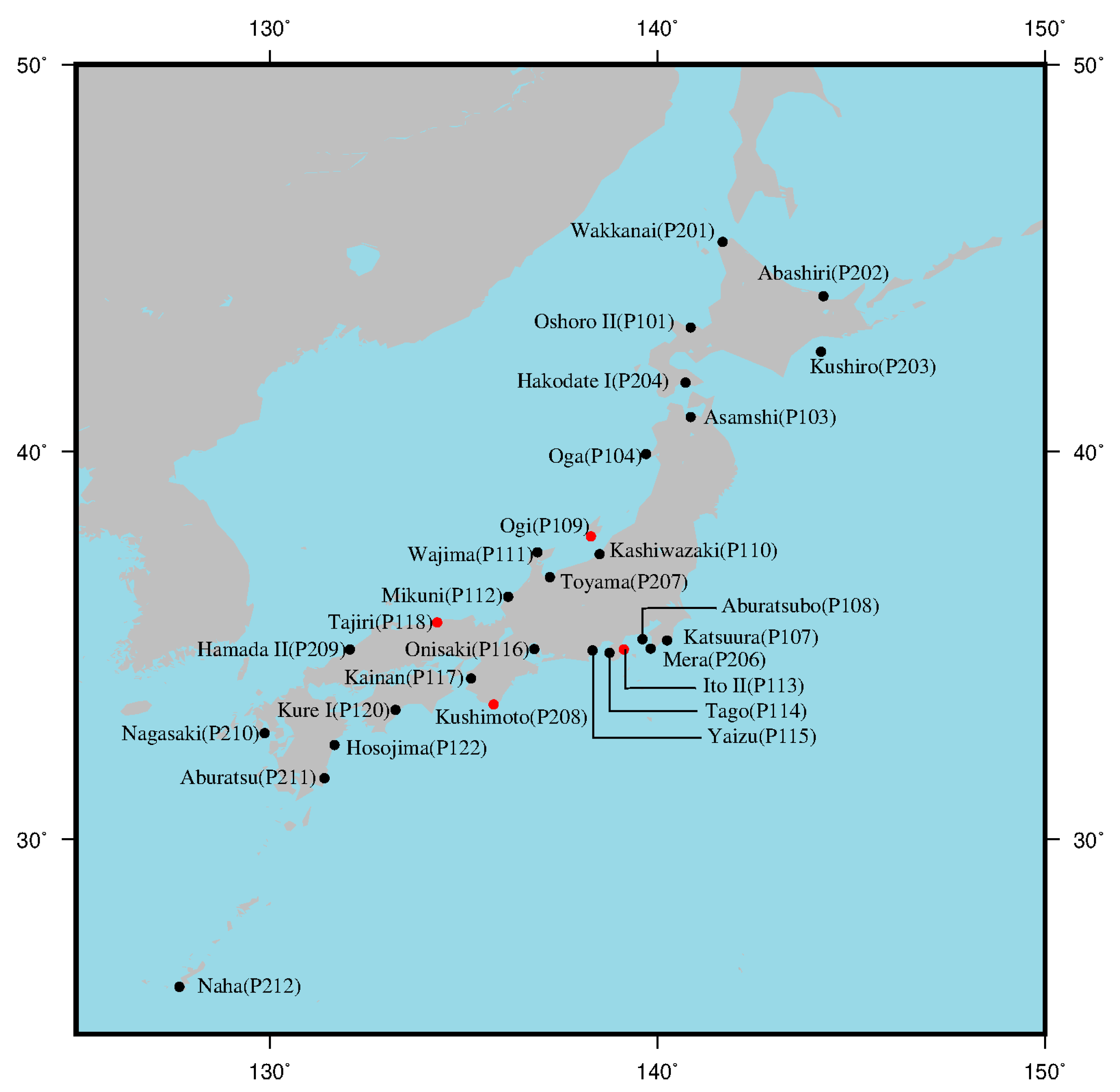
Figure 1. Research area and geographical distribution of tide gauges and joint GNSS stations. Outside of the brackets is the name of tide gauge, and inside the brackets is the name of GNSS station.
Remotesensing 12 04168 g001
Figure 2. The relationship between the sea level measured from the satellite altimeter relative to the reference ellipsoid, the sea level measured from the tide gauges relative to a certain benchmark (revised local reference, RLR), and the height of the benchmark measured from GNSS relative to the reference ellipsoid.
Remotesensing 12 04168 g002
Figure 3. The STDs of the differences of the SSH between SJAO2020A and DTU18, DTU15, Whu13, CLS15 and CLS11 within different distances from the coastline.
Remotesensing 12 04168 g003
Figure 4. SJAO2020 MSS model.
Remotesensing 12 04168 g004
Figure 5. (a) The power spectral density (PSD) of SLA of the along Sentinel-3B tracks using several MSS models, i.e., DTU18 (green), DTU15 (blue), WHU13 (yellow), CLS11 (red), SJAO2020 (black), CLS15 (cyan); (b) The ratio of SLA spectra from panel (a), i.e., PSD (SLA with DTU15)/PSD (SLA with SJAO2020) (mazarine), PSD (SLA with DTU18)/PSD (SLA with SJAO2020) (scarlet), and PSD (SLA with CLS15)/PSD (SLA with SJAO2020) (khaki).
Remotesensing 12 04168 g005
Table 1. Multi-satellite altimeter data used in this study.
SatelliteStart and End DateCyclesSatelliteStart and End DateCycles
TOPEX/ADecember 1992–April 200411–353Envisat/BFebruary 2011–February 2012100–111
Jason-1/AApril 2004–October 200811–249SRLMarch 2013–March 20151–21
Jason-2/AOctober 2008–May 201611–290HY-2AApril 2013–March 201667–117
Jason-3/AMay 2016–December 201811–106Sentinel-3ADecember 2016–January 201912–39
TOPEX/BSeptember 2002–September 2005369–479ERS-1/GMApril 1994–March 199530–40
Jason-1/BFebruary 2009–February 2012262–372Jason-1/GMMay 2012–June 2013500–537
ERS-1/35November 1992–December 1993
March 1995–March 1996
16–27
41–51
CryoSat-2/LRMJanuary 2011–December 201814–113
ERS-2December 1995–December 20037–80SRL/DPJuly 2016–December 2018100–125
GFOMay 2000–May 200845–215HY-2A/GMMarch 2016–January 2019118–230
Envisat/AMay 2002–May 20106–89
Table 2. Corresponding data used for sea level variation corrections of geodetic mission (GM) data.
GM ObservationsCorresponding ERM Data
MissionsCyclesObservation PeriodsMissionsCyclesObservation Periods
ERS-1/GM100–11110 April 1994–21 March 1995T/P57–931 April 1994–3 April 1995
CryoSat-214–11328 January 2011–30 December 2018Jason-294–30320 January 2011–2 October 2016
Jason-31–10617 February 2016–3 January 2019
Jason-1/GM500–5377 May 2012–21 June 2013Jason-2140–18320 April 2012–3 June 2013
HY-2A/GM118–23030 March 2016–4 January 2019Jason-2284–30318 March 2016–2 October 2016
Jason-34–10718 March 2016–13 January 2019
SRL/DP1004 July 2016–31 December 2018Jason-2294–30325 June 2016–2 October 2016
Jason-314–10625 June 2016–2 October 2019
Table 3. Statistical results of crossover differences of sea surface height (SSH) before and after temporal oceanic variability correction.
Altimetric SatelliteBefore Temporal Oceanic Variability Correction (m)After Temporal Oceanic Variability Correction (m)
MeanSTDRMSMeanSTDRMS
TOPEX/A + Jason-1/A + Jason-2/A + Jason-3/A−0.00030.19710.19710.00180.01790.0179
TOPEX/B + Jason-1/B0.01220.15980.1602−0.00230.02910.0292
ERS-1−0.00950.19830.19850.00170.04520.0453
ERS-2−0.00900.22160.2185−0.00490.08150.0816
GFO0.01640.18180.18250.00340.02770.0279
Envisat/A0.01910.18980.1908−0.00240.02580.0260
Envisat/B0.00650.16920.16930.00230.06320.0632
SRL−0.00940.18420.18440.00150.04440.0444
HY-2A0.00120.18670.18670.00050.03280.0328
Sentinel-3A0.00640.18010.1802−0.00300.02930.0295
ERS-1/GM−0.00160.18830.1883−0.00800.12020.1204
Jason-1/GM0.02820.18820.1861−0.00160.11200.1120
Cryosat-2/LRM−0.01890.18660.18760.00020.11090.1109
SRL/DP0.00110.18510.18510.00100.11280.1128
HY-2A/GM0.00160.20210.2021−0.00100.12350.1235
Table 4. The crossover difference after crossover adjustment.
Altimetry SatelliteAfter Crossover Adjustment (m)
MeanSTDRMS
TOPEX/A + Jason-1/A + Jason-2/A + Jason-3/A0.00030.00680.0068
TOPEX/B + Jason-1/B−0.00150.02450.0245
ERS-10.00040.02460.0246
ERS-2−0.00030.04440.0444
GFO0.00080.01550.0155
Envisat/A−0.00020.01590.0159
Envisat/B0.00150.03720.0372
SRL0.00030.02700.0270
HaiYang-2A0.00030.02660.0266
Sentinel-3A0.00030.02570.0257
ERS-1/GM0.00020.09850.0985
Jason-1/GM−0.00070.09420.0942
Cryosat-2/LRM0.00010.09170.0917
SRL/DP0.00040.09510.0951
HY-2A/GM−0.00090.10210.1021
All satellite0.00010.08110.0811
Table 5. Differences between tide gauge stations and MSS models in the coastal area (10 km from the coastline) (units, m).
Tide H t i d e H D T U 18 H C L S 15 H S J A O 2020 A H S J A O 2020 Improvements 1
Ogi38.871838.841038.841038.834838.891745.80%
Tajiri36.625836.245136.190536.679936.639973.94%
Ito II40.506640.429040.448040.394140.470868.17%
Kushimoto39.667639.740739.729839.716039.687459.09%
1 Improvement = 1 | H S J A O 2020 H t i d e | / | H S J A O 2020 A H t i d e | .
Table 6. STD of different MSS models as compared with altimetry data selected on the wavelengths from 35 to 300 km (units, m).
Altimetric SatelliteSJAO2020CLS15DTU18DTU15WHU13CLS11
T/P+Japan-1 + Japan-2 + Japan-3 (31 December 1992–31 December 2018)0.01380.01770.01860.01960.02650.0292
ERS-1 (27 November 1992–30 December 19930.02170.02240.02230.02240.02260.0222
HY-2A (12 April 2014–15 March 2016)0.02010.02200.02220.02280.02550.0264
Sentinel-3B (27 November 2018–5 November 2019)0.02920.03120.03190.03200.03420.0358
SRL (19 March 2015–4 July 2016)0.04350.04210.04430.04490.05170.0529
Jason-2/GM (29 July 2017–14 September 2017)0.04140.04250.04260.04300.04940.0497
Note: The figures for independent datasets (not used in the MSS model) are highlighted in bold.
Publisher’s Note: MDPI stays neutral with regard to jurisdictional claims in published maps and institutional affiliations.