Abstract
Coastal wetlands provide essential ecosystem services and are closely related to human welfare. However, they can experience substantial degradation, especially in regions in which there is intense human activity. To control these increasingly severe problems and to develop corresponding management policies in coastal wetlands, it is critical to accurately map coastal wetlands. Although remote sensing is the most efficient way to monitor coastal wetlands at a regional scale, it traditionally involves a large amount of work, high cost, and low spatial resolution when mapping coastal wetlands at a large scale. In this study, we developed a workflow for rapidly mapping coastal wetlands at a 10 m spatial resolution, based on the recently emergent Google Earth Engine platform, using a machine learning algorithm, open-access Synthetic Aperture Radar (SAR) and optical images from the Sentinel satellites, and two terrain indices. We then generated a coastal wetland map of the Bohai Rim (BRCW10) based on the workflow. It has a producer accuracy of 82.7%, according to validation using 150 wetland samples. The BRCW10 data reflected finer information when compared to wetland maps derived from two sets of global high-spatial-resolution land cover data, due to the fusion of multiple data sources. The study highlights the benefits of simultaneously merging SAR and optical remote sensing images when mapping coastal wetlands.
1. Introduction
Coastal wetlands are the natural transition zone between terrestrial ecosystems and marine ecosystems. They provide many essential ecosystem services, including natural coastal protection, fish nurseries, carbon sequestration, and water quality purification [1,2]. However, coastal wetlands are experiencing substantial changes worldwide due to both anthropogenic activities and natural environmental changes [3,4]. To control the increasingly severe problems and conserve coastal wetlands, it is critical to accurately map coastal wetlands.
The Bohai Rim is the political, economic, and cultural center of northern China. With the rapid social and economic development and climate changes during the past several decades, the area of coastal wetlands in this region has been significantly reduced, and ecosystem service functions have been substantially degraded [5,6,7]. The serious eco-environmental problems, therefore, limit the region’s ability to achieve sustainable development goals. In 2018, three ministries of China enacted an action plan called the tough battle for the comprehensive treatment of the Bohai Sea. Several critical aims of the action plan include implementing strict Bohai ecological protection, stringently controlling reclamation, strengthening coastline and coastal wetlands protection, strengthening the comprehensive renovation and restoration of estuaries and bays, and speeding up solving serious ecological and environmental problems. It is, therefore, critical to develop an easily and rapidly updatable, high spatial resolution, and accurate coastal wetland monitoring workflow to achieve these aims.
Satellite-based remote sensing provides flexible tools to map land characteristics and is widely used to map wetlands at different spatial scales and resolutions [8]. Currently, many remote-sensing-based global and national wetland data are available. Most of these wetland data were derived from optical remote sensing images [9,10]. The spatial resolution of these wetland data is often higher than 200 m. Wetland data with a spatial resolution lower than 100 m have only been available recently [11,12,13]. For example, the National Geomatics Center of China developed a 30 m spatial resolution global land cover product (GlobeLand30), which classified land cover as wetland and nine other types [11]. Gong et al. developed a global 10 m spatial resolution land cover map, which is the first product that provides large scale wetland information at a 10 m spatial resolution [12]. Nevertheless, these data were not specifically designed for deriving accurate coastal wetland maps, and the wetland layers of the data often suffer from low accuracy [12]. Recently, Mao et al. mapped wetland over China at a spatial resolution of 30 m, using the Landsat 8 Operational Land Imager (OLI) images [13]. Wang et al. derived a coastal wetlands map of China at a spatial resolution of 30 m [2], based on the Landsat images and the Google Earth Engine (GEE) platform [14]. Particularly, Bourgeau-Chavez et al. successfully mapped coastal wetlands over the United States and Canadian Laurentian coastal Great Lakes at a high spatial resolution by combining multi-source remote sensing data [15].
Traditionally, accurately mapping wetlands at a large scale and high resolution is an enormous and costly project, because a large number of remote sensing images must be collected and significant image pre-processing work has to be done before the images can be used to derive wetland information. In addition, extensive man-machine interactions are needed in the mapping processes. Coastal wetlands are often fragmented, incomplete, and highly dynamic. Thus, traditional land cover mapping methods cannot always meet the rapidity and accuracy needs for coastal wetlands. The advances in machine learning algorithms, the emergent cloud-computing technologies, and services such as GEE, as well as the recently available, open-access, and high-resolution remote sensing data, make it possible to rapidly monitor coastal wetlands at low cost [16,17].
Many previous studies have demonstrated that complementary information on land targets could be obtained by synthesizing optical and Synthetic Aperture Radar (SAR) remote sensing images [15,18,19,20]. This is largely because SAR sensors are almost unaffected by cloudy and rainy weather, independent of solar radiation and day/night condition, and are more sensitive to the structure, texture, and dielectric characteristics of land targets than optical sensors [21]. Conversely, optical remote sensing is more sensitive to the reflective and spectral characteristics of land targets than SAR images [17]. However, synergistic use of optical and SAR data for wetland mapping is often at small and local scales, due to the limited availability and expensive cost of satellite SAR data. Until recently, the open-access Sentinel-1 SAR data and Sentinel-2 optical data have provided an opportunity for fusing SAR and optical data to monitor wetland at a large scale and high spatial resolution [16,17]. In addition, the location and the extent of wetland are strongly affected by topography. The topographic information is always more stable and reliable than the land surface information derived from optical and SAR data. As for extracting wetland area information, synergistically bringing together topographic information and multi-source remote sensing data outperforms the use of remote sensing data alone [16,18]. The objective of this study was to derive a coastal wetland map of the Bohai Rim at a high spatial resolution, based on the GEE platform and a machine learning algorithm, and by employing the Sentinel-1 SAR images, Sentinel-2 optical images, and topographic information.
2. Materials and Methods
2.1. Study Area
The Bohai Rim is the coastal zone of northern China (Figure 1). It covers the majority of the Beijing–Tianjin–Hebei Region, Liaodong Peninsula, and Shandong Peninsula, and extends to parts of the Shanxi and Inner Mongolia provinces. It is the political, economic, and cultural center of northern China. Coastal wetlands in this region are concentrated and have important ecosystem service functions. In this study, we defined the Bohai Rim coastal region (BRCR) as the Tianjin municipality and the coastal counties around Bohai. It covers an area of approximately 97,157 km2. The land cover types of the BRCR are mainly cropland, forest, impervious land, wetlands, bare land, grasslands, and shrubland (Figure 1). The wetlands are coastal wetlands mainly distributed in the center of the BRCR. The mean annual temperature (MAT) and mean annual precipitation (MAP) of the region are 11.2 ℃ and 614.2 mm/year, respectively. The elevation of the region ranges from 124 m below sea level to 1118 m above sea level.
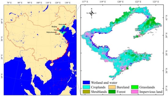
Figure 1.
Location and land cover types of the study area. The land cover data is from the FROM-GLC10 data [12].
2.2. Data Sets and Their Preprocessing
2.2.1. Remote Sensing Data
Following Hird et al. [16], we used the Band2, Band3, Band4, and Band8 data from the Sentinel-2 Level-1C images [22] and the normalized difference vegetation index (NDVI) and the normalized difference water index (NDWI) based on them, three sets of SAR backscatter data from the Sentinel-1 SAR C-band Level-1 Ground Range Detected (GRD) images [23], and two digital elevation model (DEM)-based topographic indexes as the input for the machine learning model (Table 1).

Table 1.
Information in respect of the data sets used in the study.
Both the Sentinel-2 Level-1C and Sentinel-1 SAR C-band Level-1 GRD images (C-band Level-1) during the growing seasons (i.e., May to August) of 2018 and 2019 were accessed and pre-processed through the Google Earth Engine (GEE) platform. The Sentinel-2 Level-1C data pre-processing procedures included cloud-masking, quality controls, mosaic, and median composite. Firstly, low noise and cloud images were filtered out according to a quality flag band and a threshold of Band1. Then, the NDVI and NDWI were calculated as NDVI = (Band8 − Band4)/(Band8 + Band4), and NDWI = (Band8 − Band3)/(Band8 + Band3). The values of NDVI and NDWI in the BRCR ranged from −0.69 to 0.96 and from −0.87 to 0.75, respectively (Figure 2). The spectral values of the bands were between 20 and 22,764.
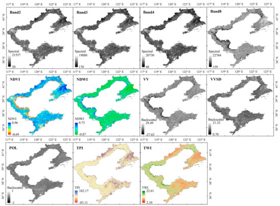
Figure 2.
Spatial distributions of the input variables.
The Sentinel-1 SAR data used included the C-band vertical–vertical polarization (VV) backscatter data and its standard deviation (VVSD), and a normalized polarization (POL) index, which was calculated based on the VV and vertical–horizontal polarization (VH) images, POL = (VH − VV)/(VH + VV). Both ascending and descending orbits, with the interferometric wide swath model and average incidence angles between 30 and 40° were collected in this study. The pre-processes included thermal noise removal, radiometric calibration, and terrain correction. As shown in Figure 2, the VV backscatter values ranged from −27.6 to 29.5 dB. The standard deviation of VV backscatter data (VVSD) ranged from 0.7 to 21.3 dB. The range of POL was between −1 and 1.
2.2.2. Topographic Data
The DEM-based topographic wetness index (TWI) [24] and topographic position index (TPI) [25] were used to represent the topographic information in this study. The DEM data were from the Advanced Spaceborne Thermal Emission and Reflection Radiometer (ASTER) Global Digital Elevation Model version 2 (GDEM v2), which is a global open-access DEM at 30 m spatial resolution. To match with the remote sensing data, the ASTER GDEM v2 was re-gridded to a 10 m spatial resolution before it was used in calculating TWI and TPI. TPI represents the elevational position of each pixel relative to the average elevation of its neighboring pixels. It reflects local topographic position and can be used to indicate low-lying areas, which are general wetlands. It is calculated as
where i is the elevation of pixel or cell i, and is the average elevation of all the pixels within a given radius, r. Following Hird et al. [16], we used a radius value of 100 m. TWI indicates the potential soil water storage condition of a pixel. It is calculated as
where SCA is the special catchment area, and is the slope angle. In this study, we used the open geographic information system (GIS) software System for Automated Geoscientific Analyses (SAGA) [26] to calculate TPI and TWI. The TPI and TWI ranged from −83.1 to 102.2 and from 2.1 to 22.6, respectively (Figure 2).
2.2.3. Samples and Evaluation Data
The training samples of machine learning models were obtained by identifying 8000 random points in the BRCR, based on Google Earth, Landsat images, and field surveys (Figure S1). The input values of the training samples were acquired using the ArcGIS tool of Extract Multi Values to Points. The validating data included 150 wetland samples, which were derived from published literature and field surveys (Figure S1).
We also compared our produced wetland map of the Bohai Rim to that derived from the GlobeLand30 [11] and FROM-GLC10 [12] data (Table 1). GlobeLand30 data was derived from Landsat Thematic Mapper/Enhanced Thematic Mapper Plus (TM/ETM+) and Chinese HJ-1 images that were acquired during 2009–2011, with a spatial resolution of 30 m. The FROM-GLC10 data were derived from Sentinel-2 images that were accessed during 2017 and has a spatial resolution of 10 m. We used the wetland maps derived from these land cover data by extracting the water body and wetland classes.
2.2.4. Method
Random forest (RF) was used to train and predict the coastal wetlands of the Bohai Rim in this study. It is a machine learning algorithm that employs an ensemble of regression or classification trees to assign a value or class to a response variable [27]. The RF model has several advantages in remote sensing classification, including running efficiently on large data; no need for variable deletion; giving variables importance in terms of node purity (i.e., the Gini index); generating generalization error (i.e., out-of-bag (OOB) error); and is robust to outliers and noise [15,28,29]. We used the randomForest package [30] in R software (version 3.5.2, R Core Team, 2018) to run our RF models. A 10-fold cross validation was used to evaluate the performance of the RF models. Four fifths of the 8000 samples were used for training and the remaining fifth were used for internal validation for each simulation. The two key parameters of the RF model are the number of trees (ntree) and the number of variables considered at each node within a tree (mtry). We decided the ntree and mtry values by first gradually testing mtry values from 1 to 6 and choosing the optimal mtry, and then using the optimal mtry and the variety in model internal error to select ntree. When modeling the coastal wetlands of the whole BRCR, we tested different combinations of the fixed ntree and variable mtry and chose the best models according to the OOB errors. We also used the Gini index to compare the importance of the 11 input variables for predicting coastal wetlands. The Gini index (i.e., MeanDecreaseGini) is a measure of variable importance for predicting a target variable. A higher MeanDecreaseGini indicates higher variable importance.
The workflow includes three steps (Figure 3). The first step is data pre-processing. Eleven input variables were collected and pre-processed. The TPI and TWI were derived from DEM using the SAGA software [26]. Both the Sentinel-1 SAR images and the Sentinel-2 optical images were pre-processed on the GEE platform. The second step is sample preparation and RF model training. We obtained training samples by randomly generating 8000 random points in the study area and extracting values of the 11 input variables corresponding to the random points, using ArcGIS software (version 10.5, ESRI, 2016). The random points were then artificially identified as to whether they were wetlands through Google Earth, Landsat 8 images, and field surveys. To determine which combination of the input variables had the best performance for predicting coastal wetlands, we selected a small sub-region called Beidagang (Figure S2) in the study area and designed four RF model experiments, because of the large computational cost in running the RF models across the whole BRCR. The four experiments included optical remote sensing inputs (i.e., Band2, Band3, Band4, Band8, NDVI, and NDWI) (Omodel); SAR remote sensing inputs (VV, VVSD, and POL) (Smodel); optical and SAR inputs (Band2, Band3, Band4, Band8, NDVI, NDWI, VV, VVSD, and POL) (OSmodel), and optical, SAR, and topographic inputs (Band2, Band3, Band4, Band8, NDVI, NDWI, VV, VVSD, POL, TPI, and TWI) (OSTmodel). The optimum RF model was selected according to the OOB errors and 10-fold cross-validations of the models. Finally, the final coastal wetland is predicted using the 11 input variables and the optimum RF model, and is validated using the independent wetland samples from published literature and field surveys by calculating the producer accuracy.
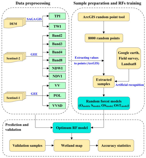
Figure 3.
The workflow of the proposed coastal wetland mapping.
3. Results
3.1. Mapping Coastal Wetlands Using Random Forests and Different Input Variables
We chose a small wetland in the BRCR named Beidagang (Figure S2) to run the model experiments and to determine the best combination of the input variables. As shown in Figure 4, each of the RF models could identify the main contours of the Beidagang wetland, while significant differences existed between different models. According to the high-resolution ArcGIS image (Figure S2) and field survey, although the Omodel (Figure 4a) derived the main extent of the wetland, it failed to identify the wetlands in the western Beidagang. The percentage of wetland pixels based on the Omodel was 33.5%, which was significantly lower than that based on the other RF models. The Smodel (Figure 4b) clearly recognized water bodies and wet regions with a wetland percentage of 35.4%, while it did not identify many non-vegetated areas and small wetlands around these areas. The OSmodel (Figure 4c) and OSTmodel (Figure 4d) showed a similar wetland map and reflected the wetland extent with more details when compared to that of the Omodel and Smodel (Figure 4a, b). The OSmodel suggested that wetland, vegetated land, and non-vegetated land accounted for 36.2, 43.6, and 20.2%, respectively, of the total area. The OSTmodel indicated that the percentages of wetland, vegetated land, and non-vegetated land were 35.1, 42.5, and 22.4%, respectively. The 10-fold cross-validation accuracies of the Omodel, Smodel, OSmodel, and OSTmodel were 95.8, 96.2, 97.0, and 97.1%, respectively (Table 2). The OSTmodel showed the lowest OOB error, with a value of 2.91%, followed by the OSmodel, Smodel, and Omodel, with values of 3.0, 3.8, and 4.0%, respectively. Consequently, the OSTmodel was utilized to predict the coastal wetlands over the BRCR.
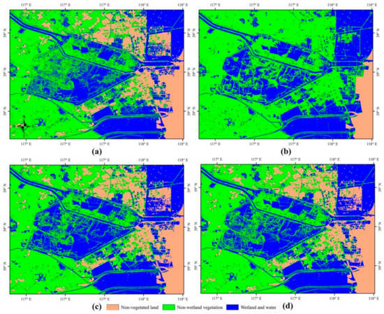
Figure 4.
Coastal wetland maps of the Beidagang predicted by different random forest models: (a) Omodel, (b) Smodel, (c) OSmodel, and (d) OSTmodel.
Table 2.
Parameters and error statistics of the random forest models.
3.2. The High Spatial Resolution Coastal Wetland Data of the Bohai Rim
We generated a coastal wetland map of Bohai Rim at 10 m spatial resolution (BRCW10), using the OSTmodel model. It clearly showed that coastal wetlands of the BRCR are mainly distributed in the Bohai Bay and Laizhou Bay (Figure 5). Coastal wetlands covered almost all the coastal regions of the Bohai Bay, western Laizhou Bay, and southern Laizhou Bay, while along the coastline in the Liaodong Bay, Liaodong Peninsula, and Shandong Peninsula, there were only small and scattered coastal wetlands. The spatial characteristics of coastal wetlands in the three main river estuaries in the Bohai Rim were significantly different. In the Liaohe estuary, wetlands were mainly distributed along the rivers and coastline. In this region, the wetlands were less affected by human activities, and the vegetation cover was high. The coastal wetlands in the Haihe estuary were concentrated in several regions along the rivers and coastline. They were largely impacted by human activities, which meant many wetlands have been reclaimed or converted to impervious lands during the past several decades [6,31,32]. The distributions of coastal wetlands in the Yellow River estuary were wider than that of the Liaohe estuary and Haiihe estuary. The coastal wetlands were continuously distributed along the coastline, and suffered from serious reclamation [3,33]. Based on our produced BRCW10 data, the coastal wetlands, non-wetland vegetation, and non-vegetation land occupied 8.1, 83.1, and 8.8% of the BRCR, respectively.
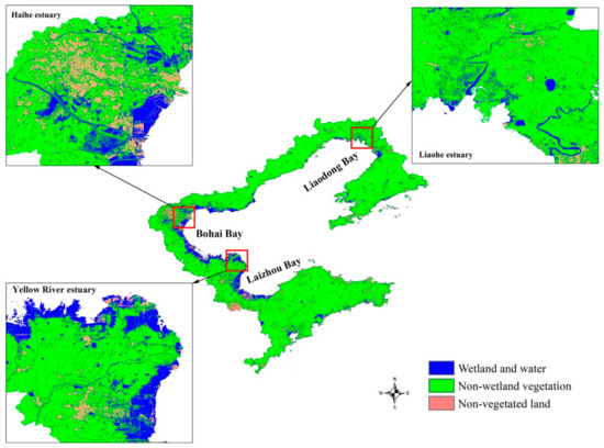
Figure 5.
The Bohai Rim coastal wetland map predicted by the OSTmodel model.
3.3. Performance and Evaluation of the Coastal Wetland Map
The 10-fold cross-validation accuracy of the BRCW10 data is 97.0%, which is the same as the accuracy of the OSTmodel model experiment (Table 2). Based on the independent 150 wetland samples from the published literature and field surveys (Figure 1), we found that BRCW10 has a producer accuracy of 82.7%. The patterns of BRCW10 were similar to the wetland map derived from the FROM-GLC10 data (Figure 6). The GlobeLand30-based wetland map showed a similar spatial distribution to that of the BRCW10 and FROM-GLC10 in the Bohai Bay and Laizhou Bay, while it had a much larger wetland extent in the Liaohe estuary (Figure 7). Compared to FROM-GLC10, BRCW10 identified finer coastal wetlands information in the Haihe river estuary. For example, it successfully recognized the Beidagang wetland, which was not well identified by the FROM-GLC10. The GlobeLand30 map showed more continuous wetlands and non-vegetation lands than that of the BRCW10 and the FROM-GLC10. The patterns of the coastal wetlands in the Yellow River estuary from the three data sets were similar overall. The BRCW10 data showed more detailed information on the wetlands than that of FROM-GLC10 and GlobeLand30. In the Liaohe estuary, the spatial distributions of the coastal wetlands were significantly different between the three data sets. The GlobeLand30 showed a much larger and continuous wetland extent than that of BRCW10 and FROM-GLC10. Consistent with the situation in the Haihe estuary, the BRCW10 data recognized more wetlands than those of the FROM-GLC10 in the Liaohe estuary. The statistics suggested that the area of coastal wetlands based on the BRCW10 data was 8095.8 km2, which was much larger than that based on the FROM-GLC10 data (6560.6 km2) but less than that using the GlobeLand30 data (8660.4 km2) (Table S1). The percentage of wetland pixels of GlobeLand30 (9.0%) was largest, followed by BRCW10 (8.1%) and FROM-GLC10 (6.5%).
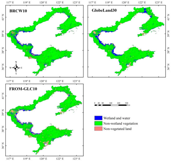
Figure 6.
Comparisons among BRCW10, GlobeLand30, and FROM-GLC10 wetland maps.
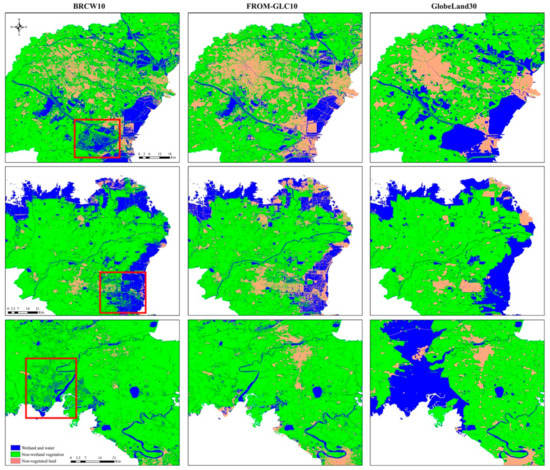
Figure 7.
Comparisons of the BRCW10 and corresponding coastal wetlands maps derived from the FROM-GLC10 and the GlobeLand30 data at the Haihe estuary (top row), Yellow River estuary (middle row), and Liaohe estuary (bottom row). The red boxes delineate examples of regions with large differences among the data sets.
4. Discussion
4.1. The Importance of the Input Variables
We synergistically used 11 variables based on optical and SAR remote sensing images, and DEM-based topographic data, to derive coastal wetland information for the BRCR. Many previous studies have demonstrated the importance of simultaneously using optical and SAR remote sensing data when mapping wetlands [15,16,18,19,20,34,35]. In this study, the variable importance based on the Gini index confirmed these studies. The mean decrease in the Gini index of the RF models indicated that the most important variables in the Omodel, Smodel, OSmodel, and OSTmodel were, respectively, NDWI, VV, VV, and VV (Figure 8). The three most important variables of the Omodel were NDWI, NDVI, and Band8. Band4, Band3, and Band2 showed comparable but relatively small importance. In the Smodel, the importance of VV was much larger than that of POL and VVSD. The importance of the variables decreased gradually in the OSmodel with the highest rankings of the variables from VV, NDWI, NDVI, and Band8 to POL. However, VVSD, Band4, Band2, and Band3 showed much smaller importance. In the optimum OSTmodel, the six most important variables were VV, NDWI, NDVI, Band8, POL, and TWI. The other five variables (i.e., VVSD, Band4, Band3, Band2, and TPI) showed small and nearly identical importance. These results suggest that a more effective RF model can be obtained by coupling SAR images, optical images, and topography data together as inputs.
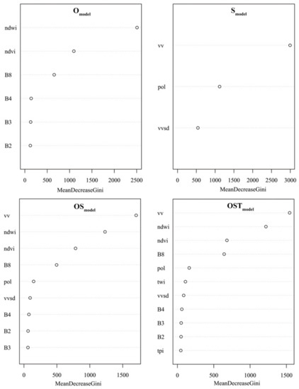
Figure 8.
Input variable importance according to the Gini index of the random forest models including Omodel, Smodel, OSmodel, and OSTmodel.
4.2. Differences between BRCW10 and Land Cover Data Derived Coastal Wetland Maps
We compared the BRCW10 to two coastal wetland maps derived from the FROM-GLC10 and GlobeLand30 land cover products. The results suggested that patterns of the three wetland maps were similar (Figure 6), however, there were also significant differences between them. The GlobeLand30 map showed more continuous wetlands and non-vegetation lands than those of BRCW10 and FROM-GLC10. An important reason is that a minimum size post-processing procedure was applied for the classification [11]. Especially in the Liaohe estuary, the GlobeLand30 wetland map showed a much larger and continuous wetland extent than those of BRCW10 and FROM-GLC10 (Figure 7). This is probably due to the information from auxiliary data, including the China land cover map [31] and Global Lakes and Wetlands Database [9] that were merged into the GlobeLand30 data. The definition and extent of wetlands in the auxiliary data might not be identical with those directly derived from remote sensing data. Consequently, our statistics suggested that the total area of coastal wetlands based on the GlobeLand30 data was significantly larger than that of the BRCW10 and FROM-GLC10 data. Besides the differences in the classification methods, the differences in the coastal wetlands from the three data sets may also be partially attributed to the different periods of the data (Table S1).
The differences between the BRCW10 wetland map and the two land cover data derived wetland maps were further analyzed by comparing the corresponding differences in the three most important input variables (i.e., NDVI, NDWI, and VV). The pixels that were wetland in the BRCW10 map but not in the FROM-GLC10 or the GlobLand30 maps were mainly distributed in several small regions in the Bohai Bay and Laizhou Bay (Figure 9). The corresponding NDVI and NDWI were mainly less than 0.4 and 0.5, respectively, suggesting that BRCW10 identified more bare land and low vegetation pixels as wetland than FROM-GLC10 and GlobLand30. The corresponding VV pixels were mainly < −5 dB, indicating that BRCW10 classified more wet pixels into wetland class. The NDVI and NDWI pixels that were wetland in FROM-GLC10 and GlobLand30 but not in BRCW10 were mainly positive and negative, respectively (Figure 10). The corresponding VV pixels ranged from −20 to 0 dB. These results suggested that FROM-GLC10 and GlobLand30 classified some wet vegetated pixels and bare land pixels into the wetland class that were not wetland in the BRCW10 data. However, the number of pixels that were wetland in FROM-GLC10 and GlobLand30 but not in BRCW10 were much smaller than the number of pixels that were wetland in BRCW10 but not in FROM-GLC10 and GlobLand30. The analyses demonstrated the benefits of simultaneously merging SAR and optical remote sensing images when mapping coastal wetlands.
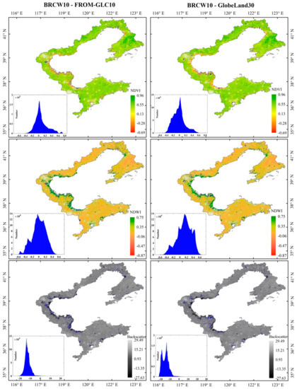
Figure 9.
Spatial and frequency distributions of the normalized difference vegetation index (NDVI), normalized difference water index (NDWI), and vertical–vertical polarization (VV) pixels that were wetland in the BRCW10 wetland map but not in the FROM-GLC10 (left column) and in the GlobLand30 (right column) derived wetland maps.
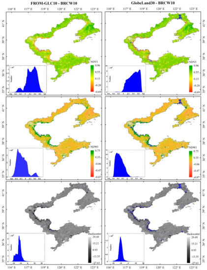
Figure 10.
Spatial and frequency distributions of the NDVI, NDWI, and VV pixels that were wetland in the FROM-GLC10 (left column) and in the GlobLand30 wetland maps (right column) but not in the BRCW10 wetland data.
5. Conclusions
We developed a workflow for rapidly mapping coastal wetlands, based on the GEE platform and using the random forest model, open-access and multi-remote sensing data, and topographic information. Based on the workflow, a coastal wetland map of the Bohai Rim at a spatial resolution of 10 m was derived. The coastal wetland map has a producer accuracy of 82.7%, according to validation using 150 wetland samples from published literature and field surveys. The study demonstrated the possibility of rapidly monitoring land characteristics using the GEE platform, machine learning algorithms, and current open-access and high-resolution satellite data. It also highlighted the importance of simultaneously merging SAR and optical remote sensing images when mapping coastal wetlands. The coastal wetland data provides fundamental coastal wetland information over the BRCR at a high spatial resolution. Such information is critical for coastal wetland resource management, policy development, and research. The workflow in this study is also valuable for rapidly monitoring other land cover characteristics with GEE, machine learning algorithms, and open-access and high-resolution satellite data. We defined coastal wetlands including both water bodies and wetlands and did not divide wetlands into sub-classes. Future study should focus on mapping the coastal wetlands using a standard classification system. The BRCW10 data and auxiliary data including BRCR-NDVI and BRCR-NDWI are available from https://doi.org/10.6084/m9.figshare.12792626.
Supplementary Materials
The following are available online at https://www.mdpi.com/2072-4292/12/24/4114/s1, Figure S1: Spatial distributions of the training samples and validation samples; Table S1: Statistics of the area of the Bohai rim coastal wetlands based on different data sets.
Author Contributions
Conceptualization, S.S. and Y.Z. (Yonggen Zhang); methodology, S.S.; software, S.S.; validation, C.C., X.R., and Y.W.; formal analysis, S.S., W.C.; investigation, S.S.; resources, Z.S.; data curation, S.S.; writing—original draft preparation, S.S.; writing—review and editing, Z.S., B.C., Y.Z. (Yangjian Zhang), and W.Y.; visualization, S.S. All authors have read and agreed to the published version of the manuscript.
Funding
The research was supported by the Natural Science Foundation of Tianjin City (20JCQNJC01560), the National Natural Science Foundation of China (41801061, 41930862), and the Peiyang Young Scholar Program of Tianjin University (2020XRG-0066).
Acknowledgments
The authors thank Jen Hird for her contributions on the choice and preparation of the model inputs, and Su Ding for her help on the RF model.
Conflicts of Interest
The authors declare no conflict of interest.
References
- Schuerch, M.; Spencer, T.; Temmerman, S.; Kirwan, M.L.; Wolff, C.; Lincke, D.; McOwen, C.J.; Pickering, M.D.; Reef, R.; Vafeidis, A.T.; et al. Future response of global coastal wetlands to sea-level rise. Nature 2018, 561, 231–234. [Google Scholar] [CrossRef]
- Wang, X.; Xiao, X.; Zou, Z.; Hou, L.; Qin, Y.; Dong, J.; Doughty, R.B.; Chen, B.; Zhang, X.; Chen, Y.; et al. Mapping coastal wetlands of China using time series Landsat images in 2018 and Google Earth Engine. ISPRS J. Photogramm. Remote Sens. 2020, 163, 312–326. [Google Scholar] [CrossRef]
- Cui, B.; He, Q.; Gu, B.; Bai, J.; Liu, X. China’s coastal wetlands: Understanding environmental changes and human impacts for management and conservation. Wetlands 2016, 36, 1–9. [Google Scholar] [CrossRef]
- Martín-Antón, M.; Negro, V.; del Campo, J.M.; López-Gutiérrez, J.S.; Esteban, M.D. Review of coastal land reclamation situation in the world. J. Coastal Res. 2016, 75, 667–671. [Google Scholar] [CrossRef]
- Wu, W.; Tian, B.; Zhou, Y.; Shu, M.; Qi, X. The trends of coastal reclamation in China in the past three decades. Acta Ecol. Sin. 2016, 36, 5007–5016. (In Chinese) [Google Scholar] [CrossRef]
- Ding, X.; Shan, X.; Chen, Y.; Jin, X.; Muhammed, F.R. Dynamics of shoreline and land reclamation from 1985 to 2015 in the Bohai Sea, China. J. Geogr. Sci. 2020, 29, 2031–2046. [Google Scholar] [CrossRef]
- Liu, Y.; Li, J. The patterns and driving mechanisms of reclaimed land use in China’s coastal areas in recent 30 years. Sci. Sin. 2020, 50, 761–774. (In Chinese) [Google Scholar] [CrossRef]
- Gabrielsen, C.G.; Murphy, M.A.; Evans, J.S. Using a multiscale, probabilistic approach to identify spatial-temporal wetland gradients. Remote Sens. Environ. 2016, 184, 522–538. [Google Scholar] [CrossRef]
- Lehner, B.; Döll, P. Development and validation of a global database of lakes, reservoirs and wetlands. J. Hydrol. 2004, 296, 1–22. [Google Scholar] [CrossRef]
- Niu, Z.; Zhang, H.; Wang, X.; Yao, W.; Zhou, D.; Zhao, K.; Zhao, H.; Li, N.; Huang, H.; Li, C.; et al. Mapping wetland changes in China between 1978 and 2008. Chin. Sci. Bull. 2012, 57, 2813–2823. [Google Scholar] [CrossRef]
- Chen, J.; Cao, X.; Peng, S.; Ren, H. Analysis and applications of GlobeLand30: A review. ISPRS Int. J. Geo-Inf. 2017, 6, 230. [Google Scholar] [CrossRef]
- Gong, P.; Liu, H.; Zhang, M.; Li, C.; Wang, J.; Huang, H.; Clinton, N.; Ji, L.; Li, W.; Bai, Y.; et al. Stable classification with limited sample: Transferring a 30-m resolution sample set collected in 2015 to mapping 10-m resolution global land cover in 2017. Sci. Bull. 2019, 64, 370–373. [Google Scholar] [CrossRef]
- Mao, D.; Wang, Z.; Du, B.; Li, L.; Tian, Y.; Jia, M.; Zeng, Y.; Song, K.; Jiang, M.; Wang, Y. National wetland mapping in China: A new product resulting from object-based and hierarchical classification of Landsat 8 OLI images. ISPRS J. Photogramm. Remote Sens. 2020, 164, 11–25. [Google Scholar] [CrossRef]
- Gorelick, N.; Hancher, M.; Dixon, M.; Ilyushchenko, S.; Thau, D.; Moore, R. Google Earth Engine: Planetary-scale geospatial analysis for everyone. Remote Sens. Environ. 2017, 202, 18–27. [Google Scholar] [CrossRef]
- Bourgeau-Chavez, L.; Endres, S.; Battaglia, M.; Miller, M.; Banda, E.; Laubach, Z.; Higman, P.; Chow-Fraser, P.; Marcaccio, J. Development of a bi-national Great Lakes coastal wetland and land use map using three-season PALSAR and Landsat imagery. Remote Sens. 2015, 7, 8655–8682. [Google Scholar] [CrossRef]
- Hird, J.; DeLancey, E.; McDermid, G.; Kariyeva, J. Google Earth Engine, open-access satellite data, and machine learning in support of large-area probabilistic wetland mapping. Remote Sens. 2017, 9, 1315. [Google Scholar] [CrossRef]
- Mahdianpari, M.; Salehi, B.; Mohammadimanesh, F.; Homayouni, S.; Gill, E. The first wetland inventory map of Newfoundland at a spatial resolution of 10 m using Sentinel-1 and Sentinel-2 data on the Google Earth Engine cloud computing platform. Remote Sens. 2018, 11, 43. [Google Scholar] [CrossRef]
- Bwangoy, J.-R.B.; Hansen, M.C.; Roy, D.P.; Grandi, G.D.; Justice, C.O. Wetland mapping in the Congo Basin using optical and radar remotely sensed data and derived topographical indices. Remote Sens. Environ. 2010, 114, 73–86. [Google Scholar] [CrossRef]
- van Beijma, S.; Comber, A.; Lamb, A. Random forest classification of salt marsh vegetation habitats using quad-polarimetric airborne SAR, elevation and optical RS data. Remote Sens. Environ. 2014, 149, 118–129. [Google Scholar] [CrossRef]
- Niculescu, S.; Boissonnat, J.-B.; Lardeux, C.; Roberts, D.; Hanganu, J.; Billey, A.; Constantinescu, A.; Doroftei, M. Synergy of high-resolution radar and optical images satellite for identification and mapping of wetland macrophytes on the Danube Delta. Remote Sens. 2020, 12, 2188. [Google Scholar] [CrossRef]
- Adeli, S.; Salehi, B.; Mahdianpari, M.; Quackenbush, L.J.; Brisco, B.; Tamiminia, H.; Shaw, S. Wetland monitoring using SAR data: A meta-analysis and comprehensive review. Remote Sens. 2020, 12, 2190. [Google Scholar] [CrossRef]
- Drusch, M.; Del Bello, U.; Carlier, S.; Colin, O.; Fernandez, V.; Gascon, F.; Hoersch, B.; Isola, C.; Laberinti, P.; Martimort, P.; et al. Sentinel-2: ESA’s optical high-resolution mission for GMES operational services. Remote Sens. Environ. 2012, 120, 25–36. [Google Scholar] [CrossRef]
- Torres, R.; Snoeij, P.; Geudtner, D.; Bibby, D.; Davidson, M.; Attema, E.; Potin, P.; Rommen, B.; Floury, N.; Brown, M.; et al. GMES Sentinel-1 mission. Remote Sens. Environ. 2012, 120, 9–24. [Google Scholar] [CrossRef]
- Wilson, J.P.; Gallant, J.C. Primary topographic attributes. In Terrain Analysis: Principles and Applications; Wilson, J.P., Gallant, J.C., Eds.; John Wiley & Sons: Hoboken, NJ, USA, 2000. [Google Scholar] [CrossRef]
- Beven, K.J.; Kirkby, M.J. A physically based, variable contributing area model of basin hydrology. Hydrol. Sci. Bull. 1979, 24, 43–69. [Google Scholar] [CrossRef]
- Conrad, O.; Bechtel, B.; Bock, M.; Dietrich, H.; Fischer, E.; Gerlitz, L.; Wehberg, J.; Wichmann, V.; Böhner, J. System for Automated Geoscientific Analyses (SAGA) v. 2.1.4. Geosci. Model Dev. 2015, 8, 1991–2007. [Google Scholar] [CrossRef]
- Breiman, L. Random Forests. Mach. Learn. 2001, 45, 5–32. [Google Scholar] [CrossRef]
- Gislason, P.O.; Benediktsson, J.A.; Sveinsson, J.R. Random Forests for land cover classification. Pattern Recognit. Lett. 2006, 27, 294–300. [Google Scholar] [CrossRef]
- Rodriguez-Galiano, V.F.; Ghimire, B.; Rogan, J.; Chica-Olmo, M.; Rigol-Sanchez, J.P. An assessment of the effectiveness of a random forest classifier for land-cover classification. ISPRS J. Photogramm. Remote Sens. 2012, 67, 93–104. [Google Scholar] [CrossRef]
- Breiman, L.; Cutler, A. Breiman and Cutler’s Random Forests for Classification and Regression. CRAN Package ‘randomForest’ Version 4.6-14. 2018. Available online: https://cran.r-project.org/web/packages/randomForest/ (accessed on 16 December 2020).
- Liu, J.; Zhang, Z.; Xu, X.; Kuang, W.; Zhou, W.; Zhang, S.; Li, R.; Yan, C.; Yu, D.; Wu, S.; et al. Spatial patterns and driving forces of land use change in China during the early 21st century. J. Geogr. Sci. 2010, 20, 483–494. [Google Scholar] [CrossRef]
- Zhang, D.; Sun, S.; Song, Z.; Measho, S. Vegetation dynamics and their drivers in the Haihe river basin, Northern China, 1982–2012. Geocarto Int. 2020, 1–17. [Google Scholar] [CrossRef]
- Liu, Y.; Hou, X.; Li, X.; Song, B.; Wang, C. Assessing and predicting changes in ecosystem service values based on land use/cover change in the Bohai Rim coastal zone. Ecol. Indic. 2020, 111, 106004. [Google Scholar] [CrossRef]
- Corcoran, J.; Knight, J.; Brisco, B.; Kaya, S.; Cull, A.; Murnaghan, K. The integration of optical, topographic, and radar data for wetland mapping in northern Minnesota. Can. J. Remote Sens. 2014, 37, 564–582. [Google Scholar] [CrossRef]
- Merchant, M.A.; Warren, R.K.; Edwards, R.; Kenyon, J.K. An Object-Based Assessment of Multi-Wavelength SAR, Optical Imagery and Topographical Datasets for Operational Wetland Mapping in Boreal Yukon, Canada. Can. J. Remote Sens. 2019, 45, 308–332. [Google Scholar] [CrossRef]
Publisher’s Note: MDPI stays neutral with regard to jurisdictional claims in published maps and institutional affiliations. |
© 2020 by the authors. Licensee MDPI, Basel, Switzerland. This article is an open access article distributed under the terms and conditions of the Creative Commons Attribution (CC BY) license (http://creativecommons.org/licenses/by/4.0/).