Article

Surface Energy Flux Estimation in Two Boreal Settings in Alaska Using a Thermal-Based Remote Sensing Model

1
Geophysical Institute, University of Alaska Fairbanks, Fairbanks, AK 99775, USA
2
Hydrology and Remote Sensing Laboratory, United States Department of Agriculture, Agriculture Research Service, Beltsville, MD 20705, USA
3
Alaska Satellite Facility, Geophysical Institute, University of Alaska Fairbanks, Fairbanks, AK 99775, USA
*
Author to whom correspondence should be addressed.
Remote Sens. 2020, 12(24), 4108; https://doi.org/10.3390/rs12244108
Submission received: 6 November 2020 / Revised: 13 December 2020 / Accepted: 14 December 2020 / Published: 16 December 2020
(This article belongs to the Section Environmental Remote Sensing)

Abstract

:
Recent Arctic warming has led to changes in the hydrological cycle. Circum-Arctic and circumboreal ecosystems are showing evidence of “greening” and “browning” due to temperature warming leading to shrub encroachment, tree mortality and deciduousness. Increases in latent heat flux from increased evapotranspiration rates associated with deciduous-dominated ecosystems may be significant, because deciduous vegetation has extremely high-water use and water storage capacity compared to coniferous and herbaceous plant species. Thus, the impact of vegetation change in boreal ecosystems on regional surface energy balance is a significant knowledge gap that must be addressed to better understand observed trends in water use/availability and tree mortality. To this end, output from a two-source energy balance model (TSEB) with modifications for high latitude boreal ecosystems was evaluated using flux tower measurements and Terra/Aqua MODIS remote sensing data collected over the two largest boreal forest types in Alaska (birch and black spruce). Data under clear and overcast days and from leaf-out to senescence from 2012 to 2016 were used for validation. Using flux tower observations and local model inputs, modifications to the model formulation for soil heat flux, net radiation partitioning, and canopy transpiration were required for the boreal forest. These improvements resulted in a mean absolute percent difference of around 23% for turbulent daytime fluxes when surface temperature from the flux towers was used, similar to errors reported in other studies conducted in warmer climates. Results when surface temperature from Terra/Aqua MODIS estimates were used as model input suggested that these model improvements are pertinent for regional scale applications. Vegetation indices and LAI time-series from the Terra/Aqua MODIS products were confirmed to be appropriate for energy flux estimation in the boreal forest to describe vegetation properties (LAI and green fraction) when field observations are not available. Model improvements for boreal settings identified in this study will be implemented operationally over North America to map surface energy fluxes at regional scales using long time series of remote sensing estimates as part of NOAA’s GOES Evapotranspiration and Drought Information System.

Graphical Abstract

1. Introduction

In the recent past, a significant increase in air temperature in the Arctic [1], also known as the Arctic amplification, is leading to an accelerated increase in air temperatures compared to other parts of the globe inducing broad sea-ice retreat, snow and ice melting and increases in sea level [2,3]. Arctic and sub-Arctic ecosystems in Alaska, dominated by tundra and boreal forest land covers, are witnessing singular changes due to climate warming including widespread permafrost degradation, increases in the area burned and the severity of wildfires, decreased thickness and duration of winter snow cover, acceleration of the hydrological cycle and, rises in river discharge and important vegetation changes in both structure and distribution [4,5,6,7,8,9,10,11]. Furthermore, land surface Arctic hydrologic feedbacks to changing climate are actively coupled to the energy balance of these ecosystems [12]; and in turn, the partitioning of this energy balance plays a critical role in the hydrologic cycle regulation [13].
Circum-Arctic and circumboreal ecosystems are showing evidence of “greening” and “browning” [14,15,16,17], respectively, especially in Alaska and Western Canada. Due to increased temperatures there has been a rise in deciduous shrubs in the Circum-Arctic, which is responsible for the “greening” of the Arctic tundra [16,18] resulting in nearly a 14% increase in vegetation cover [4]. On the other hand, some boreal forest regions are showing “browning” caused by higher coniferous tree mortality because of warmer and drier conditions. Moreover, a higher frequency and intensity of wildfires is changing the boreal forest composition, increasing deciduous tree and shrub cover composition due to their higher drought tolerance and their ability to establish quickly after disturbance [15,19,20,21]. Hence, the transition zone between forest and tundra ecosystems in the northern boundary is expanding both latitudinally and in elevation and is leading to an increase of tree heights and shrub growth leading to denser and taller canopies [16,22].
The impact of vegetation change in boreal ecosystems on the regional surface energy balance is a significant knowledge gap that must be addressed. Filling this knowledge gap is critical for quantifying feedbacks to, and responses and vulnerability of, this landscape to continued climate warming, shifts in hydrology, and increased disturbance from wildfires [13,23]. Increases in latent heat flux associated with deciduous dominated ecosystems may be significant because deciduous vegetation have extremely high water use and storage compared to native coniferous and herbaceous plant species [24,25].
Currently, networks such as FLUXNET allow quantifying local surface energy fluxes by collecting data from different ecosystems worldwide, including the Arctic. However, measurements taken from the available flux towers are not necessarily representative of the variation across the surrounding landscape. Additionally, in Arctic and boreal regions there are very few FLUXNET towers from 56°N to 71°N compared to other latitudes [26]. Consequently, the flux network in high latitudes cannot capture the critical changes in vegetation and surface energy balance occurring with climate warming. Finally, with a significantly lower spatial distribution of flux towers in the Arctic and boreal regions compared to mid-latitude regions, combined with their remoteness, the harsh environment and the maintenance and travel costs, data from existing towers have significant temporal gaps [27].
Due to the lack of the spatiotemporal information on the water and energy balance exchange in boreal ecosystems and the role of vegetation changes in driving these budgets, there is a critical need to apply remote sensing-based energy balance models to quantify these impacts across the landscape. Therefore, this study focuses on refining and evaluating a diagnostic remote sensing-based energy balance model for estimating seasonal dynamics of surface energy fluxes over the boreal forest, using measurements of land surface temperature retrieved from thermal infrared sensors on satellite platforms as a key boundary condition. Specifically, an improved version of the Two-Source Energy Balance model (TSEB, Norman et al. [28]), not yet examined for high latitude boreal ecosystems, is evaluated with two eddy covariance flux towers over birch and black spruce, which are vegetation types representative of the boreal forest in interior Alaska. The model is applied for all-sky conditions from 2012 to 2016 using critical inputs of surface temperature derived from (a) local flux tower observations and (b) satellite remote sensing estimates. Remote sensing estimates of vegetation properties (leaf area index (LAI), NDVI and, EVI) and surface temperature from the Aqua and Terra MODIS are used as inputs in TSEB to evaluate further implementation for a regional Atmosphere-Land Exchange Inverse (ALEXI) modelling system [29], implemented operationally over North America as part of NOAA’s GOES Evapotranspiration and Drought Information System [30].

2. Methodology

2.1. Overview of the Two-Source Energy Balance (TSEB) Model

To estimate surface energy fluxes, the Two-Source Energy Balance (TSEB) model in its series version [28,31,32] was used with later modifications for Arctic tundra environments and applied in clear sky and cloudy conditions [27]. Table 1 lists all TSEB modifications for the boreal forest applied and evaluated in this study. The model considers the surface radiometric temperature (TRAD), either measured from field-based radiometers or from satellite thermal sensors, to be a composite of both soil (TS) and canopy (TC) temperatures weighted by the fraction of vegetation (fC) observed at a certain radiometer or thermal sensor viewing angle (ω):
T R A D ( ω ) = [ f c ( ω ) T c 4 + ( 1 f c ( ω ) ) T s 4 ] ( 1 4 )
Estimation of fC(ω) in canopies with a spherical leaf angle distribution can be approximated by:
f c ( ω ) = 1 e x p ( 0.5 Ω L A I cos ( ω ) ) ,
where LAI is the leaf area index and Ω is a clumping factor that considers the degree to which the vegetation is non-randomly distributed, for example as in a row crop or in a clumped sparsely vegetated canopy.
The surface energy balance equation for both the canopy (C) and soil (S) components of the combined soil-canopy-atmosphere system is formulated as:
R N C = H C + L E C
R N S = H S + L E S + G
where RN is the net radiation for both the soil and canopy components estimated considering the short-wave and long-wave radiation divergence. Due to a high cloud cover presence in Arctic and boreal ecosystems, atmospheric emissivity (εa) in the net longwave radiation configuration needs to be modified when applied for all-sky conditions (including both clear sky and overcast conditions) [33,34,35] as follows:
ε a = { ( 1 s ) + ( 1 ( 1 s ) ) [ 1.24 ( e / T A ) 1 / 7 ] }
where s is the solar radiation to the potential solar radiation ratio, e is vapor pressure and TA is air temperature.
In the TSEB formulation [28], the total RN and both the sensible (H) and latent heat (LE) fluxes are summed from the soil and canopy component fluxes:
R N = R N C + R N S
H = H C + H S
L E = L E C + L E S
A series-resistance version of TSEB allow interaction between soil and canopy sensible heat fluxes and temperature differences as follows:
H = ρ C p   T A C T A R A
H s = ρ C p   T s T A C R s
H c = ρ C p   T C T A C R X
Here, TAC is the air temperature in the canopy-air space (K), RS is the resistance to the heat flow in the boundary layer above the soil (s·m−1), RX is the total boundary layer resistance of the vegetation leaf layer (s·m−1), and RA is the aerodynamic resistance computed from the stability-corrected temperature profile equations (s·m−1). Further information on the resistance formulation is given in Appendix A.
The canopy latent heat (LEC) is estimated following the Priestley–Taylor formula [36] initially assuming a potential rate for LEC, and soil latent heat (LEs) is solved as a residual as follows:
L E c = α P T C f G ( Δ / ( Δ + γ ) ) R N C
L E s = R N S G H s
where fG is green vegetation fraction (-), γ is the psychrometric constant (kPa K−1), Δ is the slope of the saturation vapor pressure versus temperature (kPa K−1), αPTC is the Priestley–Taylor coefficient initially determined for the canopy component with a value of 1.26 for general conditions tested during the growing season in rangelands and croplands. However, TSEB internally modifies its initial value under conditions of canopy stress (see Section 2.2.1 for further details).
Finally, in the TSEB scheme, G is computed as portion of RNS, accounting for a daily cycle through a phase shift between G and RNS suggested by [37] following:
G = ( c G   c o s [ 2 π ( t + S ) / B ] ) R N S
Here, cG is the maximum value of the G/RNS ratio that, based on experimental data for several conditions in rangelands and croplands, can be assumed to be around ~0.3 [38], although it may vary depending on soil class and soil moisture. However, for boreal forest applications, the cG value was modified to 0.07 (see Section 2.2.2 for further details). B is chosen to minimize the deviation of cG from Equation (14), t is time in seconds relative to solar noon, and S is the phase shift between G and RNS in seconds.

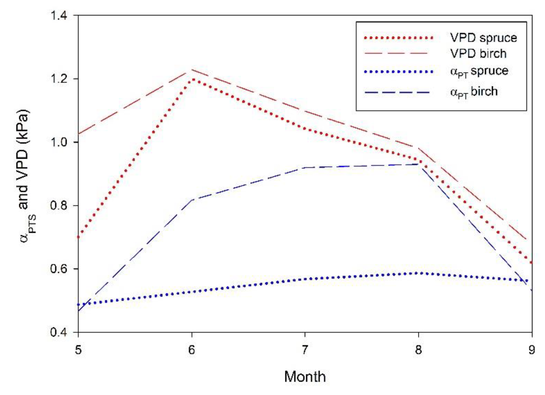
2.2. Adjustments to the Effective Priestley–Taylor and the Soil Heat Flux Configurations for Boreal Forest Settings

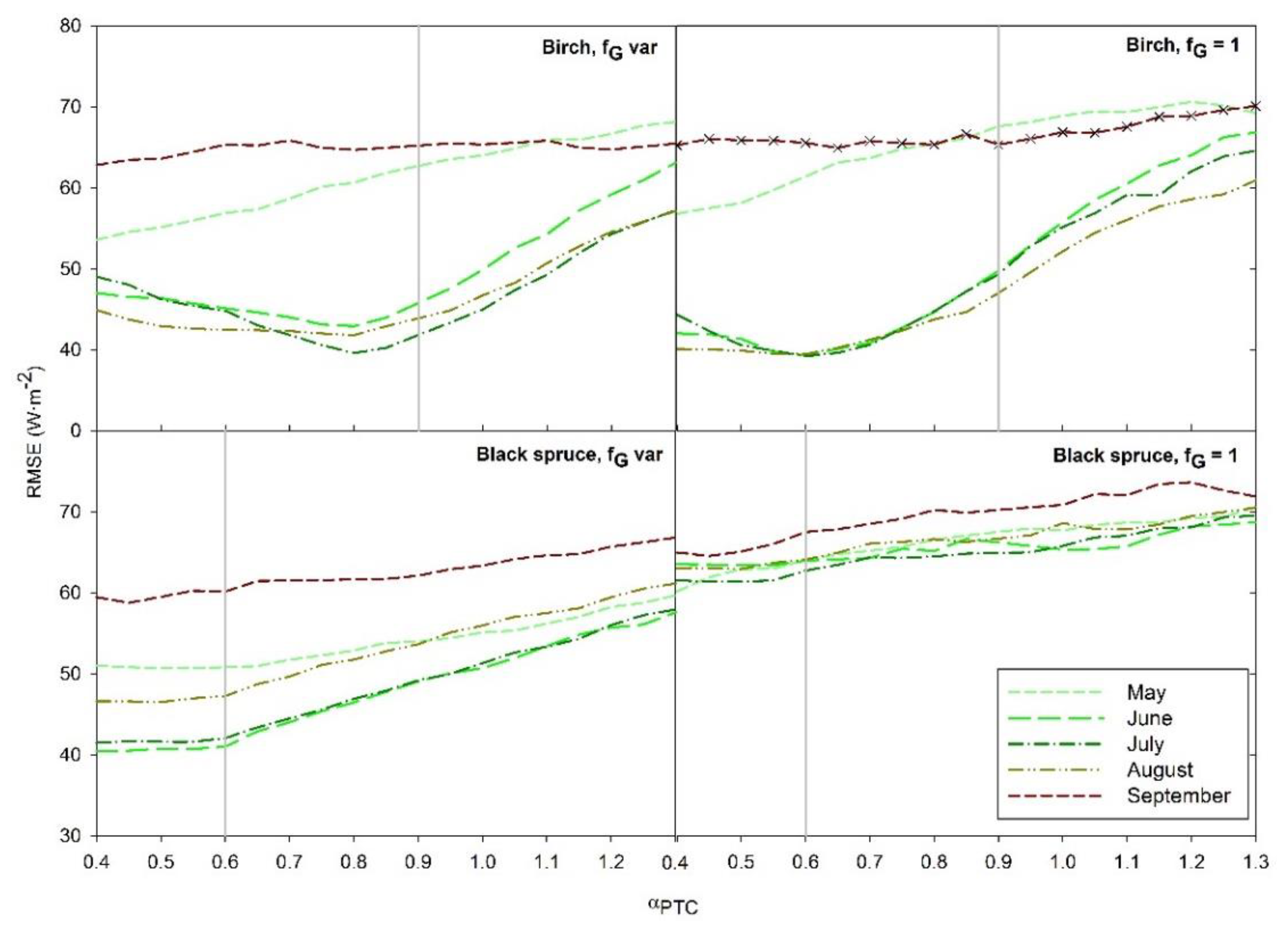
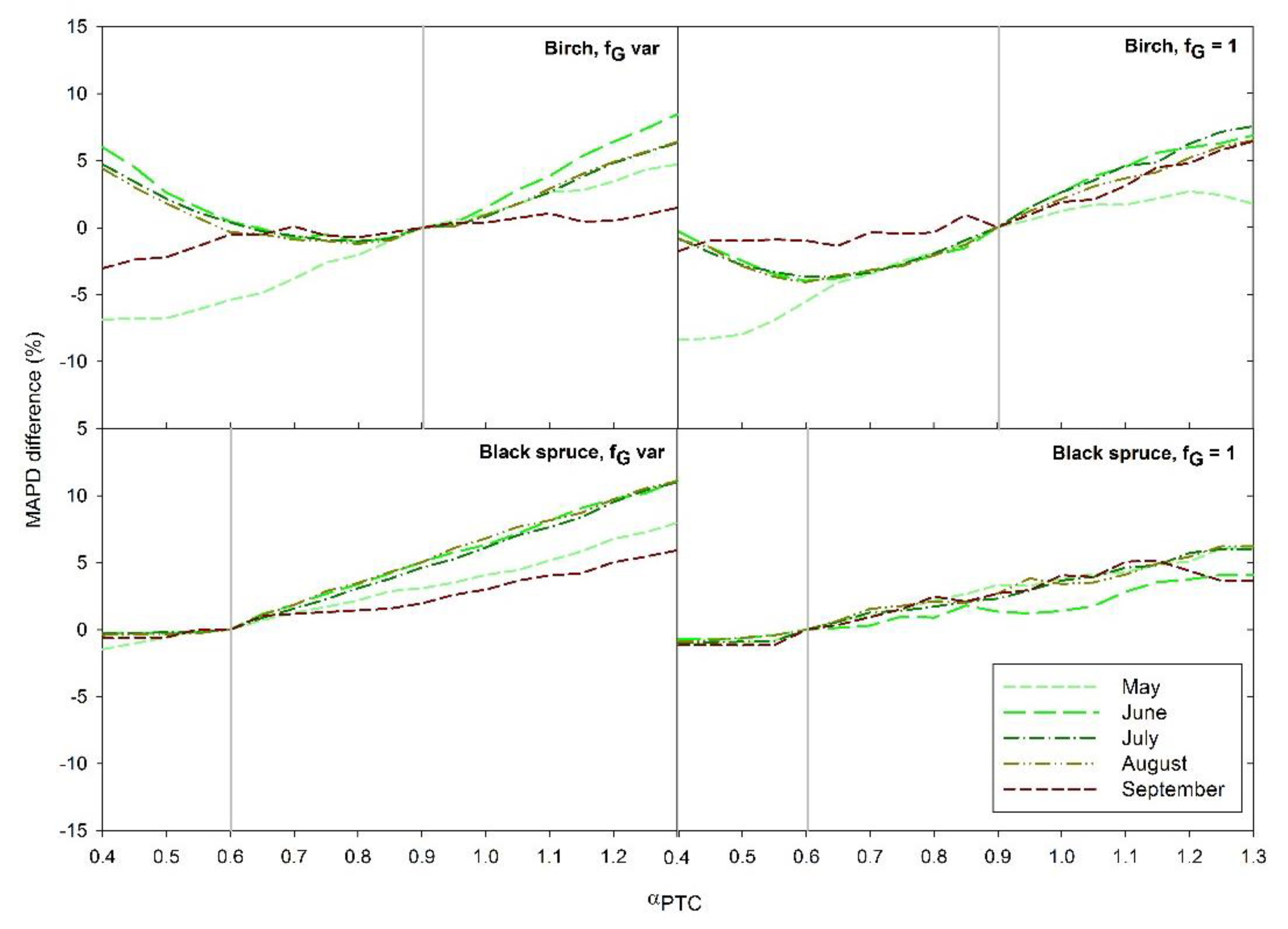
2.2.1. TSEB Priestley–Taylor Coefficient Modifications and Evaluation

To estimate the LE flux from the canopy component, TSEB internally changes its initial αPTC values of 1.26 to allow an acceptable partitioning between LEC and LES under stressed vegetation conditions. The initial value of αPTC is down-adjusted when TSEB results in negative values for LES, given that condensation on the soil is unlikely to occur during the day [28]. This condition typically occurs if the potential transpiration flux is too high to be consistent with the observed surface temperature. The canopy temperature estimate in is too low, resulting in a high soil temperature derived from Equation (1). This leads to high soil sensible heat (Equation (10)) exceeding the available energy at the soil surface, and hence LES < 0 result from Equation (13). When this non-physical condition is encountered midday, it is assumed that the canopy is stressed and αPTC is iteratively reduced until LES values are higher than 0. This iterative scheme works well in ecosystems where canopy values of αPTC are relatively conservative under unstressed conditions [39], while for stressed canopies where the soil surface is usually dry, a LES value close to zero is a reasonable assumption [40].
In croplands, rangelands and temperate forests where the TSEB model was previously evaluated, the assumptions that (a) the vegetation is fully green (fG = 1); and (b) that the maximum potential (unstressed) transpiration rate is obtained with αPTC = 1.26 [36]; yielded successful results. However, Ref. [41] suggested that for canopies that are more conservative in their water use (not transpiring at the potential rate) or not completely green, αPTC and fG need to be adjusted to yield a reasonable LE partitioning. Moreover, refs. [27,42] and also found acceptable TSEB results for natural vegetation and Arctic tundra using initially a lower αPTC, suggesting that lower values for natural ecosystems with vegetation adapted to water-limited environments would be more realistic and yield more accurate LE values.
In many boreal forests, tree growth is limited by low precipitation and low temperatures that in turn restrict photosynthetic capacity and reduce root hydraulic conductivity and stomatal conductance, resulting in low-LAI canopies that exert a significant resistance to transpiration [43]. Moreover, conifer forests (such as black spruce forests) growing in upland regions of the boreal zone, evaporate at rates between 25 and 75% of equilibrium evaporation defined as a special case when αPTC = 1. On the other hand, evaporation rates from deciduous forests (such as birch forests) may approach equilibrium rates [43]. The standard TSEB parameterization of αPTC, assuming an initial value of 1.26, may not reach the low values resulting the controls of climate and vegetation on the energy exchange of boreal forests.
Although specific values of αPTC for the boreal forest are not found in the literature, αPT measurements for the whole system (canopy and soil) and hereinafter referred to as αPTS, are available for deciduous forest and boreal conifer evergreen systems [43,44,45,46,47,48,49,50,51] with an average value of 0.6 ± 0.17 and 0.9 ± 0.2, respectively, and representative for black spruce and birch forests. Moreover, αPTS also may show seasonal variations that can vary significantly with LAI, vapour pressure deficit (VPD), and soil moisture [52].
For modelling purposes, deciduous forest and boreal conifer evergreen averaged αPTS values together with the original TSEB αPTC value of 1.26 were used to estimate the most appropriate initial αPTC value for TSEB. Moreover, to capture seasonal phenology in green vegetation cover, a simple vegetation index ratio proposed by [43] was applied:
f G = 1.2   [ E V I / N D V I ] ,   0     f G     1
Additionally, to evaluate the effect of αPTC and fG on the latent heat estimation, a sensitivity analysis on αPTC and fG was conducted [42]. This consists in running TSEB with αPTC values increasing at 0.05 intervals from 0.4 to 1.3 for both black spruce and birch, respectively, with (a) the fG derived from the EVI and NDVI ratio and (b) a fG = 1 assuming active transpiration from the canopy.
Finally, αPTS measurements were computed to (1) analyze its seasonal behavior at both flux towers as a function of soil moisture, VPD and phenology, and (2) compare its value with results from the sensitivity analysis. Values of αPTS were computed using the flux tower data using the following equation:
α P T S = E / E e q
where E and Eeq are the measured evaporation from the flux towers and the equilibrium evaporation rate, respectively, with Eeq computed as follows:
E e q = ( Δ / ( Δ + γ ) ) ( R n G ) ,

2.2.2. Modifications and Evaluation for Soil Heat Flux

For soil heat flux estimation, a cG mean value of 0.3 is not likely appropriate for boreal forest settings due to forest floor residue and subcanopy moss and vegetation For tundra vegetation, large errors using a cG of 0.3 were also found [27]. Although there is a lack of specific cG values for spruce or deciduous forests in the literature, data derived from different studies in summer months and in similar boreal settings [43,44,47,50,53,54,55,56,57] allowed computing a mean value of cG for spruce and deciduous forests of 0.07 ± 0.03.
Although this approach was successfully applied for croplands, a new approach in Arctic tundra [27] to estimate G using the relationship between G and TRAD in Equation (18) yielded better agreement than using both constant or phase shifted cG values in Equation (14). This methodology also accounted for a phase shift by using the maximum value of cGT in Equation (14) instead of cG as follows:
c G T = G / T R A D
Thus, to estimate G, a modified cG value for the boreal forest of 0.07 was applied to the original TSEB formulation (Equation (14)). Moreover, the approach using the G-TRAD relationship (Equations (14) and (18)) was also fitted and evaluated with 60% and 40% of the flux tower dataset, respectively, and then applied to the full dataset at the black spruce and birch forest sites.

3. Study Area and Instrumentation

Two experimental sites were established from 2011 to 2012 in two of the main covers of the boreal forest, birch and black spruce forests, for the TSEB calibration and evaluation in boreal settings (Figure 1). The first setting, located at the North Campus of the University of Alaska Fairbanks (UAF; 64°51′56.803″N and 147°50′34.154″W), was installed in a needle-leaf black spruce forest with discontinuous permafrost. The overstory was predominantly black spruce (Picea mariana) with a canopy cover around 60% and a mean tree height of about 5 m. The understory is covered by shrubs (Betula nana, Ledum palustre, Alnus incana) and mosses (Sphagnum spp.). The flux tower was installed in 2011 with a total height of 23 m. a.g.l. Unfortunately, in 2014, the thaw of discontinuous permafrost around the flux towers caused tower integrity issues and tower height was reduced to 15 m. This led to a data gap of around 1 year, from July 2014 to June 2015.
The second setting was located at the Caribou Poker Creeks Research Watershed (CPCRW; 65°10′17.962″N and 147°28′17.137″W) in a deciduous paper birch (Betula neoalaskana) forest with a summer canopy cover around 95% and a mean tree height of about 16 m and a tower height of 23 m a.g.l. In this case, the understory is covered by shrubs (Betula nana, Ledum palustre) and mosses (Sphagnum spp.).Both field sites were equipped with a sonic anemometer, a gas analyzer operating at 20 Hz sampling rate, four-component net radiometer sensor and air temperature sensors at different heights (for further details on tower instrumentation see [58]). Ground heat was monitored at both sites by temperature and soil moisture probes and heat flux plates installed in the subsurface soil layers. Precipitation was measured at black spruce flux tower using a rainfall gauge. At the birch flux tower rainfall data from another meteorological station operated by the CPCRW long-term ecological research (LTER) network were used. Both towers were operated year-round, although some data gaps were present in deep winter due to power shortage or flux tower access limitations due to harsh weather conditions.

4. Model Input and Evaluation

The TSEB model was run in two modes: (a) using local measurements of surface temperature as input, and (b) using remote sensing of surface temperature estimates, and in both cases with meteorological data from the flux towers (air temperature, atmospheric pressure, wind speed, vapor pressure, and solar radiation). For both modes, vegetation properties such as fG and LAI were derived using remote sensing estimates. As a local source of surface temperature, TRAD, upwelling longwave data from the four component net radiation sensor were converted to TRAD [58]. For model runs using satellite-based TRAD, Terra/Aqua MODIS TRAD from Terra/Aqua MODIS LST product (MOD11) was used. To ensure the best quality data, only high quality LST data with an average error ≤1 K and with a view-angle up to 35 degrees according to quality flags of the product were considered. Pixel selection was done by a footprint analysis based on [59] methodology accounting for 90% of the flux tower footprint cover.
To evaluate RN, LE, H, and G TSEB model output, a conservative approach was taken to screen out the 30-min time-step flux tower data to ensure inclusion of only high-quality data. To cover the whole growing season at both sites, only snow-free data between May to September from 2012 to 2016 data were considered, identified using Terra/Aqua MODIS snow cover products. Then, daily rainfall events were also removed. Finally, two more filters to ensure data quality and daytime conditions were applied: (a) a 30-min timescale energy closure > 70% and, (b) RN > 100 W·m−2. This resulted in a total of 289 days at UAF and 392 at CPCRW. It is important to note that the final evaluation dataset was substantially reduced due to the large amount of rainy days, which are common in the boreal forest.

4.1. Micrometeorological Data Processing

High-frequency (20 Hz) eddy covariance raw data collected at both sites were screened to identify and remove nonphysical values and data spikes [60]. Half-hour mean wind speed and direction were then computed after wind velocity components of the coordinate system were rotated to align with prevailing wind direction [61,62]. Sonic temperature data was then converted to air temperature by adjusting for humidity effects [63] and corrected for sensor displacement and frequency response attenuation [64,65]. The moisture and carbon dioxide fluxes were then corrected for the effects of buoyancy and water vapor density [66] and as a result, 30-min turbulent fluxes were calculated. The daily average energy balance closure for the selected period at both black spruce and birch sites was 0.87 and 0.91, respectively, which is in agreement with many other eddy covariance studies [67]. To apply the surface energy balance expression, residuals were allocated to latent heat flux [68], ensuring the closure of the energy balance and further comparability with modelled fluxes. Corrections to account for soil heat storage were applied on the soil heat flux plates measurements together with soil bulk density sampled at each site (1244 and 1208 kg·m−3 for birch and black spruce, respectively) as well as soil moisture and soil temperature probes [69,70].

4.2. Remote Sensing Estimates of Vegetation Properties

The TSEB configuration used in this study requires estimates of LAI and fG derived from EVI and NDVI. LAI field measurements were obtained intermittently at both sites during the study time period with a Decagon LP-80 Ceptometer using 50 regular samples within a 200 m radius nearby the flux towers. However, in-situ measurements did not cover the growing season to senescence, and field measurements of NDVI or EVI were unavailable. To produce temporally smoothed NDVI, EVI and LAI data, TIMESAT [71] was used together with MODIS 4-day LAI product (MCD15A3H), both MODIS daily reflectance product at 250 and 500 m (MOD09GQ and MOD09GA, respectively) and their quality flags (see [27] for more details). The clumping factor Ω (Equation (2)) was set to 0.8 and 0.7 for birch and black spruce sites, respectively, based on forest inventories and image photointerpretation.

5. Results and Discussion

In this section, we present an evaluation of daytime instantaneous surface energy flux estimates from TSEB over all-sky conditions using local and remotely sensed inputs of TRAD, and applying different values of αPTC and fG.

5.1. Model Performance Using In-Situ TRAD Measurements

For both flux datasets used here, measured G was a relatively small term with a daytime average value between 9 and 17 and W·m−2 for the black spruce and birch sites, respectively, in comparison to daytime average RN of around 321 W·m−2 at both sites. Fitting Equation (14) for cG for both spruce and deciduous sites resulted in values for cG, B and S of 0.07, −7200 and 250,000, respectively. When the variable cTG computed from Equation (18) replaced cG in Equation (14), fitted values for cTG, B and S were 0.9, −7200 and 200,000, respectively. In both cases, a 2 h phase shift after the maximum TRAD at noon showed a negligible influence on the results when applying a B variation of ±15,000 s.
Using cG = 0.07 in Equation (14) for G estimation, model estimates showed lower agreement with observed soil heat fluxes at the black spruce site, with R2, the mean absolute percent difference (MAPD), the root mean square error (RMSE) and mean bias error (MBE) values of 0.1, 95%, 19 W·m−2 and 17 W·m−2, respectively, and with R2, MAPD, RMSE and MBE values of 0.05, 98%, 26 W·m−2 and 24 W·m−2 for the birch site (results not shown in Table 2). When G was estimated replacing cG in Equation (14) with cGT estimated from Equation (18) a better agreement was obtained, reducing by 50% discrepancies with measured G compared to the standard TSEB approach using a constant cG (Table 2). This is also in agreement with [27] who found better performance using the G-TRAD relationship for Arctic tundra. In this case, modeled G had negligible bias compared to observations, with R2, MAPD, RMSE and MBE values of 0.47, 44%, 5 W·m−2 and 1 W·m−2, the for black spruce site, and with R2, MAPD, RMSE and MBE values of 0.65, 47% 7 W·m−2 and −3 W·m−2, for the birch site (Figure 2 and Table 2). Although RMSE is similar at both sites, the lower observed soil heat flux at the black spruce site, due a thicker moss layer that increases soil insulation, led to a higher MAPD value for the birch site.
Modeled RN yielded comparable results at both sites with a high correlation and almost negligible bias, with values of MAPD of around 5%, an RMSE from 18 W·m−2 to 22 W·m−2, an MBE from 0 W·m−2 to 4 W·m−2 and an R2 of 0.98 (Figure 2 and Table 2). These results are similar to those found in Arctic tundra using the same RN modelling configuration [27]. This suggests that this model configuration may be also applied for the whole growing season in all-sky conditions for boreal forest settings. Moreover, they are also aligned with previous TSEB model findings in different cover types and for clear sky in which a 5% of error percentage (MAPD) was described [31,39,40,41,72,73,74].
Turbulent heat fluxes, H and LE, estimated with model modifications in G and RN, yielded reasonable agreement with 30-min observed fluxes when αPTC was adjusted for boreal vegetation (0.6 and 0.9 for black spruce and birch settings, respectively), and poorer agreement using the original αPTC of 1.26, with an RMSE difference between both configurations of 23 W·m−2 to 28 W·m−2 (Table 2 and Figure 2).
For birch and black spruce, RMSE for LE and H for the original αPTC configuration ranged from 64 to 77 W·m−2, while for the adjusted αPTC configuration LE and H ranged from 41 to 49 W·m−2, errors comparable to those described in other studies [75], and according to [76] after daily integration of instantaneous daytime fluxes the errors will tend to be reduced on the order of 10–15%. The error percentage (MAPD) in LE and H using the adjusted αPTC values were also reduced from 32% to 39% to less than 25%. For both original and adjusted αPTC values, the model tended to overestimate LE and underestimate H. Model LE and H under- and overestimation may be also explained due to the lack of instrument closure and methodological uncertainties, insufficient estimation of storage terms, unmeasured advective fluxes, landscape scale heterogeneity or instrument spatial representativeness, among others [67,68,70,77,78].
In comparison, Sanchez et al. [79] reported similar RMSE results of around 50 W·m−2 for both H and LE in a Finnish boreal forest over a two-month summer validation study with a simplified version the TSEB. These results suggest that the adjusted lower αPTC values for deciduous and coniferous forest covers better describe controls of climate and vegetation on the energy exchange of boreal forest under current conditions. This is in line with other studies in deciduous and coniferous forests [27,41,42,49] suggesting that vegetation-type adjusted values of αPTC could yield more accurate H and LE values in cases where the natural vegetation is adapted to the local climate conditions. Although a vegetation class-dependent value of αPTC might seem disadvantageous as ancillary land use cover or vegetation cover information is needed, current initiatives in mapping the boreal forest vegetation types [80,81] should enable use of adjusted values of αPTC, thus, decreasing the bias associated with using a universal value of αPTC of 1.26 for regional applications.

5.2. Evaluation of Remote Sensing Vegetation Properties Estimates

Time series of LAI from the MODIS product used to partition soil and canopy temperatures (Equation (2)) captured seasonal dynamics from green-up to senescence for the whole period at both flux towers (Figure 3). Moreover, comparison with in-situ field estimates of LAI (not originally intended for LAI MODIS product evaluation) yielded a reasonable error with a RMSE of 0.7 and 0.6 and an MBE of −0.7 and 0.2 at the black spruce and birch sites, respectively. For black spruce, fG computed using Equation (15) a good correspondence with LAI dynamics for the whole growing period (May to September) was found. The birch site showed a similar behavior from June to August. However, in May and September the pattern was different due to an already green understory with low LAI in leaf-out and senescence (Figure 3 lower panel and especially visible in 2013).

5.3. Seasonal Dynamics in Surface Energy Fluxes

Monthly estimation of RN, LE, H, and G with adjusted αPTC and the modified G configuration showed an acceptable overall agreement with observations from June through August (months with the greatest vegetation activity in the boreal forest), with RMSE values lower than 50 W·m−2 and an mean MAPD around 23% (Table 3 and Table 4, and Figure 4). However, model performance deteriorated to some extent at leaf-out and at senescence. During these periods, LE was overestimated by the model, and H underestimated. This may be related to unreliable estimates of fG or αPTC at the start of leaf-out and at the end of the senescence periods.
Due to the lack of αPTC values in the literature, a first approach to understand its seasonal behavior is assuming αPTS computed in Equations (16) and (17) with flux tower data as representative of the αPTC behavior. Results showed that from June to August αPTS values were similar to other studies and used in this study to model turbulent fluxes with a value of 0.89 ± 0.05 for birch and 0.56 ± 0.03 for black spruce (Figure 5). However, in the leaf-out and senescence (May and September) αPTS yielded lower values. For black spruce, values were 0.49 and 0.56, similar to the reference αPTC value of 0.6 used to estimate LE. However, for birch values were almost half of the reference αPTC value of 0.9 that was used, 0.47 and 0.53, respectively, similar to those reported in other boreal deciduous forests [82]. In both cases, αPTS behaved according to VPD.
Moreover, results from the sensitivity analysis (Figure 6 and Figure 7) for αPTC showed similar temporal behavior to that from αPTS values (Figure 5). For black spruce, the lowest error (RMSE) in LE estimation was found with an αPTC value of around 0.55 together with a variable fG using the EVI and NDVI relationship (Equation (15)). The RMSE ranged from 40 W·m−2 to 50 W·m−2 for the whole growing season. Using a constant fG value of 1.0, the error increased for all LE estimations for the whole period suggesting that a reduction in αPTC alone was not enough to properly capture LE dynamics.
For birch, lower errors were found from June to August when a αPTC value of 0.8 and a variable fG were applied (Figure 6). However, in May and September, there was an improvement in LE when lower αPTC values of around 0.5 and a variable fG were applied of around 15 W·m−2 and 2 W·m−2, respectively. This behavior is similar to αPTS for the whole system (soil + canopy) seasonal dynamics (Figure 5). When fG was considered to be 1, the overall error was higher. Moreover, lower values of αPTC of around 0.6 were needed to obtain similar values to those using a variable fG. This led to more unrealistic αPTS values compared to those found in Figure 5 and reported in the literature.
To further evaluate the sensitivity of choice of αPTC on LE estimation, differences in MAPD obtained using a range in αPTC from that obtained using the reference values of 0.6 and 0.9 for black spruce and birch, respectively, are shown in Figure 7. MAPD for black spruce was almost insensitive to use of lower values of αPTC, and errors increase steadily for αPTC above the reference value. This suggests that an initial αPTC value of 0.6 should be used for modeling black spruce water use. For all values of αPTC, applying a variable fG improved the LE estimation as already reported by [41]. Birch showed similar pattern from June to August, with an αPTC of around 0.8. However, the error difference within a αPTC interval from 0.8 to 1 in absolute value was around 1%, steadily increasing when lower and higher values were applied. This suggests that an initial αPTC mean value of 0.9 found in the literature may be applied to model LE regionally for birch. However, in May, αPTC lower values of 0.5 yielded a 7% improvement while in September of around 2%, suggesting that a value of 0.5 would be more appropriate to estimate LE. This moderate improvement in September could be related to the issues in capturing fG dynamics at the end of the season due to an already green understory but with low evaporation rates, although more research is needed.
Model performance in estimating RN was comparable at both sites with a high correlation (R2 from 0.95 to 0.99) and a low MAPD of around 5% for most of the season. For G, seasonal values at both sites had lower values and narrow range compared to the remaining surface energy fluxes which makes it more difficult for the model to be able to capture the seasonal dynamics. However, the proposed method to estimate G was able to capture the seasonal dynamics at both sites from June to August, corresponding to the growing season peak, yielding lower MAPD results.

5.4. Model Performance Using Remote Sensing TRAD Estimates

As a first step towards regional implementation of the modified TSEB model over the boreal region, TRAD from satellite data was used as input. In addition boreal-specific modifications to αPTC and G were implemented using cGT (Equation (18)) instead of cG in Equation (14), thus allowing for a phase shift. Modifications in αPTC included an αPTC value for the whole season of 0.6 for black spruce, and an αPTC value of 0.5 in May and September, and 0.9 from June to August for birch, were applied to evaluate model performance. Overall results (Table 5 and Figure 8) showed commensurate agreement for RN and G than those using TRAD from the pyrgeometer at each site, yielding LE and H slightly higher RMSE values but similar error percentage. These results suggest that regional implementation of TSEB for the boreal forest with the model modifications applied in this study are adequate to retrieve surface energy fluxes. RN yielded similar results compared to model application with pyrgeometer TRAD with an RMSE and an MAPD of around 20 W·m−2 and 4% for both black spruce and birch sites, respectively. G also showed similar results with an RMSE and an MAPD of around 7 W·m−2 and 40% for both settings.
For both boreal sites, LE and H modeled with remotely sensed TRAD yielded slightly higher RMSE of around 65 and 55 W·m−2, respectively, although the MAPD was consistent to those results found with pyrgeometer data of around 30 and 20%, respectively. Thus, modifications in αPTC and fG together with remote sensing estimates of TRAD suggests that TSEB can be applied regionally to estimate turbulent fluxes. However, an error and bias increase compared to local estimates of TRAD using flux tower data might be explained in part by biases in TRAD-TA, due to atmospheric and emissivity corrections, sensor biases or unrepresentative TRAD at 1 km resolution relative to the flux tower footprint and meteorological forcing data. Thus, when applied regionally, TSEB is typically performed in time-differential mode because time-differences in TRAD reduce errors caused by uncertainty in atmospheric correction and emissivity for determining the absolute TRAD value.
Comparison of MODIS TRAD estimates with flux tower TRAD observations yielded a RMSE and a MBE of 1.9 K and −1.3 K at the birch site, respectively, and a RMSE and a MBE of 2.2 K and −1.3 K, respectively, at the black spruce site (Figure 9), thus, underestimating ground estimates of TRAD. This resulted in an increased bias and error in LE and H estimation lowering the final agreement. Therefore, to avoid an increase in bias on TRAD, for circumpolar boreal regions an alternative time-differential TSEB technique using a dual-time difference (DTD model) in observed TRAD and air temperature [41,83] will be implemented adding the model modifications found in this paper.
Moreover, it is worth noting that for the whole study period, there was a limited amount of TRAD data from MODIS. Although this is in part due to the constraints of data selection applied for the TSEB evaluation, clouds are an important source of contamination that hamper satellite applications using optical and thermal wavebands in the Arctic and boreal ecosystems. For instance, only 5% of the selected dataset was considered to be completely cloud-free. Thus, for regional applications of surface energy fluxes retrieval using remote sensing thermal infrared data as TRAD, a multiplatform approach from several polar satellites may be needed to increase the frequency of useable data, particularly during the growing season. Guzinski et al. [41] demonstrated good performance of a MODIS-driven DTD implementation over monitoring sites in Denmark, which have frequent cloud cover and are not well-sampled by polar orbits using combined Terra and Aqua satellite overpasses. Fortunately, near the poles, moderate resolution polar-orbiting thermal imaging systems, including Terra/Aqua MODIS, NOAA AVHRR, NPOES VIIRS, Sentinel 3 or microwave systems such as Aqua AMSR-E Ku-band [84] provide multiple image acquisitions per day, that allow mimicking a coarse temporal resolution geostationary system but at higher spatial resolutions increasing the likelihood of thermal infrared cloud-free pixels.
For regional implementation, meteorological inputs (air temperature, atmospheric pressure, wind speed, vapor pressure, and solar radiation) can be obtained from the NCEP North American Regional Reanalysis dataset, available at a spatial resolution of 32 km and a temporal resolution of 3 h. Land cover maps required to assign initial αPT values can be obtained from current land cover initiatives [80,81], or using the Terra/Aqua MODIS land cover product or the USGS National Land Cover Database (https://www.usgs.gov/centers/eros/science/national-land-cover-database). Although black spruce and birch are the two main covers of the boreal forest of interior Alaska, other minor covers representative of wetland ecosystems such as fen are also present in the boreal forest and can be parameterized by [27]. Finally, vegetation properties such as fG or LAI can be derived by temporally smoothing Terra/Aqua NDVI, EVI and LAI product data.

6. Conclusions

Modifications of a two-source energy balance (TSEB) model were applied to estimate daytime surface energy fluxes on two main vegetation types of the boreal forest of interior Alaska, black spruce and birch. An extensive model evaluation from leaf-out to senescence from 2012 to 2016 using local thermal data from the flux towers and Terra/Aqua MODIS remote sensing estimates as inputs was conducted. Model modifications included: (a) RN estimation for all-sky conditions (overcast and cloud-free), (b) a refined model for soil heat flux (G) previously applied for Arctic tundra and based on the TRAD-G relationship, and, (c) a αPTC parameterization for estimating canopy transpiration adopting an initial value of 1.26 and adjusted values of 0.6 and 0.9 for black spruce and birch, respectively.
Results showed that TSEB can appropriately model surface energy fluxes in the boreal forest from leaf-out to senescence. The modified model for soil heat flux estimation (G) yielded lower errors half that from the standard TSEB formulation. The RN model configuration for all sky conditions yielded similar errors to previous studies only for clear-sky conditions. TSEB modifications for boreal settings with adjusted αPTC provided turbulent heat flux estimates of H and LE with a mean RMSE value less than 50 W·m−2 and error percentage of around 23% in comparison with flux tower data that is comparable with errors typically described by other studies modelling surface energy fluxes. Results with the original αPTC configuration showed higher RMSE suggesting that vegetation and climate-type adjusted values of αPTC indicating different transpiration response to atmospheric forcing for black spruce, and birch would yield more accurate H and LE values.
A sensitivity analysis on αPTC and fG showed that for black spruce, an initial αPTC value of 0.6 together with a variable fG can be applied to estimate LE regionally for the whole growing season. For birch, although an initial αPTC value of 0.9 was successfully applied from June to September, seasonally adjusted values were also needed in the leaf-out and senescence periods with a αPTC value of 0.5 due to the influence of understory phenology.
When remote sensing estimates of TRAD were used as input, TSEB yielded slightly higher RMSE of around 60 W·m−2 for turbulent heat fluxes (H and LE), which was mainly attributed to an increase in bias compared to tower-based TRAD measurements. However, similar errors for G and RN were found compared with tower-based TRAD measurements.
For vegetation properties, Terra/Aqua MODIS vegetation indices (NDVI and EVI) and LAI time series fitted with TIMESAT provided reasonable estimates of LAI and fG, resulting in the model reproducing with good fidelity the temporal trends of energy partitioning together with boreal forest seasonality from leaf-out to senesce. This fact is particularly important for regional applications as LAI and fG field observations are not always available.
For regional applications, future work will be focused on incorporating the TSEB model improvements in boreal forest settings described in this study within the Atmospheric Land EXchange Inverse (ALEXI) surface energy balance regional modelling framework by using long time series of remote sensing estimates. It is also worth noting that for the whole study period, limited cloud-free MODIS thermal data were available. As clear-sky sky data are needed for regional applications, a multiplatform approach from several satellites polar satellites such as Terra/Aqua MODIS, NOAA AVHRR, NPOES VIIRS. Alternatively, microwave-derived TRAD using Aqua AMSR-E will be also needed to increase the likelihood of cloud-free data during non clear-sky conditions.

Author Contributions

Conceptualization J.C. and A.P.; methodology, J.C., W.P.K., M.C.A. and J.G.A.; validation, J.C. and A.P.; formal analysis, J.C., W.P.K. and M.C.A.; investigation, J.C.; resources, A.P., J.C. and R.G.; data curation, J.C.; writing—original draft preparation, J.C.; writing—review and editing, J.C., A.P., W.P.K., M.C.A., R.G. and J.G.A.; visualization, J.C.; supervision, J.C. and A.P.; project administration, A.P. and J.C.; funding acquisition, A.P., R.G. and J.C. All authors have read and agreed to the published version of the manuscript.

Funding

These research activities are based in part upon work supported by the Alaska NASA EPSCoR Program (awards NNX13AB28A and NNX10AN02A, and project titles “Estimating Spatio-Temporal Variability in Evapotranspiration in Interior Alaska Using Field Measurements, Modeling and Remote Sensing” and “Estimating year-round surface energy fluxes in Alaska Arctic and sub-Arctic watershed through remote sensing and field measurements”, respectively), Alaska EPSCoR NSF (award #OIA-1208927 and project title: “Integrating multiplatform remote sensing and field data to estimate energy fluxes under snow conditions in Arctic ecosystems”), the Alaska Space Grant Program, and the state of Alaska.

Acknowledgments

Authors would like to thank Jamie Hollingsworth at the Institute of Arctic Biology of the University of Alaska Fairbanks for his help accessing the CPCRW LTER site and flux tower installation logistics and Fochessato and Starkenburg for their help setting-up and maintaining the flux towers. Special thanks to Patrick Graham for his help in flux tower maintenance LAI field data collection. Finally, the authors would also like to thank Watcharee Ruairuen and Mingchu Zhang at the College of Natural Science and Mathematics of the University of Alaska Fairbanks for their help in processing the soil samples to obtain the soil bulk density. USDA is an equal opportunity provider and employer.

Conflicts of Interest

The authors declare no conflict of interest. The funders had no role in the design of the study; in the collection, analyses, or interpretation of data; in the writing of the manuscript, or in the decision to publish the results.

Appendix A. Summary of Equations Used to Estimate Aerodynamic Resistances in TSEB

In this appendix, the resistances involved in Equation (9), Equations (10) and (11) are summarized. RA is the aerodynamic resistance in the surface layer computed from the stability-corrected temperature profile equations (s·m−1) defined as:
R A = [ ln ( ( z U d O ) / z O M ) Ψ M ] [ ln ( ( z T d O ) / z O M ) Ψ H ] k 2 u
where dO is the displacement height, U is the wind speed measured at height zU, k is von Karman’s constant (≈0.4), zT is the height of the TA measurement, ΨM and ΨH are the Monin–Obukhov stability functions for momentum and heat, respectively, and zOM is the aerodynamic roughness length. Both dO and zOM were estimated using LAI and canopy height (hC) as follows [85,86]:
d O = 0.7 ( 1 ( 5 n ) ( 1 e ( 3.3 n ) ) ) h C
where n is the within-canopy wind speed profile extinction coefficient parameterized as:
n = C d   L A I 2 ( u * u ( h ) ) 2
where Cd is the drag coefficient of the foliage elements with a value of 0.2, and the ratio u * /u(h) is parameterized as:
u * u ( h ) = 0.360 0.264   e ( 15.1 C d L A I )
Finally, zOM is defined as:
z O M = ( 1 d O ) e 0.4 / u * u ( h )   h C
RS is the resistance to the heat flow in the boundary layer above the soil (s·m−1) defined as:
R S = 1 a + b U S
where a′ ≈ 0.004 m·s−1, a′ ≈ 0.012 m·s−1, US is the wind speed (m·s−1) at the height above the soil surface where the effect of the soil surface roughness is minimal (~5 cm) and estimated from the [87] wind attenuation model through the canopy layer (see Equation (A8)).
Finally, RX is the total boundary layer resistance of the vegetation leaf layer (s·m−1) defined as:
R X = C L A I ( S U d o + Z o m ) 1 / 2
where C′ is derived from weighting a coefficient in the equation for leaf boundary layer resistance (assumed a constant ~90 s1/2 m−1) and S is leaf size (m). Ud+Zm is given by:
U d o + Z o m = U C   e x p [ a ( 1 d o + Z o m h C ) ]
where UC is the wind speed at canopy height (hC) and a is the wind attenuation coefficient of the [87] wind attenuation model which is a function of LAI, hC and leaf size. For a full description of the TSEB resistance formulations see [28,31,32].

References

  1. Serreze, M.C.; Barry, R.G. Processes and impacts of arctic amplification: A research synthesis. Glob. Planet Chang. 2011, 77, 85–96. [Google Scholar] [CrossRef]
  2. AMAP. Arctic Climate Issues 2011: Changes in Arctic Snow, Water, Ice and Permafrost; Swipa 2011, Overview Report; Arctic Monitoring and Assessment Programme (AMAP): Oslo, Norway, 2012; p. 96. [Google Scholar]
  3. Bates, B.C.; Kundzewicz, Z.W.; Wu, S.; Palutikof, J.P. Climate Change and Water; Technical Paper of the Intergovernmental Panel on Climate Change; IPCC Secretariat: Geneva, Switzerland, 2008. [Google Scholar]
  4. Bhatt, U.S.; Walker, D.A.; Raynolds, M.K.; Comiso, J.C.; Epstein, H.E.; Jia, G.S.; Gens, R.; Pinzon, J.E.; Tucker, C.J.; Tweedie, C.E.; et al. Circumpolar arctic tundra vegetation change is linked to sea ice decline. Earth Interact. 2010, 14, 1–20. [Google Scholar] [CrossRef] [Green Version]
  5. McGuire, A.D.; Wirth, C.; Apps, M.; Beringer, J.; Clein, J.; Epstein, H.; Kicklighter, D.W.; Bhatti, J.; Chapin, F.S.; de Groot, B.; et al. Environmental variation, vegetation distribution, carbon dynamics and water/energy exchange at high latitudes. J. Veg. Sci. 2002, 13, 301–314. [Google Scholar] [CrossRef]
  6. Verbyla, D. The greening and browning of alaska based on 1982–2003 satellite data. Glob. Ecol. Biogeogr. 2008, 17, 547–555. [Google Scholar] [CrossRef]
  7. Yang, F.; Kumar, A.; Schlesinger, M.E.; Wang, W. Intensity of hydrological cycles in warmer climates. J. Clim. 2003, 16, 2419–2423. [Google Scholar] [CrossRef]
  8. Calef, M.P.; Varvak, A.; McGuire, A.D.; Chapin, F.S.; Reinhold, K.B. Recent changes in annual area burned in interior alaska: The impact of fire management. Earth Interact. 2015, 19, 1–17. [Google Scholar] [CrossRef] [Green Version]
  9. Bintanja, R.; Selten, F.M. Future increases in arctic precipitation linked to local evaporation and sea-ice retreat. Nature 2014, 509, 479–482. [Google Scholar] [CrossRef]
  10. Wendler, G.; Shulski, M. A century of climate change for fairbanks, alaska. Arctic 2009, 62, 295–300. [Google Scholar] [CrossRef]
  11. Osterkamp, T.E.; Jorgenson, M.T.; Schuur, E.A.G.; Shur, Y.L.; Kanevskiy, M.Z.; Vogel, J.G.; Tumskoy, V.E. Physical and ecological changes associated with warming permafrost and thermokarst in interior Alaska. Permafr. Periglac 2009, 20, 235–256. [Google Scholar] [CrossRef]
  12. Vörösmarty, C.J.; Hinzman, L.D.; Peterson, B.J.; Bromwich, D.H.; Hamilton, L.C.; Morison, J.; Romanovsky, V.E.; Sturm, M.; Webb, R.S. The Hydrologic Cycle and its Role in Arctic and Global Environmental Change: A Rationale and Strategy for Synthesis Study; Arctic Research Consortium: Fairbanks, AK, USA, 2001; p. 84. [Google Scholar]
  13. Rawlins, M.A.; Steele, M.; Holland, M.M.; Adam, J.C.; Cherry, J.E.; Francis, J.A.; Groisman, P.Y.; Hinzman, L.D.; Huntington, T.G.; Kane, D.L.; et al. Analysis of the arctic system for freshwater cycle intensification: Observations and expectations. J. Clim. 2010, 23, 5715–5737. [Google Scholar] [CrossRef]
  14. Jia, G.J.; Epstein, H.E.; Walker, D.A. Greening of arctic alaska, 1981–2001. Geophys. Res. Lett. 2003, 30, 2067. [Google Scholar] [CrossRef]
  15. Xu, L.; Myneni, R.B.; Chapin, F.S.; Callaghan, T.V.; Pinzon, J.E.; Tucker, C.J.; Zhu, Z.; Bi, J.; Ciais, P.; Tommervik, H.; et al. Temperature and vegetation seasonality diminishment over northern lands. Nat. Clim. Chang. 2013, 3, 581–586. [Google Scholar] [CrossRef] [Green Version]
  16. Myers-Smith, I.H.; Elmendorf, S.C.; Beck, P.S.A.; Wilmking, M.; Hallinger, M.; Blok, D.; Tape, K.D.; Rayback, S.A.; Macias-Fauria, M.; Forbes, B.C.; et al. Climate sensitivity of shrub growth across the tundra biome. Nat. Clim. Chang. 2015, 5, 887–891. [Google Scholar] [CrossRef]
  17. Goetz, S.J.; Bunn, A.G.; Fiske, G.J.; Houghton, R.A. Satellite-observed photosynthetic trends across boreal north america associated with climate and fire disturbance. Proc. Natl. Acad. Sci. USA 2005, 102, 13521–13525. [Google Scholar] [CrossRef] [Green Version]
  18. Heskel, M.; Greaves, H.; Kornfeld, A.; Gough, L.; Atkin, O.K.; Turnbull, M.H.; Shaver, G.; Griffin, K.L. Differential physiological responses to environmental change promote woody shrub expansion. Ecol. Evol. 2013, 3, 1149–1162. [Google Scholar] [CrossRef]
  19. Viereck, L.A. Characteristics of treeline plant communities in Alaska. Ecography 1979, 2, 228–238. [Google Scholar] [CrossRef]
  20. Suarez, F.; Binkley, D.; Kaye, M.W.; Stottlemyer, R. Expansion of forest stands into tundra in the noatak national preserve, northwest Alaska. Écoscience 1999, 6, 465–470. [Google Scholar] [CrossRef]
  21. Lloyd, A.H. Ecological histories from alaskan tree lines provide insight into future change. Ecology 2005, 86, 1687–1695. [Google Scholar] [CrossRef] [Green Version]
  22. Tape, K.E.N.; Sturm, M.; Racine, C. The evidence for shrub expansion in northern alaska and the pan-arctic. Glob. Chang. Biol. 2006, 12, 686–702. [Google Scholar] [CrossRef]
  23. Jung, M.; Reichstein, M.; Ciais, P.; Seneviratne, S.I.; Sheffield, J.; Goulden, M.L.; Bonan, G.; Cescatti, A.; Chen, J.; de Jeu, R.; et al. Recent decline in the global land evapotranspiration trend due to limited moisture supply. Nature 2010, 467, 951–954. [Google Scholar] [CrossRef]
  24. Cable, J.M.; Ogle, K.; Bolton, W.R.; Bentley, L.P.; Romanovsky, V.; Iwata, H.; Harazono, Y.; Welker, J. Permafrost thaw affects boreal deciduous plant transpiration through increased soil water, deeper thaw, and warmer soils. Ecohydrology 2014, 7, 982–997. [Google Scholar] [CrossRef]
  25. Young-Robertson, J.M.; Bolton, W.R.; Bhatt, U.S.; Cristobal, J.; Thoman, R. Deciduous trees are a large and overlooked sink for snowmelt water in the boreal forest. Sci. Rep. 2016, 6, 29504. [Google Scholar] [CrossRef] [PubMed] [Green Version]
  26. Mu, Q.; Heinsch, F.A.; Zhao, M.; Running, S.W. Development of a global evapotranspiration algorithm based on modis and global meteorology data. Remote Sens. Environ. 2007, 111, 519–536. [Google Scholar] [CrossRef]
  27. Cristóbal, J.; Prakash, A.; Anderson, M.C.; Kustas, W.P.; Euskirchen, E.S.; Kane, D.L. Estimation of surface energy fluxes in the arctic tundra using the remote sensing thermal-based two-source energy balance model. Hydrol. Earth Syst. Sci. 2017, 21, 1339–1358. [Google Scholar] [CrossRef] [Green Version]
  28. Norman, J.M.; Kustas, W.P.; Humes, K.S. Source approach for estimating soil and vegetation energy fluxes in observations of directional radiometric surface-temperature. Agric. For. Meteorol. 1995, 77, 263–293. [Google Scholar] [CrossRef]
  29. Anderson, M.C.; Kustas, W.P.; Norman, J.M.; Hain, C.R.; Mecikalski, J.R.; Schultz, L.; Gonzalez-Dugo, M.P.; Cammalleri, C.; d’Urso, G.; Pimstein, A.; et al. Mapping daily evapotranspiration at field to continental scales using geostationary and polar orbiting satellite imagery. Hydrol. Earth Syst. Sci. 2011, 15, 223–239. [Google Scholar] [CrossRef] [Green Version]
  30. Fang, L.; Zhan, X.; Schull, M.; Kalluri, S.; Laszlo, I.; Yu, P.; Carter, C.; Hain, C.; Anderson, M. Evapotranspiration data product from nesdis get-d system upgraded for goes-16 abi observations. Remote Sens. 2019, 11, 2639. [Google Scholar] [CrossRef] [Green Version]
  31. Kustas, W.P.; Norman, J.M. Evaluation of soil and vegetation heat flux predictions using a simple two-source model with radiometric temperatures for partial canopy cover. Agric. Forest Meteorol. 1999, 94, 13–29. [Google Scholar] [CrossRef]
  32. Kustas, W.P.; Norman, J.M. A two-source energy balance approach using directional radiometric temperature observations for sparse canopy covered surfaces. Agron. J. 2000, 92, 847–854. [Google Scholar] [CrossRef]
  33. Deardorff, J.W. Efficient prediction of ground surface temperature and moisture, with inclusion of a layer of vegetation. J. Geophys. Res. Atmos. 1978, 83, 1889. [Google Scholar] [CrossRef] [Green Version]
  34. Brutsaert, W. On a derivable formula for long-wave radiation from clear skies. Water Resour. Res. 1975, 11, 742–744. [Google Scholar] [CrossRef]
  35. Crawford, T.M.; Duchon, C.E. An improved parameterization for estimating effective atmospheric emissivity for use in calculating daytime downwelling longwave radiation. J. Appl. Meteorol. 1999, 38, 474–480. [Google Scholar] [CrossRef]
  36. Priestley, C.H.B.; Taylor, R.J. On the assessment of surface heat flux and evaporation using large-scale parameters. Mon. Weather Rev. 1972, 100, 81–92. [Google Scholar] [CrossRef]
  37. Santanello, J.A.; Friedl, M.A. Diurnal covariation in soil heat flux and net radiation. J. Appl. Meteorol. 2003, 42, 851–862. [Google Scholar] [CrossRef]
  38. Daughtry, C.S.T.; Kustas, W.P.; Moran, M.S.; Pinter, P.J.; Jackson, R.D.; Brown, P.W.; Nichols, W.D.; Gay, L.W. Spectral estimates of net-radiation and soil heat-flux. Remote Sens. Environ. 1990, 32, 111–124. [Google Scholar] [CrossRef]
  39. Anderson, M.C.; Norman, J.M.; Kustas, W.P.; Li, F.Q.; Prueger, J.H.; Mecikalski, J.R. Effects of vegetation clumping on two-source model estimates of surface energy fluxes from an agricultural landscape during smacex. J. Hydrometeorol. 2005, 6, 892–909. [Google Scholar] [CrossRef]
  40. Li, F.Q.; Kustas, W.P.; Prueger, J.H.; Neale, C.M.U.; Jackson, T.J. Utility of remote sensing-based two-source energy balance model under low- and high-vegetation cover conditions. J. Hydrometeorol. 2005, 6, 878–891. [Google Scholar] [CrossRef]
  41. Guzinski, R.; Anderson, M.C.; Kustas, W.P.; Nieto, H.; Sandholt, I. Using a thermal-based two source energy balance model with time-differencing to estimate surface energy fluxes with day–night modis observations. Hydrol. Earth Syst. Sci. 2013, 17, 2809–2825. [Google Scholar] [CrossRef] [Green Version]
  42. Agam, N.; Kustas, W.P.; Anderson, M.C.; Norman, J.M.; Colaizzi, P.D.; Howell, T.A.; Prueger, J.H.; Meyers, T.P.; Wilson, T.B. Application of the priestley–taylor approach in a two-source surface energy balance model. J. Hydrometeorol. 2010, 11, 185–198. [Google Scholar] [CrossRef]
  43. Baldocchi, D.; Kelliher, F.M.; Black, T.A.; Jarvis, P. Climate and vegetation controls on boreal zone energy exchange. Glob. Chang. Biol. 2000, 6, 69–83. [Google Scholar] [CrossRef] [Green Version]
  44. Eugster, W.; Rouse, W.R.; Pielke, R.A.; McFadden, J.P.; Baldocchi, D.D.; Kittel, T.G.F.; Chapin, F.S.; Liston, G.E.; Vidale, P.L.; Vaganov, E.; et al. Land-atmosphere energy exchange in arctic tundra and boreal forest: Available data and feedbacks to climate. Glob. Chang. Biol. 2000, 6, 84–115. [Google Scholar] [CrossRef]
  45. Bolton, W.; Hinzman, L.; Yoshikawa, K. Water balance dynamics of three small catchments in a subarctic boreal forest. IAHS AISH Publ. 2004, 290, 213–223. [Google Scholar]
  46. Rouse, W.R.; Mills, P.F.; Stewart, R.B. Evaporation in high latitudes. Water Resour. Res. 1977, 13, 909–914. [Google Scholar] [CrossRef]
  47. Arain, M.A.; Black, T.A.; Barr, A.G.; Griffis, T.J.; Morgenstern, K.; Nesic, Z. Year-round observations of the energy and water vapour fluxes above a boreal black spruce forest. Hydrol. Process 2003, 17, 3581–3600. [Google Scholar] [CrossRef]
  48. Brümmer, C.; Black, T.A.; Jassal, R.S.; Grant, N.J.; Spittlehouse, D.L.; Chen, B.; Nesic, Z.; Amiro, B.D.; Arain, M.A.; Barr, A.G.; et al. How climate and vegetation type influence evapotranspiration and water use efficiency in canadian forest, peatland and grassland ecosystems. Agric. For. Meteorol. 2012, 153, 14–30. [Google Scholar] [CrossRef]
  49. Komatsu, H. Forest categorization according to dry-canopy evaporation rates in the growing season: Comparison of the priestley-taylor coefficient values from various observation sites. Hydrol. Process 2005, 19, 3873–3896. [Google Scholar] [CrossRef]
  50. Gaofeng, Z.; Ling, L.; Yonghong, S.; Xufeng, W.; Xia, C.; Jinzhu, M.; Jianhua, H.; Kun, Z.; Changbin, L. Energy flux partitioning and evapotranspiration in a sub-alpine spruce forest ecosystem. Hydrol. Process 2014, 28, 5093–5104. [Google Scholar] [CrossRef]
  51. Barr, A.G.; Betts, A.K.; Black, T.A.; McCaughey, J.H.; Smith, C.D. Intercomparison of boreas northern and southern study area surface fluxes in 1994. J. Geophys. Res. Atmos. 2001, 106, 33543–33550. [Google Scholar] [CrossRef]
  52. Andreu, A.; Kustas, W.; Polo, M.; Carrara, A.; González-Dugo, M. Modeling surface energy fluxes over a dehesa (oak savanna) ecosystem using a thermal based two-source energy balance model (tseb) i. Remote Sens. 2018, 10, 567. [Google Scholar] [CrossRef] [Green Version]
  53. Spence, C.; Rouse, W.R. The energy budget of canadian shield subarctic terrain and its impact on hillslope hydrological processes. J. Hydrometeorol. 2002, 3, 208–218. [Google Scholar] [CrossRef]
  54. Blanken, P.D.; Black, T.A.; Yang, P.C.; Neumann, H.H.; Nesic, Z.; Staebler, R.; den Hartog, G.; Novak, M.D.; Lee, X. Energy balance and canopy conductance of a boreal aspen forest: Partitioning overstory and understory components. J. Geophys. Res. Atmos. 1997, 102, 28915–28927. [Google Scholar] [CrossRef] [Green Version]
  55. Beringer, J.; Chapin, F.S.; Thompson, C.C.; McGuire, A.D. Surface energy exchanges along a tundra-forest transition and feedbacks to climate. Agric. For. Meteorol. 2005, 131, 143–161. [Google Scholar] [CrossRef]
  56. Jarvis, P.G.; Massheder, J.M.; Hale, S.E.; Moncrieff, J.B.; Rayment, M.; Scott, S.L. Seasonal variation of carbon dioxide, water vapor, and energy exchanges of a boreal black spruce forest. J. Geophys. Res. Atmos. 1997, 102, 28953–28966. [Google Scholar] [CrossRef]
  57. Chambers, S.D.; Beringer, J.; Randerson, J.T.; Chapin, F.S., III. Fire effects on net radiation and energy partitioning: Contrasting responses of tundra and boreal forest ecosystems. J. Geoph. Res. Atmos. 2005, 110. [Google Scholar] [CrossRef]
  58. Cristóbal, J.; Graham, P.; Buchhorn, M.; Prakash, A. A new integrated high-latitude thermal laboratory for the characterization of land surface processes in alaska’s arctic and boreal regions. Data 2016, 1, 13. [Google Scholar] [CrossRef] [Green Version]
  59. Detto, M.; Montaldo, N.; Albertson, J.D.; Mancini, M.; Katul, G. Soil moisture and vegetation controls on evapotranspiration in a heterogeneous mediterranean ecosystem on sardinia, Italy. Water Resour. Res. 2006, 42. [Google Scholar] [CrossRef]
  60. Goring, D.G.; Nikora, V.I. Despiking acoustic doppler velocimeter data. J. Hydraul. Eng. 2002, 128, 117–126. [Google Scholar] [CrossRef] [Green Version]
  61. Tanner, C.B.; Thurtell, G.W. Anemoclinometer Measurements of Reynolds Stress and Heat Transport in the Atmospheric Surface Layer: Final Report; United States Army Electronics Command: Phoenix, AZ, USA, 1969. [Google Scholar]
  62. Kaimal, J.C.; Finnigan, J.J. Atmospheric Boundary Layer Flows: Their Structure and Measurement; Oxford University Press: Oxford, UK, 1994. [Google Scholar]
  63. Liu, H.; Peters, G.; Foken, T. New equations for sonic temperature variance and buoyancy heat flux with an omnidirectional sonic anemometer. Bound Lay. Meteorol. 2001, 100, 459–468. [Google Scholar] [CrossRef]
  64. Massman, W.J. A simple method for estimating frequency response corrections for eddy covariance systems. Agric. Forest Meteorol. 2000, 104, 185–198. [Google Scholar] [CrossRef]
  65. Massman, W.J.; Lee, X. Eddy covariance flux corrections and uncertainties in long-term studies of carbon and energy exchanges. Agric. Forest Meteorol. 2002, 113, 121–144. [Google Scholar] [CrossRef]
  66. Webb, E.K.; Pearman, G.I.; Leuning, R. Correction of flux measurements for density effects due to heat and water-vapor transfer. Q. J. Roy. Meteor. Soc. 1980, 106, 85–100. [Google Scholar] [CrossRef]
  67. Wilson, K.; Goldstein, A.; Falge, E.; Aubinet, M.; Baldocchi, D.; Berbigier, P.; Bernhofer, C.; Ceulemans, R.; Dolman, H.; Field, C.; et al. Energy balance closure at fluxnet sites. Agric. Forest Meteorol. 2002, 113, 223–243. [Google Scholar] [CrossRef] [Green Version]
  68. Foken, T.; Aubinet, M.; Finnigan, J.J.; Leclerc, M.Y.; Mauder, M.; Paw U, K.T. Results of a panel discussion about the energy balance closure correction for trace gases. B Am. Meteorol. Soc. 2011, 92, 13–18. [Google Scholar] [CrossRef] [Green Version]
  69. Domingo, F.; Villagarcia, L.; Brenner, A.J.; Puigdefabregas, J. Measuring and modelling the radiation balance of a heterogeneous shrubland. Plant. Cell Environ. 2000, 23, 27–38. [Google Scholar] [CrossRef]
  70. Lund, M.; Hansen, B.U.; Pedersen, S.H.; Stiegler, C.; Tamstorf, M.P. Characteristics of summer-time energy exchange in a high arctic tundra heath 2000–2010. Tellus. B 2014, 66, 1–14. [Google Scholar] [CrossRef] [Green Version]
  71. Jönsson, P.; Eklundh, L. Timesat—A program for analyzing time-series of satellite sensor data. Comput. Geosci. UK 2004, 30, 833–845. [Google Scholar] [CrossRef] [Green Version]
  72. Anderson, M.C.; Norman, J.; Kustas, W.; Houborg, R.; Starks, P.; Agam, N. A thermal-based remote sensing technique for routine mapping of land-surface carbon, water and energy fluxes from field to regional scales. Remote Sens. Environ. 2008, 112, 4227–4241. [Google Scholar] [CrossRef]
  73. Li, F.; Kustas, W.P.; Anderson, M.C.; Prueger, J.H.; Scott, R.L. Effect of remote sensing spatial resolution on interpreting tower-based flux observations. Remote Sens. Environ. 2008, 112, 337–349. [Google Scholar] [CrossRef]
  74. Anderson, M.C.; Norman, J.M.; Meyers, T.P.; Diak, G.R. An analytical model for estimating canopy transpiration and carbon assimilation fluxes based on canopy light-use efficiency. Agric. Forest. Meteorol. 2000, 101, 265–289. [Google Scholar] [CrossRef]
  75. Kalma, J.D.; McVicar, T.R.; McCabe, M.F. Estimating land surface evaporation: A review of methods using remotely sensed surface temperature data. Surv. Geophys. 2008, 29, 421–469. [Google Scholar] [CrossRef]
  76. Cammalleri, C.; Anderson, M.C.; Gao, F.; Hain, C.R.; Kustas, W.P. Mapping daily evapotranspiration at field scales over rainfed and irrigated agricultural areas using remote sensing data fusion. Agric. Forest. Meteorol. 2014, 186, 1–11. [Google Scholar] [CrossRef] [Green Version]
  77. Stoy, P.C.; Mauder, M.; Foken, T.; Marcolla, B.; Boegh, E.; Ibrom, A.; Arain, M.A.; Arneth, A.; Aurela, M.; Bernhofer, C.; et al. A data-driven analysis of energy balance closure across fluxnet research sites: The role of landscape scale heterogeneity. Agric. Forest. Meteorol. 2013, 171, 137–152. [Google Scholar] [CrossRef]
  78. Foken, T. The energy balance closure problem: An overview. Ecol. Appl. 2008, 18, 1351–1367. [Google Scholar] [CrossRef] [PubMed]
  79. Sánchez, J.M.; Caselles, V.; Niclòs, R.; Coll, C.; Kustas, W.P. Estimating energy balance fluxes above a boreal forest from radiometric temperature observations. Agric. Forest. Meteorol. 2009, 149, 1037–1049. [Google Scholar] [CrossRef]
  80. Hansen, M.C.; Potapov, P.V.; Moore, R.; Hancher, M.; Turubanova, S.A.; Tyukavina, A.; Thau, D.; Stehman, S.V.; Goetz, S.J.; Loveland, T.R.; et al. High-resolution global maps of 21st-century forest cover change. Science 2013, 342, 850–853. [Google Scholar] [CrossRef] [Green Version]
  81. Potapov, P.; Turubanova, S.; Hansen, M.C. Regional-scale boreal forest cover and change mapping using landsat data composites for european russia. Remote Sens. Environ. 2011, 115, 548–561. [Google Scholar] [CrossRef]
  82. Blanken, P.D.; Black, T.A. The canopy conductance of a boreal aspen forest, prince albert national park, canada. Hydrol. Process 2004, 18, 1561–1578. [Google Scholar] [CrossRef]
  83. Norman, J.M.; Kustas, W.P.; Prueger, J.H.; Diak, G.R. Surface flux estimation using radiometric temperature: A dual-temperature-difference method to minimize measurement errors. Water Resour. Res. 2000, 36, 2263. [Google Scholar] [CrossRef] [Green Version]
  84. Holmes, T.R.H.; Hain, C.R.; Crow, W.T.; Anderson, M.C.; Kustas, W.P. Microwave implementation of two-source energy balance approach for estimating evapotranspiration. Hydrol. Earth Syst. Sci. 2018, 22, 1351–1369. [Google Scholar] [CrossRef] [Green Version]
  85. Massman, W.J. A model study of kbh−1 for vegetated surfaces using ‘localized near-field’ lagrangian theory. J. Hydrol. 1999, 223, 27–43. [Google Scholar] [CrossRef]
  86. Weil, J.C.; Massman, W.J. Lagrangian stochastic modeling of scalar transport within and above plant canopies. In Proceedings of the 22nd Conference on Agricultural and Forest Meteorology, Atlanta, AT, USA, 28 Januray–2 February 1996; American Meteorological Society: Boston, MA, USA, 1996; pp. 53–57. [Google Scholar]
  87. Goudriaan, J. Crop Micrometeorology: A Simulation Study; Pudoc: Wageningen, The Netherlands, 1977. [Google Scholar]
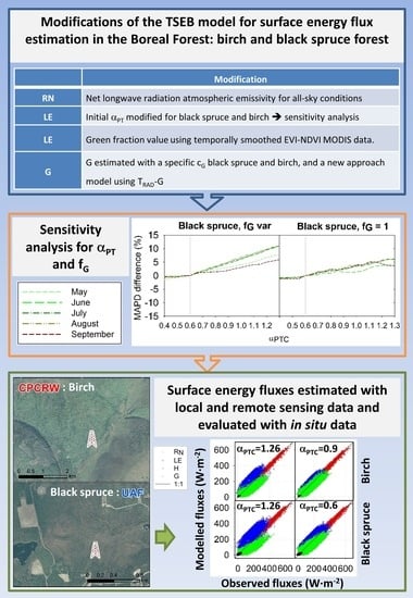
Figure 1. Location of the black spruce (UAF) and the birch (CPCRW) flux towers. Coordinates [km] in UTM-6N Datum NAD-83.
Remotesensing 12 04108 g001
Figure 2. Comparison of modelled vs. measured 30-min fluxes using an initial TSEB αPTC value of 1.26 at both settings, 0.6 for black spruce setting, and 0.9 for birch setting. Perfect agreement is represented by the 1:1 line.
Remotesensing 12 04108 g002
Figure 3. Seasonal behavior of LAI (dashed line) and fG (solid line) from 2012 to 2016 for the study period (May to September) at black spruce (UAF, top panel), and birch (CPCRW, bottom panel) flux towers. Black crosses are the LAI in-situ estimates.
Remotesensing 12 04108 g003
Figure 4. Comparison of modelled vs. observed 30-min fluxes monthly aggregated using an initial TSEB αPTC value 0.6 for black spruce setting and 0.9 for birch setting and G estimated by the G-TRAD relationship. Perfect agreement is represented by the 1:1 line.
Remotesensing 12 04108 g004
Figure 5. Vapour pressure deficit (VPD, in kPa) and αPTS daytime monthly averages from May to September for the 2012–2016 period computed using the flux tower data at birch and black spruce flux towers.
Remotesensing 12 04108 g005
Figure 6. Sensitivity analysis on LE estimation running TSEB with αPTC increasing in value at an interval of 0.05 from 0.4 to 1.3 for both black spruce and birch, respectively, with (a) a variable fG derived from the EVI and NDVI ratio and (b) a fG = 1. RMSE results were monthly averaged from May to September for the 2012–2016 period. Vertical grey lines are the reference adjusted αPTC values used in TSEB to model LE for black spruce and birch.
Remotesensing 12 04108 g006
Figure 7. Error percentage (MAPD) differences on LE estimation running TSEB with αPTC value increases at 0.05 intervals from 0.4 to 1.3 for both black spruce and birch, respectively, with (a) a variable fG derived from the EVI and NDVI ratio and (b) a fG = 1. Results were monthly averaged from May to September for the 2012–2016 period. Error percentage differences were obtained by subtracting a MAPD value from LE estimated at each 0.05 interval in the value of αPTC from 0.4 to 1.3 from the reference αPTC value of 0.6 and 0.9 for black spruce and birch, respectively. Vertical grey lines are the reference adjusted αPTC values used in TSEB to model LE for black spruce and birch.
Remotesensing 12 04108 g007
Figure 8. Modelled vs. observed surface fluxes comparison at satellite pass using αPTC of 0.6 and 0.9 for black spruce and birch settings, respectively, G estimated by the G-TRAD approach and TRAD from MODIS data. Perfect agreement is represented by the 1:1 line.
Remotesensing 12 04108 g008
Figure 9. Comparison of remote sensing estimates of TRAD vs. at-satellite pass observed measurements of TRAD at black spruce and birch flux towers. Perfect agreement is represented by the 1:1 line.
Remotesensing 12 04108 g009
Table 1. TSEB model modifications for the boreal forest.
Surface Energy Flux.TSEB Original FormulationModificationEquation
RNNet longwave radiation atmospheric emissivity for clear-sky conditionsNet longwave radiation atmospheric emissivity for all-sky conditionsEquation (5)
LEInitial αPT = 1.26 for all land coversInitial αPT values for black spruce and birch forests of 0.6 and 0.9, respectively. Equation (12)
LEGreen cover fraction, fG, held constantValue of fG is varied using temporally smoothed EVI-NDVI MODIS data. Equation (12)
GG estimated using cG = 0.3G estimated with a specific cG value of 0.07 for black spruce and birch, and a new proposed model using TRAD-G relationship, cGTEquations (14) and (18)
Table 2. Results of the model agreement and error estimation compared to observed flux tower data using an initial TSEB αPTC value of 1.26 at both settings, 0.6 for black spruce setting, and 0.9 for birch setting. n is the number of 30-min periods selected. Error estimators (RMSE, mean absolute difference (MAD), MBE) are in W·m−2 while MAPD is in %. G was modelled using cGT in Equation (18) applied to Equation (14). X are the mean values for the estimated energy balance components in W·m−2.
Black Spruce|αPTC = 1.26 Black Spruce|αPTC = 0.6
XR2RMSEMBEMADMAPDn XR2RMSEMBEMADMAPDn
RN3080.981801454067RN3080.981801454067
LE1830.7664475339LE1560.7741203324
H1140.8165−495332H1400.8442−233320
G100.4751444G100.4751444
Birch|αPTC = 1.26 Birch|αPTC = 0.9
XR2RMSEMBEMADMAPDn XR2RMSEMBEMADMAPDn
RN3390.982241855528RN3390.982241855528
zLE2160.7477566239LE1840.7649243924
H1050.7971−525636H1360.846−213623
G140.657−3347G140.657−3347
Table 3. Monthly results of the model agreement and error estimation compared to observed flux tower data at the black spruce setting using an initial TSEB αPTC value of 0.6. n is the number of 30-min periods selected. Error estimators (RMSE, MBE, MAD) are in W·m−2 while MAPD is in %.
RNLE
nR2RMSEMBEMADMAPDR2RMSEMBEMADMAPD
May8870.9820−91550.8042213426
June9960.9818−41440.8138153020
July10980.9817−11340.7938153021
August8520.981851450.7544263528
September2340.951721360.7455434845
HG
nR2RMSEMBEMADMAPDR2RMSEMBEMADMAPD
May8870.8449−3640250.10756163
June9960.8841−2132190.3862553
July10980.8636−1328190.725−3424
August8520.8239−2031250.684−1326
September2340.7055−4246460.4142357
Table 4. Monthly results of the model agreement and error estimation compared to observed flux tower data at the birch setting using an initial TSEB αPTC value of 0.9. n is the number of 30-min periods selected. Error estimators (RMSE, MBE, MAD) are in W·m−2 while MAPD is in %.
RNLE
nR2RMSEMBEMADMAPDR2RMSEMBEMADMAPD
May12730.9821−71650.7062455243
June14090.982211850.7846203619
July12270.981931650.764293316
August10630.982191760.7743173419
September5560.95251320100.6869585962
HG
nR2RMSEMBEMADMAPDR2RMSEMBEMADMAPD
May12730.8565−5356340.4091754
June14090.8740−1431220.767−5628
July12270.8436−528230.795−2421
August10630.7936−1028280.7762537
September5560.7160−5051500.70866167
Table 5. Model agreement and error estimation using Terra/Aqua MODIS surface temperature as TRAD and an initial TSEB αPTC value 0.6 and 0.9 for black spruce and birch settings, respectively. Error estimators (RMSE, MBE, MAD) are in W·m−2 while MAPD is in %. X are the mean values for the estimated energy balance components in W·m−2
Black Spruce|αPT = 0.6 Birch|αPT = 0.9
XR2RMSEMBEMADMAPDn XR2RMSEMBEMADMAPDn
RN4690.981710143183RN4660.992519215261
LE2770.7466576232LE3070.7860515825
H1800.7259−495420H1430.7648−314218
G120.3252446G150.716−2735
Publisher’s Note: MDPI stays neutral with regard to jurisdictional claims in published maps and institutional affiliations.

