A Spectra Classification Methodology of Hyperspectral Infrared Images for Near Real-Time Estimation of the SO2 Emission Flux from Mount Etna with LARA Radiative Transfer Retrieval Model

 ,
,  ,
, 
Abstract
1. Introduction
2. Materials and Methods
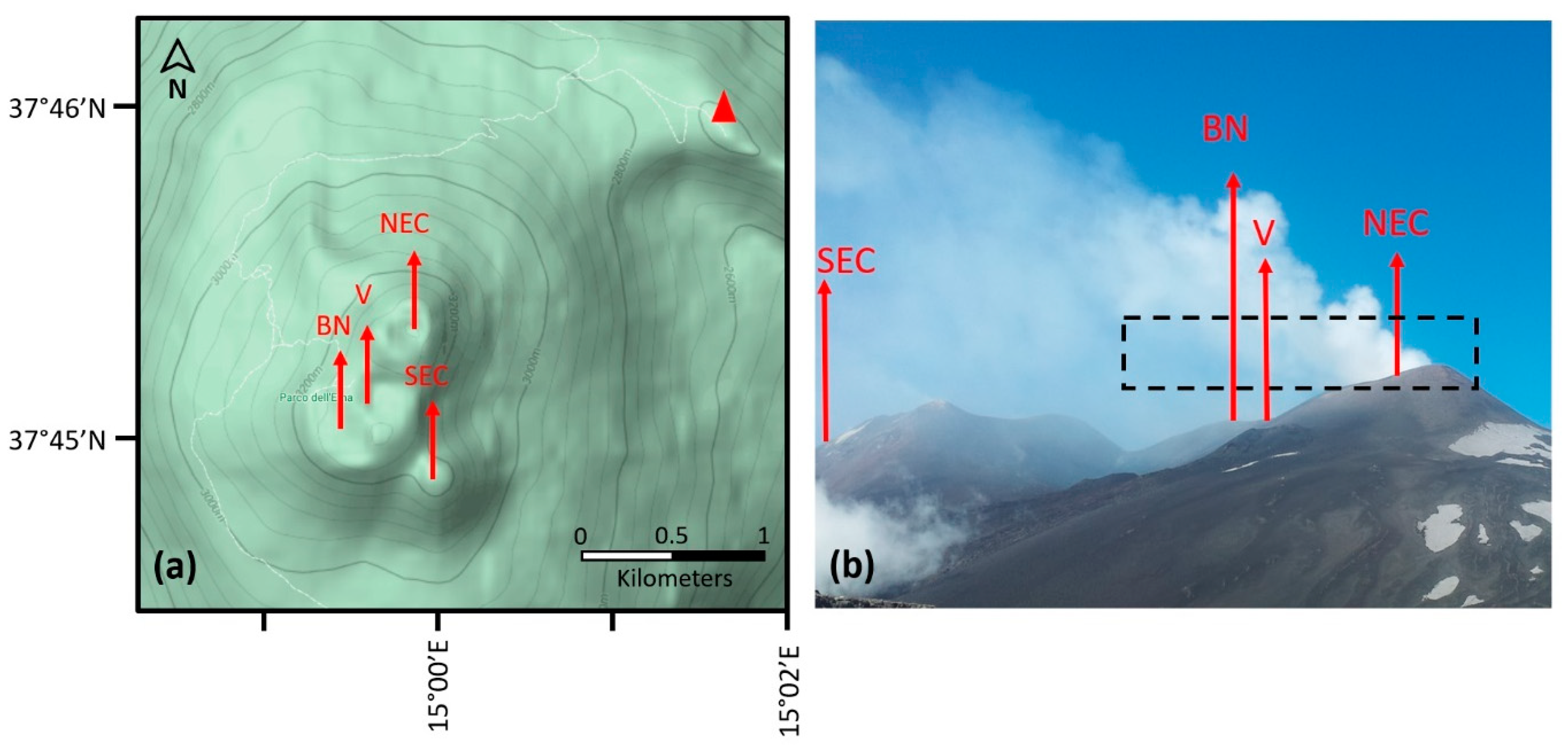
2.1. Overview of the Data
2.2. Retrieval Model: LARA
2.3. Massive Retrieval Methodology
2.3.1. Hyper-Cam Spectral Band Analysis
2.3.2. O3 Emission Region: Spectral “Band 1”
2.3.3. SO2 Emission Region: Spectral “Band 2”
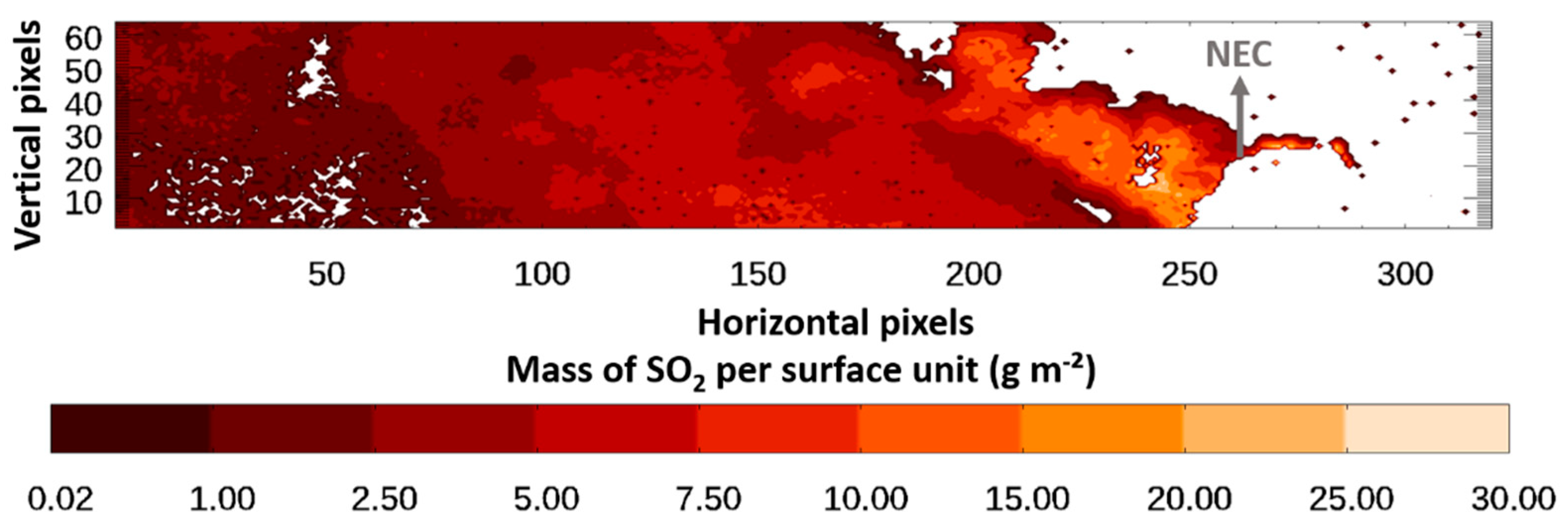
2.4. SO2 Emission Flux Estimation
2.4.1. Plume Transport Speed
2.4.2. Box Method for the Emission Flux Estimation
3. Results
3.1. Training Dataset
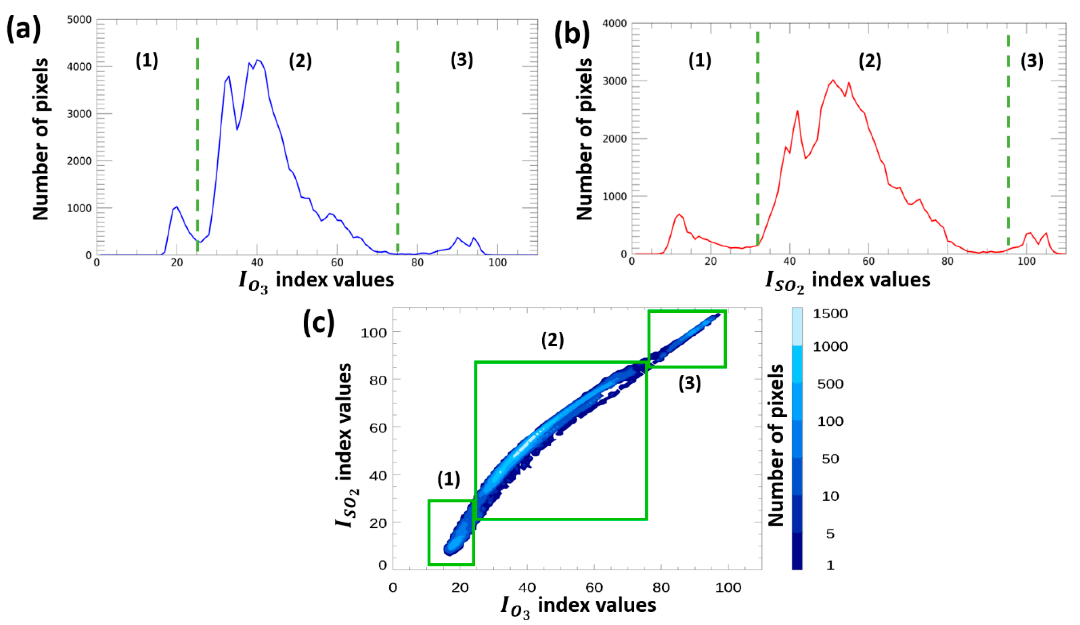
3.1.1. Interval Width for Index
3.1.2. Interval Width for Index
3.1.3. Class Weight Distribution
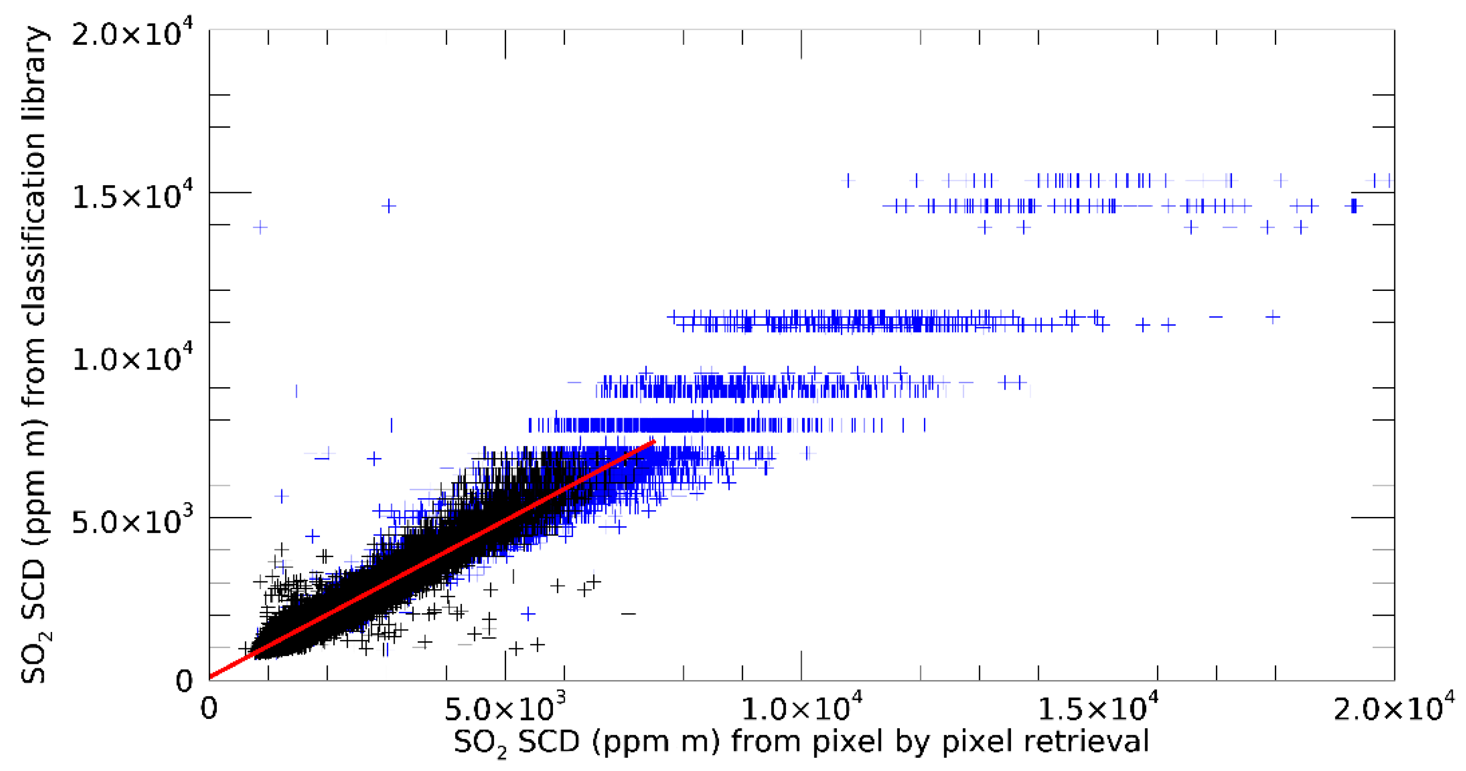
3.1.4. Analysis of the Classification Accuracy
3.2. Tested Dataset
3.3. SO2 Emission Flux
4. Discussion
5. Conclusions
Supplementary Materials
Author Contributions
Funding
Acknowledgments
Conflicts of Interest
References
- Doocy, S.; Daniels, A.; Dooling, S.; Gorokhovich, Y. The human impact of volcanoes: A historical review of events 1900-2009 and systematic literature review. PLoS Curr. 2013, 5. [Google Scholar] [CrossRef] [PubMed]
- Allard, P.; Behncke, B.; D’Amico, S.; Neri, M.; Gambino, S. Mount Etna 1993–2005: Anatomy of an evolving eruptive cycle. Earth-Sci. Rev. 2006, 78, 85–114. [Google Scholar] [CrossRef]
- Caltabiano, T.; Romano, R.; Budetta, G. SO2 flux measurements at Mount Etna (Sicily). J. Geophys. Res. 1994, 99, 12809–12819. [Google Scholar] [CrossRef]
- Oppenheimer, C. Volcanic Degassing. In Treatise on Geochemistry; Holland, H.D., Turekian, K.K., Eds.; Elsevier Inc.: Amsterdam, The Netherlands, 2003; pp. 123–166. [Google Scholar] [CrossRef]
- Aiuppa, A.; Moretti, R.; Federico, C.; Giudice, G.; Gurrieri, S.; Liuzzo, M.; Papale, P.; Shinohara, H.; Valenza, M. Forecasting Etna eruptions by real-time observation of volcanic gas composition. Geology 2007, 35, 1115–1118. [Google Scholar] [CrossRef]
- Sparks, R.S.J. Forecasting volcanic eruptions. Earth Planet. Sci. Lett. 2003, 210, 1–15. [Google Scholar] [CrossRef]
- D’Aleo, R.; Bitetto, M.; Delle Donne, D.; Coltelli, M.; Coppola, D.; McCormick Kilbride, B.; Pecora, E.; Ripepe, M.; Salem, L.C.; Tamburello, G.; et al. Understanding the SO2 degassing budget of Mt Etna’s paroxysms: First clues from the December 2015 sequence. Front. Earth Sci. 2019, 6. [Google Scholar] [CrossRef]
- Delle Donne, D.; Aiuppa, A.; Bitetto, M.; D’Aleo, R.; Coltelli, M.; Coppola, D.; Pecora, E.; Ripepe, M.; Tamburello, G. Changes in SO2 flux regime at Mt. Etna captured by automatically processed ultraviolet camera data. Remote Sens. 2019, 11, 1201. [Google Scholar] [CrossRef]
- Burton, M.; Allard, P.; Muré, F.; La Spina, A. Magmatic gas composition reveals the source depth of slug-driven strombolian explosive activity. Science 2007, 317, 227–230. [Google Scholar] [CrossRef]
- Vergniolle, S.; Jaupart, C. Dynamics of degassing at Kilauea Volcano, Hawaii. J. Geophys. Res. 1990, 95, 2793–2809. [Google Scholar] [CrossRef]
- Robock, A. Volcanic eruptions and climate. Rev. Geophys. 2000, 38, 191–219. [Google Scholar] [CrossRef]
- Hansell, A.; Oppenheimer, C. Health Hazards from Volcanic Gases: A Systematic Literature Review. Arch. Environ. Health Int. J. 2004, 59, 628–639. [Google Scholar] [CrossRef] [PubMed]
- Williams-Jones, G.; Rymer, H. Hazards of Volcanic Gases. In The Encyclopedia of Volcanoes, 2nd ed.; Sigurdsson, H., Houghton, B., Rymer, H., Stix, J., McNutt, S., Eds.; Elsevier Inc.: Amsterdam, The Netherlands, 2015; pp. 985–992. [Google Scholar] [CrossRef]
- Prata, F.; Bluth, G.; Werner, C.; Realmunto, V.; Carn, S.; Watson, M. Remote sensing of gas emissions from volcanoes. In Monitoring Volcanoes in the North Pacific: Observations from Space; Dean, K.G., Dehn, J., Eds.; Springer: Berlin/Heidelberg, Germany, 2015; pp. 145–186. [Google Scholar] [CrossRef]
- Allard, P. Endogenous magma degassing and storage at Mount Etna. Geophys. Res. Lett. 1997, 24, 2219–2222. [Google Scholar] [CrossRef]
- Carn, S.A.; Krueger, A.J.; Arellano, S.; Krotkov, N.A.; Yang, K. Daily monitoring of Ecuadorian volcanic degassing from space. J. Volcanol. Geotherm. Res. 2008, 176, 141–150. [Google Scholar] [CrossRef]
- Carn, S.A.; Clarisse, L.; Prata, A.J. Multi-decadal satellite measurements of global volcanic degassing. J. Volcanol. Geotherm. Res. 2016, 311, 99–134. [Google Scholar] [CrossRef]
- Gouhier, M.; Paris, R. SO2 and tephra emissions during the December 22, 2018 Anak Krakatau eruption. Volcanica 2019, 2, 91–103. [Google Scholar] [CrossRef]
- Theys, N.; Hedelt, P.; De Smedt, I.; Lerot, C.; Yu, H.; Vlietinck, J.; Pedergnana, M.; Arellano, S.; Galle, B.; Fernandez, D.; et al. Global monitoring of volcanic SO2 degassing with unprecedented resolution from TROPOMI onboard Sentinel-5 Precursor. Sci. Rep. 2019, 9, 2643. [Google Scholar] [CrossRef]
- Watson, I.M.; Realmunto, V.J.; Rose, W.I.; Prata, A.J.; Bluth, G.J.S.; Gu, Y.; Bader, C.E.; Yu, T. Thermal infrared remote sensing of volcanic emissions using the moderate resolution imaging spectroradiometer. J. Volcanol. Geotherm. Res. 2004, 135, 75–89. [Google Scholar] [CrossRef]
- Prata, A.J.; Kerkmann, J. Simultaneous retrieval of volcanic ash and SO2 using MSG-SEVIRI measurements. Geophys. Res. Lett. 2007, 35, L05813:1–L05813:6. [Google Scholar] [CrossRef]
- Karagulian, F.; Clarisse, L.; Clerbaux, C.; Prata, A.J.; Hurtmans, D.; Coheur, P.F. Detection of volcanic SO2, ash, and H2SO4 using the Infrared Atmospheric Sounding Interferometer (IASI). J. Geophys. Res. Atmos. 2010, 115, D00L02:1–D00L02:10. [Google Scholar] [CrossRef]
- Carn, S.A.; Strow, L.L.; de Souza-Machado, S.; Edmonds, Y.; Hannon, S. Quantifying tropospheric volcanic emissions with AIRS: The 2002 eruption of Mt. Etna (Italy). Geophys. Res. Lett. 2005, 32, L02301:1–L02301:5. [Google Scholar] [CrossRef]
- Mori, T.; Burton, M. The SO2 camera: A simple, fast and cheap method for ground-based imaging of SO2 in volcanic plumes. Geophys. Res. Lett. 2006, 33, L24804:1–L24804:5. [Google Scholar] [CrossRef]
- Galle, B.; Oppenheimer, C.; Geyer, A.; McGonigle, A.J.S.; Edmonds, M.; Horrokcs, L. A miniaturised ultraviolet spectrometer for remote sensing of SO2 fluxes: A new tool for volcano surveillance. J. Volcanol. Geotherm. Res. 2003, 119, 241–254. [Google Scholar] [CrossRef]
- Edmonds, M.; Herd, R.A.; Galle, B.; Oppenheimer, C.M. Automated, high time-resolution measurements of SO2 flux at Soufrière Hills Volcano, Montserrat. Bull. Volcanol. 2003, 65, 578–586. [Google Scholar] [CrossRef]
- Prata, A.J.; Bernardo, C. Retrieval of sulfur dioxide from a ground-based thermal infrared imaging camera. Atmos. Meas. Tech. 2014, 7, 2807–2828. [Google Scholar] [CrossRef]
- Merucci, L.; Burton, M.; Corradini, S.; Salerno, G.G. Reconstruction of SO2 flux emission chronology from space-based measurements. J. Volcanol. Geotherm. Res. 2011, 206, 80–87. [Google Scholar] [CrossRef]
- Galle, B.; Johansson, M.; Rivera, C.; Zhang, Y.; Kihlman, M.; Kern, C.; Lehmann, T.; Platt, U.; Arellano, S.; Hidalgo, S. Network for Observation of Volcanic and Atmospheric Change (NOVAC)—A global network for volcanic gas monitoring: Network layout and instrument description. J. Geophys. Res. Atmos. 2010, 115, D05304:1–D05304:19. [Google Scholar] [CrossRef]
- Salerno, G.G.; Burton, M.R.; Oppenheimer, C.; Caltabiano, T.; Randazzo, D.; Bruno, N.; Longo, V. Three-years of SO2 flux measurements of Mt. Etna using an automated UV scanner array: Comparison with conventional traverses and uncertainties in flux retrieval. J. Volcanol. Geotherm. Res. 2009, 183, 76–83. [Google Scholar] [CrossRef]
- Queißer, M.; Burton, M.; Theys, N.; Pardini, F.; Salerno, G.; Caltabiano, T.; Varnam, M.; Esse, B.; Kazahaya, R. TROPOMI enables high resolution SO 2 flux observations from Mt. Etna, Italy, and beyond. Sci. Rep. 2019, 9, 957. [Google Scholar] [CrossRef]
- D’Aleo, R.; Bitetto, M.; Donne, D.D.; Tamburello, G.; Battaglia, A.; Coltelli, M.; Patanè, D.; Prestifilippo, M.; Sciotto, M.; Aiuppa, A. Spatially resolved SO2 flux emissions from Mt Etna. Geophys. Res. Lett. 2016, 43, 7511–7519. [Google Scholar] [CrossRef]
- Smekens, J.F.; Gouhier, M. Observation of SO2 degassing at Stromboli volcano using a hyperspectral thermal infrared imager. J. Volcanol. Geotherm. Res. 2018. [Google Scholar] [CrossRef]
- Huret, N.; Segonne, C.; Payan, S.; Salerno, G.; Catoire, V.; Ferrec, Y.; Roberts, T.; Pola Fossi, A.; Rodriguez, D.; Croizé, L.; et al. Infrared Hyperspectral and Ultraviolet Remote Measurements of Volcanic Gas Plume at MT Etna during IMAGETNA Campaign. Remote Sens. 2019, 11, 1175. [Google Scholar] [CrossRef]
- Wright, R.; Lucey, P.; Crites, S.; Horton, K.; Wood, M.; Garbeil, H. BBM/EM design of the thermal hyperspectral imager: An instrument for remote sensing of earth’s surface, atmosphere and ocean, from a microsatellite platform. Acta Astronaut. 2013, 87, 182–192. [Google Scholar] [CrossRef]
- Clark, M.L.; Roberts, D.A.; Clark, D.B. Hyperspectral discrimination of tropical rain forest tree species at leaf to crown scales. Remote Sens. Environ. 2005, 96, 375–398. [Google Scholar] [CrossRef]
- Briottet, X.; Boucher, Y.; Dimmeler, A.; Malaplate, A.; Cini, A.; Diani, M.; Bekman, H.; Schwering, P.; Skauli, T.; Kasen, I.; et al. Military applications of hyperspectral imagery. In Proceedings of the Targets and Backgrounds XII: Characterization and Representation; International Society for Optics and Photonics, Defense and Security Symposium, Orlando, FL, USA, 17–21 April 2006; Volume 6239, p. 62390B. [Google Scholar]
- Paoletti, M.E.; Haut, J.M.; Plaza, J.; Plaza, A. Deep learning classifiers for hyperspectral imaging: A review. ISPRS J. Photogramm. Remote Sens. 2019, 158, 279–317. [Google Scholar] [CrossRef]
- Lu, D.; Weng, Q. A survey of image classification methods and techniques for improving classification performance. Int. J. Remote Sens. 2007, 28, 823–870. [Google Scholar] [CrossRef]
- Van Damme, M.; Whitburn, S.; Clarisse, L.; Clerbaux, C.; Hurtmans, D.; Coheur, P.-F. Version 2 of the IASI NH3 neural network retrieval algorithm: Near-real-time and reanalysed datasets. Atmos. Meas. Tech. 2017, 10, 4905–4914. [Google Scholar] [CrossRef]
- Lagueux, P.; Farley, V.; Chamberland, M.; Villemaire, A.; Turcotte, C.; Puckrin, E. Design and Performance of the Hyper-Cam, an Infrared Hyperspectral Imaging Sensor. Available online: https://www.semanticscholar.org/paper/Design-and-Performance-of-the-Hyper-Cam%2C-an-Imaging-Lagueux-Farley/2f7590496d218177bd059fe6bbab98ad69afc36e (accessed on 14 December 2020).
- Calvari, S.; Coltelli, M.; Müller, W.; Pompilio, M.; Scribano, V. Eruptive history of South-Eastern crater of Mount Etna, from 1971 to 1994. Acta Vulcanol. 1994, 5, 11–14. [Google Scholar]
- Rodgers, C.D. Inverse Methods for Atmospheric Sounding: Theory and Practice; Atmospheric, Oceanic and Planetary Physics—Volume 2; World Scientific: Singapore, 2000. [Google Scholar]
- Payan, S.; Camy-Peyret, C.; Jeseck, P.; Hawat, T.; Durry, G.; Lefèvre, F. First direct simultaneous HCl and ClONO2 profile measurements in the Arctic Vortex. Geophys. Res. Lett. 1998, 25, 2663–2666. [Google Scholar] [CrossRef]
- Payan, S.; Camy-Peyret, C.; Bureau, J. Comparison of Retrieved L2 Products from Four Successive Versions of L1B Spectra in the Thermal Infrared Band of TANSO-FTS over the Arctic Ocean. Remote Sens. 2017, 9, 1167. [Google Scholar] [CrossRef]
- Butz, A.; Bösch, H.; Camy-Peyret, C.; Dorf, M.; Engel, A.; Payan, S.; Pfeilsticker, K. Observational constraints on the kinetics of the ClO-BrO and ClO-ClO ozone loss cycles in the Arctic winter stratosphere. Geophys. Res. Lett. 2007, 34, L05801:1–L05801:5. [Google Scholar] [CrossRef]
- Payan, S.; Camy-Peyret, C.; Oelhaf, H.; Wetzel, G.; Maucher, G.; Keim, C.; Pirre, M.; Huret, N.; Engel, A.; Volk, M.C.; et al. Validation of version-4.61 methane and nitrous oxide observed by MIPAS. Atmos. Chem. Phys. 2009, 9, 413–442. [Google Scholar] [CrossRef]
- Keim, C.; Eremenko, M.; Orphal, J.; Dufour, G.; Flaud, J.-M.; Höpfner, M.; Boynard, A.; Clerbaux, C.; Payan, S.; Coheur, P.-F.; et al. Tropospheric ozone from IASI: Comparison of different inversion algorithms and validation with ozone sondes in the northern middle latitudes. Atmos. Chem. Phys. 2009, 9, 9329–9347. [Google Scholar] [CrossRef]
- Clough, S.A.; Shephard, M.W.; Mlawer, E.J.; Delamere, J.S.; Iacono, M.J.; Cady-Pereira, K.; Boukabara, S.; Brown, P.D. Atmospheric radiative transfer modeling: A summary of the AER codes. J. Quant. Spectrosc. Radiat. Transf. 2005, 91, 233–244. [Google Scholar] [CrossRef]
- Aiuppa, A.; Fiorani, L.; Santoro, S.; Parracino, S.; Nuvoli, M.; Chiodini, G.; Minopoli, C.; Tamburello, G. New ground-based lidar enables volcanic CO2 flux measurements. Sci. Rep. 2015, 5, 13614. [Google Scholar] [CrossRef] [PubMed]
- Theys, N.; Campion, R.; Clarisse, L.; Brenot, H.; van Gent, J.; Dils, B.; Corradini, S.; Merucci, L.; Coheur, P.-F.; Van Roozendael, M.; et al. Volcanic SO2 fluxes derived from satellite data: A survey using OMI, GOME-2, IASI and MODIS. Atmos. Chem. Phys. 2013, 13, 5945–5968. [Google Scholar] [CrossRef]
- McGonigle, A.J.S.; Delmelle, P.; Oppenheimer, C.; Tsanev, V.I.; Delfosse, T.; Williams-Jones, G.; Horton, K.; Mather, T.A. SO2 depletion in tropospheric volcanic plumes. Geophys. Res. Lett. 2004, 31, L13201:1–L13201:4. [Google Scholar] [CrossRef]
- Aiuppa, A.; Giudice, G.; Gurrieri, S.; Liuzzo, M.; Burton, M.; Caltabiano, T.; McGonigle, A.J.S.; Salerno, G.; Shinohara, H.; Valenza, M. Total volatile flux from Mount Etna. Geophys. Res. Lett. 2008, 35, L24302:1–L24302:5. [Google Scholar] [CrossRef]
- La Spina, A.; Burton, M.; Salerno, G.G. Unravelling the processes controlling gas emissions from the central and northeast craters of Mt. Etna. J. Volcanol. Geotherm. Res. 2010, 198, 368–376. [Google Scholar] [CrossRef]
- Gliß, J.; Stebel, K.; Kylling, A.; Sudbø, A. Improved optical flow velocity analysis in SO2 camera images of volcanic plumes—Implications for emission-rate retrievals investigated at Mt Etna, Italy and Guallatiri, Chile. Atmos. Meas. Tech. 2018, 11, 781–801. [Google Scholar] [CrossRef]
- Oppenheimer, C.; Tsanev, V.I.; Braban, C.F.; Cox, R.A.; Adams, J.W.; Aiuppa, A.; Bobrowski, N.; Delmelle, P.; Barclay, J.; McGonigle, A.J.S. BrO formation in volcanic plumes. Geochim. Cosmochim. Acta 2006, 70, 2935–2941. [Google Scholar] [CrossRef]
- Gabrieli, A.; Wright, R.; Porter, J.N.; Lucey, P.G.; Honnibal, C. Applications of quantitative thermal infrared hyperspectral imaging (8–14 μm): Measuring volcanic SO2 mass flux and determining plume transport velocity using a single sensor. Bull. Volcanol. 2019, 81. [Google Scholar] [CrossRef]


| # | Date Time | Spectral Resolution (cm−1) | Image Acquisition Time | Number of Images | Total Number of Pixels | Sequence Duration | Broadband IR Image |
|---|---|---|---|---|---|---|---|
| A | 23-06-2015 08:12:45 – 08:22:22 (UTC *) | 2 | 4.595 s | 120 | 2.46 × 10⁶ | 9′37″ |  |
| B | 26-06-2015 08:25:25 – 08:38:50 (UTC) | 2 | 2.547 s | 288 | 5.90 × 10⁶ | 13′25″ |  |
| C | 26-06-2015 07:17:59 – 07:29:02 (UTC) | 4 | 1.274 s | 470 | 9.63 × 10⁶ | 11′03″ |  |
| Tested Ranges (K cm−1) | Percent of Plume Pixels/Classes with Relative Standard Deviation on SO2 SCD < 10% | Number of Classes with a Relative Standard Deviation on SO2 SCD < 10% |
|---|---|---|
| 10 | 47.7/35.1 | 629 |
| 50 | 47.1/29.7 | 133 |
| 100 | 48/30.6 | 78 |
| 500 | 25.9/20.4 | 21 |
| Tested Ranges (K) | Percent of Plume Pixels/Classes with Relative Standard Deviation on SO2 SCD < 10% | Number of Classes with Relative Standard Deviation on SO2 SCD < 10% |
|---|---|---|
| 1 | 48/30.6 | 78 |
| 5 | 14.1/21.7 | 18 |
| 10 | 6.3/14.5 | 9 |
| Sequence # | Classification Time (s/Image) | Number of Classes: In the Plume/Out of Plume Library | Percent of Pixels from Plume Out of the Library |
|---|---|---|---|
| A | 36.7 | 560/109 | 22.5 |
| B | 33.8 | 687/156 | 20.6 |
| C | 15.3 | 754/99 | 15.0 |
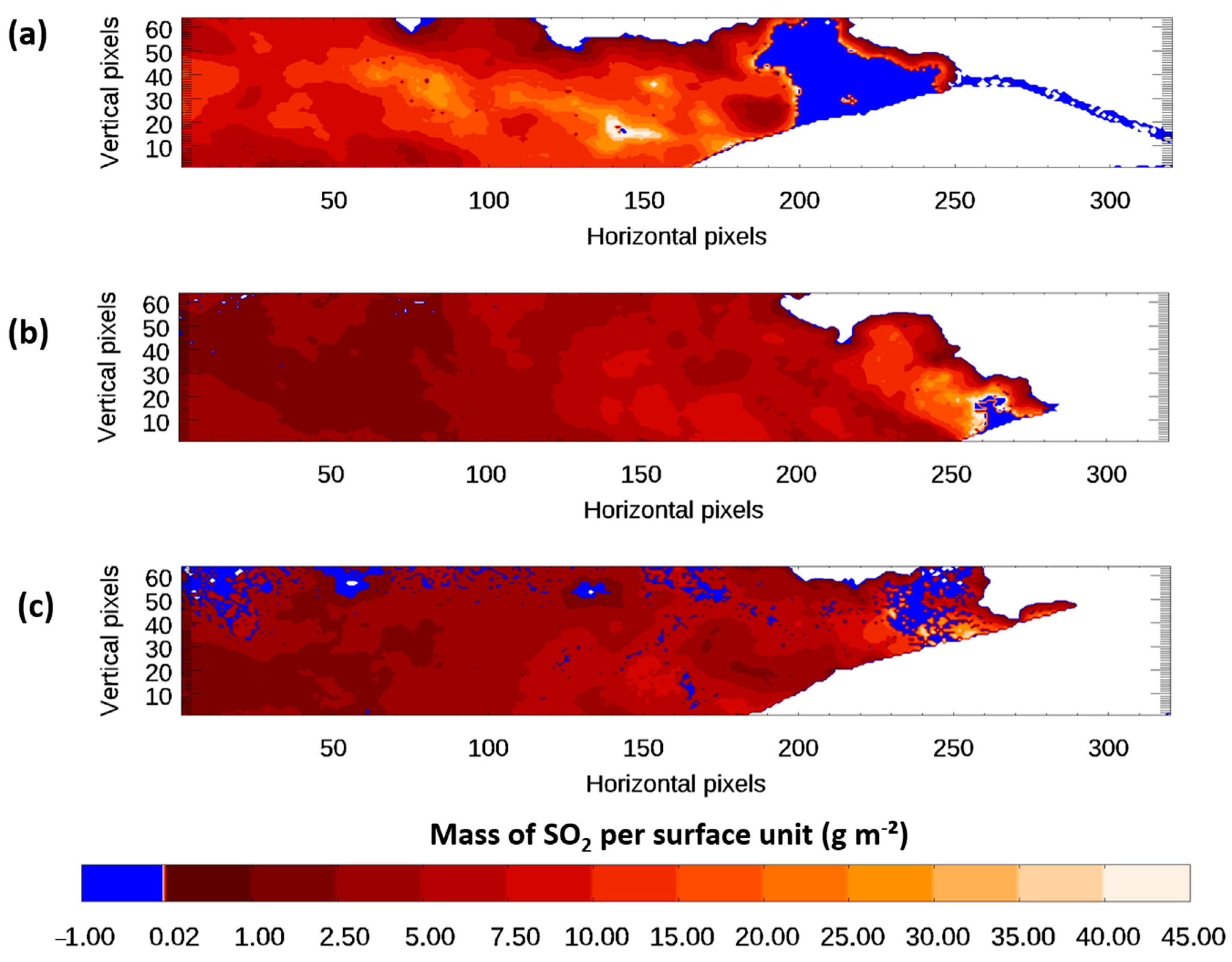
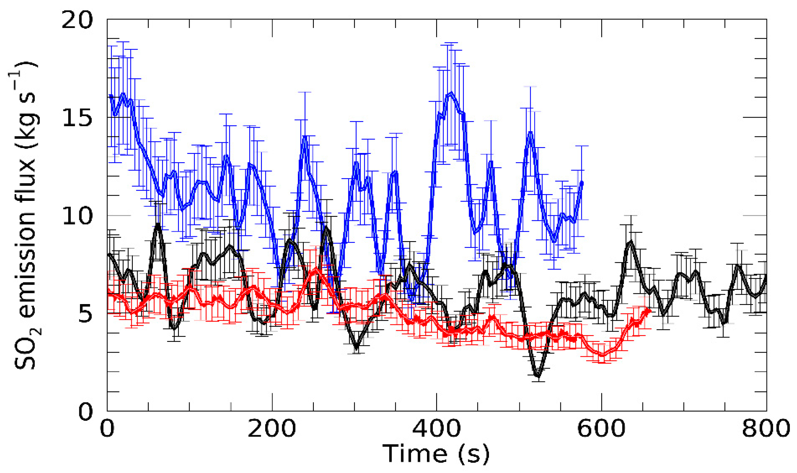
| # | Plume Transport Speed | Average Mass of SO2 Per Surface Unit | Average SO2 Emission Flux | |
|---|---|---|---|---|
| (m s−1) | (g m−2) | (kg s−1) | (t day−1) | |
| A | 5.83 | 10.54 ± 7.76 | 10.87 ± 2.61 | 938.84 ± 225.25 |
| B | 6.66 | 5.34 ± 4.53 | 6.13 ± 1.41 | 529.79 ± 122.13 |
| C | 6.62 | 4.56 ± 2.93 | 4.95 ± 0.98 | 427.51 ± 85.15 |
Publisher’s Note: MDPI stays neutral with regard to jurisdictional claims in published maps and institutional affiliations. |
© 2020 by the authors. Licensee MDPI, Basel, Switzerland. This article is an open access article distributed under the terms and conditions of the Creative Commons Attribution (CC BY) license (http://creativecommons.org/licenses/by/4.0/).
Share and Cite
Segonne, C.; Huret, N.; Payan, S.; Gouhier, M.; Catoire, V. A Spectra Classification Methodology of Hyperspectral Infrared Images for Near Real-Time Estimation of the SO2 Emission Flux from Mount Etna with LARA Radiative Transfer Retrieval Model. Remote Sens. 2020, 12, 4107. https://doi.org/10.3390/rs12244107
Segonne C, Huret N, Payan S, Gouhier M, Catoire V. A Spectra Classification Methodology of Hyperspectral Infrared Images for Near Real-Time Estimation of the SO2 Emission Flux from Mount Etna with LARA Radiative Transfer Retrieval Model. Remote Sensing. 2020; 12(24):4107. https://doi.org/10.3390/rs12244107
Chicago/Turabian StyleSegonne, Charlotte, Nathalie Huret, Sébastien Payan, Mathieu Gouhier, and Valéry Catoire. 2020. "A Spectra Classification Methodology of Hyperspectral Infrared Images for Near Real-Time Estimation of the SO2 Emission Flux from Mount Etna with LARA Radiative Transfer Retrieval Model" Remote Sensing 12, no. 24: 4107. https://doi.org/10.3390/rs12244107
APA StyleSegonne, C., Huret, N., Payan, S., Gouhier, M., & Catoire, V. (2020). A Spectra Classification Methodology of Hyperspectral Infrared Images for Near Real-Time Estimation of the SO2 Emission Flux from Mount Etna with LARA Radiative Transfer Retrieval Model. Remote Sensing, 12(24), 4107. https://doi.org/10.3390/rs12244107