Monitoring of Sugarcane Harvest in Brazil Based on Optical and SAR Data

Abstract

The algorithms for determining sugarcane harvest dates are proposed; the algorithms allow the ability to monitor large areas and are based on the publicly available Synthetic Aperture Radar (SAR) and optical satellite data. Algorithm 1 uses the NDVI (Normalized Difference Vegetation Index) time series derived from Sentinel-2 data. Sharp and continuous decrease in the NDVI values is the main sign of sugarcane harvest. The NDVI time series allows the ability to determine most harvest dates. The best estimates of the sugarcane areas harvested per month have been obtained from March to August 2018 when cloudy pixel percentage is less than 45% of the image area. Algorithm 2 of the harvest monitoring uses the coherence time series derived from Sentinel-1 Single Look Complex (SLC) images and optical satellite data. Low coherence, demonstrating sharp growth upon the harvest completion, corresponds to the harvest period. The NDVI time series trends were used to refine the algorithm. It is supposed that the descending NDVI trend corresponds to harvest. The algorithms were used to identify the harvest dates and calculate the harvested areas of the reference sample of 574 sugarcane parcels with a total area of 3745 ha in the state of São Paulo, Brazil. The harvested areas identified by visual interpretation coincide with the optical-data algorithm (algorithm 1) by 97%; the coincidence with the algorithm based on SAR and optical data (algorithm 2) is 90%. The main practical applications of the algorithms are harvest monitoring and identification of the harvested fields to estimate the harvested area.

1. Introduction

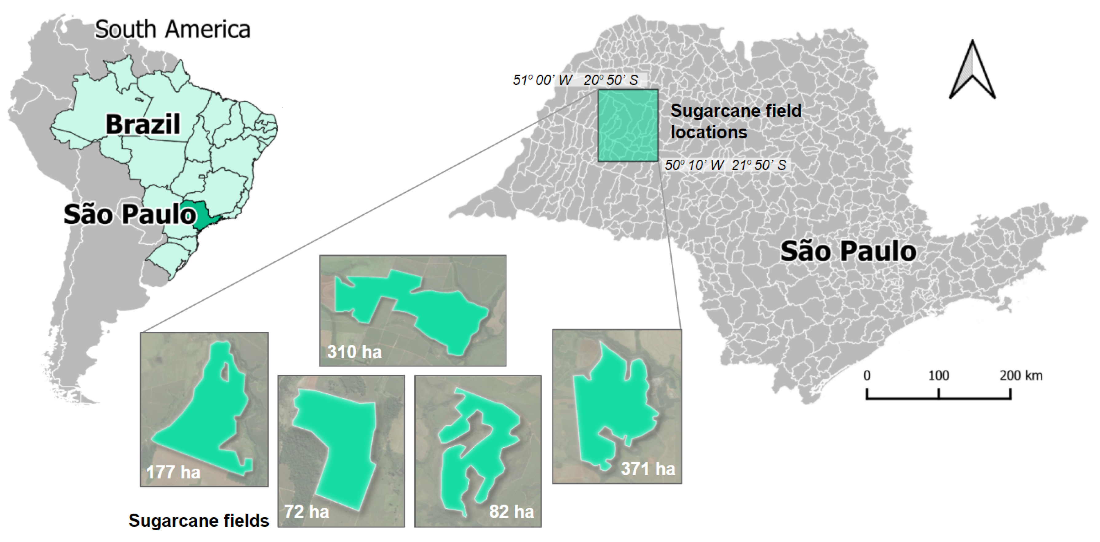
Sugarcane is the key industrial crop for Brazil and a number of other countries (e.g., India, China, Thailand, etc.) [1]. Monitoring of sugarcane harvest is important to schedule and optimize logistic operations as well as forecast the crop productivity. The latter is applied to forecast the production indicators of sugar industry enterprises, biofuel (ethanol), etc. [2,3,4,5,6]. In Brazil, 60% of the sugarcane fields are located in the state of São Paulo [7]. Recently, Brazil has been demonstrating the rapid transition from the low-productive, costly, and environmentally unfriendly (due to preliminary burning of sugarcane leaves) technologies of manual harvest to mechanized harvest technologies (harvest without burning—green harvest) [5,8]. That makes it possible to accelerate considerably the rate of operations and harvest throughout a year including the rainy season. Along with the growing Earth population and increasing rates of global economic development, the need for sugar industry products is rising as well. That requires the development and application of innovative technologies for sugarcane growing and harvest, and as a result—the implementation of a global harvest monitoring to evaluate the production output and to control certain changes in the fields.

Ground-based harvest monitoring is possible by installing the navigation equipment and receiving GPS data from harvesters, tractors, and semi-trucks [9]. The equipment transmits in real-time mode the signal about the machinery location (latitude and longitude) to a remote receiving station. An operator transforms the geographical coordinates into a spatial data file for their visualization in a GIS viewer and evaluation of the harvested parcel area. The methods based on the processing of digital mosaics of optical and SAR (Synthetic Aperture Radar) images of sub-meter spatial resolution, obtained from the Unmanned Aerial Vehicle (UAV), allow the ability to construct a detailed map of plants within the territory under study with an area of several hectares [10,11]. Such approaches are efficient on a field and farming enterprise level; however, they require considerable costs while monitoring on regional, state or the whole country level. The solution here is to use the global satellite monitoring data with a spatial resolution compatible with the size of sugarcane fields [12].

To estimate sugarcane vegetation conditions and evaluate the content of nitrogen, moisture, and salts in the plant stalks, recent studies of the modern authors often involve different spectral indices, such as NDVI (Normalised Difference Vegetation Index) [13], RVI (Ratio Vegetation Index) [14], EVI (Enhanced Vegetation Index) [15], NDWI (Normalized Difference Water Index) [16]. The studies also pay much attention to optical remote sensing of the crop residue and tillage that is related to the problems of the research [17]. Daughtry et al. [18] highlights considerable differences in spectral reflectance of green vegetation, bare soil, and crop residue. In particular, it is shown that the residue has much higher spectral reflectance in the Short-wave Infra-Red (SWIR) range than the green vegetation or soil. Tuszynska et al. [19] stresses that harvest is characterised by the sharp increase of spectral reflectance in SWIR 1 and SWIR 2 bands of Sentinel-2 satellite. In terms of mechanized harvest, sugarcane is not burnt; thus, during the harvest period, the field has thick green vegetation. When sugarcane is harvested, roots and parts of stalks are left in the soil. Later, new plants will grow from them (ratoon). The residual stalks differ considerably in their spectral characteristics from the plants before harvest. That allows using spectral indices to record the harvest date. For instance, the cane growth and harvest correlates with NDVI, which increases smoothly during the plant growth and decreases sharply after harvest. The complexity is in the fact that in non-irrigated fields, the cane leaves may dry out and differ slightly in the optical images from the harvested stalks. Moreover, along with the development of mechanization technologies, harvest may be carried out during the rainy periods when optical images of the fields are impossible to obtain within the weeks or even months due to the cloudiness. In those cases, SAR images are the only source of information.

Recent papers show the examples of SAR data successful use to find changes in sugarcane state, including the ones related to the harvest. The C-band SAR (Sentinel-1 and Radarsat-2), L-band SAR (ALOS-2), and X-band (TerraSAR-X) data are used successfully to map the state and evaluate the sugarcane productivity [7,10,12]. The possibility to determine the harvest data using SAR images is connected with the fact that SAR images are sensitive to the changing vegetation height and field surface texture due to harvest. The cane harvest may be carried out throughout a year. In addition, several parcels planted and harvested at different periods of time are possible within one cadastral field. Consequently, the main requirements for SAR selection data are as follows: rather high spatial and temporal resolution compatible with the dimensions of field fragments and time interval of harvest [12]. Open access SAR images from Sentinel-1 A/B satellite constellation allow the ability to monitor harvest every 6–12 days with a spatial resolution of up to 10 m. Interaction of radar signal with the surface is determined by the backscattering coefficient (${\sigma }^0$) and coherence—a module of the complex correlation coefficient between two Single Look Complex (SLC) images containing the data on amplitude and phase of radar signal [20]. Harvest is identified by the accompanying abrupt decrease of ${\sigma }^0$ [3]. It is pointed out that along with the cane stalks growth, ${\sigma }^0$ values increase as well. When stalks are cut, ${\sigma }^0$ falls sharply. Changes in ${\sigma }^0$ related to the cutting of an above-ground part of a plant are the most characteristic feature of crop harvest in terms of SAR data [21,22,23]. During that period, coherence is low since SAR-images before and after harvest correlate weakly between each other [24,25]. However, since the SAR-images regularity is several days (6–12 days for Sentinel-1) and mechanized harvest may be carried out during rainy periods, there is a high possibility of false detection of harvest dates due to high ${\sigma }^0$ sensitivity for precipitation at minor and medium incidence angles, especially for seedlings (precipitation provokes ${\sigma }^0$ bursts) [12]. Thus, such an approach requires the available additional data on precipitation within the monitoring parcels that complicate its use. Elimination of precipitation effect is possible, for instance, by averaging of ${\sigma }^0$ data at a grid scale 10 km × 10 km: if the ${\sigma }^0$ burst is observed within all grid cells—it is caused by precipitation; otherwise, it is caused by the crop growing [26]. Precipitation can also be detected by the data from local meteorological services and Global Precipitation Measurement (GPM) data [27]. Baghdadi et al. [12] emphasize that possibility of harvest date determining using the TerraSAR-X data is also influenced by the incidence angle. They claim that the best results of harvest mapping may be obtained with an incidence angle of ${37}^{\circ }$.

The Sentinel-1 SLC C-band SAR data have been used successfully to determine crop harvest dates [24]. However, natural conditions and technologies of sugarcane growing differ considerably from the ones described in [24]. Thus, the algorithm [24] applicability for sugarcane needs additional studies.

Numerous papers deal with the application of segmentation, Machine Learning, and Data Mining methods to estimate the sugarcane state using classification maps [28,29,30,31]. The simplest approaches involve classification of the sugarcane state and stages of its growth (including the harvested areas), i.e., with the use of statistic methods (such as a maximum likelihood estimation) or Object-Based Image Analysis (OBIA) [32]. The ${\sigma }^0$ values in different polarizations as well as polarimetric coefficients can be used as inputs in SAR classification tasks [33]. To single out the sugarcane plantations at different growth stages, one can use regression trees (Classification and Regression Trees—CART), support vector machine classifiers (Polynomial-SVM and RBF-SVM), a random forest classifier (RF), an artificial neural network classifier (ANN), and a decision tree classifier (CART-DT) [29,34]. The Random Forest and XGBoost methods may identify the sugarcane plantations to high precision, including the early growth stages (that indicates indirectly the preceding harvest) [33]. Early identification of the agricultural plantings (including the early sugarcane emerging) is possible from Sentinel-1 time series using such neural network classifiers as convolutional neural networks (CNNs), long short-term memory recurrent neural networks (LSTM RNNs), and gated recurrent unit RNNs (GRU RNNs), etc. [35].

The disadvantage of those methods is in the requirement for the available ground-based training sample that is not always possible in the case of regional and global monitoring. Such methods are sensitive to the composition of reference objects and may need additional retraining while transferring to other parcels of the fields being classified. They are often complicated for their implementation and require considerable computational resources.

The objective of the research is to develop the algorithms for determining the harvesting dates suitable for large sugarcane areas monitoring. The algorithm should provide correct results in the lack of a ground-based training sample and be computationally simple, thereby overcoming the limitations of existing methods. To do that, open-access data from Sentinel-1 and Sentinel-2 were used. There are the following main practical implications of the research results: control of the harvesting operations and determination of the harvested fields to estimate the harvested crop.

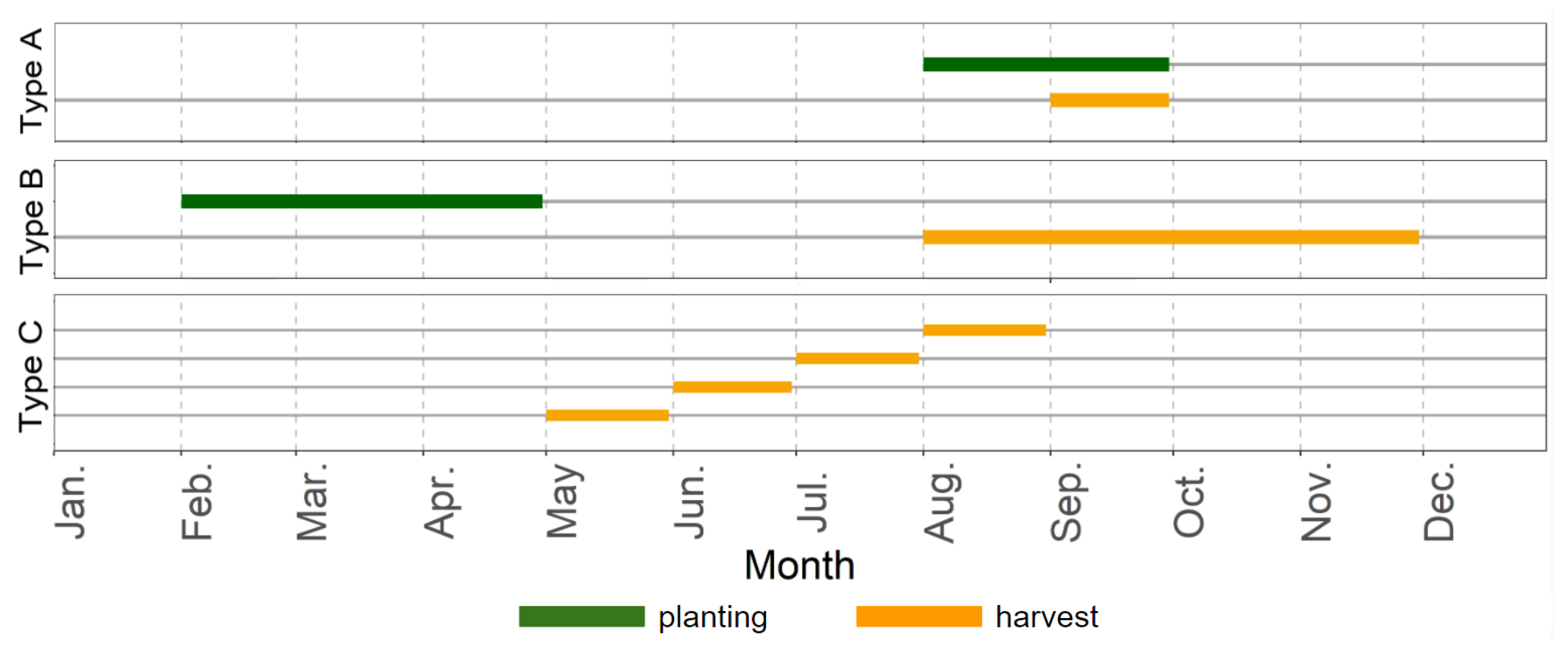
This paper is organized as follows. Section 2 analyzes the climatic conditions and technologies of sugarcane growing in the state of São Paulo, Brazil. Methods for constructing time series of optical (Sentinel-2 NDVI) and SAR (Sentinel-1 coherence) data are described. Section 3 involves the formulation of the algorithm for determining the harvest dates from NDVI time series and the algorithm based on both SAR and optical data. The latter is the development of the algorithm proposed for grain-crops in [24]. Section 4 represents the accuracy analysis of harvest dates and harvested areas determination. In Section 5 some examples of errors in harvest dates determining dates are discussed. The error causes and possible approaches to their elimination are analyzed. In particular, the effect of clouds on the accuracy of harvest date determination according to NDVI is investigated. Finally, the possibility of further development of the proposed algorithms is demonstrated. Section 6 contains the conclusions of the research.

2. Materials

2.1. Study Area

The state of São Paulo is the largest Brazilian sugarcane producer. Since 2006, the satellite images have been used to monitor the sugarcane conditions [8]. The state is located in the south-east of the country and contains 90% of the sugarcane plantings of southern and central Brazil with an area of more than 5.5 mln ha [36]. The state is divided into 645 municipalities and 15 administrative regions, eleven of which grow sugarcane to produce sugar and ethanol. In the rest of the administrative regions (Baixada Santista, Registro, São José dos Campos, and São Paulo) sugarcane is not grown on a commercial scale due to unfavourable climate and terrain features [8].

Vector mask of the sugarcane fields provided by local farmers was used to form a reference sample for 2018. The sample contains 30 fields with an area from 7 up to 419 ha (total area is 3745 ha) located in the municipalities of Araçatuba, Arco-íris, Bentode Abreu, Clementina, Guararapes, Iacri, Inúbia Paulista, Lourdes, Lucélia, Osvaldo Cruz, Parapuã, Piacatu, Rinópolis, Rubiácea, Salmourão, Santo Antônioda Alegria, Santópolis do Aguapeí, and Valparaíso. Figure 1 shows the location of São Paulo, its municipalities, and the study site location as well as some examples of the reference sample fields.

2.2. Sugarcane Harvesting Technologies in Brazil

In Brazil, sugarcane is planted twice a year: in winter (August–September) and summer (February–April) periods. The sugarcane harvest dates are influenced by the local climate. Precipitation affects negatively the sugar content in the sugarcane stalks and creates difficulties with manual harvesting. Therefore, harvest is usually organized during dry periods, when moisture content of the harvested material is low and saccharose concentration is highest. The lowest amount of precipitation is observed in winter. Correspondingly, most sugarcane areas are harvested in one and a half year after the summer planting, and in a year after the winter one (Figure 2) [37]. According to [37], the ratooning harvest begins 10–12 months after the previous harvest.

To monitor the harvest, time series of Sentinel-2 satellite optical data and Sentinel-1 SAR data were used in the research. The optical data advantages are in the shorter time interval (5 days) and high sensitivity of the reflection coefficients in spectral bands to vegetation changes within the fields. The disadvantage is in possible long-term periods of data nonavailability due to the cloud cover. Cloud-independent Sentinal-1 data allow the ability to construct regular time series (except for some gaps due to the changed survey plan). However, for the Brazilian territory, the Sentinel-1 revisiting period is much longer, being 12 days. Taking into consideration the indicated advantages and disadvantages, sets of optical and SAR data were used separately to determine the sugarcane harvest dates.

2.3. Sentinel-2 Optical Time Series

The sugarcane harvest dates were determined based on the search for the characteristic changes in the Sentinel-2 NDVI time series [13]. The Sentinel-2 data are publicly available by the EOS LandViewer service [38]. The research involves 76 scenes of Level-1C Sentinel-2 NDVI in descending mode (granule L1C_T22KEB_A018382, afternoon at 01h32 UTC—morning at 10h32 BRT).

The NDVI time series were constructed using EOS Statistics API [39]. The harvest dates were identified by visual interpretation of the Sentinel-2 MSI images obtained from the EOS LandViewer service [38].

Preliminary studies show that a lot of sugarcane fields are harvested by parts. Dimensions of those parts are often from 5 to 10 ha. Rapid decrease or sharp drop of NDVI down to the value of 0.20–0.30 corresponds to the harvest period. The NDVI drop within a small field fragment is hard to trace from time series of average NDVI. To do that, large fields should be divided into parts, in which the index decrease will be more detectable.

The field polygons were divided by a grid into square parcels (cells) of 10 ha area. Cell fragments with an area less than 1 ha generated by intersecting the grid with the polygon boundaries, were not considered. The number of cells is 574.

The time series was extended by 2 months after the end of the monitoring period. Additional time interval is required to monitor the NDVI change after possible drop at the end of the calendar year to eliminate NDVI false minimums due to clouds and the ones not related to harvest. Thus, the NDVI time series was constructed on the interval of 1 January 2018–28 February 2019.

2.4. Sentinel-1 SAR Time Series

The research involves 30 C-band (5.405 GHz) Sentinel-1 SAR images in descending mode (path 97, frames 659 and 665, slices 1 and 2, morning at 08h53–08h55 UTC—morning at 05h53–05h55 BRT) (Figure 3). All the Level-1 SLC images are acquired in the Interferometric Wide (IW) swath with VV and VH polarization. The choice of the SLC-product is stipulated by the fact that the algorithm of harvest dates determination proposed in the paper relies on the coherence time series, which construction needs the information concerning amplitude and phase of a radar signal. The data in VV polarization, being more sensitive to harvest-related changes in plant height, were used [24]. The coherence time series with a time interval of 12 days and a spatial resolution of 15 × 15 m was constructed.

The images were obtained from the European Space Agency (ESA) Copernicus Open Access Hub [40] and Alaska Satellite Facility (ASF) VERTEX service [41]. The image pairs were processed using the ESA Sentinel Application Platform (SNAP) 7.0 (Sentinel-1 Toolbox) software [24,42]. It included the following steps of pre-processing:

• Applying Orbit Information about satellite position during the SAR data acquisition.
• Back Geocoding—coregistration of two split products based on the orbit information added in the previous step and information from a digital elevation model.
• Coherence Estimation. Coherence is calculated as a separate raster band and shows how similar each pixel is between the slave and master images on a scale from 0 to 1.
• TOPSAR Deburst—removing the seam lines between the single bursts.
• Multilook—speckle reduction.
• Range Doppler Terrain Correction—geocodes the image by correcting SAR geometric distortions using a digital elevation model and producing a map projected product.

3. Methodology

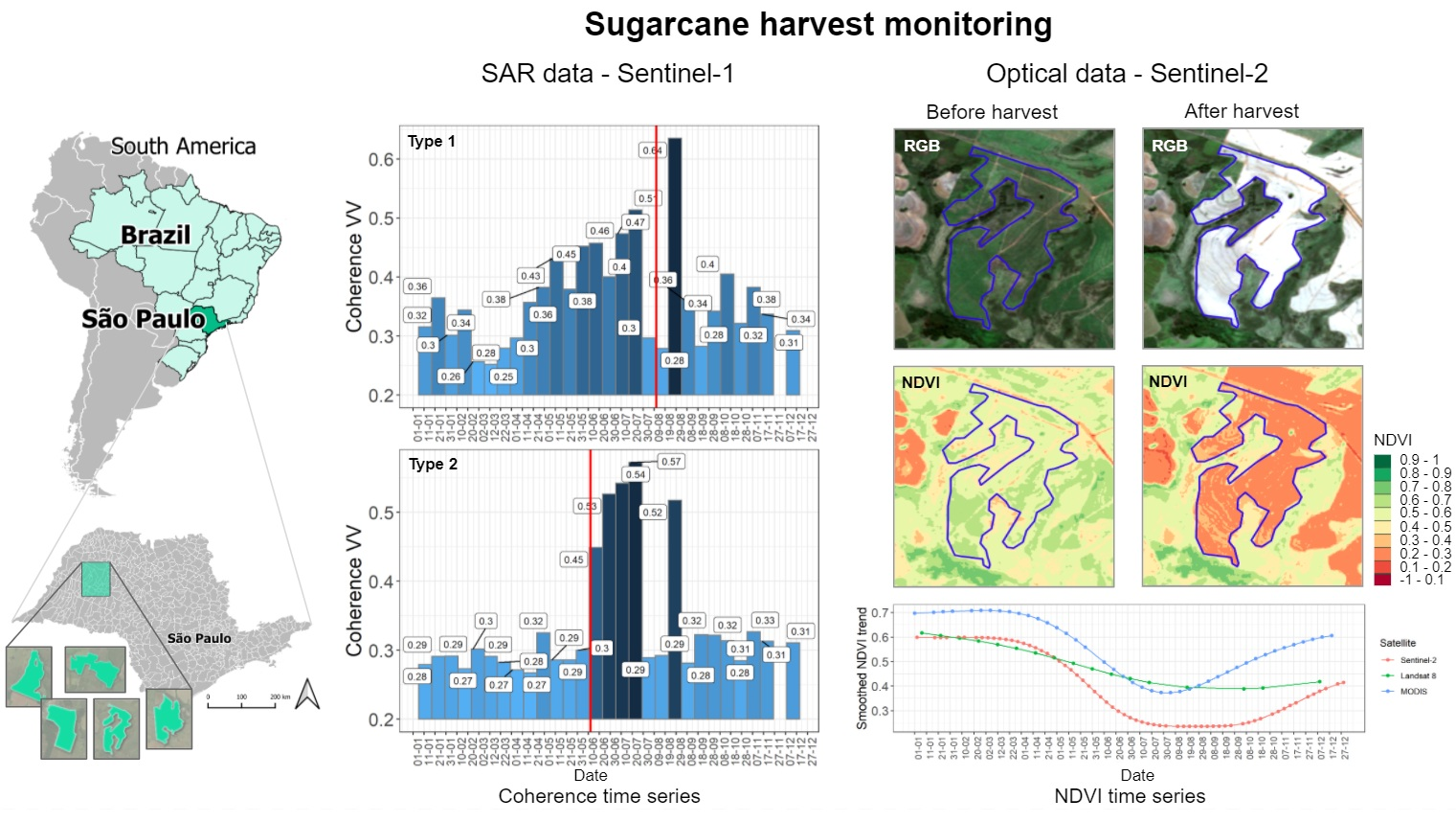
The sugarcane harvest monitoring includes two independent algorithms of harvest date determining based on the decision trees generated from time series of optical and SAR data respectively. Time series of the average Sentinel-2 NDVI values and average Sentinel-1 SAR coherence in VV polarization at the level of a grid cell were calculated for test sugarcane fields. The NDVI data are also used to check and clarify the SAR algorithm results.

3.1. Optical Data

Each parcel has the time series composed of N images. $NDV{I}_i$ is the parcel average NDVI calculated for the ith image $(i=1,2,\dots ,N)$, $T_i$ is the date of the ith image.

The main stage of the sugarcane harvest is stalk cutting in separate stripes according to the terrain features. Depending on the growth process and crop rotation plan, the cut stalks are either left unaffected (ratoon) or harvested completely with the following parcel plowing. In both cases, harvest results in sharp NDVI decrease (Figure 4).

As a rule, short-term periods of NDVI decrease with its following increase up to the previous values are caused by clouds or cloud shadow. The modified median filter is used to smooth them.

A standard median filter [43] smoothes the time series fragments with high NDVI located among the dates with dense clouds (in Figure 5 it should be noted the lack of NDVI local peak in the middle of November as a result of median filtering). That may result in the loss of harvest dates. Hence, the filter was modified to use the median data $\mathrm{med}\left(NDVI\right)$ only where they exceed the NDVI values of the initial time series.

$$NDVI\leftarrow max\{NDVI,\mathrm{med}(NDVI\left)\right\}.$$

(1)

Following conditions should be met for the harvest date $T_{i_k}$:

$$k=\left\{i|NDV{I}_{i-1}-NDV{I}_i\ge \mathsf{\Delta }NDVI\right\}$$

(2)

$$\left\{i_k|NDV{I}_{i_k-1}\ge NDV{I}_{prev}\&NDV{I}_{i_k}\le NDV{I}_{harv}\right\}.$$

(3)

$$\left\{i_k|\exists T_j\in [T_{i_k};T_{i_k}+\mathsf{\Delta }T],NDV{I}_j\ge \mu ·NDV{I}_{i_k-1}\right\}.$$

(4)

Condition (2) means that NDVI decreases sharply in the harvest date $T_{i_k}$—not less than by $\mathsf{\Delta }NDVI$ comparing to the previous date. According to condition (3), the before-harvest NDVI should be rather high. Otherwise, the NDVI decrease may be caused not by the harvest but by the field plowing. The NDVI threshold value during the harvest date $NDV{I}_{harv}$ takes into account different harvesting technologies. The $0.3<NDVI\le 0.4$ values correspond to the parcels with moderate and sparse vegetation [44]. Condition (4) represents the fact that harvest causes long-term NDVI decrease: if NDVI is not raised up to the level of $\mu ·NDV{I}_{i_k-1}$ within $\mathsf{\Delta }T$ period, then harvest was carried out at $T_{i_k}$ moment. The $\mu \in [0;1]$ coefficient compensates insignificant NDVI fluctuations as well as the effect of clouds during the NDVI decrease period.

Thus, the algorithm of determining the harvest dates according to the optical data consists of:

• preliminary filtration (1) of time series $NDV{I}_i$ $(i=1,2,\dots ,N)$;
• control if conditions (2)–(4) are met.

The main algorithm parameters are as follows: $\mathsf{\Delta }NDVI$, $NDV{I}_{prev}$, $NDV{I}_{harv}$, $\mathsf{\Delta }T$, and $\mu$.

To check if condition (4) is met for the harvest dates falling on the end of a calendar year, the NDVI time series should be prolonged by $\mathsf{\Delta }T$ beyond the limits of a harvest monitoring interval.

3.2. SAR + Optical Data

The satellite derived observations for sugarcane show a dynamic pattern similar to wheat and other crops [24,45]:

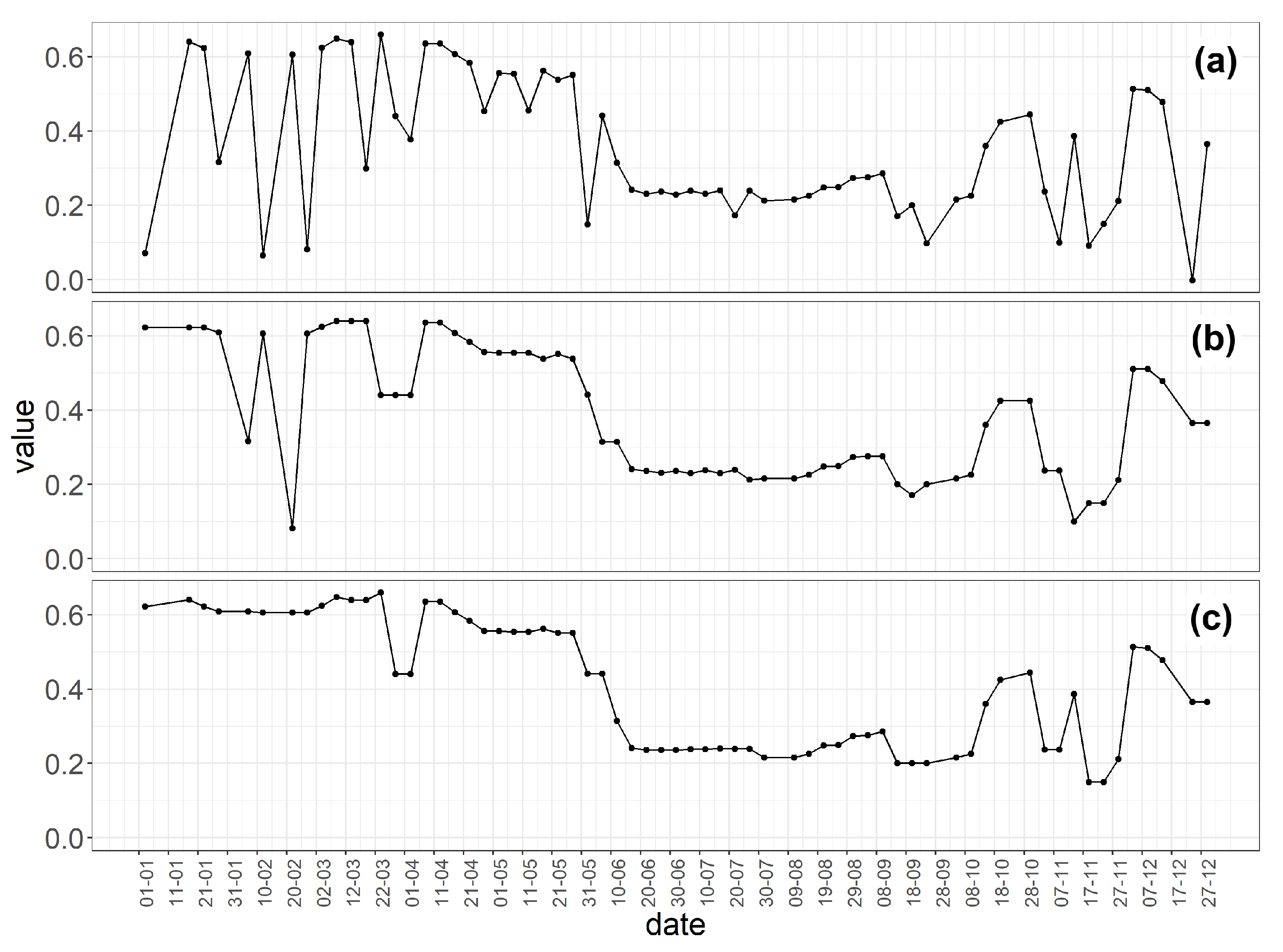
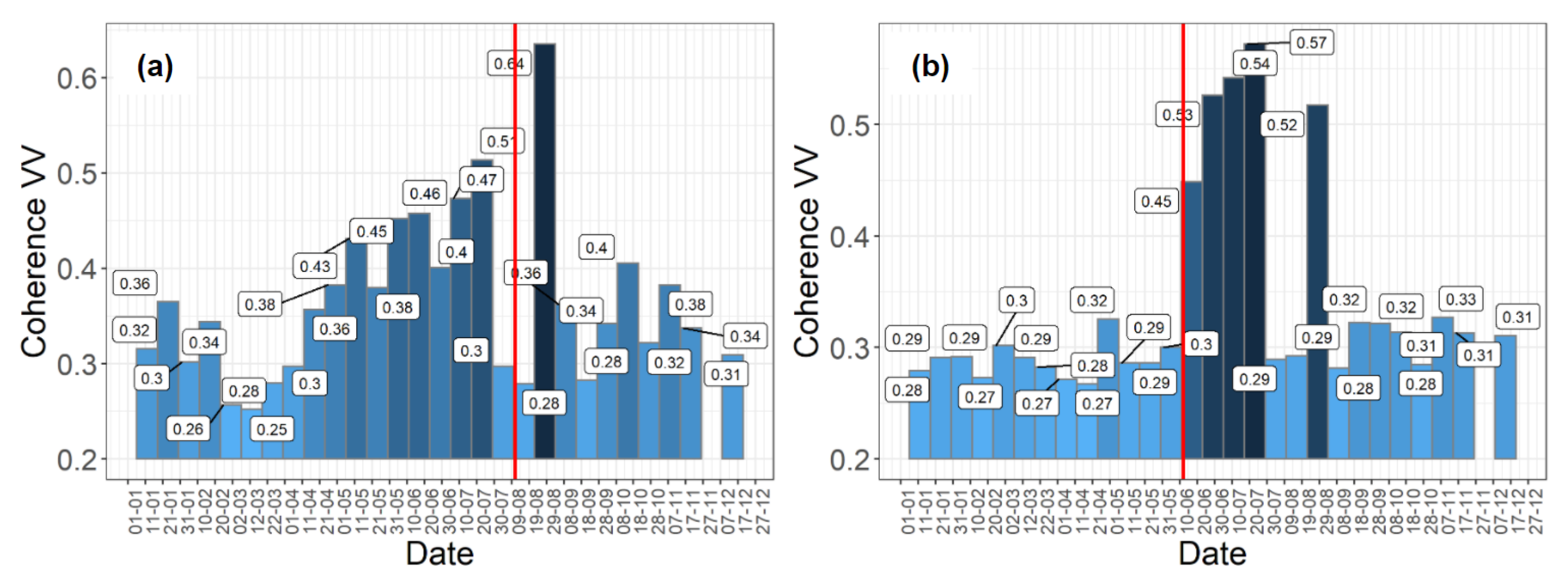
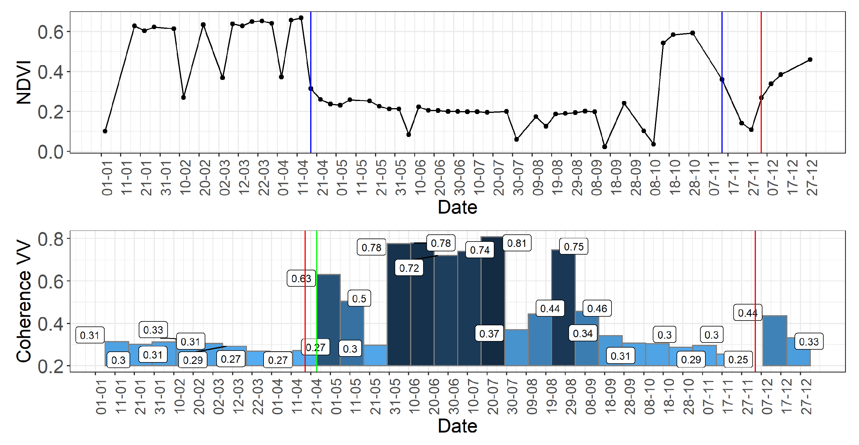
• Slow increase of coherence when the crop gradually dries out (Figure 6a, 12 April–29 July 2018). Then, it drops due to harvest (Figure 6a, 29 July–22 August 2018). Intermittent growth of coherence (Figure 6a, 22 August–3 September 2018) shows that the field is harvested.
• Low and practically unchangeable coherence (Figure 6b, 6 January–11 June 2018), characteristic for dense sappy vegetation cover, drops to low coherence at harvest. High coherence values (Figure 6b, 11 June–29 July 2018) show that the field is harvested.

It should be noted that optical sensors are capable to determine the harvesting operations immediately at the surveying moment while the SAR data help identify the fact of harvest completion, and determine high coherence peculiar for the bare soil, sparse vegetation, and harvest residues. Nevertheless, both cases deal with the algorithm for harvest date determination.

The algorithm for determining the sugarcane harvest date from SAR data is based on the algorithm from Kavats et al. [24]. It searches for the patterns of coherence time series of types 1 and 2, and assessing the vegetation cover density after possible harvest from the backscattering coefficient ${\sigma }^0$. In contrast to [24], the study uses NDVI to estimate the vegetation state. Use of Statistics API to generate NDVI time series helped save the disk space and time required before to store and process ${\sigma }^0$ data. Moreover, other improvements are introduced in the algorithm [24] representing the features of sugarcane cultivation and harvest.

Consider the proposed algorithm in more detail. Take $M+1$ time-ordered SAR SLC images. Denote the date of the ith image by $T_i$ $(i=1,2,\dots ,M+1)$. Calculate the coherences between ith and $(i+1)$th images as it is shown in Section 2.4. Generate a time series of the field-average coherence values $C_i$ $(i=1,2,\dots ,M)$.

To search for the time series patterns corresponding to the harvest, calculate the differences of coherences $\mathsf{\Delta }{C}_i=C_{i+1}-C_i$ $(i=1,\dots ,M-1)$ and determine the directions of their changes $D{C}_i$

$$D{C}_i=\left\{\begin{array}{cc}0,\hfill & |\mathsf{\Delta }{C}_i|\le \epsilon ,\hfill \\ 1,\hfill & \mathsf{\Delta }{C}_i>\epsilon ,\hfill \\ -1,\hfill & \mathsf{\Delta }{C}_i<-\epsilon .\hfill \end{array}\right.$$

The $\epsilon$ threshold is chosen so that the coherence change $\mathsf{\Delta }{C}_i$ within the range of $[-\epsilon ;\epsilon ]$ could be considered as insignificant.

Harvest either results in coherence drop ($D{C}_i=-1$) or does not change it comparing to the previous period ($D{C}_i=0$). After harvest, coherence grows ($D{C}_i=1$). Thus, harvest corresponds to the transfers $D{C}_i\to D{C}_{i+1}$ of type: $0\to 1$ or $-1\to 1$. Introducing the second differences $D^2{C}_i=D{C}_{i+1}-D{C}_i$ write down the conditions of coherence change corresponding to the harvest

$$\begin{array}{c}\hfill D^2{C}_i=2,\end{array}$$

(5)

$$\begin{array}{c}\hfill D^2{C}_i=1\&D{C}_{i+1}=1.\end{array}$$

(6)

Condition (5) corresponds to the time series of type 1 coherence; and condition (6) corresponds to the time series of type 2 coherence. Conditional check $D{C}_{i+1}=1$ is meant for eliminating from the analysis the transfers $D{C}_i\to D{C}_{i+1}$ from $-1$ to 0. The latter may be caused by the beginning of harvest but not by its completion.

When the harvest is over, one can usually observe considerable growth of coherence. Thus, introduce the additional condition, when (5) and (6) are checked

$$\mathsf{\Delta }{C}_{i+1}>\theta ,$$

(7)

where $\theta >\epsilon$.

Table 1. Connection between the time series indices.

i	T	C	$\mathsf{\Delta }\mathbf{C}$	$\mathbf{DC}$	${\mathbf{D}}^2\mathbf{C}$
1	$T_1$	$C_1$
2	$T_2$	$C_2$	$\mathsf{\Delta }{C}_1$	$D{C}_1$
3	$T_3$	$C_3$	$\mathsf{\Delta }{C}_2$	$D{C}_2$	$D^2{C}_1$
…	…	…	…	…	…
M	$T_M$	$C_M$	$\mathsf{\Delta }{C}_{M-1}$	$D{C}_{M-1}$	$D^2{C}_{M-2}$
M + 1	$T_{M1}$

demonstrates connection between the time series indices. Thus, index i, determined from the conditions (5)–(7), corresponds to the harvest date $T_{i+2}$.

Check the identified potential harvest dates using the NDVI time series. The checking is based on the following assumptions:

• harvest is carried out in terms of NDVI descending trend;
• on the harvest completion, NDVI should be low.

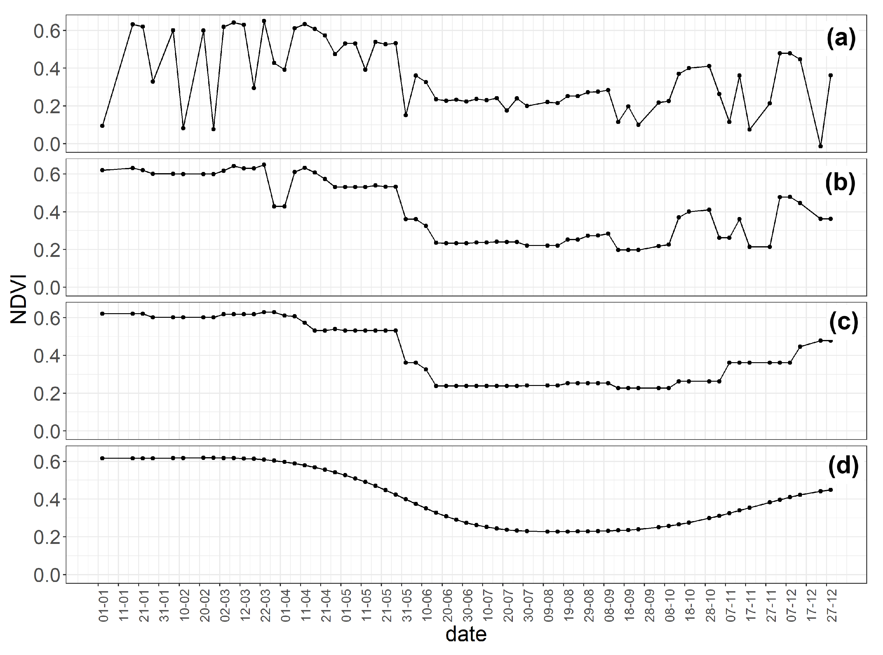
The NDVI trend construction consists of three stages (Figure 7):

• Filtration of short-term NDVI drops caused by clouds and cloud shadows using the modified median filter (1);
• Averaging of the NDVI series using the median filter with wide window;
• Spline-smoothing.

Harvest condition on the descending NDVI trend:

$$trend{\left(NDVI\right)}_l-trend{\left(NDVI\right)}_{l-1}<0$$

(8)

where $l-1$ and l are the numbers of optical images before and after the potential harvest date.

After the harvest, NDVI should be low.

$$trend{\left(NDVI\right)}_l\le NDV{I}_{hd}.$$

(9)

That condition is similar to the second condition from (3) for the algorithm based on the optical data.

Gradual coherence growth before harvest (Figure 6a) may be caused not only by the plant drying-out but by the partial field harvest. The harvested part is empty, and it has high coherence, while the rest of the field is of low coherence. Along with the increasing harvest area, average field coherence grows gradually so that one cannot observe the fast coherence growth upon the harvest completion. As a result, the harvest date is not determined from the conditions (5)–(7). Irrespective of that, high coherence is observed within the parcel upon the harvest completion.

Single out the members of time series $C_h$ $(h\in 1,\dots ,M)$ with high coherence

$$C_h>C_{hi}.$$

(10)

High coherence values correspond to the sparse vegetation or bare soil. Consequently, harvest may be carried out only after a long period from the last date with high coherence $T_h$. Denote the potential harvest date by $T_I$ and introduce the checking

$$T_I\le T_h\mathrm{OR}{T}_I>T_h+\mathsf{\Delta }{T}_{hi}.$$

(11)

where $\mathsf{\Delta }{T}_{hi}$ is the minimum time period required for the plant growth.

Finally, if the harvest dates are not determined from the patterns of coherence time series (5)–(7) and conditions (8)–(11), check the dates of high coherence (10) as for their meeting the conditions (8), (9), and (11).

Thus, the algorithm of harvest monitoring in terms of the SAR and optical data consists of the following steps:

• Searching for the rapid changes in coherence corresponding to types 1 and 2 (5)–(7).
• Checking the dates determined from NDVI (8), (9).
• Checking the potential harvest dates, left after step 2, as for their following the high coherence dates (11).
• If no harvest dates are found in steps 1–3, perform steps 2–3 for high coherence dates (10).

The algorithm parameters are: $\epsilon$, $\theta$, $NDV{I}_{hd}$, $C_{hi}$, $\mathsf{\Delta }{T}_{hi}$.

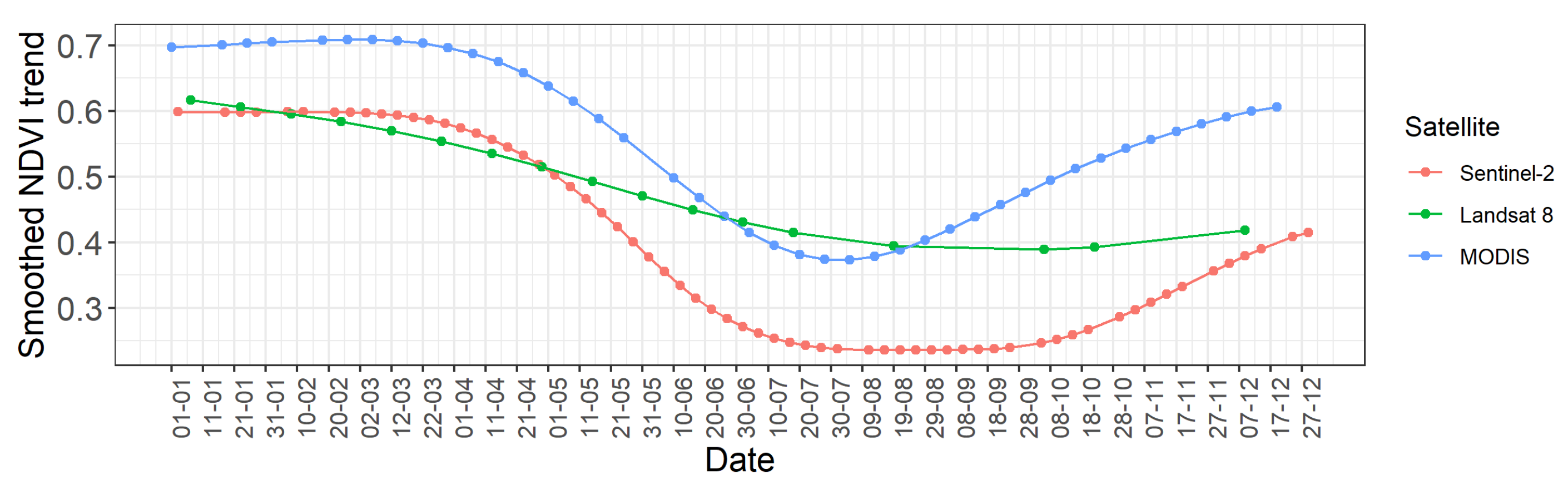
It should be noted that the use of NDVI trend does not mean the determining of harvest dates from optical data. Comparing to the data used in the optical algorithm, the NDVI trend may derive from the data of much lower spatial resolution and/or periodicity: MODIS, Landsat, etc. (Figure 8).

3.3. Quality Metrics

Metrics are needed to evaluate (1) the quality of harvest dates determining, (2) the sugarcane area harvested in a month.

Each complete or partial field harvest must be determined. Since the reference harvest dates are determined by visual interpretation of the optical data being the same with the data applied in the algorithm, it is incorrect to assess the error of harvest dates determining with the help of traditional error metrics, such as mean absolute error or root mean square error. To assess the quality of harvest dates determining, the

Table 2. Table of the quality assessment for harvest dates determining.

	Match	Not-Match
Match	True Match	False Match
Not-match	False Not-match

is used. The table columns correspond to the harvest dates for the reference data; the rows correspond to the harvest dates determined with the help of the algorithm.

True Match is the number of coincidences of harvest dates. The algorithm error is the total of false responses (False Match) and omissions (False Not-match) of the harvest dates. Introduce also the following

$$\mathrm{True}\mathrm{match}\mathrm{rate}=\frac{\mathrm{True}\mathrm{Match}}{\mathrm{True}\mathrm{Match}+\mathrm{False}\text{Not-match}}$$

and

$$\mathrm{Match}\mathrm{predictive}\mathrm{value}=\frac{\mathrm{True}\mathrm{Match}}{\mathrm{True}\mathrm{Match}+\mathrm{False}\mathrm{Match}}.$$

True match rate shows the proportion of matches for harvest dates determined by the algorithm from the total number of harvest dates of the reference sample. Match predictive value shows the proportion of matching harvest dates among all dates found by the algorithm.

Estimation of the sugarcane area harvested per month is rather useful for practical applications. The harvested area is determined by harvest end dates for cells. The harvest end date is the last date in the sequence of harvest dates for a cell, separated by a time interval less than one month.

4. Results

4.1. Determining of the Harvest Dates by the Optical Data

The calculations were carried out in terms of the following parameters: $\mathsf{\Delta }NDVI=0.08$, $NDV{I}_{prev}=0.3$, $NDV{I}_{harv}=0.4$, $\mathsf{\Delta }T=40\mathrm{days}$, and $\mu =0.9$. Window width of the modified median filter is $k=3$.

The results of quality assessment for the harvest dates determining are: True Match = 45, False Match = 39, False Not-match = 32, True match rate = 0.58, Match predictive value = 0.53.

Figure 9 represents the general distribution of harvest dates determined from the optical data.

Dynamics of the average fraction of the cloud-covered image area (Figure 10a) is determined from Sentinel-2 images metadata (cloudy pixel percentage). According to the graph, the most favourable observation conditions were during the period of March–August 2018 when the cloud fraction was not more than 45% of the image area. It is no wonder that the overwhelming majority of the harvest dates coincidences fall on the period from March to August 2018 (Figure 10b).

Omissions of the harvest dates have two clear maximums. The June maximum falls on the low-cloudiness period. According to Figure 9, there are comparatively minor errors of the harvest dates determining during that period; they are rarely more than 10 days. The October minimum falls on the end of the year—a period of dense clouds.

There is a similar situation for false responses (Figure 10b). The June maximum corresponds to the comparatively minor errors in the harvest dates determining since both false responses and omissions fall on June. Such errors will not affect the evaluation of the sugarcane area harvested within that period. Apparently, the September maximum of false responses is related to the October omissions of harvest dates (Figure 10b): first, there is a false response of the algorithm due to the cloudiness; it is followed by the omission of the real harvest date. The November maximum of false responses is also connected with cloudiness since the cloud-cover peak falls on November 2018.

4.2. Calculation of the Harvested Areas

The harvested area was calculated according to the dates of cells harvest completion. To do that, the determined harvest dates for each cell were divided into the sequences with a time lapse between the neighbouring dates not more than 30 days. The last dates of those sequences were considered the dates of cells harvest completion.

The harvested areas are calculated for both analyzed algorithms. The optical algorithm parameters are as follows: $\mathsf{\Delta }NDVI=0.08$, $NDV{I}_{prev}=0.3$, $NDV{I}_{harv}=0.4$, $\mathsf{\Delta }T=40\mathrm{days}$, $\mu =0.9$, and $k=3$. The SAR-optical algorithm parameters are as follows: $\epsilon =0.05$, $\theta =0.07$, $NDV{I}_{hd}=0.4$, $C_{hi}=0.5$, and $\mathsf{\Delta }{T}_{hi}=40\mathrm{days}$.

Figure 11 and

Table 3. The areas harvested within a year.

Method of Calculation	Area, ha
Visual interpretation	3522.22
Optical algorithm	3421.40
SAR + Optical algorithm	3157.59

represent the calculation results.

According to Table 3, it could be seen that the harvested areas evaluated by the results of the optical algorithm coincide with the harvested areas evaluated by a visual interpretation by 97%. For SAR + optical algorithm such coincidence is 90%.

According to the Figure 11, it is quite clear that the combined algorithm determines the harvested areas worse than the algorithm based only on the optical data. That is due to a much longer interval between SAR images (12 days compared to 5 days for Sentinel-2); thus, the harvested area is recorded with time delays. The delays in identification of the harvest dates may be also explained by other field operations changing the distribution of reflectors and reducing the coherence. To estimate the effect of that factor, one needs more accurate data on the operations within the field. Finally, the greatest determination errors are possible due to the lack of one of the SAR images in November 2018.

5. Discussion

The causes of the errors in determining the harvest dates are considered below and a way of possible improvement to the algorithms is specified.

5.1. Analysis of the Time Series

Consider the causes of the errors on the examples of time series for several cells.

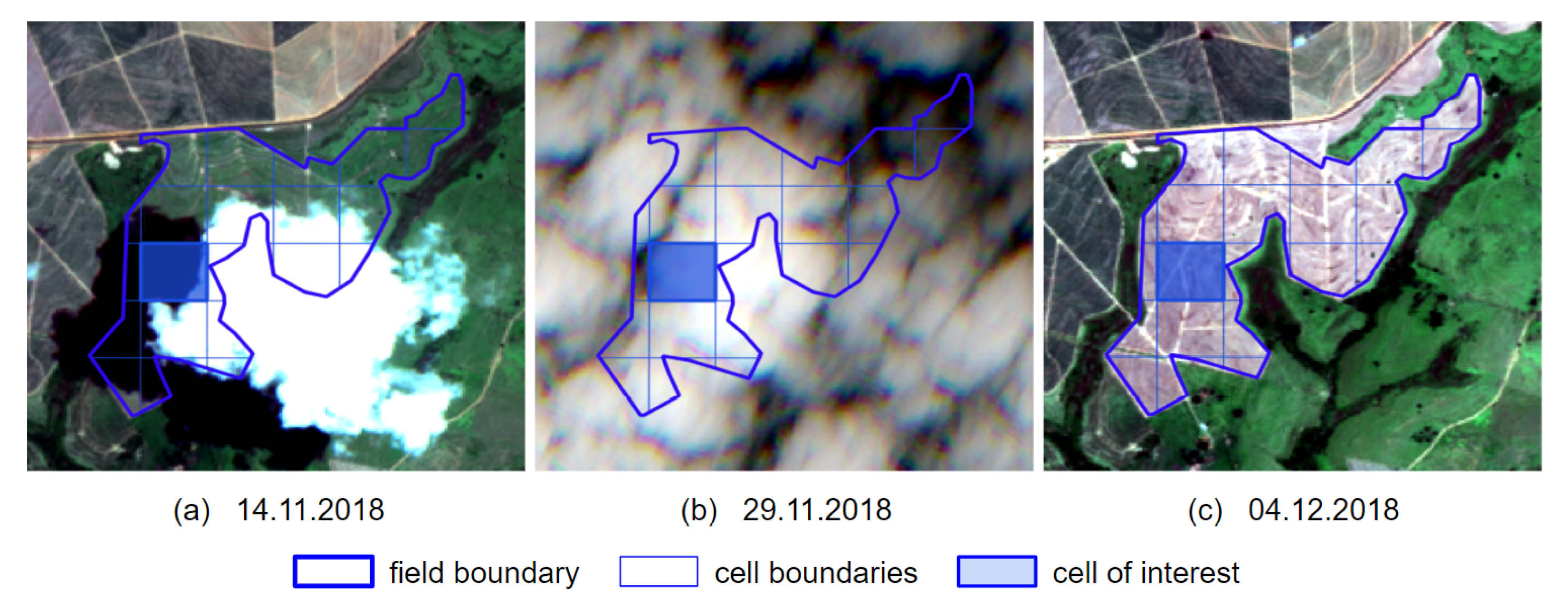
Lengthy cloudiness impedes the construction of a regular NDVI time series during the harvest period. For the cell shown in Figure 12 and Figure 13 (cid is cell id), the April harvest date (18 April 2018) is determined correctly by both algorithms. The December harvest date (4 April 2018) is preceded by dense clouds (Figure 13a,b), resulting in a false response of the optical algorithm in November. The real harvest date is omitted due to the lack of the NDVI decrease required by the algorithm. According to the SAR data, harvest was in early November–early December. Harvest date cannot be determined more accurately as there is no SAR image in December. However, the behaviour of time series of the SAR data holds out the hope that the date can be identified in case of the available image.

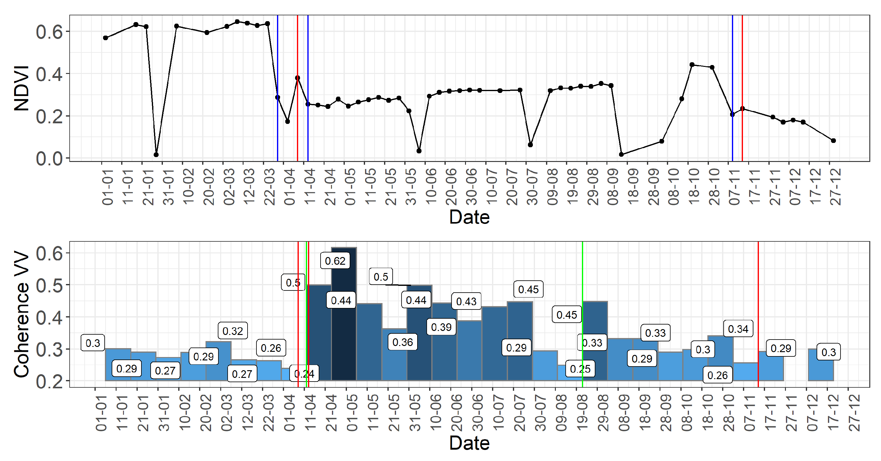
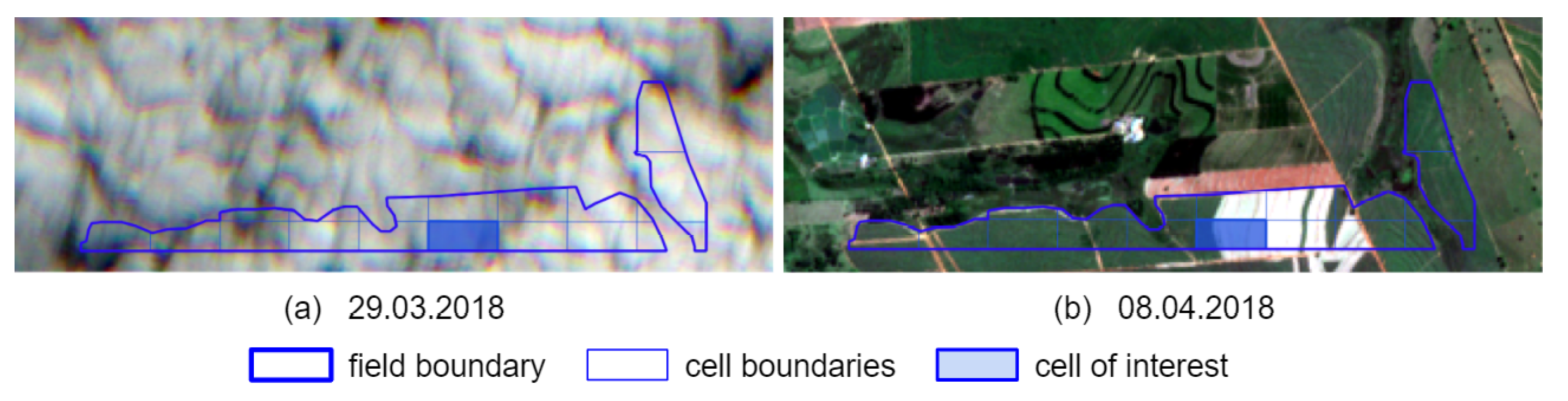
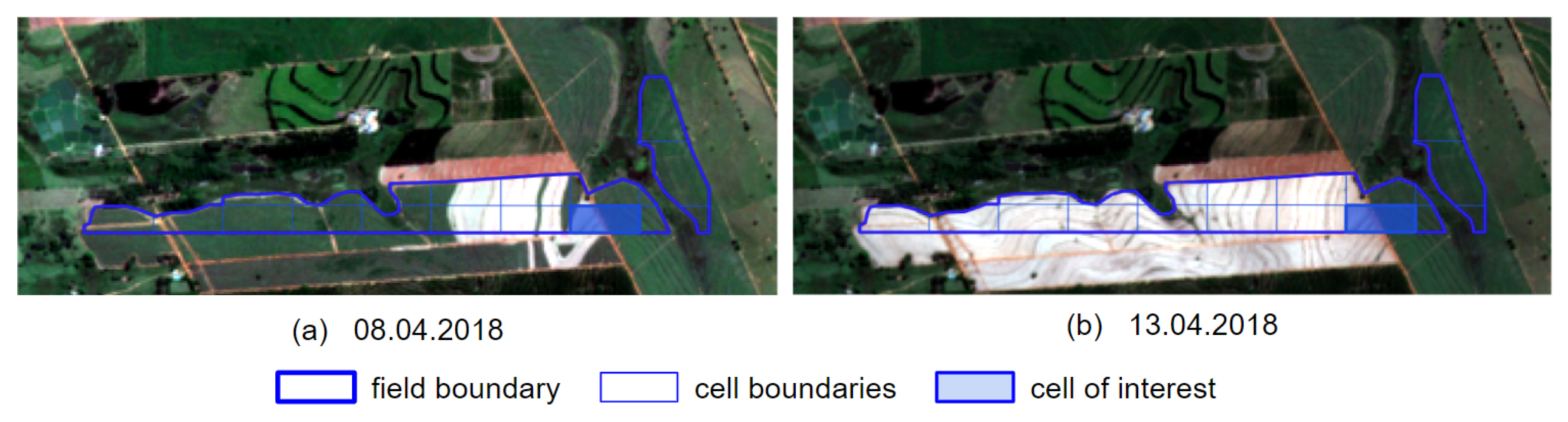
Cloudiness results in the NDVI drop within late March (29 March 2018) while harvest takes place actually in early April (Figure 14 and Figure 15). The date of the harvest completion in April (13 April 2018), determined according to the optical data, may be corrected according to the SAR data as the date of 12 April 2018 shows high coherence. Apparently, false response of the SAR algorithm in August is connected with some agrotechnical operations within the field. The November harvest date is omitted by the SAR algorithm due to the image lack. The optical algorithm responds early due to dense clouds.

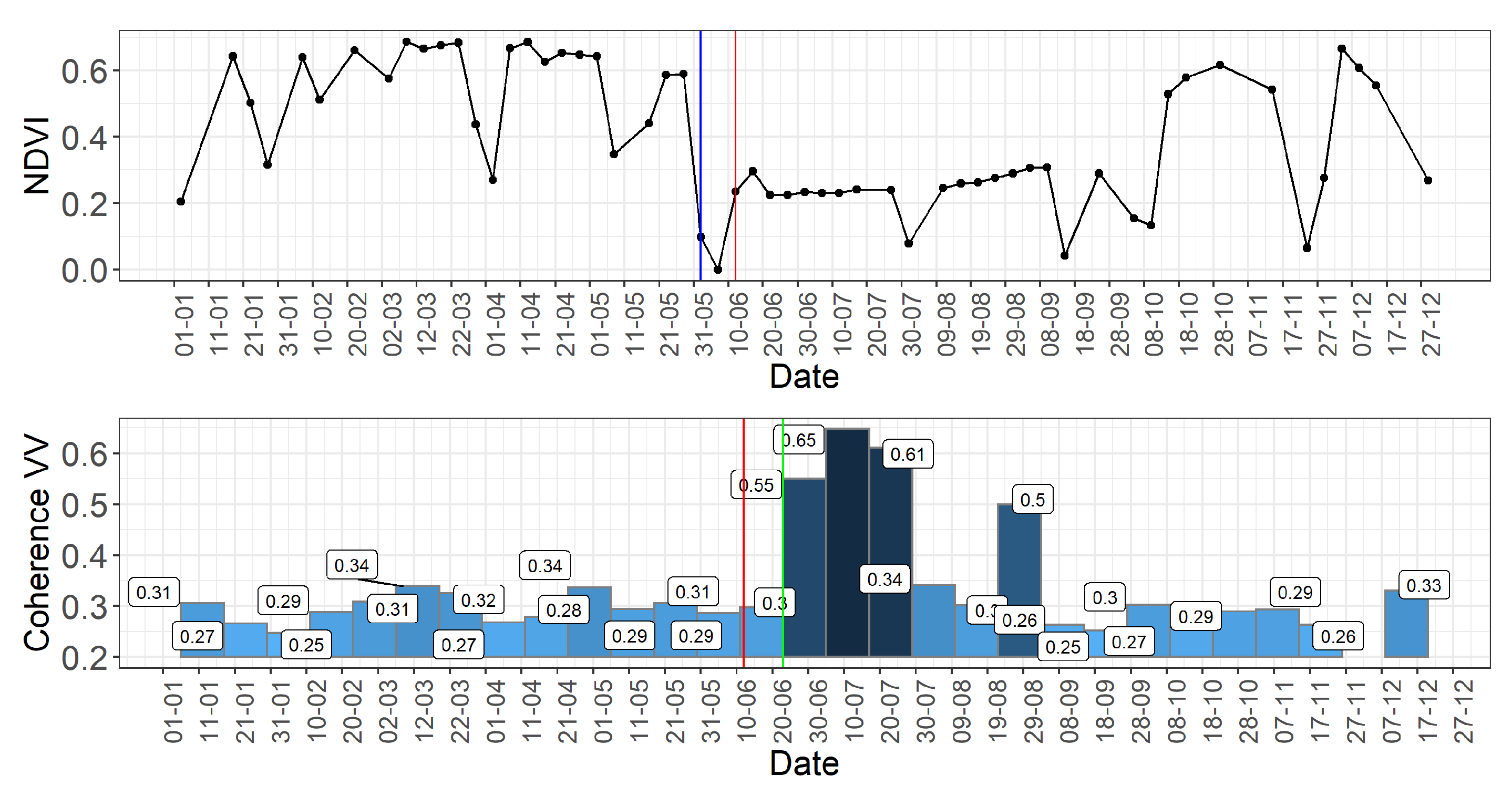
As before, the early response of the optical algorithm is caused by clouds (Figure 16 and Figure 17). SAR algorithm determines the harvest date correctly with all its possible accuracy: an interval between its determined harvest date 23 June 2018 and real harvest date 12 June 2018 does not exceed the interval between surveys. During late June–early August, certain agrotechnical works are carried out within the field resulting in the coherence decrease.

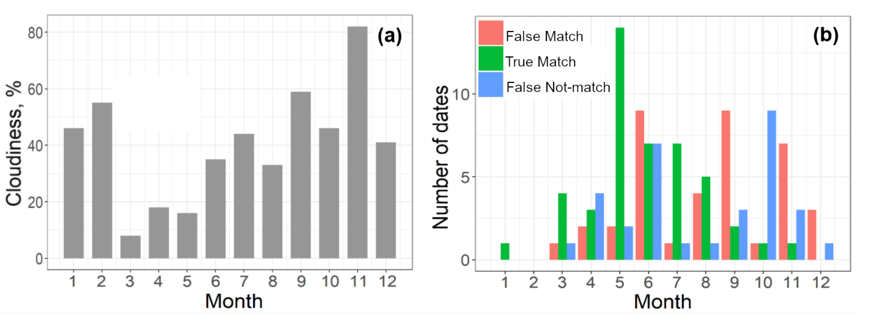
In the case of minor cloudiness, the time delay of the harvest dates determined from the optical data is not more than 5 days relative to the actual dates, which is the characteristic interval between the Sentinal-2 survey within that area. A long-term cloudiness period may result in two errors: preliminary false response and omission of the real harvest date. Clouds cause rapid NDVI drop; during the following harvest, NDVI experiences no decrease as it already has low values. Note that less than 40% cloud cover (Figure 10a) provides a rather accurate evaluation of the harvested areas.

In this case, the harvest dates cannot be determined according to the SAR data during the maximum cloudiness period due to the lack of SAR image in November. Nevertheless, the SAR data allow the ability to clarify the harvest dates obtained by the optical algorithm. Thus, it is most probably that the harvest, falling on the early dates of a high-coherence period, recorded by the optical algorithm took place several days earlier—within the period between optical images (Figure 14, Coherence VV). That allows postponing the harvest date by several days but not more than by five days.

One of the reasons for erroneous algorithm functioning is non-harvest field operations (plantation burning, plowing, etc.); those operations are detected as harvest.

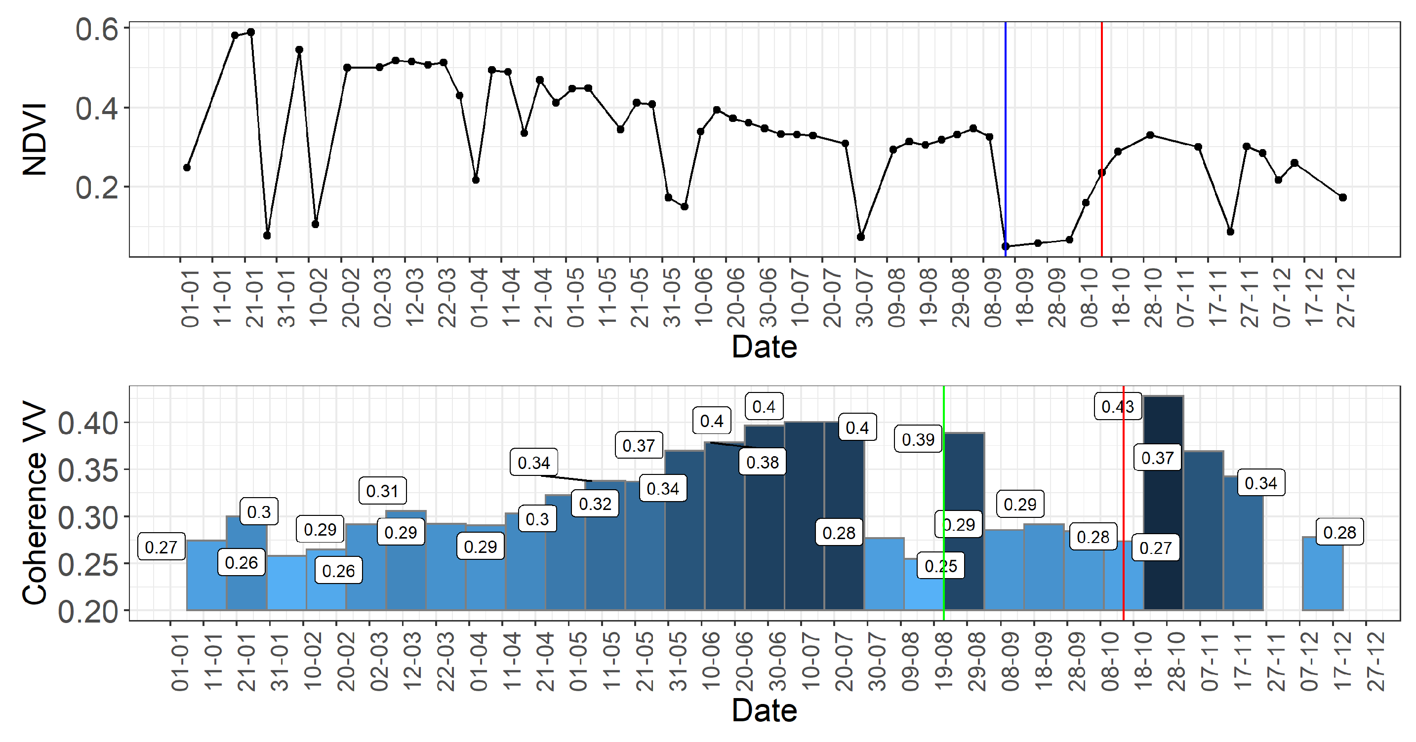
Early September is characterized by the period of dense clouds resulting in a false response of the optical algorithm (Figure 18). The algorithm, relying on the SAR data, determines correctly the harvest in October but determines it falsely in August. Apparently, the coherence decrease in August is caused by the field works. Pay attention to the slow coherence growth during March–July that corresponds to the slow NDVI decrease.

The following group of problems is connected with the erros in field boundaries and inclusion of the nonagricultural lands into its area. Such inclusions change the behavioural pattern of the NDVI and coherence time series, making it impossible to record the fact of harvest.

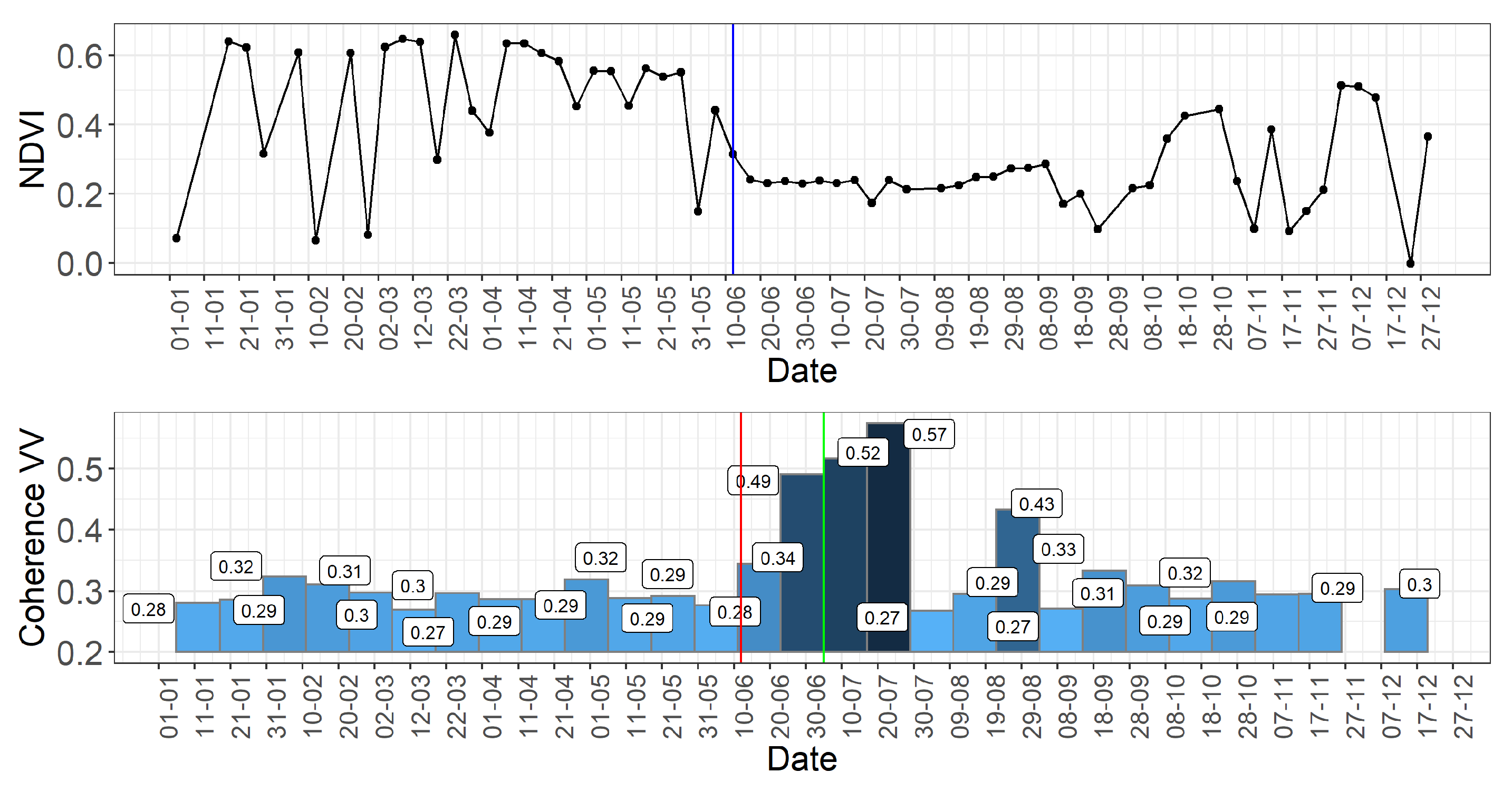
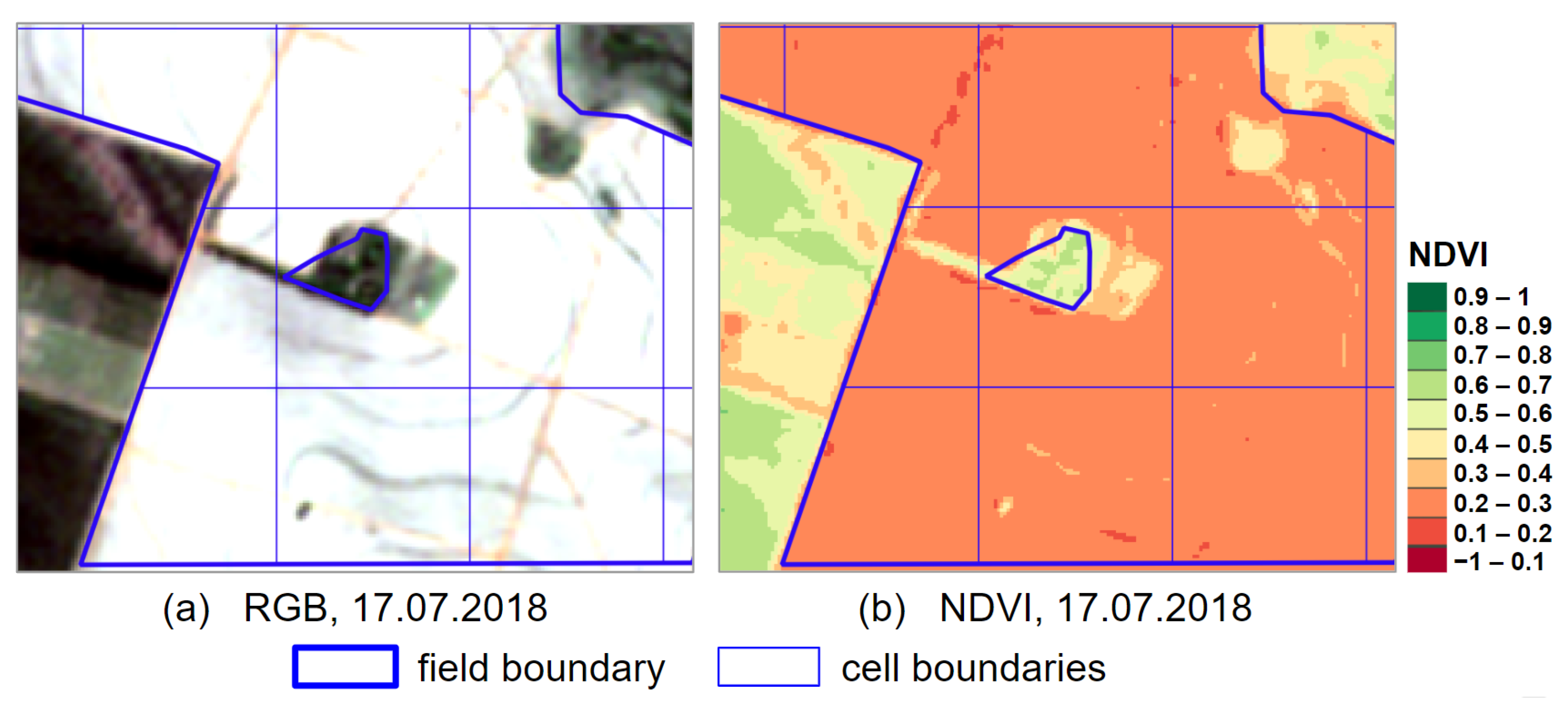
For the spatially heterogeneous cell shown in Figure 19 and Figure 20, the harvest date is determined according to the optical data for 12 June 2018. According to the SAR data, the harvest took place within the period up to 11 June 2018 when the coherence growth begins. However, that date is omitted by the SAR algorithm due to insufficient coherence increase. The latter is caused by the fact that the parcel includes the nonagricultural lands (Figure 20).

Nevertheless, the observed coherence jump violates the behavioral pattern of the time series and results in the harvest date omission. The false response of the algorithm occurs in July. It appears that further coherence drop in late July–early August is connected with the post-harvest operations.

For the cell represented in Figure 21 and Figure 22, a part of the sugarcane parcel is covered with nonagricultural vegetation and has low coherence within the whole season. The first March harvest date was omitted since it did not cause the coherence jump. High coherence appears when most of the parcel is harvested. That happens in June–July. The response of the optical algorithm in September is not confirmed by low coherence values within that period.

Spatial heterogeneity can be the result of a digitization error or inaccuracy in combining several cadastral parcels into a single agricultural field. Incorrect delineation of the field boundaries (Figure 23) has resulted in the fact that the field includes a road and a part of a neighbouring field with other harvest dates.

A sugarcane field is homogeneous if the plants are planted roughly at the same time. As a rule, harvest of such a field takes not more than a month; the next harvest will be only after a long period. All the NDVI jumps or SAR algorithm responses during that period are possible due to the interferences in observations or due to the agrotechnical non-harvest operations within the field. The field homogeneity is good support while identifying the harvest dates.

Plants in a nonhomogeneous field, planted during different periods, are at different development stages; it means that they differ considerably in terms of NDVI value and backscattering of the SAR signal. On such a field, NDVI drop and jump in the coherence growth may be poorly expressed as the harvest covers only some part of the parcel.

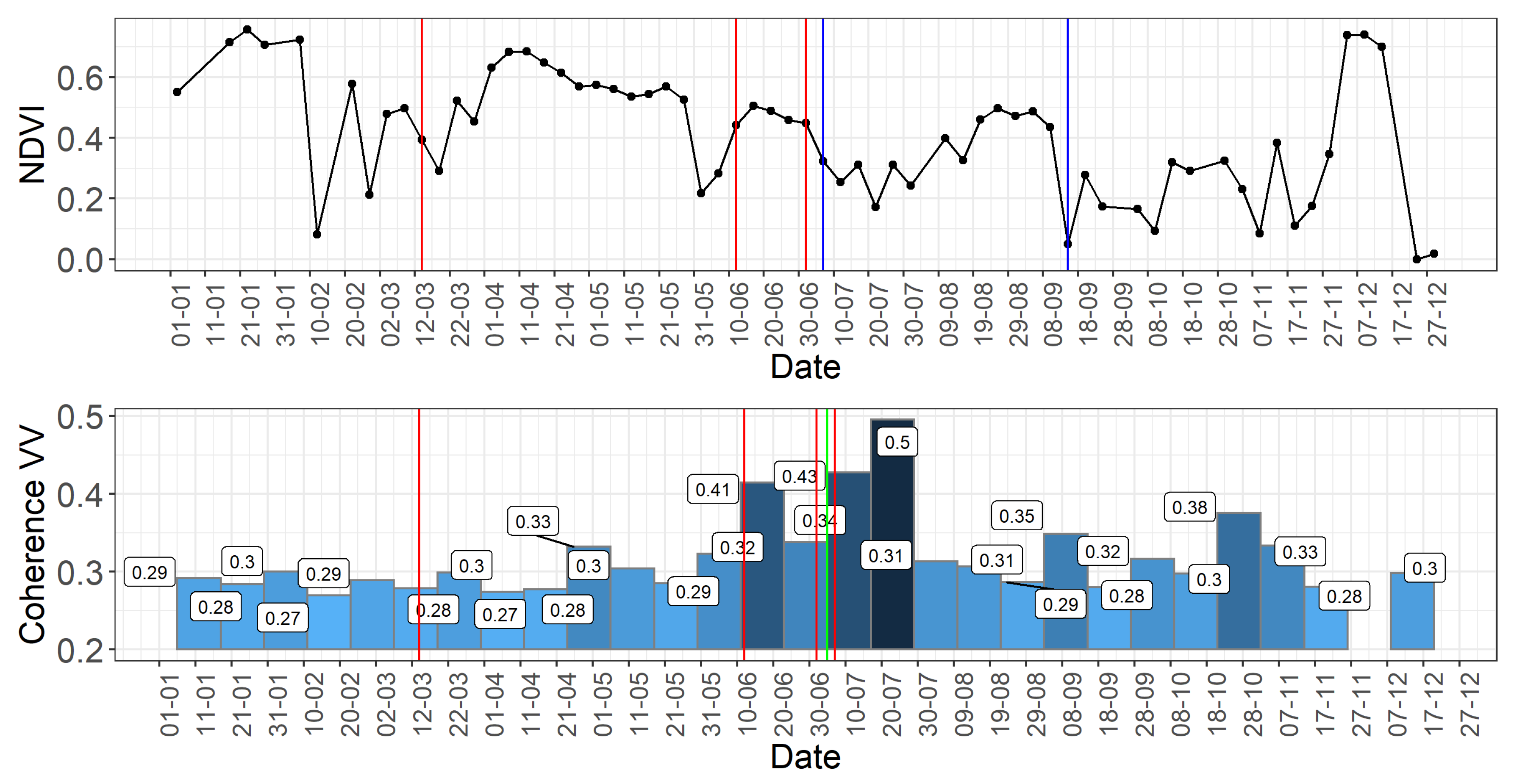
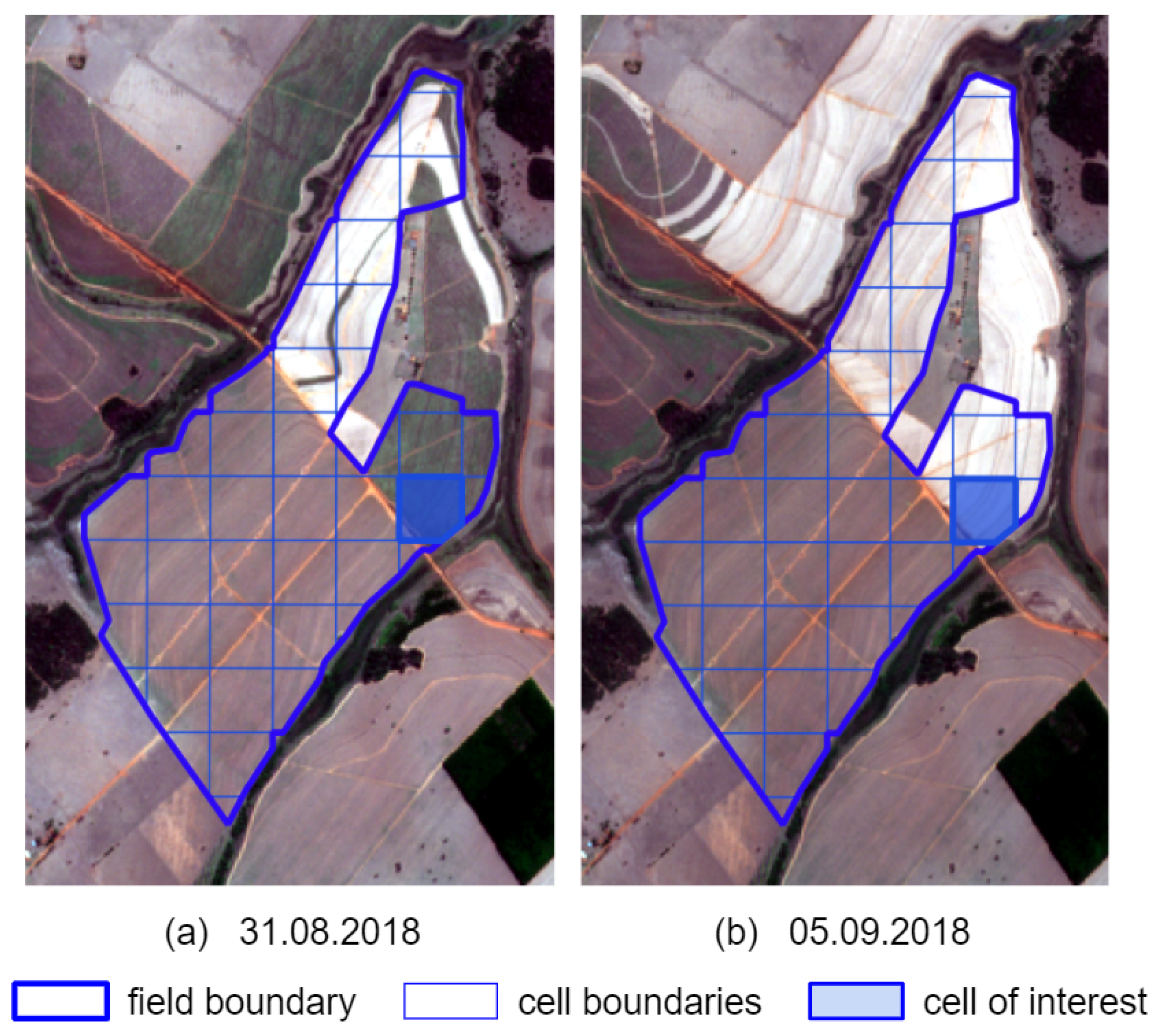
Differences in sowing dates result in harvest different dates for field parts. The optical algorithm demonstrates the premature false response caused by cloudiness for the cell shown in Figure 24 and Figure 25. The SAR algorithm omits harvest in April: due to the harvest of a part of the parcel, coherence growth does not reach its threshold. Instead, there are false responses in June and August. The October harvest date is identified correctly by the SAR algorithm.

Thus, the proposed algorithms will function correctly for the homogeneous fields not including certain parts of nonagricultural lands. It is desirable to divide the nonhomogeneous lands into homogeneous parts. The latter is of special importance for the proper functioning of the algorithm based on coherences data.

5.2. Possible Development of the Algorithms

The division into small parcels has made it possible to reduce nonhomogeneity of the fields and record better the harvest-related NDVI drop. That division was performed from geometrical considerations without taking into account vegetation state. Preliminary field segmentation according to the optical images would allow singling out the homogeneous parcels. In particular, according to Murugan and Singh [46], the use of k-means clustering to single out homogeneous fields, within which the harvest was monitored based on Sentinel-1 ${\sigma }_{VH}^0$, ${\sigma }_{VV}^0$, and AVHRR NDVI time series, provided the overall 82.17% accuracy of the result. It should be emphasized that in this case, the segmentation would result in the increased volume of the processed data.

While supposing a certain duration of the vegetation period of sugarcane, the simplest model of its growth was used implicitly. The use of more advanced mathematical models will be the natural development of that approach. Such a model could forecast a trend, being required for operational monitoring. Gaussian function may be applied to model the NDVI change in time [47].

There were no data concerning the dates of planting or preceding harvest for the parcels under analysis. If there is information about the dates of growth beginning, local climatic and meteorological parameters, and state of soils, it is possible to apply biophysical modeling of the plant growth and development as well as the harvest at different vegetation stages. For instance, Marin and Jones [48] construct a dynamic simulation model of sugarcane growth in Brazil basing on the analysis of biophysical processes in terms of 27 variables for Photosynthesis, Phenology, Leaf Development, Biomass Partitioning, Sucrose Partitioning, Plant Extension, and Root and Water Stress. Extreme learning machine was applied by Ghazvinei et al. [49] to predict the sugarcane growth based on such ground measurements as amount of daily water irrigation, soil electrical conductivity, daily maximum temperature, evaporation, sunshine hours, rainfall precipitation, humidity percentage, and mean wind speed at 2 m above the ground. Such observations would help narrow down the time intervals of harvest dates identification and clarify the results of satellite monitoring, having excluded the deliberately false dates.

Time delay of the harvest dates detected by the SAR algorithms are mostly related to the post-harvest operations. A calendar of agrotechnical operations changing soil surface or vegetation cover state, as well as data on plant growth stage makes it possible to single out the harvest among the operations changing the nature of the radar signal reflection.

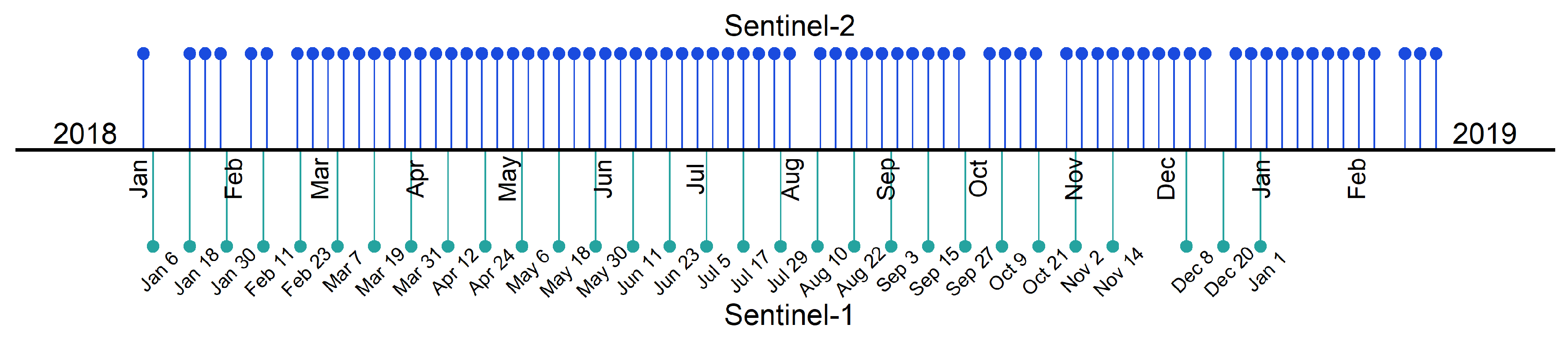
A much shorter revisit time for the study area is the important advantage of the optical data compared to the SAR one. An interval between surveying is 5 days in the case of Sentinel-2 in comparison with 12 days for Sentinel-1. Increasing revisit frequency may improve considerably the algorithm based on SAR data.

The use of textural features in harvest monitoring is one more tendency in the algorithm development. It will require machine learning methods capable of efficient identification and use of such features. Significant advantages can be achieved using high-resolution data (about 1 m), allowing to track changes in field texture associated with the agricultural machinery operation.

Classification methods and artificial neural networks used to detect harvested fields during the harvest monitoring within certain scenes are the alternative for the threshold methods and solution tree. Such algorithms require a large reference sample, which completeness and representativeness affect the accuracy of the results. However, once adjusted decision rule of a classifier will help reduce the following computational costs owing to the processing of individual scenes and no need to construct a long time series. For sugarcane fields in the state of São Paulo, a method of object-oriented classification is applied by Goltz et al. [50] to discriminate different sugarcane harvest types (burnt, non-burnt, or no harvest) for different soil types using Landsat-TM data. There are the following image characteristics (classifier inputs): Haralick texture features, features of the field shapes, and reflection coefficients in spectral bands. The classification accuracy was estimated in terms of kappa indexes, being between 0.69 up to 0.84. The classification methods, including Support Vector Machine, Naive Bayes, and Artificial Neural Networks were applied by Rahmad et al. [51] to assess the sugarcane suitability for harvest with the accuracy up to 88%. A combination of the machine learning techniques and methods proposed in the research may improve the overall result and increase the accuracy of detecting the harvested fields. However, that assumption needs additional studies.

6. Conclusions

The algorithms of sugarcane harvest monitoring based on the time series of the optical and SAR data are developed.

The NDVI time series have been constructed based on the data from optical sensor Sentinel-2 MSI. Sharp and continuous decrease of the NDVI values is the main feature of harvest.

The NDVI time series allows the ability to record more than half of the harvest dates. Cloudiness is the main problem for accurate identification of harvest dates according to the optical data. In the case of light cloudiness, the harvest dates may be time-delayed relative to real dates by not more than five days, being the characteristic interval between Sentinel-2 surveys within that specific area. Short-term dense clouds result in the omission of harvest dates. A long-term cloudy period may cause the early false response of the algorithm with the following omission of the real harvest date.

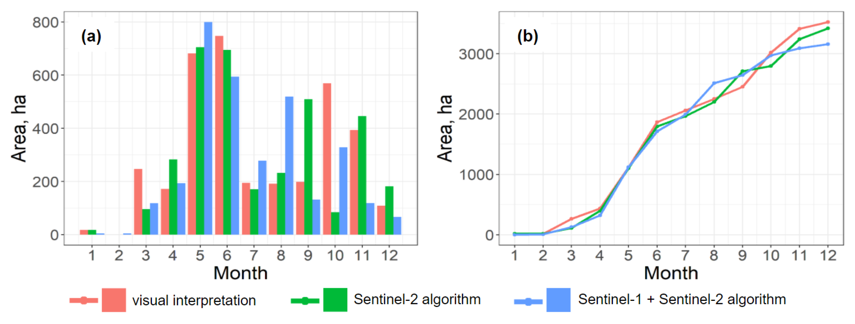
The best estimates of the sugarcane harvested areas per month have been obtained for the period of March–August 2018 when a cloudy pixel percentage was less than 45% of the image area.

To monitor harvest according to the SAR data, the coherence time series generated from Sentinel-1 IW SLC images have been used. Low coherence corresponds to the harvest period; the coherence grows sharply upon the harvest completion due to the bare soil or sparse vegetation. False responses of the SAR-based algorithm may be connected with the non-harvest field operations, that alter the signal reflection. To reduce the number of false responses, trends of the NDVI time series were used. It is supposed that the harvest is carried out on the decreasing NDVI trend. Note that in this case, the spatial resolution and/or periodicity of the optical sensors survey used for the construction of NDVI trends may be much lower than the ones used for detecting the harvest dates in the optical algorithm.

Accuracy of the harvest dates identification from Sentinel-1 SAR data is clearly inferior to the algorithm based on the Sentinel-2 optical data due to a considerably larger interval between surveys (12 days compared to 5 days). However, the SAR data may be used to clarify the harvest dates obtained according to the optical data and, in the long view, to specify the harvest dates during the periods of dense clouds.

Both algorithms have demonstrated the best performance while working with the fields where sugarcane is planted approximately simultaneously over the whole area. For the fields consisting of several sugarcane parcels at different stages of growth, it is recommended to perform preliminary segmentation into the homogeneous parcels.

References

1. OECD/FAO. OECD-FAO Agricultural Outlook 2019–2028; Technical Report; Paris/Food and Agriculture Organization of the United Nations: Rome, Italy, 2019. [Google Scholar]
2. Rahman, M.; Robson, A. Integrating Landsat-8 and Sentinel-2 Time Series Data for Yield Prediction of Sugarcane Crops at the Block Level. Remote Sens. 2020, 12, 1313. [Google Scholar] [CrossRef] [Green Version]
3. Stasolla, M.; Neyt, X. Applying Sentinel-1 time series analysis to sugarcane harvest detection. In Proceedings of the IGARSS 2019—2019 IEEE International Geoscience and Remote Sensing Symposium, Yokohama, Japan, 28 July–2 August 2019; pp. 1594–1597. [Google Scholar] [CrossRef]
4. De Ávila Ribeiro Junqueira, R.; Morabito, R. Modeling and solving a sugarcane harvest front scheduling problem. Int. J. Prod. Econ. 2019, 213, 150–160. [Google Scholar] [CrossRef]
5. De Oliveira Bordonal, R.; Carvalho, J.L.N.; Lal, R.; de Figueiredo, E.B.; de Oliveira, B.G.; Scala, N.L. Sustainability of sugarcane production in Brazil. A review. Agron. Sustain. Dev. 2018, 38, 23. [Google Scholar] [CrossRef] [Green Version]
6. Sungnul, S.; Pornprakun, W.; Prasattong, S.; Baitiang, C. Multi-Objective Mathematical Model for the Optimal Time to Harvest Sugarcane. Appl. Math. 2017, 8, 329–343. [Google Scholar] [CrossRef] [Green Version]
7. Molijn, R.; Iannini, L.; Rocha, J.; Hanssen, R. Sugarcane Productivity Mapping through C-Band and L-Band SAR and Optical Satellite Imagery. Remote Sens. 2019, 11, 1109. [Google Scholar] [CrossRef] [Green Version]
8. Aguiar, D.; Rudorff, B.; Silva, W.; Adami, M.; Mello, M. Remote Sensing Images in Support of Environmental Protocol: Monitoring the Sugarcane Harvest in São Paulo State, Brazil. Remote Sens. 2011, 3, 2682–2703. [Google Scholar] [CrossRef] [Green Version]
9. Momin, M.A.; Grift, T.; Valente, D.; Hansen, A. Sugarcane yield mapping based on vehicle tracking. Precis. Agric. 2018, 20, 896–910. [Google Scholar] [CrossRef]
10. Oré, G.; Alcântara, M.; Góes, J.; Oliveira, L.; Yepes, J.; Teruel, B.; Castro, V.; Bins, L.; Castro, F.; Luebeck, D.; et al. Crop Growth Monitoring with Drone-Borne DInSAR. Remote Sens. 2020, 12, 615. [Google Scholar] [CrossRef] [Green Version]
11. Luna, I.; Lobo, A. Mapping Crop Planting Quality in Sugarcane from UAV Imagery: A Pilot Study in Nicaragua. Remote Sens. 2016, 8, 500. [Google Scholar] [CrossRef] [Green Version]
12. Baghdadi, N.; Cresson, R.; Todoroff, P.; Moinet, S. Multitemporal Observations of Sugarcane by TerraSAR-X Images. Sensors 2010, 10, 8899–8919. [Google Scholar] [CrossRef] [Green Version]
13. Rouse, J.; Haas, R.; Scheel, J.; Deering, D. Monitoring Vegetation Systems in the Great Plains with ERTS. In Proceedings of the 3rd Earth Resource Technology Satellite (ERTS) Symposium, Washington, DC, USA, 10–14 December 1974; Volume 1, pp. 48–62. [Google Scholar]
14. Jordan, C.F. Derivation of leaf-area index from quality of light on the forest floor. Ecology 1969, 50, 663–666. [Google Scholar] [CrossRef]
15. Huete, A.; Didan, K.; Miura, T.; Rodriguez, E.P.; Gao, X.; Ferreira, L.G. Overview of the radiometric and biophysical performance of the MODIS vegetation indices. Remote Sens. Environ. 2002, 83, 195–213. [Google Scholar] [CrossRef]
16. Gao, B.-C. NDWI—A normalized difference water index for remote sensing of vegetation liquid water from space. Remote Sens. Environ. 1996, 58, 257–266. [Google Scholar] [CrossRef]
17. Zheng, B.; Campbell, J.B.; Serbin, G.; Galbraith, J.M. Remote sensing of crop residue and tillage practices: Present capabilities and future prospects. Soil Tillage Res. 2014, 138, 26–34. [Google Scholar] [CrossRef]
18. Daughtry, C.S.T.; Hunt, E.R.; Doraiswamy, P.C.; McMurtrey, J.E. Remote Sensing the Spatial Distribution of Crop Residues. Agron. J. 2005, 97, 864–871. [Google Scholar] [CrossRef]
19. Tuszynska, J.; Gatkowska, M.; Wrobel, K.; Jagiello, K. A pilot study on determining approximate date of crop harvest on the basis of Sentinel-2 satellite imagery. Geoinf. Issues 2018, 10, 65–77. [Google Scholar] [CrossRef]
20. Guarnieri, A.; Prati, C. SAR Interferometry: A “Quick and Dirty” Coherence Estimator for Data Browsing. IEEE Trans. Geosci. Remote Sens. 1997, 35, 660–669. [Google Scholar] [CrossRef] [Green Version]
21. Nasrallah, A.; Baghdadi, N.; Hajj, M.E.; Darwish, T.; Belhouchette, H.; Faour, G.; Darwich, S.; Mhawej, M. Sentinel-1 Data for Winter Wheat Phenology Monitoring and Mapping. Remote Sens. 2019, 11, 2228. [Google Scholar] [CrossRef] [Green Version]
22. Khabbazan, S.; Vermunt, P.; Steele-Dunne, S.; Arntz, L.R.; Marinetti, C.; van der Valk, D.; Iannini, L.; Molijn, R.; Westerdijk, K.; van der Sande, C. Crop Monitoring Using Sentinel-1 Data: A Case Study from The Netherlands. Remote Sens. 2019, 11, 1887. [Google Scholar] [CrossRef] [Green Version]
23. Harfenmeister, K.; Spengler, D.; Weltzien, C. Analyzing Temporal and Spatial Characteristics of Crop Parameters Using Sentinel-1 Backscatter Data. Remote Sens. 2019, 11, 1569. [Google Scholar] [CrossRef] [Green Version]
24. Kavats, O.; Khramov, D.; Sergieieva, K.; Vasyliev, V. Monitoring Harvesting by Time Series of Sentinel-1 SAR Data. Remote Sens. 2019, 11, 2496. [Google Scholar] [CrossRef] [Green Version]
25. Shang, J.; Liu, J.; Poncos, V.; Geng, X.; Qian, B.; Chen, Q.; Dong, T.; Macdonald, D.; Martin, T.; Kovacs, J.; et al. Detection of Crop Seeding and Harvest through Analysis of Time-Series Sentinel-1 Interferometric SAR Data. Remote Sens. 2020, 12, 1551. [Google Scholar] [CrossRef]
26. Bazzi, H.; Baghdadi, N.; Fayad, I.; Zribi, M.; Belhouchette, H.; Demarez, V. Near Real-Time Irrigation Detection at Plot Scale Using Sentinel-1 Data. Remote Sens. 2020, 12, 1456. [Google Scholar] [CrossRef]
27. Bazzi, H.; Baghdadi, N.; Ienco, D.; Hajj, M.E.; Zribi, M.; Belhouchette, H.; Escorihuelaand, M.J.; Demarez, V. Mapping Irrigated Areas Using Sentinel-1 Time Series in Catalonia, Spain. Remote Sens. 2019, 11, 1836. [Google Scholar] [CrossRef] [Green Version]
28. Virnodkar, S.; Pachghare, V.; Patil, V.; Jha, S. Application of Machine Learning on Remote Sensing Data for Sugarcane Crop Classification: A Review; Springer Nature Singapore Pte Ltd.: Singapore, 2020; Volume 2, pp. 539–555. [Google Scholar] [CrossRef]
29. Wang, M.; Liu, Z.; Baig, M.; Wang, Y.; Li, Y.; Chen, Y. Mapping sugarcane in complex landscapes by integrating multi-temporal Sentinel-2 images and machine learning algorithms. Land Use Policy 2019, 88, 104190. [Google Scholar] [CrossRef]
30. Schultz, B.; Immitzer, M.; Formaggio, A.; Sanches, I.; Luiz, A.; Atzberger, C. Self-Guided Segmentation and Classification of Multi-Temporal Landsat 8 Images for Crop Type Mapping in Southeastern Brazil. Remote Sens. 2015, 7, 14482–14508. [Google Scholar] [CrossRef] [Green Version]
31. Cevallos, J.C.; Villagomez, J.A.; Andryshchenko, I. Convolutional Neural Network in the Recognition of Spatial Images of Sugarcane Crops in the Troncal Region of the Coast of Ecuador. Procedia Comput. Sci. 2019, 150, 757–763. [Google Scholar] [CrossRef]
32. Mulianga, B.; Bégué, A.; Clouvel, P.; Todoroff, P. Mapping Cropping Practices of a Sugarcane-Based Cropping System in Kenya Using Remote Sensing. Remote Sens. 2015, 7, 14428–14444. [Google Scholar] [CrossRef] [Green Version]
33. Jiang, H.; Li, D.; Jing, W.; Xu, J.; Huang, J.; Yang, J.; Chen, S. Early Season Mapping of Sugarcane by Applying Machine Learning Algorithms to Sentinel-1A/2 Time Series Data: A Case Study in Zhanjiang City, China. Remote Sens. 2019, 11, 861. [Google Scholar] [CrossRef] [Green Version]
34. Li, H.; Yuan, X.; Han, Y.; Chen, J.; Chen, X. Monitoring of Sugarcane Crop based on Time Series of Sentinel-1 data. In 2019 SAR in Big Data Era (BIGSARDATA); IEEE: Piscataway, NJ, USA, 2019; p. 19045938. [Google Scholar] [CrossRef]
35. Zhao, H.; Chen, Z.; Jiang, H.; Jing, W.; Sun, L.; Feng, M. Evaluation of Three Deep Learning Models for Early Crop Classification Using Sentinel-1A Imagery Time Series—A Case Study in Zhanjiang, China. Remote Sens. 2019, 11, 2673. [Google Scholar] [CrossRef] [Green Version]
36. Santos, F.; Rabelo, S.; de Matod, M.; Eichler, P. (Eds.) Sugarcane Biorefinery, Technology and Perspectives; Elsevier: Amsterdam, The Netherlands, 2020; p. 289. [Google Scholar]
37. Nihei, T.; Hayashi, H.; Shirota, R. Characteristics of sugarcane production in the State of São Paulo, Brazil. Geosp. Space 2015, 8, 53–80. [Google Scholar] [CrossRef]
38. Land Viewer|EOS—EOS Data Analytics. Available online: https://eos.com/landviewer/ (accessed on 17 November 2020).
39. EOS Statistics API Documentation. Available online: https://doc-dev.eos.com/statistics.api/ (accessed on 17 November 2020).
40. Copernicus Open Access Hub. Available online: https://scihub.copernicus.eu/dhus/#/home (accessed on 17 November 2020).
41. Alaska Satellite Facility (ASF) VERTEX Service. Available online: https://search.asf.alaska.edu/#/ (accessed on 17 November 2020).
42. Sentinel Application Platform (SNAP). Available online: https://step.esa.int/main/toolboxes/snap/ (accessed on 17 November 2020).
43. Tukey, J. Exploratory Data Analysis; Addison-Wesley: Reading, MA, USA, 1977. [Google Scholar]
44. Zaitunah, A.; Samsuri; Ahmad, A.G.; Safitri, R. Normalized difference vegetation index (ndvi) analysis for land cover types using landsat 8 oli in besitang watershed, Indonesia. IOP Conf. Ser. Earth Environ. Sci. 2018, 126, 1–10. [Google Scholar] [CrossRef]
45. Kavats, A.; Khramov, D.; Sergieieva, K.; Vasyliev, V.; Kavats, Y. Geoinformation technology of agricultural monitoring using multi-temporal satellite imagery. In Proceedings of the ICAG 2018: 20th International Conference on Agriculture and Geoinformatics, Vienna, Austria, 14–15 June 2018. [Google Scholar]
46. Murugan, D.; Singh, D. Development of an Approach for Monitoring Sugarcane Harvested and Non-Harvested Conditions Using Time Series Sentinel-1 Data. In Proceedings of the IGARSS 2018—2018 IEEE International Geoscience and Remote Sensing Symposium, Valencia, Spain, 22–27 July 2018; pp. 5308–5311. [Google Scholar] [CrossRef]
47. Patel, J.; Oza, M. Deriving crop calendar using NDVI time-series. In Proceedings of the ISPRS Technical Commission VIII Symposium, Hyderabad, India, 9–12 December 2014; Volume XL-8, pp. 869–873. [Google Scholar] [CrossRef] [Green Version]
48. Marin, F.; Jones, J. Process-based simple model for simulating sugarcane growth and production. Sci. Agric. 2014, 71, 1–16. [Google Scholar] [CrossRef] [Green Version]
49. Ghazvinei, P.; Darvishi, H.; Mosavi, A.; Yusoff, K.b.W.; Alizamir, M.; Shamshirband, S.; Chau, K. Sugarcane growth prediction based on meteorological parameters using extreme learning machine and artificial neural network. Eng. Appl. Comput. Fluid Mech. 2018, 12, 738–749. [Google Scholar] [CrossRef] [Green Version]
50. Goltz, E.; Arcoverde, G.; de Aguiar, D.; Rudorff, B.; Maeda, E. Data mining by decision tree for object oriented classification of the sugar cane cut kinds. In Proceedings of the IGARSS 2009—2009 IEEE International Geoscience and Remote Sensing Symposium, Cape Town, South Africa, 12–17 July 2009; pp. V-405–V-408. [Google Scholar] [CrossRef]
51. Rahmad, C.; Rahutomo, F.; Gustalika, M.; Rahmah, I. Identification of sugarcane maturity scale based on RGB, Gabor feature extraction and Support Vector Machine. IOP Conf. Ser. Mater. Sci. Eng. 2018, 434, 012065. [Google Scholar] [CrossRef]
Figure 1. Location of the study area in the state of São Paulo (Brazil).
Remotesensing 12 04080 g001
Figure 2. Crop calendar of sugarcane in the state of São Paulo: Type A—winter planting (first harvest); Type B—summer planting (first harvest); Type C—ratooning (second to fifth harvest).
Remotesensing 12 04080 g002
Figure 3. Sentinel-1 and Sentinel-2 aquisition dates, 2018–2019.
Remotesensing 12 04080 g003
Figure 4. Example of a sugarcane parcel before (a,c) and after harvest (b,d) in natural colours (a,b) and NDVI (c,d).
Remotesensing 12 04080 g004
Figure 5. Example of the NDVI time series for a cell: (a) initial; (b) smoothened by the median filter; (c) smoothened by the modified median filter.
Remotesensing 12 04080 g005
Figure 6. Coherence time series: (a) type 1, harvest (red line): 11 August 2018; (b) type 2, harvest (red line): 12 June 2018.
Remotesensing 12 04080 g006
Figure 7. Stages of the NDVI time series trend construction for a cell: (a) the initial NDVI time series; (b) the series after filtration (1) with window width k = 3 ; (c) the series after averaging by the sliding median filter with window width k = 9 ; (d) the series after spline-smoothing.
Remotesensing 12 04080 g007
Figure 8. Comparison of the NDVI trends derive from Sentinel-2, Landsat-8, and MOD09Q1 (MODIS) data.
Remotesensing 12 04080 g008
Figure 9. Harvest dates: (1) identified by visual interpretation; (2) determined by the algorithm from the optical data; (3) coinciding harvest dates determined by the two mentioned methods.
Remotesensing 12 04080 g009
Figure 10. Quality indicators of harvest dates identification by month: (a) distribution of cloud fraction of Sentinel-2 images by month; (b) distribution of the coinciding harvest dates (optical algorithm and visual interpretation), omitted harvest dates, and dates of false response (optical algorithm) by month.
Remotesensing 12 04080 g010
Figure 11. The sugarcane areas harvested by month, identified by visual interpretation (lv), algorithm based on optical data (optic), algorithm based on Synthetic Aperture Radar (SAR) and optical data (sar): (a) absolute values; (b) accumulated values.
Remotesensing 12 04080 g011
Figure 12. Example of false response of the optical algorithm due to cloudiness in November (cid = 450). Actual harvest dates (red lines): 18 April 2018 and 4 December 2018; harvest dates according to the optical algorithm (blue lines): 18 April 2018 and 14 November 2018; harvest date according to the SAR algorithm (green line): 24 April 2018.
Remotesensing 12 04080 g012
Figure 13. (ac) Example of the cloudiness effect during the harvest period (November).
Remotesensing 12 04080 g013
Figure 14. Example of false response of the optical algorithm due to cloudiness in March and false response of the SAR algorithm due to field works in August (cid = 27). Actual harvest dates (red lines): 8 April 2018, 13 April 2018, and 14 November 2018; harvest dates according to the optical algorithm (blue lines): 29 March 2018, 13 April 2018, and 9 November 2018; harvest dates according to the SAR algorithm (green line): 12 April 2018 and 22 August 2018.
Remotesensing 12 04080 g014
Figure 15. (a,b) Example of the cloudiness effect during the harvest period (March).
Remotesensing 12 04080 g015
Figure 16. Example of false response of the optical algorithm due to cloudiness in June (cid = 226). Actual harvest date (red lines): 12 June 2018; harvest date according to the optical algorithm (blue lines): 2 June 2018; harvest date according to the SAR algorithm (green line): 23 June 2018.
Remotesensing 12 04080 g016
Figure 17. (a,b) Example of the cloudiness effect during the harvest period (June).
Remotesensing 12 04080 g017
Figure 18. Example of false response of the optical algorithm due to cloudiness in September and false response of the SAR algorithm due to field works in August (cid = 197). Actual harvest date (red lines): 15 October 2018; harvest date according to the optical algorithm (blue lines): 15 September 2018; harvest date according to the SAR algorithm (green line): 22 August 2018.
Remotesensing 12 04080 g018
Figure 19. Example of the harvest date omission by the SAR algorithm due to nonagricultural lands within the parcel (cid = 40). Actual harvest date (red lines): 12 June 2018; harvest date according to the optical algorithm (blue lines): 12 June 2018; harvest date according to the SAR algorithm (green line): 5 July 2018.
Remotesensing 12 04080 g019
Figure 20. Example of the sugarcane field fragment with the included nonagricultural lands (cid = 40) in natural colours (a) and NDVI (b).
Remotesensing 12 04080 g020
Figure 21. Example of the harvest date omission by the SAR algorithm due to nonagricultural lands within the parcel (cid = 163). Actual harvest dates (red lines): 14 March 2018, 12 June 2018, 2 July 2018, and 7 July 2018; harvest dates according to the optical algorithm (blue lines): 7 July 2018 and 15 September 2018; harvest date according to the SAR algorithm (green line): 5 July 2018.
Remotesensing 12 04080 g021
Figure 22. Example of the parcel with nonagricultural vegetation (cid = 163): (a) before harvest; (b) partial harvest; (c) completely harvested parcel.
Remotesensing 12 04080 g022
Figure 23. Example of the parcel with inclusions of a neighbouring field (cid = 516): (a) the most of the parcel is not harvested; (b) both parts are harvested.
Remotesensing 12 04080 g023
Figure 24. Example of the harvest date omission and false response of the SAR algorithm for a nonhomogeneous parcel (cid = 29). Actual harvest dates (red lines): 8 April 2018, 13 April 2018, and 10 October 2018, 7 July 2018; harvest dates according to the optical algorithm (blue lines): 29 March 2018 and 15 September 2018; harvest dates according to the SAR algorithm (green line): 11 June 2018, 22 August 2018, and 21 October 2018.
Remotesensing 12 04080 g024
Figure 25. (a,b) Example of a nonhomogeneous parcel (cid = 29).
Remotesensing 12 04080 g025