Abstract
Through Global Navigation Satellite System (GNSS) occultation measurement, the global ionosphere and atmosphere can be observed. When the navigation satellites’ signal passes through the lower atmosphere, the rapid change of the atmospheric refractive index gradient will cause serious multipath phenomena in radio wave propagation. Atmospheric doppler frequency shift and amplitude signal fluctuations increase drastically. Due to the attenuation of signal amplitude and the rapid change of the Doppler frequency, the general phase locked loop (PLL) cannot work properly. Hence, a more stable tracking technology is needed to track the occultation signal passing through the lower atmosphere. In this paper, a mountain-top based radio occultation experiment is performed, where we employ an open-loop receiver and remove the navigation bits by the internal demodulation. In the process of the experiment, we adopt the open-loop tracking technique and there is no feedback between the observed signal and the control model. Specifically, taking the pseudo-range and doppler information from models as input, three key parameters, i.e., accurate code phase, carrier doppler and code doppler, can be obtained, and furthermore, the accurate accumulation is determined by them. For the full open-loop occultation data, a closed-loop observation assisted strategy is presented to compare the tracking results between open-loop and closed-loop occultation data. Through the compared results, we can determine whether the initial phase has been reversed or not, and obtain the high consistency corrected open-loop data that can be directly used for subsequent atmospheric parameters inversion. To verify the effect of open-loop tracking and open-loop inversion, we used the company’s self-developed occult receiver system for verification. The company’s self-developed occult receiver system supports Global Position System (GPS)/Beidou satellites constellation (BD, the 2nd and 3rd generations) dual systems. We have verified GPS and BD open-loop tracking and inversion, carried out in a three-week mountain-based experiment. We used closed-loop and open-loop strategies to track and capture the same navigation star to detect its acquisition effect. Finally, we counted the results of a week (we only listed the GPS data; BD’s effect is similar). The experimental results show that the open-loop has expanded the signal-cut-off angle by nearly 20% under the condition of counting all angles, while the open-loop has increased the signal-cut-off angle value by nearly 89% when only calculating the negative angle. Finally, the atmosphere profiles retrieved from observations in open-loop tracking mode are evaluated with the local observations of temperature, humidity and pressure provided by the Beijing Meteorological Bureau, and it is concluded that the error of open-loop tracking method is within ~4% in MSER (mean square error of relative error), which meets the accuracy of its applications (<5%, in MSER).
1. Introduction
Global Navigation Satellite System (GNSS) occultation measurement is a meteorological remote sensing technology, which utilizes occultation phenomenon between GNSS navigation constellation and low earth orbit (LEO) satellites in its orbit to measure the earth’s ionosphere and atmosphere [1,2,3]. By installing GNSS occultation antennas on the LEO satellites, it is possible to obtain the atmospheric refractive index, temperature, pressure from the earth’s surface to 40 km and the ionospheric electronic distortion rate from ~60 km to the orbital height of the occultation LEO satellite [4,5]. Atmospheric detection is of great significance for the weather forecast, scientific research and military application [6,7,8].
The occultation signal from GNSS satellites has low and negative elevation angles [9,10,11]. Many approaches to data processing in the presence of multipath propagation (methods based on Fourier Integral Operators, like Canonical Transform, Full Spectrum Inversion and Phase Matching) can be found in references [12,13,14,15,16,17,18]. When the occultation signal passes through the lower atmosphere, especially the equatorial low latitude area, serious multipath phenomena appear in radio waves due to the rapid change of atmospheric refractive index gradient [19,20,21]. The fluctuation of atmospheric doppler frequency shifts and amplitude signal increases sharply, and the spectrum of occultation signal expands [6,7,8]. Due to the attenuation of signal amplitude and the rapid change of doppler frequency, the general phase locked loop (PLL) cannot work normally.
Until recently, two very important challenges remained outstanding: (1) the ability to record and retrieve rising occultations; and (2) the ability to penetrate the lowest 2 km in the tropical troposphere routinely (for rising or setting occultations) without introducing tracking errors. These challenges have largely been overcome by the use of open-loop (OL) tracking implemented in the GPS receivers onboard the SAC-C satellite, and later Constellation Observing System for Meteorology, Ionosphere and Climate (COSMIC) [22]. Closed-loop tracking is a method of tracking the carrier frequency and code frequency of satellite launches in real time, through the adjustment of the software’s own loop route. The OL tracking technique is different from the traditional closed-loop tracking, in that there is no feedback between the observation signal and the control model. Meanwhile, signal tracking in the OL mode uses the predicted Doppler model and pseudo-range model to track the full signal, and has the ability to track stably [22,23,24].
A mountain-based occultation experiment for three weeks in Wuling Mountain of Hebei Province is planned and implemented, with the following works to be carried out: 1. A hardware and software system supporting Global Position System (GPS)/Beidou satellites constellation (BD, the 2nd and 3rd generations) dual-mode occultation being developed for full OL tracking technology’s verification; 2. An open-loop data processing method assisted with closed-loop observations, which is proposed to solve the problem to determine the initial sign of the recovered phase; 3. In the mountain-based occultation experiment, the robustness of the hardware and software systems using OL technology to track L1C/GPS and B1/BD signals being verified; and 4. The atmosphere profiles retrieved from observations in open-loop tracking mode being evaluated with the local observations of temperature, humidity and pressure provided by the Beijing Meteorological Bureau.
2. Open-Loop Tracking and Inversion Algorithm
2.1. Open-Loop Tracking Algorithm
OL tracking uses the predicted Doppler and pseudo-range models to track the signal [25,26]. The difference between the OL and the traditional PLL is that there is no feedback between the observation signal and the control model, but only the model control signal is used, so it will not be affected by the change of the signal [27,28]. It can track full information of phases (the effects of motion, atmospheric multipath, etc.), and can detect rising occultation events more conveniently [29,30].
The mountain-based OL tracking algorithm is different from the spaceborne OL tracking algorithm in terms of the model Doppler and pseudo range. In the satellite OL tracking module, we employ the international reference atmospheric model CIRA86-Q for pseudo-range/Doppler prediction. The mountain-based OL tracking algorithm is mainly used to verify the correctness of OL tracking, not to verify the correctness of the Doppler and pseudo range model. In the verification process of the mountain-based OL tracking algorithm, we assume that the Doppler and pseudo-range are mainly changed by the movement of GNSS satellites, while the effects of the atmosphere and the ionosphere are small. In the mountain-based test, the position and speed of the navigation satellite can be obtained through the ephemeris. The geometric distance of between the station and the satellite at an occultation and the Doppler of motion obtained based on the velocity of that satellite are used as the output of the pseudo-range/Doppler model to narrow the phase search range in full OL tracking. The chip array of the mountain-based occultation receiver is expanded to ensure that the phase delay caused by the atmosphere is within the chips’ range.
2.2. Open Open-Loop Data Processing
In the OL mode, the phase used to retrieve for atmosphere profiles can be expressed as sum of the modeled phase (MP) and the recovered phase (RP). The MP is obtained from the occultation geometry and climate models. The RP is restored from observations of the In-Phase(I)/Quadra-Phase(Q) components through three steps: frequency reduction conversion; NDM removal; and adjacent phase connection [28,31,32,33,34]. The ways to eliminate the influence of NDM in the OL mode are the internal and external methods, and the biggest difference between them is that the external mode requires GPS bit data. Due to geographical restrictions, however, only about 70% of the COSMIC occultation data has corresponding GPS bit data [31,32,33,34]. Due to a lack of information in determining the initial sign of RP, there may be a different sign between the initial I/Q components and the real phase, which will negatively correct the MP. We adopt the strategy of the full OL data recovery process, assisted with closed-loop observations to avoid the above-mentioned problems. Through MPs adding or subtracting RPs, we can obtain two series phases, named corrected phases A/B(CPA/CPB). We use the correlation between the mountain-based closed-loop observation data of an elevation angle above 3 degrees and CPA/CPB to determine the initial sign of RP, and obtain a high-consistency corrected OL phase for subsequent atmospheric parameter inversion.
2.3. Mountain-Based Atmospheric Retrieval Algorithm
The GNSS signal can generally be expressed as follows:
where c is the speed of light, and is the observed phase of the transmitter (s) and receiver (r) of the i-th frequency at time (t). is the geometric distance between transmitter (s) and receiver (r) at time t. , are the clock difference of the transmitter (s) and receiver (r) at time (t), respectively. is the local multipath error [35,36]; is the residual phase. is the ambiguity of the whole cycle. The excess phase of transmitter s and receiver (r) of the i-th frequency at time (t) is generally defined as the sum of neutral atmospheric delay and ionospheric delay [36,37,38,39,40].
Based on Internet GNSS Servers (IGS) products and low-orbit satellite precision orbit determination products, it is possible to obtain a sufficiently accurate distance from the navigation satellite transmitter to the low-orbit satellite receiver and its clock difference . The local multipath error can be ignored in mountain-based occultation. The receiver clock error can generally be eliminated by selecting a higher altitude navigation star as a reference and applying the satellites’ phase difference. As a result, high-precision excess phase observations of the occultation can be obtained, which only include the influence of the ionosphere and atmosphere through the path. In the process of spaceborne neutral atmosphere inversion, the combination of different frequency point bending angle sequences can better eliminate the ionospheric influence. In extracting the excess phase, only the ionospheric influence of the reference star can be eliminated. In the mountain-based atmospheric occultation inversion, the atmospheric state information from the ground to the top of the mountain can be obtained through the relationship between the impact height observed by the positive and negative altitude angle. As shown in Figure 1, observation of negative elevation angle (light and dark green thick line, bending angle is ) can be regarded as the Abel integral (light green thick line) and positive elevation angle (light blue thick line, bending angle is ) from the top to the impact height, namely [39,40,41,42]:
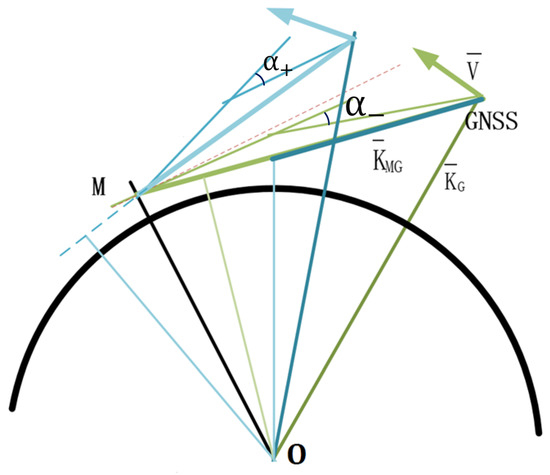
Figure 1.
Schematic diagram of mountain base inversion. M stands for the top of the mountain, where the antenna and receiver are installed, and Global Navigation Satellite System (GNSS) stands for the navigation satellite we want to receive, that is, the navigation satellite that generates the occultation event.
Let
then the refractive index n of the impact height ( is the peak refractive index, is the maximum impact height of the occultation) is:
Thus, the refractive index profile from the ground to the top of the mountain can be obtained from the mountain-based occultation data [42,43].
In the above process, the influence of the atmosphere or ionosphere on the observation data above the top of the mountain can be eliminated in the process of searching for the symmetrical impact height and its combination. Therefore, when the clock error of the mountaintop receiver is eliminated by the reference star, only the ionospheric influence of the reference star needs to be eliminated, while the mountain-based occultation observation data does not need to consider its influence on the excess phase. Even with only single frequency observation data, the refractive index inversion results from the ground to the top of the mountain can be obtained.
As shown in Figure 2, according to the geometric relationship of the mountain-based occultation, Excess phase and Doppler of transmitter (s) and receiver (r) at frequency (i) at time (t), The impact height (the superscript and subscripts and the time label are omitted here) and the bending angle have the following relationship [44]:
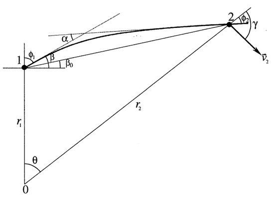
Figure 2.
Geometry diagram of mountain base occultation. Coordinate point 1 represents the site of the mountain base test, at the top of Wuling Mountain. Coordinate point 2 represents the navigation satellite at an occultation event.
Among these, is the frequency of frequency point , and are the signal incident angle and the center distance of the receiver and transmitter, respectively. is the angle between the vector from the Earth’s center to the receiver and the transmitter. is the occultation velocity, and is the angle between the occultation velocity and the vector from the Earth’s center to the transmitter.
3. Mountain-Based Test Results
The mountain-based occultation experiment is from 25 August to 8 September 2020. The site of the observation is the top of Wuling Mountain, the main peak of the Yanshan Mountains (located in Chengde, Hebei Province, 117.48 degrees east longitude, 40.60 degrees north latitude, and 2118 m above sea level), and the occultation antenna is deployed on the roof of Dingfeng Hotel. As shown in Figure 3 and Figure 4, the south side of the mountain is empty. Our occultation antenna (right side) is installed on the top of the building and placed facing south, and the receiver is installed inside the room.
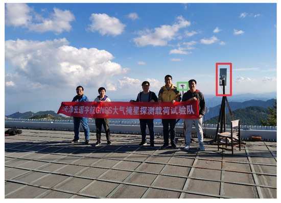
Figure 3.
Mountain-based location, behind our experiment team is the bottom of the mountain. Our occultation antenna (the part marked in red in the picture) is mounted on a tripod and placed facing south, and our positioning antenna (the part marked in green in the picture) is also installed on the tripod. On the tripod, place it towards the zenith. The south side of the mountain is empty, which is conducive to our experiments.
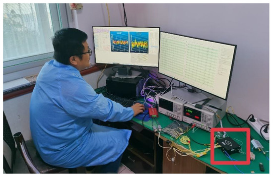
Figure 4.
Installation drawing of equipment room, our equipment is installed indoors, as shown in the figure (red marking part) and verified by the company’s self-researched occultation detector. It has the characteristics of small volume and low power consumption. It is also the equipment we will use in satellite networking in the future. It is placed on the anti-static pad, and ground treatment is also carried out to prevent the occurrence of static electricity and lightning strike events on the mountain.
The GNSS occultation receiver system used for testing is developed by Tianjin Yunyao Aerospace Technology Co., Ltd, which is compatible with GPS/BD systems.
3.1. Analysis of GPS and BD Open-Loop Tracking Results
The I and Q components of the signal have different characteristics in OL and closed-loop tracking. In the tracking process, the phases of the OL flipped by NDM and error from the OL predict model in the form of a trigonometric function on the I/Q components, which can be seen from Figure 5. The phases of the closed-loop are of huge value, with signal flipped in the I component, and the Q component is signal noise. The closed-loop tracking can detect the phase or frequency difference between the locally reproduced carrier and the received carrier through the phase detector or frequency discriminator in the carrier loop. Then, the phase alignment of the local PN code and the received code can be continuously adjusted through the code loop discriminator, so as to obtain the highest self-phase correlation peak value.
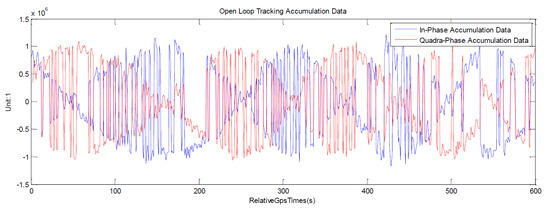
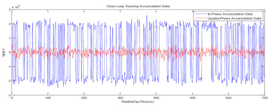
Figure 5.
Real-time results of open-loop (OL)/closed-loop signal components of In-Phase (I, in blue line) and Quadra-Phase (Q, in red line). The abscissa is relative time in second, and the ordinate represents the components’ value. The top plane shows the characteristics of OL tracking mode that extreme values alternately appear in I and Q components; the bottom plane shows the characteristics of the closed-loop tracking mode that extreme values appeared in the I component.
This paper analyzes the mountain-based occultation observations from full OL tracking mode in the following ways. First, using the excess phase obtained from the observation data in the closed-loop tracking mode as the reference, the continuity and duration of the excess phases obtained in the OL tracking verifies that the full OL tracking mode of GPS and BD are more robust than the closed-loop tracking mode. Second, the refractivity profiles retrieved from observations in the OL and closed-loop tracking modes are compared to verify their consistency.
We selected (part of) the data on September 7 for analysis. The data include rising and falling occultations. As shown in Figure 6 and Figure 7, excess phases retrieved from observations of L1C/GPS in OL/closed-loop tracking mode are compared, as well as that of B1/BD. Figure 8 shows the difference of the excess phase retrieved from observations of L1C/GPS and B1/BD in OL/closed-loop tracking mode, which are within 0.2 m. From Figure 6, Figure 7 and Figure 8, the following can be concluded:
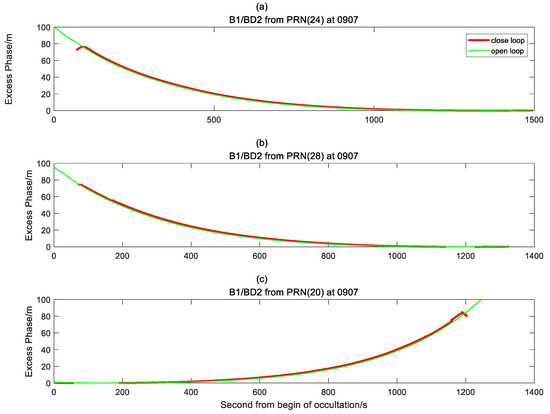
Figure 6.
Excess phases retrieved from observations of B1/BD in OL/closed-loop tracking mode. Red/green lines represent the phases in closed-loop/OL tracking mode, respectively. (a) C24/BD occultation; (b) C28/BD occultation; and (c) C20/BD occultation.
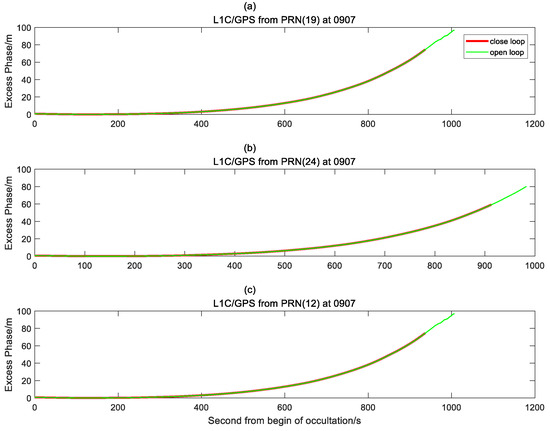
Figure 7.
Excess phase retrieved from observations of L1C/GPS in OL/closed-loop tracking mode. Red/green lines represent the phases in closed-loop/OL tracking mode, respectively. (a) G19/GPS occultation; (b) G24/GPS occultation; and (c) G12/GPS occultation.
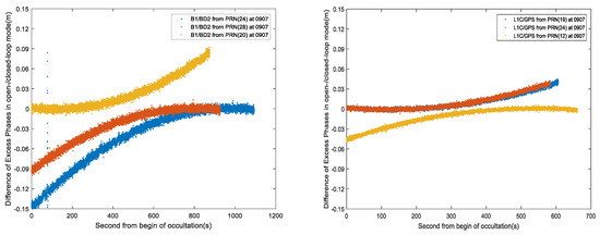
Figure 8.
Difference of excess phase retrieved from observations of B1/BD and L1C/GPS in OL/closed-loop tracking mode. Left panel, B1/BD; Right panel, L1C/GPS.
- (1)
- OL tracking time is longer than closed-loop, that is, for low-angle occultation events, OL has a better tracking effect.
- (2)
- The mountain-based occultation data can only detect the peak height and below. It can be seen from Figure 6 and Figure 7 that compared to closed-loop tracking, the OL tracking can capture a lower height, and has the same result as the closed-loop tracking. Hence, the continuity of the OL is relatively robust. From the curve, we can see that the excess phase changes obtained by GPS and BD are relatively robust, and there is no deterioration in signal capture quality due to drastic changes in the signal.
- (3)
- The OL tracking effect of GPS and BD are similar, and both have a greater improvement compared to closed-loop tracking.
Figure 9 and Figure 10 show the refractivity profiles obtained from the observations of L1C/GPS and B1/BD in the OL/closed-loop tracking mode, respectively. In these figures, the refractivity profiles obtained from the observations in the OL/closed-loop mode in the overlap height have the same trend along altitude. The minimum height of refractivity profiles obtained from L1C/GPS signal in OL mode are about 0.4 km, and that of the closed-loop mode are about 1.6 km. The minimum height of refractivity profiles from B1/BD signal in OL mode are about 1.2 km, and that of closed-loop mode are between 1.3–1.5 km. Figure 11 visualizes the difference of refractivity profiles retrieved from observations of B1/BD and L1C/GPS in OL/closed-loop mode, from which it is concluded that: 1. the bias of the refractivity retrieved from observations of L1C/GPS and B1/BD in OL/closed-loop mode is within 1N; and 2. The trend of the refractivity profiles retrieved from observations of L1C/GPS in OL/closed-loop mode is slightly better than the result of B1/BD.
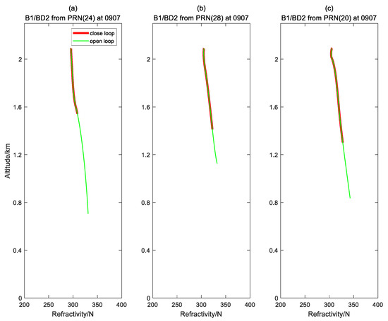
Figure 9.
Refractivity profiles retrieved from observations of B1/BD in OL/closed-loop tracking mode, respectively. Red/green lines represent results in closed-/OL mode tracking, respectively. (a) C24/BD Occultation; (b) G28/BD Occultation; and (c) C12/BD Occultation.
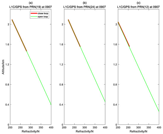
Figure 10.
Refractivity profiles retrieved from observations of L1C/GPS in OL/closed-loop tracking mode. Red/green lines represent results in closed-/OL mode tracking, respectively. (a) G19/GPS Occultation; (b) G24/GPS Occultation; and (c) G12/GPS Occultation.
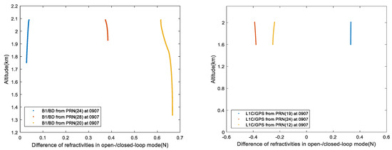
Figure 11.
Difference of refractivity profiles retrieved from observations of B1/BD and L1C/GPS in OL/closed-loop tracking mode. Left panel, B1/BD; Right panel, L1C/GPS.
3.2. Comparison of Closed-Loop Tracking and Open-Loop Tracking
In order to verify the effectiveness of the OL tracking algorithm, the comparison of the OL and closed-loop methods is used for verification, and the OL and closed-loop channels are used to capture and track the same satellite. Compare the start capture angle and end capture angle of the two to verify the capture effect. We selected 7 days of observation data for statistics, and the selected data are shown in Table 1:

Table 1.
List of the closed-loop initial pitch angle (CLIPA), closed-loop end pitch angle (CLEPA), open-loop initial pitch angle (OLIPA), open-loop end pitch angle (OLEPA) and start/end azimuth (SA, EA) from selected occultation events.
From Table 1, it can be seen that the full OL tracking method can effectively capture occultation events at lower angles. As shown in Table 1, observations from an occultation of GPS (PRN 30) at 1 September 2020 0:10:43 UT showed that its OL end pitch angle reached −1.87 deg, which is 0.88 deg smaller than its closed-loop end pitch angle. At low elevation angles, it is difficult to track in the closed-loop strategy stably, and problems such as drastic changes in the signal-to-noise ratio and loss of signal lock will occur. The fully OL tracking method effectively solves the above problems.
We have made statistics on all the data to evaluate the effect of OL tracking. One calculation method is to calculate the angles of the whole occultation tracking, and mark it as strategy A; the other is to calculate the negative angles of the occultation tracking, and mark it as strategy B. For strategy A or B, the way to evaluate the capture capability of the OL/closed loop tracking, and the effect of OL tracking are:
in which , are the initial pitch angle and end pitch angle, respectively; , are values to evaluate the capture capability of the OL/closed-loop tracking with strategy A or B; and , are the effects of OL tracking evaluated with strategy A or B. According to observations from Table 1, the result of accumulating the seven-day data are:
A = 19.35%, B = 88.54%.
The results show that in the case of counting all angles, the OL improves the capture angle range of data volume by nearly 20%, and when only the negative angle is calculated, the OL improves the capture angle value by nearly 89%. The mountain-based situation is different from the onboard situation. We will continue to verify the actual capture effect in the future. However, there is no doubt that the fully OL capture method greatly improves the capture effect. We make the difference between the OL angle and the closed-loop angle (only the negative angle is counted), and the result is shown in Figure 12. There is no specific coupling relationship between OL tracking and closed-loop tracking, but the overall effect is better than closed-loop. The reason why there is no specific coupling relationship is due to the difference between the two capture methods. The angle difference is mainly concentrated between 1° and 1.2°.
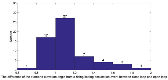
Figure 12.
Histogram of the difference of the start/end elevation angle from a rising/setting occultation event between closed-loop and OL. Because the top height of the mountain is about 2 km, the minimum elevation angle value is generally about −3° in OL mode, and the difference is mainly concentrated between 0.8° and 1.2°.
3.3. Comparison of Open-Loop Tracking Inversion Results and Meteorological Observations
The atmosphere profiles retrieved from observations in OL tracking mode are evaluated with the local observations of temperature, humidity and pressure provided by the Beijing Meteorological Bureau.
The atmospheric refractive index of the observation point can be calculated by temperature, relative humidity and pressure data, which is used to verify the accuracy of the inversion of the mountain-based experimental data. The calculation method is as follows [45,46,47,48]:
Using the temperature data of the analysis field to calculate the corresponding saturated vapor pressure:
In the above formula, is the saturated vapor pressure at the corresponding temperature, and is the temperature in Celsius. The constant . There is the following relationship between actual vapor pressure , saturated vapor pressure and relative humidity:
Finally, the approximate relationship between refractive index and atmospheric parameters can be used to obtain the atmospheric refractive index:
In the above formula, is the refractive index of the atmosphere, is the total atmospheric pressure (), is the water vapor pressure () and is the atmospheric temperature .
For each sounding profile data, find the matching occultation profile (one or more), and interpolate them to the altitude points with a distance of 0.05 km. Calculate the standard deviation of the average refractive index deviation and the absolute refractive index deviation within the height range covered by both the occultation and the sounding profile as the evaluation standard.
The results are shown in the following Table 2 (partially):
Table 2.
The relative refractive index deviation standard deviation statics of each atmosphere profile.
It can be seen from the results that the BIAS/MSER of the OL tracking method is within 0.5% and 4%, respectively, which meet the accuracy of its applications (<0.5%, in BIAS; <5%, in MSER).
4. Conclusions
1. We designed and developed the occultation equipment that supports the GPS/BD systems, and tested its performance based on mountain-based experiments. It is concluded that B1/BD observation data can obtain atmospheric retrieval accuracy similar to L1C/GPS observation. Since the 2nd and 3rd generations of the BD constellations have more than 50 satellites in orbit, the equipment will be deployed on low-orbit satellites in the future to obtain more occultation observations.
2. Traditional OL processing relies on external data (GPS bit) to determine the initial sign of the RP. We use internal processing to recover the phase of the full OL tracking observation data for mountain-based occultation inversion. Due to the lack of external data, it is difficult to determine the initial RP sign. We use the correlation between the mountain-based closed-loop observation data of elevation angle above 3 degrees and the RP data to determine the initial sign of RP, and accomplish the full OL data recovery process based on closed-loop observations automatically.
3. To determine the full OL tracking and capturing effect, we have performed statistics on the data for 7 consecutive days. The statistical results showed that in the case of counting all angles, the OL improves the capture angle value by nearly 20%, and when only the negative angle is calculated, the OL improves the capture angle value by nearly 89%. The full-open-loop capture mode greatly improves the capture effect, and there is no specific coupling relationship between OL tracking and closed-loop tracking, but the overall effect is better than closed-loop. The reason why there is no specific coupling relationship is due to the difference between the two capture methods.
4. The atmosphere profiles retrieved from observations in OL tracking mode are evaluated with the local observations of temperature, humidity and pressure provided by the Beijing Meteorological Bureau. It can be concluded that the error of the OL tracking method is within ~4% in the mean square error of relative error (MSER), which meets the accuracy of its applications (<5%, in MSER).
Author Contributions
Conceptualization, F.L., L.K., N.F., M.W., C.H. and Z.W.; methodology, F.L., L.K. and N.F.; formal analysis, L.K.; investigation, L.K.; data curation, F.L.; writing—original draft preparation, F.L.; writing—review and editing, F.L. and L.K.; data analysis and discrimination, F.L., N.F. and L.K.; supervision, F.L.; project administration, L.K.; and funding acquisition, F.L. All authors have read and agreed to the published version of the manuscript.
Funding
This work was supported in part by the National Natural Science Foundation of China under Grant Nos. 61520106002 and 61731003.
Acknowledgments
The validation data was provided by Beijing Meteorological Administration, and the experiments team of Tianjin Yunyao Aerospace Technology Co., Ltd. We also thank reviewers for their suggestions on improvement in the article.
Conflicts of Interest
The authors declare no conflict of interest.
References
- Wu, D.L. Ionospheric S4 Scintillations from GNSS Radio Occultation (RO) at Slant Path. Remote Sens. 2020, 12, 2373. [Google Scholar] [CrossRef]
- Pilch Kedzierski, R.; Matthes, K.; Bumke, K. New insights into Rossby wave packet properties in the extratropical UTLS using GNSS radio occultations. Atmos. Chem. Phys. Discuss. 2020. [Google Scholar] [CrossRef]
- Cardellach, E.; Oliveras, S.; Rius, A.; Tomás, S.; Ao, C.O.; Franklin, G.W.; Iijima, B.A.; Kuang, D.; Meehan, T.K.; Padullés, R.; et al. Sensing heavy precipitation with GNSS polarimetric radio occultations. Geophys. Res. Lett. 2019, 46, 1024–1031. [Google Scholar] [CrossRef]
- Ershov, B.G. Radiation-chemical decomposition of seawater: The appearance and accumulation of oxygen in the Earth’s atmosphere. Radiat. Phys. Chem. 2020, 168, 108530. [Google Scholar] [CrossRef]
- Hordyniec, P.; Huang, C.Y.; Liu, C.Y.; Rohm, W.; Chen, S.Y. GNSS radio occultation profiles in the neutral atmosphere from inversion of excess phase data. Terr. Atmos. Ocean. Sci. 2019, 30. [Google Scholar] [CrossRef]
- Wallace, J.M.; Chang, C.P. Spectrum analysis of large-scale wave disturbances in the tropical lower troposphere. J. Atmos. Sci. 1969, 26, 1010–1025. [Google Scholar] [CrossRef]
- Fritts, D.C.; Tsuda, T.; Kato, S.; Sato, T.; Fukao, S. Observational evidence of a saturated gravity wave spectrum in the troposphere and lower stratosphere. J. Atmos. Sci. 1988, 45, 1741–1759. [Google Scholar] [CrossRef][Green Version]
- Ruston, B.; Healy, S. Forecast Impact of FORMOSAT-7/COSMIC-2 GNSS Radio Occultation Measurements. Atmos. Sci. Lett. 2020, e1019. [Google Scholar] [CrossRef]
- Beyerle, G.; Zus, F. Open-loop GPS signal tracking at low elevation angles from a ground-based observation site. Atmos. Meas. Tech. 2017, 10, 359. [Google Scholar] [CrossRef]
- Collett, I.; Morton, Y.T.; Wang, Y.; Breitsch, B. Characterization and mitigation of interference between GNSS radio occultation and reflectometry signals for low-altitude occultations. Navig. J. Inst. Navig. 2020, 67, 537–546. [Google Scholar] [CrossRef]
- Mendillo, M.; Huang, C.L.; Pi, X.; Rishbeth, H.; Meier, R. The global ionospheric asymmetry in total electron content. J. Atmos. Solar-Terr. Phys. 2005, 67, 1377–1387. [Google Scholar] [CrossRef]
- Sokolovskiy, S.V. Modeling and inverting radio occultation signals in the moist troposphere. Radio Sci. 2001, 36, 441–458. [Google Scholar] [CrossRef]
- Sokolovskiy, S.V. Effect of super refraction on inversions of radio occultation signals in the lower troposphere. Radio Sci. 2003, 38, 1058. [Google Scholar] [CrossRef]
- Jensen, A.S.; Lohmann, M.S.; Benzon, H.-H.; Nielsen, A.S. Full Spectrum Inversion of radio occultation signals. Radio Sci. 2003, 38, 1040. [Google Scholar] [CrossRef]
- Jensen, A.S.; Lohmann, M.S.; Nielsen, A.S.; Benzon, H.-H. Geometrical optics phase matching of radio occultation signals. Radio Sci. 2004, 39, RS3009. [Google Scholar] [CrossRef]
- Gorbunov, M.E. Radioholographic Methods for Processing Radio Occultation Data in Multipath Regions; Danish Meteorological Institute: Copenhagen, Denmark, 2001. [Google Scholar]
- Gorbunov, M.E. Canonical transform method for processing radio occultation data in lower troposphere. Radio Sci. 2002, 37, 1076. [Google Scholar] [CrossRef]
- Gorbunov, M.E. Radio-holographic analysis of Microlab-1 radio occultation data in the lower troposphere. J. Geophys. Res. 2002, 107, 4156. [Google Scholar] [CrossRef]
- Kan, V.; Gorbunov, M.E.; Shmakov, A.V.; Sofieva, V.F. Reconstruction of the Internal-Wave Parameters in the Atmosphere from Signal Amplitude Fluctuations in a Radio-Occultation Experiment. Izv. Atmos. Ocean. Phys. 2020, 56, 435–447. [Google Scholar] [CrossRef]
- Kan, V.; Gorbunov, M.E.; Sofieva, V.F. Fluctuations of radio occultation signals in sounding the Earth’s atmosphere. Atmos. Meas. Tech. 2018, 11, 663–680. [Google Scholar] [CrossRef]
- Sokolovskiy, S.; Schreiner, W.; Zeng, Z.; Hunt, D.; Lin, Y.C.; Kuo, Y.H. Observation, analysis, and modeling of deep radio occultation signals: Effects of tropospheric ducts and interfering signals. Radio Sci. 2014, 49, 954–970. [Google Scholar] [CrossRef]
- Ao, C.O.; Hajj, G.A.; Meehan, T.K.; Dong, D. Rising and setting GPS occultations by use of open-loop tracking. J. Geophys. Res. 2009, 114, D04101. [Google Scholar] [CrossRef]
- Chase, S.M.; Schwartz, A.B.; Kass, R.E. Bias, optimal linear estimation, and the differences between open-loop simulation and closed-loop performance of spiking-based brain–computer interface algorithms. Neural Netw. 2009, 22, 1203–1213. [Google Scholar] [CrossRef]
- Borovic, B.; Liu, A.Q.; Popa, D.; Cai, H.; Lewis, F.L. Open-loop versus closed-loop control of MEMS devices: Choices and issues. J. Micromech. Microeng. 2005, 15, 1917. [Google Scholar] [CrossRef]
- Lohmann, M.S. Analysis of Global Positioning System (GPS) radio occultation measurement errors based on Satellite de Aplicaciones Cientificas-c (SAC-C) GPS radio occultation data recorded in open-loop and phase-locked-loop mode. J. Geophys. Res. Atmos. 2007, 112, 115. [Google Scholar] [CrossRef]
- Alexandru, C. A novel open-loop tracking strategy for photovoltaic systems. Sci. World J. 2013, 2013, 205396. [Google Scholar] [CrossRef]
- Sokolovskiy, S.; Schreiner, W.; Rocken, C.; Hunt, D. Optimal Noise Filtering for the Ionospheric Correction of GPS Radio Occultation Signals. J. Atmos. Ocean. Technol. 2009, 26, 1398–1403. [Google Scholar] [CrossRef]
- Rahman, M.; Shukla, S.K.; Prasad, K.N.; Ovejero, C.M.; Pati, B.K.; Tripathi, A.; Singh, A.; Srivastava, A.K.; Gonzalez-Zorn, B. Prevalence and molecular characterisation of New Delhi metallo-β-lactamases NDM-1, NDM-5, NDM-6 and NDM-7 in multidrug-resistant Enterobacteriaceae from India. Int. J. Antimicrob. Agents 2014, 44, 30–37. [Google Scholar] [CrossRef]
- Jin, T.; Yuan, H.; Ling, K.V.; Qin, H.; Kang, J. Differential Kalman Filter Design for GNSS Open Loop Tracking. Remote Sens. 2020, 12, 812. [Google Scholar] [CrossRef]
- Zhang, L.; Yang, X.; Dong, Q.; Dong, J.; Liu, X.; Pan, L. Research on Enhancement Scheme of GPS Occultation Open-Loop Tracking Strategy. In China Satellite Navigation Conference 2020 Proceedings; Springer: Singapore, 2020; pp. 576–584. [Google Scholar] [CrossRef]
- Sokolovskiy, S.V. Tracking tropospheric radio occultation signals from low Earth orbit. Radio Sci. 2001, 36, 483–498. [Google Scholar] [CrossRef]
- Sokolovskiy, S.; Rocken, C.; Hunt, D.; Schreiner, W.; Johnson, J.; Masters, D.; Esterhuizen, S. GPS profiling of the lower troposphere from space: Inversion and demodulation of the open-loop radio occultation signals. Geophys. Res. Lett. 2006, 33. [Google Scholar] [CrossRef]
- Wu, J.; Tang, X.; Li, Z.; Li, C.; Wang, F. Cascaded interference and multipath suppression method using array antenna for GNSS receiver. IEEE Access 2019, 7, 69274–69282. [Google Scholar] [CrossRef]
- Sokolovskiy, S.; Rocken, C.; Schreiner, W.; Hunt, D.; Johnson, J. Postprocessing of L1 GPS radio occultation signals recorded in open-loop mode. Radio Sci. 2009, 44, RS2002. [Google Scholar] [CrossRef]
- Vagle, N.; Broumandan, A.; Jafarnia-Jahromi, A.; Lachapelle, G. Performance analysis of GNSS multipath mitigation using antenna arrays. J. Glob. Position. Syst. 2016, 14, 4. [Google Scholar] [CrossRef]
- Hegarty, C.J. GNSS signals—An overview. In Proceedings of the 2012 IEEE International Frequency Control Symposium Proceedings, Baltimore, MD, USA, 21–24 May 2012. [Google Scholar]
- Appleget, A.; Bartone, C. A Consolidated GNSS Multipath Analysis Considering Modern GNSS Signals, Antenna, Installation, and Boundary Conditions. In Proceedings of the 32nd International Technical Meeting of the Satellite Division of The Institute of Navigation (ION GNSS), Miami, FL, USA, 16–20 September 2019; pp. 2855–2869. [Google Scholar] [CrossRef]
- Humphreys, T.E.; Ledvina, B.M.; Bencze, W.J.; Galusha, B.T.; Cohen, C.E. Assimilating GNSS Signals to Improve Accuracy, Robustness, and Resistance to Signal Interference. U.S. Patent Application No. 12/889,242, 24 March 2011. [Google Scholar]
- Yao, Z.; Lu, M.; Feng, Z.M. Quadrature multiplexed BOC modulation for interoperable GNSS signals. Electron. Lett. 2010, 46, 1234–1236. [Google Scholar] [CrossRef]
- Alhussein, F.; Liu, H. An Efficient Method for Multipath Mitigation Applicable to BOC Signals in GNSS. In Proceedings of the 2019 15th International Wireless Communications & Mobile Computing Conference (IWCMC), Tangier, Morocco, 24–28 June 2019; pp. 793–798. [Google Scholar] [CrossRef]
- Wood, V.T.; Brown, R.A.; Vasiloff, S.V. Improved detection using negative elevation angles for mountaintop WSR-88Ds. Part II: Simulations of the three radars covering Utah. Weather Forecast. 2003, 18, 393–403. [Google Scholar] [CrossRef]
- Hu, X.; Wu, X.C.; Gong, X.Y.; Xiao, C.Y.; Zhang, X.X.; Fu, Y.; Du, X.Y.; Li, H.; Fang, Z.Y.; Xia, Q.; et al. An introduction of mountain-based GPS radio occultation experiments in China. Adv. Space Res. 2008, 42, 1723–1729. [Google Scholar] [CrossRef]
- Cremers, C.J.; Birkebak, R.C. Application of the Abel integral equation to spectrographic data. Appl. Opt. 1996, 5, 1057–1064. [Google Scholar] [CrossRef]
- Morton, Y.; Bourne, H.; Taylor, S.; Xu, D.; Yang, R.; van Graas, F.; Pujara, N. Keynote: Mountain-top radio occultation with multi-GNSS signals: Experiment and preliminary results. In Proceedings of the ION 2017 Pacific PNT Meeting, Honolulu, HI, USA, 1–4 May 2017; pp. 490–499. [Google Scholar] [CrossRef]
- Wu, X.C.; Hu, X.; Gong, X.Y. Comparison of refractivity obtained with mountain-based GPS radio occultation and radiosonde. Prog. Geophys. 2008, 23, 1149–1155. [Google Scholar]
- Gong, X.Y.; Hu, X.; Wu, X.C. Comparison between mountain-based GPS occultation observations and results from automatic weather station. Prog. Geophys. 2008, 23, 1480–1486. [Google Scholar]
- Hu, X.; Zhang, X.X.; Wu, X.C.; Xiao, C.Y.; Zeng, Z.; Gong, X.Y. Mountain-based GPS observations of occultation and its inversion theory. Chin. J. Geophys. 2006, 49, 22–27. [Google Scholar] [CrossRef]
- Fu, E.J.; Zhang, K.F.; Marion, K.Y. Assessing COSMIC GPS radio occultation derived atmospheric parameters using Australian radiosonde network data. Procedia Earth Planet. Sci. 2009, 1, 1054–1059. [Google Scholar] [CrossRef]
Publisher’s Note: MDPI stays neutral with regard to jurisdictional claims in published maps and institutional affiliations. |
© 2020 by the authors. Licensee MDPI, Basel, Switzerland. This article is an open access article distributed under the terms and conditions of the Creative Commons Attribution (CC BY) license (http://creativecommons.org/licenses/by/4.0/).