Parameter Optimization for Uncertainty Reduction and Simulation Improvement of Hydrological Modeling

Abstract

Hydrological modeling has experienced rapid development and played a significant role in water resource management in recent decades. However, modeling uncertainties, which are propagated throughout model runs, may affect the credibility of simulation results and mislead management decisions. Therefore, analyzing and reducing uncertainty is of significant importance in providing greater confidence in hydrological simulations. To reduce and quantify parameter uncertainty, in this study, we attempted to introduce additional remotely sensed data (such as evapotranspiration (ET)) into a common parameter estimation procedure that uses observed streamflow only. We undertook a case study of an application of the Soil Water Assessment Tool in the Guijiang River Basin (GRB) in China. We also compared the effects of different combinations of parameter estimation algorithms (e.g., Sequential Uncertainty Fitting version 2, particle swarm optimization) on reduction in parameter uncertainty and improvement in modeling precision improvement. The results indicated that combining Sequential Uncertainty Fitting version 2 (SUFI-2) and particle swarm optimization (PSO) can substantially reduce the modeling uncertainty (reduction in the R-factor from 0.9 to 0.1) in terms of the convergence of parameter ranges and the aggregation of parameters, in addition to iterative optimization. Furthermore, the combined approaches ensured the rationality of the parameters’ physical meanings and reduced the complexity of the model calibration procedure. We also found the simulation accuracy of ET improved substantially after adding remotely sensed ET data. The parameter ranges and optimal parameter sets obtained by multi-objective calibration (using streamflow plus ET) were more reasonable and the Nash–Sutcliffe coefficient (NSE) improved more rapidly using multiple objectives, indicating a more efficient parameter optimization procedure. Overall, the selected combined approach with multiple objectives can help reduce modeling uncertainty and attain a reliable hydrological simulation. The presented procedure can be applied to any hydrological model.

1. Introduction

Improving the reliability of hydrological modeling simulation by reducing modeling uncertainty to support water resource planning and management is an ongoing goal for the hydrological community [1,2,3]. Due to the development of distributed hydrological models, hydrological research has progressed significantly. However, the equifinality resulting from different parameter sets indicates that there uncertainties remain in the modeling processes [4,5]. Such uncertainty may affect simulation accuracy and even result in misleading assessments, compromising water resource management [6,7]. Controlling the range of parameters and adding additional constraints can help reduce such modeling uncertainty [8,9,10,11]. Therefore, improving the accuracy and credibility of hydrological modeling by constraining the parameters is of high potential interest in the hydrological community [12,13].

The source of uncertainty in hydrological models can be generally classified into three categories: input and calibration data uncertainty (e.g., climate, underlying surface, and streamflow data), structural uncertainty (e.g., process descriptions and equations), and parameter uncertainty [14,15,16,17]. Of these, parameter uncertainties are common but can be easily controlled to improve model performance and credibility, which has been a major focus in the modeling uncertainty field [10,18,19,20]. Several approaches were also developed for parameter optimization and uncertainty analysis, of which generalized likelihood uncertainty estimation (GLUE) [21], Sequential Uncertainty Fitting version 2 (SUFI-2) [22], and particle swarm optimization (PSO) [23] are the most popular. GLUE is easy to use in model calibration but results in greater uncertainty [24,25]. The SUFI-2 method can more efficiently provide satisfactory simulations, but requires additional iterations and manual adjustment of parameter ranges after each iteration [18,26]. For example, Qiao [9] found the uncertainty indicator (i.e., R-factor) decreased dramatically using the four-stage SUFI-2 method to narrow the range of parameters. PSO can automatically process the parameter optimization and achieve rapid convergence of parameters [25]. These studies are valuable in the understanding of modeling uncertainties and associated analysis methods.

In most cases, it is difficult to obtain parameter values directly from field measurements and thus parameter optimization with a target hydrological variable may be needed [11,27,28]. Generally, streamflow observations are used for model calibration because they are readily available and linked to various hydrological processes [3,4]. Model calibration with streamflow only may result in acceptable streamflow simulation but incorrect representation of other processes, such as soil moisture, evapotranspiration (ET), and groundwater recharge. Previous studies found that multi-objective calibration is an effective means of improving simulations [20,29,30,31]. Compared to calibration with a single streamflow gaging station, using multiple streamflow gaging stations can help reduce uncertainty and improve simulation accuracy [32,33]. Zhang [34] calibrated Soil and Water Assessment Tool (SWAT) with streamflow data from three gages using four different optimization methods (PSO, GLUE, SUFI-2, and parameter solution). Chien [35] calibrated SWAT using SUFI-2 with multi-site streamflow observations and found that different regions have unique buffering capabilities in response to climate change. Additionally, for better simulation of the hydrological processes, other variables, such as ET, soil moisture, and groundwater, can be added for model calibration [4,20,29,34]. Rajib [3] found the simulation performance improved noticeably when calibrating with additional Moderate-resolution Imaging Spectroradiometer (MODIS) ET data. Qiao [9] found that the SWAT model performance can be significantly improved by introducing both groundwater storage and streamflow into the calibration procedure. Researchers also considered that the predictability of hydrological models can be significantly improved when jointly calibrating with streamflow and satellite-based ET data [3,27]. However, other reports have also indicated that calibration involving multiple variables may lead to worse model performance in streamflow simulation compared to streamflow-only calibration [20]. Clearly, many studies have verified that multi-objective (i.e., using more than one observed variable) calibration can be an efficient means to improve the performance of the model, particularly in the examination of multiple processes rather than streamflow only. However, few studies have examined the impacts of multi-objective calibration on modeling uncertainty, which is the motivation of the current study.

The overall goal of this study was to provide a feasible and efficient means for parameter optimization, and reducing and quantifying uncertainty. Thus, we applied two common optimization and uncertainty analysis approaches (SUFI-2 and PSO) and their combinations for model inversion. Each approach and combination was applied with single-objective and multi-objective calibrations to analyze the effect of different model constraints on modeling accuracy and uncertainty reduction.

2. Materials and Methods

2.1. Study Area

The Guijiang River is a tributary of the Xijiang River in the Pearl River Basin, located in southern China, and originates in the north of Maoer Mountain and flows southeast through Guangxi province with a length of 426 km. The drainage area of the Guijiang River Basin (GRB) (23°–25° N, 110°–111° E, 18,606 km², Figure 1) is 19,288 km². The GRB lies in the subtropical monsoon climate zone, with an uneven characteristic distribution of precipitation concentrated mostly from April to June [36,37]. The annual precipitation ranges from 1600 to 1800 mm, and the annual mean temperature (T) ranges from 18 °C in the upstream to 21 °C in the downstream [37]. Topographically, the altitude decreases from the highest in the northwest to the lowest in the southeast. Land uses mainly include forest (61%), cropland (19%), shrubland (9%), grass (7%), urban (3%), and water (1%). The main soil types are Acrisols (60%), Luvisols (14%), Anthrosols (10%), Alisols (8%), and Cambisols (6%), with other soil types accounting for less than 2% (Figure 1).

2.2. Model Description

The SWAT model was developed by the Agricultural Research Service of the United States Department of Agriculture (USDA-ARS) to predict impacts of climate and land use/management changes on water, sediment, and agricultural chemical yields [1,38,39,40]. This physically based distributed model has been widely applied for the estimation of watershed issues under climate change and human activities at watershed scales. The main outputs of SWAT are streamflow, ET, soil water, groundwater, sediment load, and nitrogen and phosphorus loads [41,42,43,44]. More details can be found in the SWAT input/output documentation [45]. SWAT is considered to be one of the best tested models in the field of hydrological simulation and has been widely used globally. In particular, the model is open-source and can facilitate users’ modifications to meet their specific needs. Therefore, SWAT was selected and modified technically, in this study, to adapt it for ET calibration, using SWAT Calibration and Uncertainty Programs (SWAT-CUP). SWAT-CUP is an integrated program for sensitivity analysis, calibration, validation, and uncertainty analysis of SWAT models.

2.3. Model Input and Setup

The SWAT model requires inputs on weather and topography data. A digital elevation model (DEM) was obtained from NASA’s Shuttle Radar Topography Mission (SRTM V3.0) with 3 arc second (~90 m) resolution [46]. The land use (2015) and soil type maps with 1 km resolution were obtained from the Ecological and Environmental Science Data Center for West China (http://westdc.westgis.ac.cn). Daily meteorological data of five weather stations (1951–2016) were obtained from the National Meteorological Information Center (http://data.cma.cn), including precipitation (P), maximum and minimum air temperature, relative humidity (RH), wind speed (WS), and sunshine duration (SD). The solar radiation (SR) was calculated based on SD and latitude [41]. The Geographic Information System (GIS) interface, ArcSWAT (version 2012), was used to delineate the watershed, resulting in 86 sub-basins and 2141 HRUs (Hydrologic Response Units).

2.4. Model Calibration/Validation and Uncertainty Analysis

SWAT-CUP was employed in this study for model calibration and uncertainty quantification. We used two hydrological variables, namely, streamflow from two stations (Zhaoping and Jingnan as shown in Figure 1) and ET of the entire GRB for model calibration and validation. Monthly streamflow data at these two gaging stations were obtained from the local hydrological department, and the remotely sensed ET (MOIDS16A2 ET) was provided by NASA Land Processes Distributed Active Archive Center (LP DAAC, https://modis.gsfc.nasa.gov/data/dataprod/mod16.php), covering the period from 2000 to 2014.

In this study, the SWAT model was examined with streamflow and MODIS ET using a 13 year (1998–2010) record for calibration and another 5 year (2011–2015) period for validation (Figure 2). The influences of initial conditions were minimized using a 5 year (1993–1997) warm-up period [40]. Based on a review of literature related to SWAT calibration and our own experience [20,43,46,47,48,49,50,51], we selected seven important parameters for optimization (this step can be implemented using parameter sensitivity analysis for a customized project), and their adjustment modes and initial ranges are defined in

Table 1. Calibrated parameters of the SWAT model for the Guijiang River Basin.

Parameter names	Description	Initial Range
r_CN2.mgt	SCS curve number at moisture condition II	[−0.2, 0.2]
v_ALPHA_BF.gw	Base flow recession constant	[0.001, 0.05]
v_CH_K2.rte	Effective hydraulic conductivity in main channel alluvium	[0, 150]
r_SOL_AWC.sol	Available water capacity of the soil layer	[−0.2, 0.2]
r_SOL_K.sol	Saturated hydraulic conductivity	[−0.2, 0.2]
v_ESCO.hru	Soil evaporation compensation factor	[0, 1]
v_SURLAG.bsn	Surface runoff lag time	[0.1, 4]

Note: “v_” means the existing parameter value is to be replaced by a given value, “r_” means an existing parameter value is multiplied by (1+ a given value).

. These seven parameters can affect the hydrologic responses of surface runoff subsurface lateral flow and channel routing procedures in SWAT simulations. As stated in Table 1, CN2, SOL_AWC, and SOL_K were adjusted using a relative adjustment approach (i.e., multiplying the initial value by a coefficient (1+ a given value)) to maintain their spatial variation, with adjustment ranges between −20% and 20% [20,33,52]. ALPHA_BF, CH_K2, ESCO, and SURLAG were replaced by a new given value, with adjustment ranges based on prior knowledge of the GRB and a review of existing publications [15,30,53]. Before the scenario design, we compared the results of 1000, 2000, 3000, and 5000 model runs and found that the results showed no significant difference after 2000 runs. Hence, we used SUFI-2, PSO, and combined SUFI-2–PSO approaches for uncertainty quantification and reduction, with a total of 2000 model runs for each approach. Below is a brief introduction to these approaches.

2.4.1. SUFI-2

SUFI-2 is a Bayesian-based optimized algorithm [54] that quantifies the uncertainties using sequential and fitting processes. In the parameter identification process, a sensitivity matrix and Hessian matrix are calculated to update and narrow the parameter ranges. A short step-by-step description of SUFI-2 is as follows:

Step 1: Define an objective function. We selected the commonly used Nash–Sutcliffe coefficient (NSE) [55] (Equation (A1) in Appendix A.1) as the objective function in this study. R² (Equation (A2) in Appendix A.2) and percentage of bias (PBIAS) (Equation (A3) in Appendix A.3) were also used for evaluating model performance.

Step 2: Set the initial ranges for the selected parameters which are to be calibrated (Table 1). Several sets of parameters are generated by Latin hypercube sampling (LHS) that are used for model simulations. Then, the NSE for each variable is calculated to assess the model performance.

Step 3: Evaluate each sampling round by a series of measures [22]. The sensitivity matrix J, the Hessian matrix H, and the parameter covariance matrix C are calculated as:

$$J_{ij}=\frac{\mathsf{∆}{g}_i}{\mathsf{∆}{b}_j}i=1,\dots ,C_2^n,j=1,\dots ,m$$

(1)

$$H=J^{T}J$$

(2)

$$C=S_g^2{\left(J^{T}J\right)}^{-1}$$

(3)

where $b$ is the parameter vector and $g$ is the objective function, $C_2^n$ is the number of all combinations of the two simulations, m is the number of parameters,$S_g^2$ is the variance of the objective function values, i.e., NSEs, in this study.

Step 4: Quantify the uncertainty. The 95% prediction uncertainty (95PPU) [22], R-factor, and P-factor are used to illustrate the fitting degree and uncertainty.

The average width of 95PPU is calculated as:

$$\overline{d_Q}=\frac{1}{K}{\displaystyle \sum }_{l=1}^K\left(Q_U-Q_L\right)$$

(4)

As in Equation (1), $K$ is the number of observations. The subscripts “U” and “L” mean upper (97.5th) and lower (2.5th) boundary of 95PPU, respectively.

R-factor is the relative width of 95PPU and P-factor is the percentage of observations bracketed by the 95PPU [9,56]. These are calculated by the following equations:

$$R-factor=\frac{\overline{d_Q}}{{\sigma }_Q}$$

(5)

$$P-factor=\frac{k_c}{K}$$

(6)

where ${\sigma }_Q$ is the standard deviation of variable $Q$ and $k_c$ is the number of values covered by 95PPU.

Step 5: Update the parameter ranges for further iteration.

2.4.2. PSO

PSO is a kind of self-adaptive random algorithm based on a group hunting strategy [57,58]. The particles are initially randomized in the given ranges followed by an iterative search for optima. Two optima, pbest and gbest, are defined for the update of particles. Pbest is the best solution for a particle, and gbest is the global optimum obtained by any particle in the population [59].

The PSO framework in SWAT-CUP is as follows:

Step 1: Initialize all particles. In SWAT-CUP, users define the number of simulations (particles) S and iterations I. Then, S sets of parameter values are generated randomly.

Step 2: Calculate the fitness value NSE, which is also the objective function in SUFI-2, obtain pbest and gbest, and compare them with previous values. If the present value is better, then reset the best value.

Step 3: Calculate the velocity and position of each particle for the next iteration.

Step 4: Implement Step 2 using the updated particles for further iterations until the number of iterations reaches I.

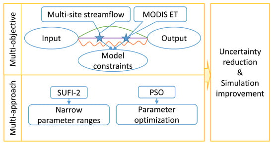
2.4.3. SUFI-2 and PSO Combination and Scenario Setting

SUFI-2 enables precise position of parameter ranges that are usually narrower than the last iteration. However, the posterior parameter ranges need to be checked and manually adjusted by users for the next iteration. SWAT-CUP can automatically provide a set of parameter ranges after one iteration. Users can use the recommended ranges or adjust them to ensure their physical meaning for the next iteration. PSO is an effective automatic global optimization method in which the optimization efficiency decreases with the increase in simulation times. This means PSO can achieve a satisfactory simulation with less calibration time. To improve optimization efficiency and decrease modeling uncertainty, we combined SUFI-2 and PSO in different arrangements as listed in

Table 2. Scenario setting of different approaches.

Approach Number	Approach	Scenario Code	Description
No.1	SUFI-2 2000	1-R	Run SUFI-2 2000 times, calibrate with streamflow only
		1-RE	Run SUFI-2 2000 times, calibrate with streamflow and ET
No.2	PSO 2000	2-R	Run PSO 2000 times, calibrate with streamflow only
		2-RE	Run PSO 2000 times, calibrate with streamflow and ET
No.3	SUFI-2 1000+PSO 1000	3-R	Run SUFI-2 1000 times, then PSO 1000 times, calibrate with streamflow only
		3-RE	Run SUFI-2 1000 times, then PSO 1000 times, calibrate with streamflow and ET
No.4	SUFI-2 500*2+PSO 1000	4-R	Run SUFI-2 500 times for two rounds, then PSO 1000 times, calibrate with streamflow only
		4-RE	Run SUFI-2 500 times for two rounds, then PSO 1000 times, calibrate with streamflow and ET
No.5	SUFI-2 500*3+PSO 500	5-R	Run SUFI-2 500 times for three rounds, then PSO 500 times, calibrate with streamflow only
		5-RE	Run SUFI-2 500 times for three rounds, then PSO 500 times, calibrate with streamflow and ET
No.6	SUFI-2 500*4	6-R	Run SUFI-2 500 times for four rounds, calibrate with streamflow only
		6-RE	Run SUFI-2 500 times for four rounds, calibrate with streamflow and ET

Note: “R” means calibration using streamflow data only, “RE’ means calibration using streamflow and ET simultaneously, and the number of “*” represents the number of manual operations.

. The primary principle of the combination approach is to obtain posterior parameter ranges from SUFI-2, followed by optimizing parameters using PSO. Approaches No.1, No.2, and No.6 (using SUFI-2 or PSO only) were set as the reference to compare the effects of different combined approaches. Approaches No.3, No.4, and No.5 were the different combinations of SUFI-2 and PSO algorithms.

Each approach mentioned above was used for streamflow calibration only (R) and streamflow plus ET calibration (RE), leading to twelve scenarios in total (scenario codes are listed in Table 2).

2.4.4. Evaluation Criteria

• For sensitivity analysis, the parameter with the greatest absolute value of t-stat and smaller p-value was regarded to be more sensitive. The t-stat measured the parameter sensitivity ranks, and a greater absolute value indicated a more sensitive parameter. The p-value represented the significance of sensitivity; p ≤ 0.05 means the parameters were significantly sensitive to the model simulations, and there was no statistical significance when the p-value $>$ 0.05.
• We used “*” to represent the operational complexity, and each “*” means manually adjusting parameter ranges once (Table 4).
• The values of parameters should be in reasonable ranges to ensure the reasonability of a parameter.
• NSE was set as the objective function to quantify the goodness of fit. Moreover, R² and PBIAS were used to describe the parallelism and deviation between simulations and observations.
• We set 0.8 as the threshold to determine behavioral (that is NSE $\ge$ 0.8) and non-behavioral (NSE $<$ 0.8) simulations [2,60]. A higher proportion of behavioral simulations (PBS) meant that the parameter ranges were more reasonable.
• The width of 95PPU indicated modeling uncertainty, and a narrower band means less uncertainty.
• R-factor is the relative width of 95PPU, and P-factor is the percentage of observation data points bracketed by the 95PPU. The ideal situation is that R-factor is close to 0, and P-factor is close to 1 [52], indicating the lowest uncertainty and highest accuracy.

3. Results

3.1. Parameter Sensitivity

The sensitivity analysis results of seven selected parameters under different scenarios (see scenario code in Table 2) are listed in

Table 3. Ranks of parameter sensitivity in different approaches.

	1-R			1-RE			2-R			2-RE
	Rank	t-Stat	p-Value	Rank	t-Stat	p-Value	Rank	t-Stat	p-Value	Rank	t-Stat	p-Value
CH_K2	1	−166.22	0.00	1	−93.63	0.00	1	−26.17	0.00	1	−38.32	0.00
CN2	2	61.50	0.00	2	26.27	0.00	2	16.43	0.00	2	17.93	0.00
ALPHA_BF	3	18.33	0.00	4	10.73	0.00	3	11.09	0.00	3	6.76	0.00
SOL_K	4	−3.24	0.00	5	−1.76	0.08	7	−0.93	0.35	5	−2.72	0.01
ESCO	5	2.89	0.00	3	−11.11	0.00	4	7.46	0.00	4	5.80	0.00
SURLAG	6	−1.29	0.20	6	−0.60	0.55	5	3.10	0.00	7	−0.65	0.52
SOL_AWC	7	−0.54	0.59	7	0.26	0.79	6	−1.09	0.28	6	−1.86	0.06
	3-R			3-RE			4-R			4-RE
	Rank	t-Stat	p-Value	Rank	t-Stat	p-Value	Rank	t-Stat	p-Value	Rank	t-Stat	p-Value
CH_K2	1	−20.48	0.00	1	−23.74	0.00	2	−8.78	0.00	2	−22.35	0.00
CN2	3	10.32	0.00	3	9.05	0.00	4	3.27	0.00	3	11.74	0.00
ALPHA_BF	2	13.77	0.00	2	16.50	0.00	3	4.90	0.00	1	24.54	0.00
SOL_K	7	0.71	0.48	4	−3.78	0.00	7	0.81	0.42	7	0.49	0.62
ESCO	4	10.31	0.00	5	3.00	0.00	1	11.01	0.00	4	4.65	0.00
SURLAG	6	−1.61	0.11	7	−1.03	0.30	5	2.81	0.00	5	−1.62	0.11
SOL_AWC	5	1.99	0.05	6	−1.03	0.30	6	0.83	0.40	6	1.42	0.16
	5-R			5-RE			6-R			6-RE
	Rank	t-Stat	p-Value	Rank	t-Stat	p-Value	Rank	t-Stat	p-Value	Rank	t-Stat	p-Value
CH_K2	7	−1.21	0.23	3	−3.90	0.00	1	−16.11	0.00	2	−9.79	0.00
CN2	3	−2.47	0.01	5	1.96	0.05	4	2.79	0.01	6	0.81	0.42
ALPHA_BF	2	4.72	0.00	1	17.81	0.00	2	5.70	0.00	3	4.32	0.00
SOL_K	5	2.09	0.04	4	−2.21	0.03	5	−1.51	0.13	4	−1.49	0.14
ESCO	1	10.14	0.00	2	−8.67	0.00	3	−2.87	0.00	1	−21.68	0.00
SURLAG	4	−2.26	0.02	6	−1.88	0.06	6	−0.90	0.37	7	−0.79	0.43
SOL_AWC	6	−1.69	0.09	7	−0.08	0.93	7	0.81	0.42	5	1.43	0.15

, and the ranking (1 to 7) is based on the absolute value of the t-stat for each approach. CH_K2 was the most sensitive parameter in this study with the largest t-stat for most of the scenarios. SOL_AWC ranked last among the seven parameters in this sensitivity analysis. In the initial iteration, all parameters showed relatively higher sensitivity index. As the iteration increased, however, the parameter range narrowed and the sensitivity index declined. This showed that the parameter sensitivity was dependent on the allowable range of a parameter, and could be lower when it approached the optimal value.

3.2. Model Performance

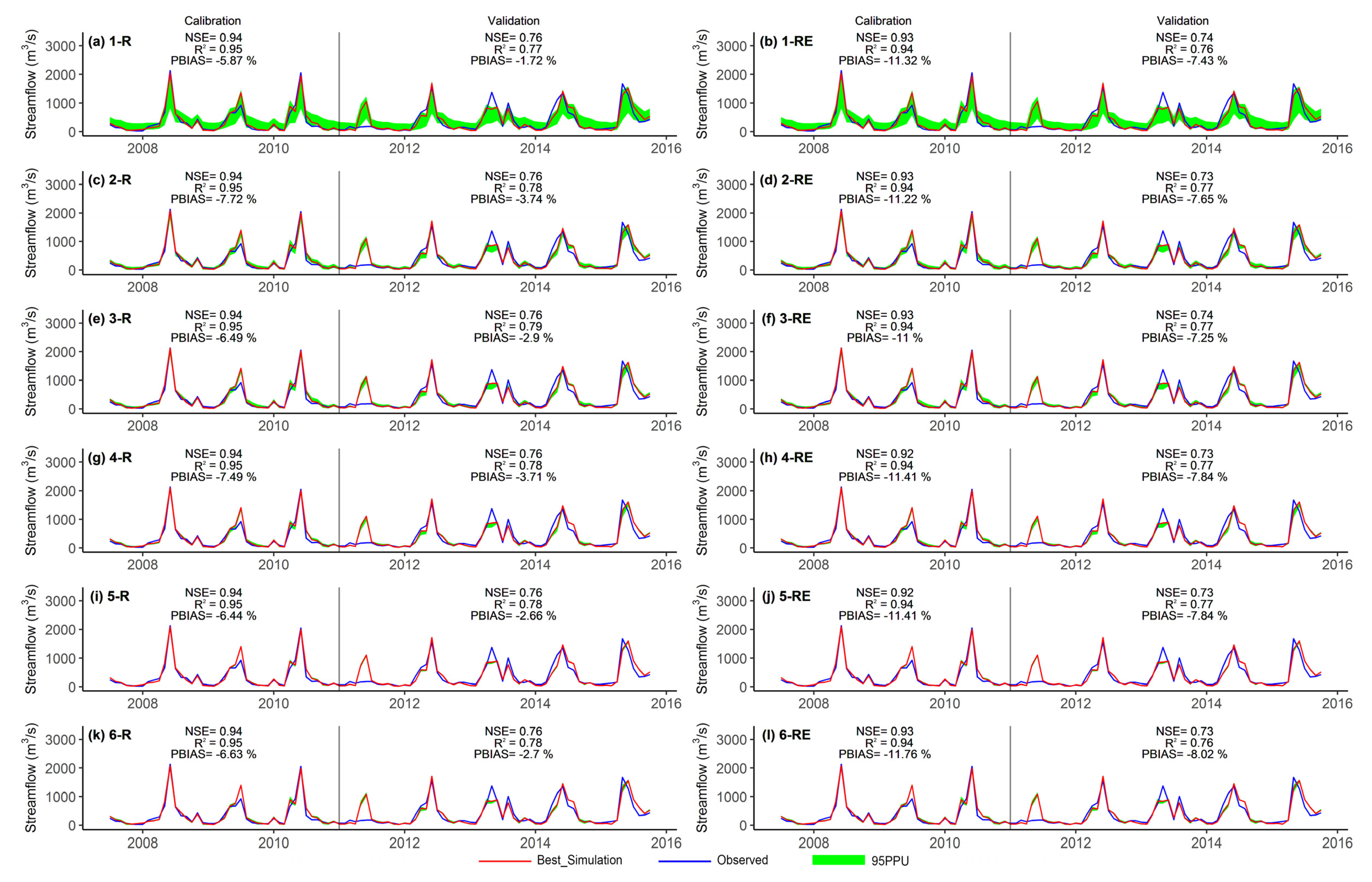
Model performance in simulating streamflow and ET was evaluated in this study.

Table 4. Complexity, model performance, and uncertainty of different scenarios.

Scenario Code	Complexity	NSE (Optimal)	R-Factor	P-Factor
1-R	*	0.854	0.925	0.840
1-RE	*	0.826	0.883	0.760
2-R	*	0.857	0.335	0.705
2-RE	*	0.828	0.300	0.633
3-R	**	0.862	0.270	0.630
3-RE	**	0.830	0.233	0.573
4-R	***	0.860	0.185	0.535
4-RE	***	0.829	0.177	0.503
5-R	****	0.859	0.085	0.375
5-RE	****	0.829	0.100	0.407
6-R	****	0.857	0.160	0.480
6-RE	****	0.827	0.197	0.517

Note: each “*” indicates manually adjusting the parameter ranges once.

shows the model complexity of the calibration procedure, NSE, and uncertainty indexes of the six approaches involved in our study. The impacts of different approaches on model efficiency were further evaluated in terms of implementation complexity. There was an upward trend of calibration complexity from No.1 to No.6 due to the manual parameter range adjustments after each SUFI-2 iteration. NSE of single-objective (streamflow only) calibration (NSE = 0.86) was larger than that of bi-objective calibration (streamflow plus ET, NSE = 0.82), indicating the SWAT model showed different abilities for the simulation of streamflow and ET.

Figure 3, Figure 4 and Figure 5 graphically compare the simulated monthly streamflow and basin-average ET against those observed from gaging stations and remote sensing technology during the 13 year (1998–2010) calibration and 5 year (2011–2015) validation periods.

3.2.1. Streamflow

Figure 3 and Figure 4 illustrate the optimal simulation of monthly streamflow at stations at Zhaoping (July 2007–October 2011) and Jingnan (January 1998–October 2011, excluding December 2013–June 2007 due to data non-availability). Throughout the simulation period, the average monthly streamflows at Zhaoping and Jingnan stations were 367.5 and 485.2 m³/s, respectively. Overall, the streamflow at Zhaoping station (375.4–397.4 m³/s) was overestimated by 2% to 8%, whereas the streamflow at Jingnan station (423.7–449.8 m³/s) was underestimated by 7% to 13%. Though values in winter (December to February) at both stations showed better consistency with simulations than peaks. A large bias mostly appeared in peak flows, among which the most dramatic overestimation and underestimation were found in 2011 (about 500% overestimation) and 2013 (about 40% underestimation). Compared to the calibrations, NSE and R² decreased significantly in validations (see Figure 3 and Figure 4) due to the substantial overestimation of peak flow (in 2011) mentioned above.

Different approaches (i.e., No.1 to No.6 as listed in Table 2) had little impact on simulation accuracy, with very close NSE values under the same calibration category (single-objective or bi-objective calibration) (Figure 3 and Figure 4). Similarly, additional constraints had a slight impact on NSE. At Zhaoping, for example, the difference in NSE and R² was approximately 0.01 to 0.03 between single-objective and bio-objective calibrations, and was less than 0.01 at Jingnan station.

3.2.2. ET

In this study, monthly MODIS ET data was corrected using a simple water balance model (i.e., ET = Precipitation — Water yield — △Soil water storage [61]) before being used as an extra constraint for model calibration. △Soil was set as zero because the changes in soil storage are of smaller magnitude as those of other components, and were thus considered negligible over a multi-annual period. We found there was a substantial bias—20% higher during August to December—compared to the amount derived from the long-term water balance, and thus we corrected ET data accordingly before using it for model calibration. Similar to the results for streamflow, there was little difference in the performance of ET simulation between different approaches (Figure 5). However, the additional constraints improved the modeling accuracy (an increase of 0.1 in NSE). NSE of single-objective (streamflow only) calibration was about 0.7 (the left column of Figure 5) and 0.8 for bi-objective (streamflow plus ET) calibration (the right column of Figure 5). In addition, there was no significant bias during the simulation with all PBIAS values being less than 3% for single-objective calibration and less than 8% for bi-objective calibration. The overestimation mostly occurred in June and July for both single-objective and bi-objective calibration, whereas the differences for the latter were slightly little lower than those of the former (i.e., single-objective calibration), indicating the additional constraints of ET decreased the bias of ET’s peak value simulation and improved the simulation accuracy in terms of ET without compromising streamflow simulation. Overall, model performance in ET simulation (NSE < 0.8) was not as good as streamflow (NSE ≈ 0.85), but it is still satisfactory, particularly considering the uncertainty of remotely sensed ET [62].

In addition, we analyzed the tendency of NSE and compared the proportion of behavioral simulations (PBS) with the increase in simulation times (see Figure 6). With the exception of the random distribution from 0.15 to 0.85 of No.1, NSE of other approaches (as listed in Table 4) exhibited an obvious upward tendency because of the iteration and optimization throughout the simulations, and finally stood at about 85%. In terms of PBS, we mark it at each step of different approaches on the bottom of each plot with alternate background colors. Overall, PBS had a tendency similar to that of NSE in all approaches. In approaches No.4 to No.6, PBS increased in each step, among which the most significant increments occurred after the first two manual adjustments of the parameter ranges, and the increase in the last step was relatively small in approaches No.5 and No.6. The PBS of R (streamflow calibration only) decreased from 96.8% to 93.8% in the fourth step of approach No.5, and all other PBS in approaches No.4 and No.5 reached 100%, suggesting 2000 model runs was enough for the calibration. In addition, it is worth noting that the PBS of bi-objective calibration increased more rapidly than that of single-objective calibration. Prior to the parameter optimization and range adjustment (i.e., approach No.1 and the first step of approaches No.3 to No.6), PBS of R (about 16%) was about twice that of RE (less than 8%), whereas the gap narrowed with the reduction of the parameter range, and finally the latter became higher than the former. This indicated bi-objective calibration was more efficient for accuracy improvement than single-objective calibration.

3.3. Modeling Uncertainty Analysis

Figure 3, Figure 4 and Figure 5 provide a visual representation of the prediction uncertainty through the width of 95PPU. The uncertainty band narrows from No.1 to No.6, indicating the combined approaches had a positive influence on modeling uncertainty. In addition, from R-factor and P-factor listed in Table 4, we found the uncertainty bands of No.1 were the widest (R-factor ≈ 0.9, P-factor ≈ 0.8) among all approaches, followed by No.2, 3, 4, and 6, and the bands of No.5 were the narrowest (R-factor ≈ 0.1, P-factor ≈ 0.4). This suggests approach No.5 (SUFI-2 500*3 + PSO 500) has the lowest modeling uncertainty.

Scatter-box plots (Figure 7) show the distributions and tendencies of the seven parameters. Clearly the parameter distributions were contingent on the running times. The parameter values using approach No.1 were randomly distributed in the original ranges, while parameter values using No.2 to 6 were clustered with the running of the model. However, it is clear that the tendencies of CN2, ESCO, and SURLAG were distinct between single-objective and bi-objective calibrations. Moreover, parameters might be outside of the threshold set initially with the iterations.

4. Discussion

4.1. Approaches for Model Calibration and Uncertainty Analysis

4.1.1. Effects on Simulations

We compared different combinations (the approaches listed in Table 2), which showed multifaceted impacts, such as complexity of calibration procedure, performance, and uncertainty, on the modeling. However, approaches with more SUFI-2 iterations were more complex to implement because of the manual manipulation of the parameter range. In terms of NSE, all approaches performed well, particularly during the calibration of streamflow at two sites. However, the different approaches had little impact on NSE, for which the difference was less than 0.02 at the same gaging station. Similar results were reported in previous studies [18,56]. In addition, Figure 6 shows NSE of scenarios 2–5-R (all used PSO) were bi-modal at the end of the calibration cycle with values above and below NSE = 0.8. The PSO method sets the particles randomly before the optimization begins, followed by iterations with pre-set times. Thus, it is possible that some particles may result in relatively poor simulation even after several rounds of iteration.

To evaluate the modeling uncertainty of different approaches, we present Figure 3, Figure 4 and Figure 5 to show the change in uncertainty, and also provide the quantitative evaluation using R- and P-factors in Table 4. Approach No.1 used SUFI-2 with only 2000 model runs, and had the widest 95PPU due to the random prior distribution of parameter sets generated by LHS [18,63], a stratified sampling method. Approach No.2 showed relatively low uncertainty because PSO is an adaptive optimization algorithm, in which particles aggregate gradually around the supposed optimum. Although manual adjustment increased the complexity when combining SUFI-2 and PSO in approaches No.3 to 5, it reduced the uncertainty because the ranges of parameters were narrower. Approach No.6 also exhibited a substantial reduction of uncertainty because it iterated four times and reduced parameter ranges (each time with 500 model runs).

4.1.2. Effects on Parameter Ranges

Parameter boundaries can be divided into two categories: empirical and compulsory boundaries. The former was set according to previous experience, while the latter was considered to be the maximum allowable range of a specific parameter in all cases. Thus, a parameter, which is beyond the empirical boundary but still within the compulsory boundary, may be physically rational. In this study, parameter may overflow (beyond the defined boundary) when using approaches No.2 to No.5 with the PSO algorithm (see Figure 7 and

Table 5. Final optimal parameter values and range.

Scenario Code	CN2	ALPHA_BF	CH_K2	SOL_AWC	SOL_K	ESCO	SURLAG
1-R	0.04 (−0.2, 0.2)	0.04 (0.001, 0.05)	11.35 (−0.01, 150)	0.02 (−0.2, 0.2)	−0.12 (−0.2, 0.2)	0.03 (0, 1)	0.98 (0.1, 4)
1-RE	0.02 (−0.2, 0.2)	0.05 (0.001, 0.05)	12.33 (−0.01, 150)	−0.13 (−0.2, 0.2)	−0.16 (−0.2, 0.2)	0.64 (0, 1)	0.14 (0.1, 4)
2-R	0.06 (−0.2, 0.2)	0.07 (0.001, 0.05)	17.51 (−0.01, 150)	0.16 (−0.2, 0.2)	0.19 (−0.2, 0.2)	0.10 (0, 1)	2.84 (0.1, 4)
2-RE	0.02 (−0.2, 0.2)	0.09 (0.001, 0.05)	18.56 (−0.01, 150)	−0.12 (−0.2, 0.2)	−0.36 (−0.2, 0.2)	0.65 (0, 1)	−0.30 (0.1, 4)
3-R	0.05 (−0.07, 0.18)	0.13 (0.02, 0.07)	19.60 (−0.01, 82.92)	0.10 (−0.11, 0.10)	0.03 (−0.10, 0.10)	0.03 (0, 0.62)	2.80 (1.80, 4)
3-RE	−0.01 (−0.09, 0.13)	0.13 (0.02, 0.07)	23.74 (−0.01, 81.94)	0.03 (−0.06, 0.2)	−0.05 (−0.07, 0.20)	0.65 (0.30, 0.91)	1.21 (0.1, 2.36)
4-R	0.06 (−0.01, 0.13)	0.10 (0.04, 0.06)	20.81 (−0.01, 47.84)	−0.14 (−0.13, 0)	0.05 (−0.12, 0.03)	0.01 (0, 0.29)	2.89 (1.80, 3.03)
4-RE	−0.01 (−0.06, 0.09)	0.10 (0.04, 0.06)	16.26 (−0.01, 46.45)	−0.09 (−0.09, 0.02)	−0.02 (−0.12, 0.0)	0.67 (0.47, 0.82)	1.24 (0.28, 2.29)
5-R	0.05 (0.03, 0.10)	0.08 (0.05, 0.06)	16.11 (−0.01, 30.26)	−0.07 (−0.11, −0.04)	−0.10 (−0.12, −0.04)	0.01 (0, 0.16)	2.34 (2.14, 2.83)
5-RE	−0.01 (−0.03, 0.05)	0.10 (0.05, 0.06)	16.26 (−0.01, 30.22)	−0.09 (−0.09, −0.03)	−0.02 (−0.12, −0.05)	0.67 (0.58, 0.82)	1.24 (0.093, 2.22)
6-R	0.05 (0.03, 0.10)	0.06 (0.05, 0.06)	14.67 (−0.01, 30.26)	−0.05 (−0.11, −0.04)	−0.07 (−0.12, −0.04)	0.01 (0, 0.16)	2.78 (2.14, 2.83)
6-RE	0.02 (−0.03, 0.05)	0.06 (0.05, 0.06)	14.53 (−0.01, 30.22)	−0.05 (−0.09, −0.03)	−0.11 (−0.12, −0.05)	0.65 (0.58, 0.82)	1.30 (0.09, 2.22)

Note: The values in the parentheses are the lower and upper bounds of a parameter range.

). This is because PSO is a statistical algorithm that does not consider the physical meaning of the parameters [64], and the iteration of each step was automatic without user’s manipulation. In particular, in scenario 2-RE (PSO 2000 with bi-objective), SURLAG initially ranged from 0 to 4 (a compulsory boundary of zero), but a final value of −0.3 (the optimal value) was derived, which represents a typical parameter overflow using PSO. Therefore, optimization without considering the rationality of parameter may lead to incorrect results.

In contrast to PSO, SUFI-2 can overcome the problem of boundary overflow because each iteration allows users to change parameter ranges to ensure the physical suitability for the next iteration [52]. Nonetheless, parameter overflow can still occur. In approach No.6 (SUFI-2 500 × 4, see Figure 7), for example, ALPHA_BF was set to be beyond the empirical upper boundary but within the compulsory boundary in our manual adjustment to ensure better model performance. This indicates that updating the parameter ranges can be flexible in the SUFI-2 algorithm.

The above discussion, which focuses on effects of different approaches to simulation and parameter ranges, suggests PSO was more efficient for parameter optimization and uncertainty reduction, but SUFI-2 can ensure the rationality of parameter selection because it allows users to adjust and control the parameter boundary. Therefore, this study provided a new method (a combined approach) for efficient parameter optimization and uncertainty analysis, which can be valuable for other study areas.

4.2. Single-Objective and Bi-Objective Model Calibration and Uncertainty Analysis

One parameter tended to be sensitive for some specific hydrological components, but showed non-sensitivity for others [65]. Hence, introducing more objectives (hydrological components) to the calibration can be used to consider the influences of more parameters that may not initially be sensitive, and thus result in parameters that are more suitable [30,66].

In this study, we attempted to quantitatively analyze the consequences (e.g., parameter distribution) of introducing an additional calibration objective (remotely-sensed ET). Simulation results showed that some parameters (i.e., CN2, ESCO, and SURLAG) when using single-objective and bi-objective calibration showed different trends with the iteration (see Figure 7). These parameters were all related to water balance processes, including ESCO, which controls soil evaporative demand. There was a substantial increase in ESCO when adding ET as an additional constraint (optimum value increased from around 0.03 to 0.66). Clearly, the parameter value derived from the additional constraint of ET can be more accurate or close to its true value, with NSE increasing from 0.7 to 0.78, but PBIAS increased slightly using bi-objective calibration (see Figure 5). Moreover, CN2 controls the surface streamflow; the decrease in CN2 (from 0.05 to 0.004) indicated the decrease in surface streamflow and increase in infiltration potential [25]. The simulation results showed a decrease in surface streamflow (from 563.6 to 539.2 mm), and increases in subsurface lateral flow (from 102.1 to 116.8mm) and groundwater flow (from 130.3 to 201.2 mm). However, because of the lack of observed soil moisture and groundwater storage, such processes cannot be calibrated in this study, which could be a suitable subject for future study.

As mentioned in the discussion of results in Section 3.2, the PBS growth rate of RE was much faster than that of R via iteration. One explanation for this phenomenon is that the iteration can consider more processes, leading to simultaneous optimization of more sensitive parameters and reducing the amount of trial-and-error. This deserves further investigation.

Determining whether the value of a parameter can reflect real hydrological processes is a significant challenge for researchers and practitioners to judge, particularly when a model is calibrated by a single constraint (e.g., streamflow). Introducing more constraints (e.g., ET, soil water) into the model calibration (i.e., multi-objective calibration) may compromise simulation performance of a specific component (e.g., streamflow), but multiple variables can help constrain the model behavior and thus improve its reliability and appropriateness. Therefore, we believe a reasonable representation and simulation of hydrological processes is more significant than a so-called “accurate” simulation with a high rating numeric value. Thus, we developed this study to investigate the effects of introducing one more constraint (i.e., ET) on model performance and modeling uncertainty. Nevertheless, we acknowledge that two variables can constrain a small portion of the complex hydrological system, and the modeling uncertainties of other specific hydrological processes may still be high. It is worth investigating the effects of involving more constraints in model calibration, and caution should be used, particularly considering the limitations of the observations we adopted.

In addition, we acknowledge that there were also some limitations in this study: (i) NES was the only objective function for parameter optimization, although it has been verified that different optimal parameter sets may be obtained by different objective functions [19,67]. Investigation of the potential effects of different objective functions on model calibration and uncertainty reduction can be a suitable subject for future studies. (ii) The case study was implemented in the Guijiang River Basin using SWAT, however, the combined approach recommended in this study deserves further evaluation in other regions and using other models in future. (iii) Significant bias and uncertainties in ET simulation remained during high value periods, although the simulation accuracy of ET improved by adding additional constraints. The over/underestimations that result from inaccurate observations or unsuitable simulation could be an issue that deserves further investigation. (iv) The approach we proposed in this study (i.e., combined optimization scheme and multi-objective calibration using streamflow plus ET) could help improve modeling accuracy and reduce modeling uncertainty in the simulation of the water cycle. The combined optimization scheme may be a good reference and help in the calibration of similar models. However, using remotely sensed ET as an additional constraint may not help in sediment and nutrient simulations considering the weak relationship between ET and sediment/nutrient transport.

5. Conclusions

This study, for the first time, employed SUFI-2 and PSO in six different ways (i.e., single-algorithm approaches and combined-algorithm approaches) for efficient parameter calibration, using SWAT as an example. We also investigated the impacts of single-objective (streamflow only) and bi-objective (streamflow plus remotely sensed ET) model calibration on uncertainty and simulation accuracy. Our results showed that combined-algorithm approaches can well control the physical rationality of a parameter, whereas manual involvement resulted in complex calibration procedures. From the width of the 95PPU bands, we found that the combined-algorithm approaches can help reduce uncertainty due to the reduction of parameter ranges and the aggregation of parameters. After several rounds of reducing the parameter ranges, the effect of uncertainty was also reduced. Although little difference in streamflow simulation accuracy exists between these two approaches, the latter approach can substantially improve the simulation of ET, indicating that parameter ranges constrained by an additional variable can help improve the accuracy of the whole hydrological cycle. In addition, accuracy improvement was more efficient when there was an additional calibration objective.

In brief, the combined approaches identified in this study and the effect of an additional constraint on model calibration and uncertainty reduction can be useful for the hydrological modeling community. Nevertheless, considering the many processes involved in the hydrological cycle in the real world, the effect of introducing additional variables (i.e., three or more objectives) on the improvement of model performance and reduction of uncertainty deserves further investigation in future studies.

References

1. Arnold, J.G.; Srinivasan, R.; Muttiah, R.S.; Williams, J.R. Large area hydrologic modeling and assessment part I: Model development. J. Am. Water Resour. Assoc. 1998, 34, 73–89. [Google Scholar] [CrossRef]
2. Matott, L.S.; Babendreier, J.E.; Purucker, S.T. Evaluating uncertainty in integrated environmental models: A review of concepts and tools. Water Resour. Res. 2009, 45, W06421. [Google Scholar] [CrossRef] [Green Version]
3. Rajib, A.; Evenson, G.R.; Golden, H.E.; Lane, C.R. Hydrologic model predictability improves with spatially explicit calibration using remotely sensed evapotranspiration and biophysical parameters. J. Hydrol. 2018, 567, 668–683. [Google Scholar] [CrossRef]
4. Wambura, F.J.; Dietrich, O.; Lischeid, G. Improving a distributed hydrological model using evapotranspiration-related boundary conditions as additional constraints in a data-scarce river basin. Hydrol. Process. 2018, 32, 759–775. [Google Scholar] [CrossRef]
5. Beven, K. A manifesto for the equifinality thesis. J. Hydrol. 2006, 320, 18–36. [Google Scholar] [CrossRef] [Green Version]
6. Guzman, J.A.; Shirmohammadi, A.; Sadeghi, A.M.; Wang, X.; Chu, M.L.; Jha, M.K.; Parajuli, P.B.; Daren Harmel, R.; Khare, Y.P.; Hernandez, J.E. Uncertainty Considerations in Calibration and Validation of Hydrologic and Water Quality Models. Trans. Asabe 2015, 58, 1745–1762. [Google Scholar] [CrossRef]
7. Tolson, B.A.; Shoemaker, C.A. Efficient prediction uncertainty approximation in the calibration of environmental simulation models. Water Resour. Res. 2008, 44, W04411. [Google Scholar] [CrossRef]
8. Cao, W.; Bowden, W.B.; Davie, T.; Fenemor, A. Multi-variable and multi-site calibration and validation of SWAT in a large mountainous catchment with high spatial variability. Hydrol. Process. 2006, 20, 1057–1073. [Google Scholar] [CrossRef]
9. Qiao, L.; Herrmann, R.B.; Pan, Z. Parameter Uncertainty Reduction for SWAT Using Grace, Streamflow, and Groundwater Table Data for Lower Missouri River Basin1. J. Am. Water Resour. Assoc. 2013, 49, 343–358. [Google Scholar] [CrossRef]
10. Silvestro, F.; Gabellani, S.; Rudari, R.; Delogu, F.; Laiolo, P.; Boni, G. Uncertainty reduction and parameters estimation of a~distributed hydrological model with ground and remote sensing data. Hydrol. Earth Syst. Sci. 2015, 11, 1727–1751. [Google Scholar] [CrossRef] [Green Version]
11. Wu, Y.; Liu, S. Improvement of the R-SWAT-FME framework to support multiple variables and multi-objective functions. Sci. Total Environ. 2014, 466–467, 455–466. [Google Scholar] [CrossRef] [PubMed]
12. Yang, J.; Reichert, P.; Abbaspour, K.C. Bayesian uncertainty analysis in distributed hydrologic modeling: A case study in the Thur River basin (Switzerland). Water Resour. Res. 2007, 43. [Google Scholar] [CrossRef] [Green Version]
13. Clark, M.P.; Kavetski, D.; Fenicia, F. Pursuing the method of multiple working hypotheses for hydrological modeling. Water Resour. Res. 2011, 47. [Google Scholar] [CrossRef] [Green Version]
14. Raje, D.; Krishnan, R. Bayesian parameter uncertainty modeling in a macroscale hydrologic model and its impact on Indian river basin hydrology under climate change. Water Resour. Res. 2012, 48, W08522. [Google Scholar] [CrossRef]
15. Zhao, F.; Wu, Y.; Qiu, L.; Sun, Y.; Sun, L.; Li, Q.; Niu, J.; Wang, G. Parameter uncertainty analysis of the SWAT model in a mountain-loess transitional watershed on the Chinese Loess Plateau. Water 2018, 10, 690. [Google Scholar] [CrossRef] [Green Version]
16. Wu, Y.; Liu, S.; Huang, Z.; Yan, W. Parameter optimization, sensitivity, and uncertainty analysis of an ecosystem model at a forest flux tower site in the United States. J. Adv. Modeling Earth Syst. 2014, 6, 405–419. [Google Scholar] [CrossRef]
17. Bárdossy, A.; Singh, S.K. Robust estimation of hydrological model parameters. Hydrol. Earth Syst. Sci. 2008, 12, 1273–1283. [Google Scholar] [CrossRef] [Green Version]
18. Khoi, D.N.; Thom, V.T. Parameter uncertainty analysis for simulating streamflow in a river catchment of Vietnam. Glob. Ecol. Conserv. 2015, 4, 538–548. [Google Scholar] [CrossRef] [Green Version]
19. Paul, M.; Negahban-Azar, M. Sensitivity and uncertainty analysis for streamflow prediction using multiple optimization algorithms and objective functions: San Joaquin Watershed, California. Modeling Earth Syst. Environ. 2018, 4, 1509–1525. [Google Scholar] [CrossRef]
20. Rajib, A.; Merwade, V.; Yu, Z. Rationale and Efficacy of Assimilating Remotely Sensed Potential Evapotranspiration for Reduced Uncertainty of Hydrologic Models. Water Resour. Res. 2018, 54, 4615–4637. [Google Scholar] [CrossRef]
21. Beven, K.; Binley, A. The future of distributed models: Model calibration and uncertainty prediction. Hydrol. Process. 1992, 6, 279–298. [Google Scholar] [CrossRef]
22. Abbaspour, K.C.; Johnson, C.A.; Genuchten, M.T.V. Estimating Uncertain Flow and Transport Parameters Using A Sequential Uncertainty Fitting Procedure. Vadose Zone J. 2004, 3, 1340–1352. [Google Scholar] [CrossRef]
23. Kennedy, J.; Eberhart, R. Particle Swarm Optimization; IEEE: Perth, Australia, 1995; Volume 1944, pp. 1942–1948. [Google Scholar] [CrossRef]
24. Sellami, H.; Jeunesse, I.L.; Benabdallah, S.; Vanclooster, M. Parameter and rating curve uncertainty propagation analysis of the SWAT model for two small Mediterranean catchments. Int. Assoc. Sci. Hydrol. Bull. 2013, 58, 1635–1657. [Google Scholar] [CrossRef]
25. Zhang, J.; Qiannan, L.; Binbin, G. The comparative study of multi-site uncertainty evaluation method based on SWAT model. Hydrol. Process. 2015, 29, 2994–3009. [Google Scholar] [CrossRef]
26. Setegn, S.G.; Srinivasan, R.; Melesse, A.M.; Dargahi, B. SWAT model application and prediction uncertainty analysis in the Lake Tana Basin, Ethiopia. Hydrol. Process. 2010, 24, 357–367. [Google Scholar] [CrossRef]
27. Rientjes, T.H.M.; Muthuwatta, L.P.; Bos, M.G.; Booij, M.J.; Bhatti, H.A. Multi-variable calibration of a semi-distributed hydrological model using streamflow data and satellite-based evapotranspiration. J. Hydrol. 2013, 505, 276–290. [Google Scholar] [CrossRef]
28. Singh, S.K.; Bárdossy, A. Calibration of hydrological models on hydrologically unusual events. Adv. Water Resour. 2012, 38, 81–91. [Google Scholar] [CrossRef]
29. Tobin, K.J.; Bennett, M.E. Constraining SWAT Calibration with Remotely Sensed Evapotranspiration Data. J. Am. Water Resour. Assoc. 2017, 53, 593–604. [Google Scholar] [CrossRef]
30. Tuo, Y.; Marcolini, G.; Disse, M.; Chiogna, G. A multi-objective approach to improve SWAT model calibration in alpine catchments. J. Hydrol. 2018, 559, 347–360. [Google Scholar] [CrossRef]
31. Bekele, E.G.; Nicklow, J.W. Multi-objective automatic calibration of SWAT using NSGA-II. J. Hydrol. 2007, 341, 165–176. [Google Scholar] [CrossRef]
32. Chiang, L.-C.; Yuan, Y.; Mehaffey, M.; Jackson, M.; Chaubey, I. Assessing SWAT’s performance in the Kaskaskia River watershed as influenced by the number of calibration stations used. Hydrol. Process. 2014, 28, 676–687. [Google Scholar] [CrossRef]
33. Rajib, A.; Merwade, V.; Yu, Z. Multi-objective calibration of a hydrologic model using spatially distributed remotely sensed/in-situ soil moisture. J. Hydrol. 2016, 536, 192–207. [Google Scholar] [CrossRef] [Green Version]
34. Parajuli, P.B.; Jayakody, P.; Ying, O. Evaluation of Using Remote Sensing Evapotranspiration Data in SWAT. Water Resour. Manag. 2018, 32, 1–12. [Google Scholar] [CrossRef]
35. Chien, H.; Yeh, P.J.F.; Knouft, J.H. Modeling the potential impacts of climate change on streamflow in agricultural watersheds of the Midwestern United States. J. Hydrol. 2013, 491, 73–88. [Google Scholar] [CrossRef]
36. Zhou, X.; Huang, W.; Wang, W. Analysis of runoff variation characteristics in the Guijiang River Basin (in Chinese). Guangxi Water Resour. Hydropower Eng. 2008, 1, 22–25. [Google Scholar]
37. Yang, L.; Sun, X.; Wu, Y. Analysis of Hydrological Characteristics of Guijiang River Basin (in Chinese). Guangdong Water Resour. Hydropower 2017, 12, 14–17. [Google Scholar]
38. Arnold, J.G.; Fohrer, N. SWAT2000: Current capabilities and research opportunities in applied watershed modelling. Hydrol. Process. 2005, 19, 563–572. [Google Scholar] [CrossRef]
39. Gassman, P.W.; Reyes, M.R.; Green, C.H.; Arnold, J.G. The Soil and Water Assessment Tool: Historical Development, Applications, and Future Research Directions. Trans. Asabe 2007, 50, 1211–1250. [Google Scholar] [CrossRef] [Green Version]
40. Wu, Y.; Liu, S. Modeling of land use and reservoir effects on nonpoint source pollution in a highly agricultural basin. J. Environ. Monit. JEM 2012, 14, 2350–2361. [Google Scholar] [CrossRef]
41. Zhang, S.; Wu, Y.; Sivakumar, B.; Mu, X.; Zhao, F.; Sun, P.; Sun, Y.; Qiu, L.; Chen, J.; Meng, X.; et al. Climate change-induced drought evolution over the past 50 years in the southern Chinese Loess Plateau. Environ. Model. Softw. 2019, 122, 104519. [Google Scholar] [CrossRef]
42. Wu, Y.; Chen, J. Investigating the effects of point source and nonpoint source pollution on the water quality of the East River (Dongjiang) in South China. Ecol. Indic. 2013, 32, 294–304. [Google Scholar] [CrossRef]
43. Zhao, F.; Wu, Y.; Yao, Y.; Sun, K.; Zhang, X.; Winowiecki, L.; Vågen, T.-G.; Xu, J.; Qiu, L.; Sun, P.; et al. Predicting the climate change impacts on water-carbon coupling cycles for a loess hilly-gully watershed. J. Hydrol. 2020, 581, 124388. [Google Scholar] [CrossRef]
44. Sun, P.; Wu, Y.; Wei, X.; Sivakumar, B.; Qiu, L.; Mu, X.; Chen, J.; Gao, J. Quantifying the contributions of climate variation, land use change, and engineering measures for dramatic reduction in streamflow and sediment in a typical loess watershed, China. Ecol. Eng. 2020, 142, 105611. [Google Scholar] [CrossRef]
45. Arnold, J.G.; Kiniry, J.R.; Srinivasan, R.; Williams, J.R.; Haney, E.B.; Neitsch, S.L. Soil & Water Assessment Tool Input/Output Documentation Version 2012; Texas Water Resources Institute: College Station, TX, USA, 2012. [Google Scholar]
46. Zhao, F.; Wu, Y.; Wang, L.; Liu, S.; Wei, X.; Xiao, J.; Qiu, L.; Sun, P. Multi-environmental impacts of biofuel production in the U.S. Corn Belt: A coupled hydro-biogeochemical modeling approach. J. Clean. Prod. 2020, 251, 119561. [Google Scholar] [CrossRef]
47. Wu, Y.; Liu, S. Automating calibration, sensitivity and uncertainty analysis of complex models using the R package Flexible Modeling Environment (FME): SWAT as an example. Environ. Model. Softw. 2012, 31, 99–109. [Google Scholar] [CrossRef]
48. Wu, Y.; Liu, S.; Abdul-Aziz, O.I. Hydrological effects of the increased CO2 and climate change in the Upper Mississippi River Basin using a modified SWAT. Clim. Chang. 2012, 110, 977–1003. [Google Scholar] [CrossRef]
49. Qiu, L.; Wu, Y.; Wang, L.; Hui, Y.; Lei, X.; Liao, W.; Meng, X. Spatiotemporal response of the water cycle to land use conversions in a typical hilly-gully basin on the Loess Plateau, China. Hydrol. Earth Syst. Sci. 2017, 21, 6485–6499. [Google Scholar] [CrossRef] [Green Version]
50. Price, K.; Purucker, S.T.; Kraemer, S.R.; Babendreier, J.E. Tradeoffs among watershed model calibration targets for parameter estimation. Water Resour. Res. 2012, 48, W10542. [Google Scholar] [CrossRef]
51. Wellen, C.; Arhonditsis, G.B.; Long, T.; Boyd, D. Quantifying the uncertainty of nonpoint source attribution in distributed water quality models: A Bayesian assessment of SWAT’s sediment export predictions. J. Hydrol. 2014, 519, 3353–3368. [Google Scholar] [CrossRef]
52. Odusanya, A.E.; Mehdi, B.; Schürz, C.; Oke, A.O.; Awokola, O.S.; Awomeso, J.A.; Adejuwon, J.O.; Schulz, K. Multi-site calibration and validation of SWAT with satellite-based evapotranspiration in a data-sparse catchment in southwestern Nigeria. Hydrol. Earth Syst. Sci. 2019, 23, 1113–1144. [Google Scholar] [CrossRef] [Green Version]
53. Sun, C.; Ren, L. Assessment of surface water resources and evapotranspiration in the Haihe River basin of China using SWAT model. Hydrol. Process. 2013, 27, 1200–1222. [Google Scholar] [CrossRef]
54. Zhou, J.; Liu, Y.; Guo, H.; He, D. Combining the SWAT model with sequential uncertainty fitting algorithm for streamflow prediction and uncertainty analysis for the Lake Dianchi Basin, China. Hydrol. Process. 2014, 28, 521–533. [Google Scholar] [CrossRef]
55. Nash, J.; Sutcliffe, J. River flow forecasting through conceptual models part I. A discussion of principles. J. Hydrol. 1970, 10, 282–290. [Google Scholar] [CrossRef]
56. Yang, J.; Reichert, P.; Abbaspour, K.C.; Xia, J.; Yang, H. Comparing uncertainty analysis techniques for a SWAT application to the Chaohe Basin in China. J. Hydrol. 2008, 358, 1–23. [Google Scholar] [CrossRef]
57. Yang, Y.; Ying, T.; Zeng, J. A Quadratic Particle Swarm Optimization and its Self-Adaptive Parameters. In Proceedings of the World Congress on Intelligent Control & Automation, Dalian, China, 21–23 June 2006. [Google Scholar]
58. Kennedy, J.; Eberhart, R.C.; Shi, Y. Chapter one—Models and Concepts of Life and Intelligence. In Swarm Intelligence; Kennedy, J., Eberhart, R.C., Shi, Y., Eds.; Morgan Kaufmann: San Francisco, CA, USA, 2001; pp. 3–34. [Google Scholar] [CrossRef]
59. Eberhart, R.; Kennedy, J. A new optimizer using particle swarm theory. In Proceedings of the Sixth International Symposium on Micro Machine and Human Science, Hoonji, Nagoya, Japan, 4–6 October 1995; pp. 39–43. [Google Scholar]
60. Zheng, Y.; Keller, A.A. Uncertainty assessment in watershed-scale water quality modeling and management: 1. Framework and application of generalized likelihood uncertainty estimation (GLUE) approach. Water Resour. Res. 2007, 43, W08407. [Google Scholar] [CrossRef] [Green Version]
61. Long, D.; Longuevergne, L.; Scanlon, B.R. Uncertainty in evapotranspiration from land surface modeling, remote sensing, and GRACE satellites. Water Resour. Res. 2014, 50, 1131–1151. [Google Scholar] [CrossRef] [Green Version]
62. Shafii, M.; Tolson, B.A. Optimizing hydrological consistency by incorporating hydrological signatures into model calibration objectives. Water Resour. Res. 2015, 51, 3796–3814. [Google Scholar] [CrossRef] [Green Version]
63. Abbaspour, K.C.; Yang, J.; Maximov, I.; Siber, R.; Bogner, K.; Mieleitner, J.; Zobrist, J.; Srinivasan, R. Modelling hydrology and water quality in the pre-alpine/alpine Thur watershed using SWAT. J. Hydrol. 2007, 333, 413–430. [Google Scholar] [CrossRef]
64. Iverach, C.P.; Cendón, D.I.; Meredith, K.T.; Wilcken, K.M.; Hankin, S.I.; Andersen, M.S.; Kelly, B.F.J. A multi-tracer approach to constraining artesian groundwater discharge into an alluvial aquifer. Hydrol. Earth Syst. Sci. 2017, 21, 5953–5969. [Google Scholar] [CrossRef] [Green Version]
65. Krishnan, N.; Raj, C.; Chaubey, I.; Sudheer, K.P. Parameter estimation of SWAT and quantification of consequent confidence bands of model simulations. Environ. Earth Sci. 2018, 77, 470. [Google Scholar] [CrossRef]
66. Pfannerstill, M.; Bieger, K.; Guse, B.; Bosch, D.D.; Fohrer, N.; Arnold, J.G. How to Constrain Multi-Objective Calibrations of the SWAT Model Using Water Balance Components. J. Am. Water Resour. Assoc. 2017, 53, 532–546. [Google Scholar] [CrossRef]
67. Garcia, F.; Folton, N.; Oudin, L. Which objective function to calibrate rainfall–runoff models for low-flow index simulations? Hydrol. Sci. J. 2017, 62, 1149–1166. [Google Scholar] [CrossRef]
68. Zhao, F.; Wu, Y.; Qiu, L.; Sivakumar, B.; Zhang, F.; Sun, Y.; Sun, L.; Li, Q.; Voinov, A. Spatiotemporal features of the hydro-biogeochemical cycles in a typical loess gully watershed. Ecol. Indic. 2018, 91, 542–554. [Google Scholar] [CrossRef]
Figure 1. Location, digital elevation model (DEM), land use, and soil types of the Guijiang River Basin.
Remotesensing 12 04069 g001
Figure 2. Availability of the data (streamflow and evapotranspiration (ET)) used in this study.
Remotesensing 12 04069 g002
Figure 3. Calibration and validation of SWAT in simulating streamflow at Zhaoping gaging station using observed streamflow data only (the left panel) and observed streamflow plus remotely-sensed ET (the right panel). The definition of scenario codes (e.g., 1-R, 1-RE, etc.) marked on the upper left corner of each panel can be referenced to Table 2. (al) were the codes of 12 scenarios.
Remotesensing 12 04069 g003
Figure 4. Calibration and validation of SWAT in simulating streamflow at Jingnan gaging station using observed streamflow data only (the left panel) and observed streamflow plus remotely-sensed ET (the right panel). The definition of scenario codes (e.g., 1-R, 1-RE, etc.) marked on the upper left corner of each panel can be referenced to Table 2. (al) were the codes of 12 scenarios.
Remotesensing 12 04069 g004
Figure 5. Model performance in simulating the spatially averaged evapotranspiration using different methods. The left panel was the simulated ET using the best parameter sets of single-variable (streamflow) calibration. The right was the output of multi-variable (streamflow plus ET) calibration. The definition of scenario codes (e.g., 1-R, 1-RE, etc.) marked on the upper left corner of each panel can be referenced to Table 2. (al) were the codes of 12 scenarios.
Remotesensing 12 04069 g005
Figure 6. Dot-plots of NSE against different methods and running times under different approaches (i.e., approaches No.1 to 6 as listed in Table 2). Values denoted as PR or PRE in each panel indicate the percentage of the NSE > 0.8. X axis means the running time, and Y axis indicates the NSE value. The red dots represent use of observed streamflow only, and teal dots represent use of observed streamflow and remotely-sensed ET. (af) were the codes of 6 approaches.
Remotesensing 12 04069 g006
Figure 7. Uncertainty ranges of calibrated parameters using different methods and running times during the calibration period. The back line in each panel indicates the initial range of the parameters (listed in Table 1). The definition of scenario codes (e.g., 1-R, 1-RE, etc.) on X axis can be referenced to Table 2.
Remotesensing 12 04069 g007