Crop Classification Using Multi-Temporal Sentinel-2 Data in the Shiyang River Basin of China

Abstract

Timely and accurate crop classification is of enormous significance for agriculture management. The Shiyang River Basin, an inland river basin, is one of the most prominent water resource shortage regions with intensive agriculture activities in northwestern China. However, a free crop map with high spatial resolution is not available in the Shiyang River Basin. The European Space Agency (ESA) satellite Sentinel-2 has multi-spectral bands ranging in the visible-red edge-near infrared-shortwave infrared (VIS-RE-NIR-SWIR) spectrum. Understanding the impact of spectral-temporal information on crop classification is helpful for users to select optimized spectral bands combinations and temporal window in crop mapping when using Sentinel-2 data. In this study, multi-temporal Sentinel-2 data acquired in the growing season in 2019 were applied to the random forest algorithm to generate the crop classification map at 10 m spatial resolution for the Shiyang River Basin. Four experiments with different combinations of feature sets were carried out to explore which Sentinel-2 information was more effective for higher crop classification accuracy. The results showed that the augment of multi-spectral and multi-temporal information of Sentinel-2 improved the accuracy of crop classification remarkably, and the improvement was firmly related to strategies of feature selections. Compared with other bands, red-edge band 1 (RE-1) and shortwave-infrared band 1 (SWIR-1) of Sentinel-2 showed a higher competence in crop classification. The combined application of images in the early, middle and late crop growth stage is significant for achieving optimal performance. A relatively accurate classification (overall accuracy = 0.94) was obtained by utilizing the pivotal spectral bands and dates of image. In addition, a crop map with a satisfied accuracy (overall accuracy > 0.9) could be generated as early as late July. This study gave an inspiration in selecting targeted spectral bands and period of images for acquiring more accurate and timelier crop map. The proposed method could be transferred to other arid areas with similar agriculture structure and crop phenology.

1. Introduction

Accurate and timely crop mapping plays a prominent role in food security and economic, political and environmental proposition [1]. For example, the types and distributions of crops in national and regional scales are crucial for crop area estimation [2,3] and crop yield prediction [4]. At a governmental level, cultivated land area and yield are essential for determining how much food can be stored or exported and for accessing food losses along the food supply chain [5]. In terms of environmental influence, crop types and areas are appropriately managed and adjusted according to local conditions, which affects carbon cycles, hydrology cycles and ecosystem functions sustainably [6].

Satellite remote sensing has been considered as an advanced technology to obtain crop types and distributions in regional scale since it can provide periodically large-scale observations of ground objects [7]. Over the past two decades, many studies on crop classification have been done based on remote sensing observations, which can be divided into two major categories [8,9,10,11]. One is to use the spectral information from a single date satellite imagery during the crop growing season. The other is to utilize multi-temporal information from satellite images. The spectra of some crops at a certain stage of growth are prone to present the phenomenon of “same spectra but different objects, same objects but different spectra”, restricting the classification accuracy when single-date classification applied [12]. Crop phenology in the same region can vary among different crop types, i.e., their sowing and harvest dates, their seasonal dynamics and inter-annual growth period are generally different. The unique spectral-temporal features of crops extracted from the time series of remote sensing data have the potential to increase the accuracy of crop classification [13].

Multi-temporal data have been widely explored in crop classification, of which Moderate Resolution Imaging Spectroradiometer (MODIS) [14,15,16] and Landsat [17,18,19] are frequently applied. MODIS is extensively used for crop classification mainly due to its high temporal resolution, e.g., 8-day surface reflectance products. These products can significantly improve the availability of images in critical crop phenological stage [13]. However, due to the coarser spatial resolution (250 m to 500 m), MODIS data are usually applied in large-scale crop monitoring. Landsat observations, with higher spatial resolution in optical bands (i.e., 30 m) and more than 40 years operation time, have also been widely employed in crop classification. However, the 16-day revisiting time and cloud contamination reduced the chance of capturing the key crop phenology for crop distinguishment [17]. Consequently, data fusion algorithms are developed to improve temporal and spatial resolutions for extracting crop phenological features [20,21]. Nonetheless, multisource data fusion needs onerous work of data preprocessing and brings different sensor calibration errors [21].

Since 2015, Sentinel-2 images with high spatial and temporal resolutions have become an important data source for crop mapping [22,23,24,25]. With the advantage of 5-day average revisit period, three red-edge bands, high spatial resolutions (10 m in visible and near-infrared bands, 20 m in red-edge and short-wave bands), Sentinel-2 can provide abundant spectral-temporal features for crop classification [23,26]. The spectral and temporal features are the most basic information to classify crops by technology of remote sensing [11]. Different crop growth status, canopy structure, pigment concentration and leaf water content can all affect the reflectance spectrum of crops [27]. It is well known that the red band and the near-infrared band are sensitive to identify natural vegetation, but not necessarily appropriate for distinguishing different crops. This is partly due to crops having smaller spectral features [28]. It is therefore necessary to assess the relative importance of spectral bands of Sentinel-2 for crop classification, especially the performance of the red-edge bands. In addition, temporal information is critical due to the unique phenological properties of different crops. However, not every period image provides useful information, and the use of all images of time series may not achieve the best classification performance [28]. Moreover, the increase in the number of images may bring a decrease in accuracy, which is known as Hughes effect [29,30]. In addition, early crop identification also needs to be studied to cope with more practical applications of crop monitoring [31]. Therefore, it is essential to understand the influence of temporal information on crop classification.

In previous studies, there are mainly two methods to evaluate the importance of features in crop classification. One is to use feature importance score calculated by classifier, which provides quantitative feature importance for selecting optimal features [27,32]. However, poor interpretability and non-intuitive classification performance make it difficult to grasp the effects of spectral and temporal features on crop classification. Another is to construct classification experiments [17,33,34]. A well-designed experiment can intuitively show the classification performance of different features and then evaluate the effectiveness of features through comparative analysis. Cai et al. [17] found that shortwave-infrared bands had a better ability to distinguish crops by an exhaustive method to construct all possible combinations of Landsat images. Meng et al. [34] also found that the combinations of images from middle and late crop growing seasons were the optimal temporal window to identify wheat and rapes. However, in these studies, the planting structure of target crops is simple (focusing on fewer types of crops), and Landsat images or fewer Sentinel-2 images other than time series were used. Immitzer et al. [33] also found that red band and shortwave-infrared band were better for identifying tree species using an exhaustive method to perform all 262,143 possible permutations of 18 Sentinel-2 scenes. However, the physiological information and phenological characteristics of crops are different from those of tree species. Hence, there is a need to comprehensively evaluate the influence of spectral-temporal features on crop classification in regions with complex crop types through systematic classification experiments.

In the past ten years, deep learning evolved from traditional neural networks has improved considerably in performance, surpassing traditional models in the field of earth observation [35,36]. Similarly, the classification models based on deep learning have exhibited remarkable classification performance by extracting image features hierarchically with a cascade of multiple layers of nonlinear processing units, such as convolutional neural network (CNN) and long short-term memory (LSTM) models [19,37,38]. However, it usually requires a large amount of training data to converge the deep learning model effectively to obtain the optimal model parameters. Shallow machine learning models can determine the type and spatial distribution of the crops without enormous training data [39]. Such models include random forest (RF) classifier, support vector machine (SVM) algorithm, artificial neural network algorithm and decision tree algorithm [40,41,42,43]. Compared with traditional algorithms, machine learning models can employ data features efficiently to achieve higher classification accuracy when dealing with high dimensional and complex data spaces. Among these classification algorithms, the RF classifier is more robust for large ranges of feature dimensionality and data noise, and the random process in the algorithm can superiorly reduce the overfitting of the model [41,44]. Consequently, the RF model has become a widely used algorithm in multi-crop classification research.

In this context, the aim of this study was to evaluate the impact of spectral-temporal features on crop classification in complex regions. Considering the characteristics of fragmentized crop fields and diversiform crop structure in the Shiyang River Basin, Sentinel-2 data with abundant spectral information and high temporal-spatial resolution were used in this study. We selected all cloud-free Sentinel-2 images during the crop growing season in 2019. Systematical experiments were designed to explore how the different spectral-temporal features would affect crop classification. A feature selection strategy was proposed for crop classification in Shiyang River Basin. The specific objectives of this study are to:

(1)

explore what degree of accuracy can be achieved for crop mapping when using the multi-temporal and multi-spectral Sentinel-2 images and random forest model in the Shiyang River Basin;

(2)

identify the influence of the spectral and temporal information of Sentinel-2 on crop classification and the suitable feature selection strategies;

(3)

explore how early in the growing season the crops could be classified with an acceptable accuracy.

2. Study Area and Data

2.1. Study Area

The Shiyang River Basin (located between latitudes 37.2°N–39.5°N, and longitudes 101.1°E–104.2°E) is an inland river basin with the most prominent water resource shortage in arid regions of Northwestern China (Figure 1). Eighty percent of freshwater was consumed by irrigation in the Shiyang River Basin [45]. The research acreage sums up to a size of 41,600 km², including three major ground landscapes: mountainous areas in the upper reach, densely cultivated areas in the middle reach and Gobi/deserts-oasis in the downstream of the northern basin. The Shiyang River Basin has an arid temperate continental climate. The annual precipitation in the agriculture area is 150–250 mm, the annual evaporation is 1300–2500 mm and the average annual temperature is about 8 °C. A single-season cropping system is applied between April and October. There are six major crops in the area: wheat, corn, sunflower, sweet melon, alfalfa and fennel. Given the different sowing and harvesting time, sweet melon was divided into two classes labeled as melon1 and melon2, respectively. Melon1 (Melon2) is usually sowed at the end of April (mid-May), reaches its peak greenness in the mid-July (early August) and is harvested at the end of August (September). Sunflower interplanted with sweet melon (Sunflower and melon) is a unique mode of farming in the Shiyang River Basin. Therefore, eight target crop classes were selected for analysis in this study: wheat, corn, alfalfa, sunflower, fennel, melon1, melon2 and sunflower interplanted with sweet melon. The general crop calendar is shown in

Table 1. Phenological calendar of eight major crop types in the Shiyang River Basin.

Crop Type	Code	Sowing Window	Peak Greenness	Harvest Window
Wheat	WH	Early April	Mid-June	Mid-July
Corn	CO	Late April	Mid-July	Mid-September
Melon1	M1	Late April	Mid-July	Late August
Melon2	M2	May	Early August	September
Fennel	FN	Late April	Mid-July	Late August
Sunflower	SF	Late April	July	Late August
Sunflower & Melon	SM	April–May	Early August	September
Alfalfa	AL	Three harvests from March to October

.

2.2. Data

2.2.1. Remote Sensing Data

Sentinel-2 multi-spectral Level-2A (L2A) dataset was obtained from Sentinel Scientific Data Hub (https://scihub.copernicus.eu/). The L2A data of Sentinel-2 is the reflectance at the bottom of atmosphere (BOA) after radiation calibration and atmospheric correction. We carried out classification experiments directly by using the L2A data without other data preprocessing. Sentinel-2 L2A images with cloud cover percentage less than 5% from 11 days between April and October in 2019 were selected. For each day, there are 11 multi-band images covering the entire study area (

Table 2. Summary of Sentinel-2 images used in Shiyang River Basin study in 2019.

Acquisition Date	Day of Year (DOY)	Number of Images
23 April 2019	113	11
13 May 2019	133	11
28 May 2019	148	11
17 June 2019	168	11
22 July 2019	203	11
01 August 2019	213	11
06 August 2019	218	11
1 August 2019	223	11
31 August 2019	243	11
05 September 2019	248	11
20 September 2019	263	11
Total		121

). We used nine spectral bands of Sentinel-2 imagery on each date as the classification features (

Table 3. Detailed information of 9 spectral bands of Sentinel-2 used in this study.

Bands	Name	Central Wavelength (nm)	Band Width	Spatial Resolution (nm)
2	Blue	490	65	10
3	Green	560	35	10
4	Red	665	30	10
5	RE-1	705	15	20
6	RE-2	740	15	20
7	RE-3	783	20	20
8	NIR	842	115	10
11	SWIR-1	1610	90	20
12	SWIR-2	2190	180	20

), including Blue, Green, Red, red-edge band 1 (RE-1), RE-2, RE-3, near infrared (NIR), shortwave-infrared band 1 (SWIR-1) and SWIR-2 bands. In this study, Bands 1, 9 and 10 were eliminated due to their coarse spatial resolution (60 m). Band 8A was also discarded owing to its overlapping position in the spectra with NIR. All images with 20 m resolution were resampled to 10 m by nearest-neighbor interpolation.

2.2.2. Ground Truth Dataset

To ensure the accuracy of crop classification, a certain number of ground truth samples are indispensable. In August of 2019, we used a handheld GPS with a positioning accuracy of ± 2 m to conduct a field survey in the Shiyang River Basin. During the field survey, 268 crop field samples were obtained. Then, the boundaries of the 268 fields were identified by using high spatial resolution images on Google Earth. In total 16,036 pixels within the 268 crop fields were extracted as the ground truth dataset for the model training and accuracy assessment. We randomly separated crop samples into two parts (70% for training and 30% for testing,

Table 4. Distribution of training and verification samples for eight crop types.

Class	Training Fields	Testing Fields	Training Pixels	Testing Pixels
Wheat	20	9	1973	663
Corn	40	22	2118	740
Melon1	18	7	943	140
Melon2	19	8	916	372
Fennel	20	10	954	595
Sunflower	23	16	1494	1028
Sunflower and Melon	16	10	813	378
Alfalfa	20	10	1900	1009

) at the plot level to guarantee that training and testing pixels were located in different fields.

2.2.3. Pre-Extraction of Cropland

Land use and land cover types, including grassland, forestland, building land, desert, water bodies, roads, glaciers and cultivated land, were sampled by the field survey and visually interpreted in high spatial resolution images (Google Earth and Sentinel-2 data). Based on these non-cultivated field samples and cropland samples, we used spectral bands on 17 June of 2019 and Sentinel-2 NDVI time series of 2019 as the input features of RF to generate the land use and land cover map (overall accuracy = 0.95) of the Shiyang River Basin. In our work, we only focused on cultivated land and masked out other land cover types, and then classified cultivated land into 8 crop types as described in Table 1.

3. Crop Classification Methods

Our research workflow consists of three parts: data preparation, classification experiment and basin scale mapping (Figure 2). Data pre-processing was to resample the 20 m spectral bands to 10 m, and to construct a feature space using the BOA reflectance of the 9 bands of Sentinel-2 from each one of 11 dates images. Then, four experiments were designed to explore the influence of different combinations of spectral and temporal information on crop classification. Confusion matrix is used to assess the accuracy. The accuracy with different combinations of spectral-temporal features was analyzed and summarized. Details of classifier, assessment and experiment design were given the following sections.

3.1. Crop Classification Model and the Accuracy Assessment

In this study, we chose the RF model [46] for crop classification. The RF algorithm is an efficient algorithm based on an ensemble idea proposed by Breiman that consists of multiple decision trees or classified regression trees. Random forest algorithm can effectively reduce model overfitting by introducing randomness of training samples and classification features. Several subsamples are extracted from training samples by a random sampling method which is a bootstrapping method. The scikit–learn package RandomForestClassifier in Python was used in our work to implement the RF algorithm [47]. Two predominant parameters determine the performance of the algorithm. One is the number of decision trees. Previous studies suggested the classification error or overall accuracy converges with the increase of the number of trees [27,41]. We tested the value of 100, 300, 500 and 700 and found that 700 did not improve significantly the accuracy. Taking into account the computing time, we finally selected 500 as the number of decision trees to permit the convergence of the out-of-bag error. Another parameter is the number of features involved in the training of each decision tree. It was set to the squared root of number of the input features as lots of literature recommended [48].

For each classification, confusion matrix and F1 Score were calculated to evaluate the accuracy of results. The producer accuracy, user accuracy and overall accuracy were calculated from confusion matrix for quantitative classification performance analysis. The producer accuracy refers to the proportion of samples classified as class i among all samples belonging to class i. User precision refers to the proportion of samples that are labelled as class i among all samples classified as class i. The overall accuracy indicates the proportion of all samples that are correctly classified. For each class, the F1 Score for a single class that describes a harmonic mean of producer’s accuracy and user’s accuracy is written as:

$$F{1}_{class}=2\times \frac{p{a}_{class}\times u{a}_{class}}{p{a}_{class}+u{a}_{class}}$$

(1)

where $F{1}_{class}$ is F1 Score of a single class, $p{a}_{class}$ is the producer’s accuracy of the class and $u{a}_{class}$ is the user’s accuracy of the class.

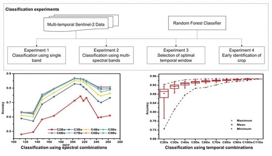
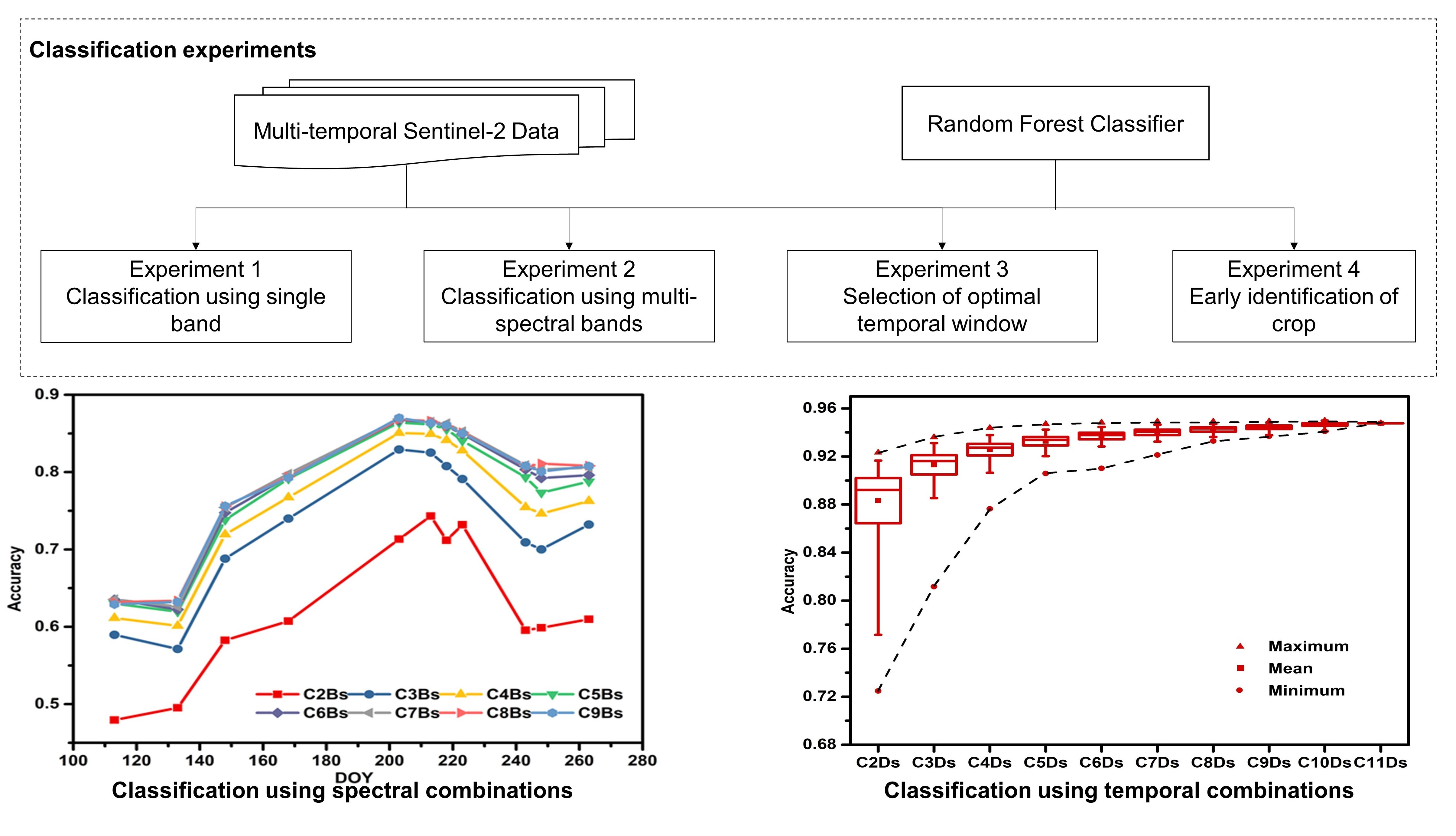
3.2. Experiment Design

To solve the issues raised in the introduction (i.e., explore the influence of the spectral and temporal information of Sentinel-2 on crop classification and the suitable feature selection strategies), four experiments in different scenarios were designed. Firstly, “single-band based classification” was carried out. Then, the more complex method was used to explore all multi-band combinations our of 9 bands of Sentinel-2. The formula for calculating the number of all possible combinations is:

$$P{C}_{all}={\sum }_{i=2}^m\frac{m!}{i!\left(m-i\right)!}$$

(2)

where $P{C}_{all}$ is the number of all possible combinations, $m$ is the number of total bands (i.e., 9 in our study) and $i$ is the number of combined bands out of 9 spectral bands of Sentinel-2 for classification. All combinations were grouped into sub-groups (8 groups in this study) according to the number of spectral bands used, e.g., Group-1 is all possible combinations from 2 bands, Group-2 is all possible combinations from 3 bands and so on. Similar scheme was used for image date combinations to determine optimal temporal window. Finally, a classification experiment was designed for early identification of crops, this is done by stepwise adding new images following the crop growth process. Detailed experiment design was given in the following sections.

3.2.1. Classification Using Single Band

The aims of the first experiment were to test the performance of crop classification when a single band of Sentinel-2 is applied with and without multi-temporal information and identify the most sensitive bands in RF model. Firstly, spectral information from single band of a single day (representing different stage of crop growth) was used in the RF model. To further identify the significance of temporal information, single band data of all 11 days were also applied. The difference of classification results by using different bands will be quantified by the inter-band comparison, and the accuracy with and without multi-temporal information will be evaluated.

3.2.2. Classification Using Multi-Spectral Bands

The second experiment is designed to explore how the band combinations influence the classification performance when applying them to the RF model. An enumeration method was applied to explore all possible combinations of 9 spectral bands, summing up to 502 combinations. Accuracy of classification results from the trained RF models by using all 502 band combinations from both single day images and multi-temporal images was evaluated. The 502 possible combinations, which were put into 8 groups according to the number of bands used for combination in each group, e.g., Group-1 was composed with 2 bands, Group-2 with 3 bands and Group 8 with 9 bands. The band combinations within each group resulted in different accuracy due to different abilities to identify vegetation properties. We then recorded the best combination in each group to find out which bands combinations performed best. According to the order and frequency of the bands appearing in the best combinations, we could summarize how the classification accuracy varies with the numbers and attributes of band combinations.

3.2.3. Selection of the Optimal Temporal Window

The third experiment is proposed for selecting the optimal temporal window for crop classification. All the 9 bands will be used in each temporal window. Enumeration method was applied to explore all possible combinations of the 11 acquisition dates, resulting in a total 2036 temporal combinations. The accuracy of the classification results by using each combination in the trained RF model is accessed by the testing data. The 2036 temporal combinations will be divided into 10 groups based on the number of images used in crop classification, e.g., Group-1 was composed with 2 image combinations, Group-2 with 3 images and Group 10 with 11 images. The performance difference within each group was due to the different phenological information provided by the images at different periods. By comparing the accuracy of different groups, the influence of image number on classification accuracy can be quantified. We then recorded the best combination in each group to find out which temporal combinations performed best. We can determine the optimal temporal window by analyzing the order and frequency of different image dates appearing in the best combinations.

3.2.4. Early Identification of Crops

The last experiment is to explore the earliest identification time during the crops growing season. Initiated with DOY 113 in our study, Sentinel-2 images of upcoming dates in the dataset were stepwise added to the RF model for classification. This procedure would be repeated until DOY 260, consistent with the actual crop growth courses. We will evaluate if the accuracy of crop classification can be escalated progressively with adding new images with time, and up to which date (i.e., which period of crop growth) the classification can reach acceptable accuracy. The variation of overall accuracy will be monitored to study the ability of early crop type identification.

4. Results

4.1. Crop Classification Accuracy Using Single Band

Figure 3 gives the classification accuracy using single band of Sentinel-2 on a single day. All results show eminently low accuracy (overall accuracy: 0.16–0.53). Accuracy of crop classification is significantly increased with overall accuracy varying from 0.875 to 0.915 when using the multi-temporal images (11 day images) (Figure 4). The NIR band outperforms other bands, followed by Green, Red and SWIR-1 bands. The surface reflectance of Green, Red and RE-1 bands is sensitive to the chlorophyll concentration and their temporal information can be used to identify the difference in growing stages among different crops [49,50]. The surface reflectance of SWIR-1 band is a good indicator for canopy water content which is also varied during the different growing stages and therefore significant for crop classification.

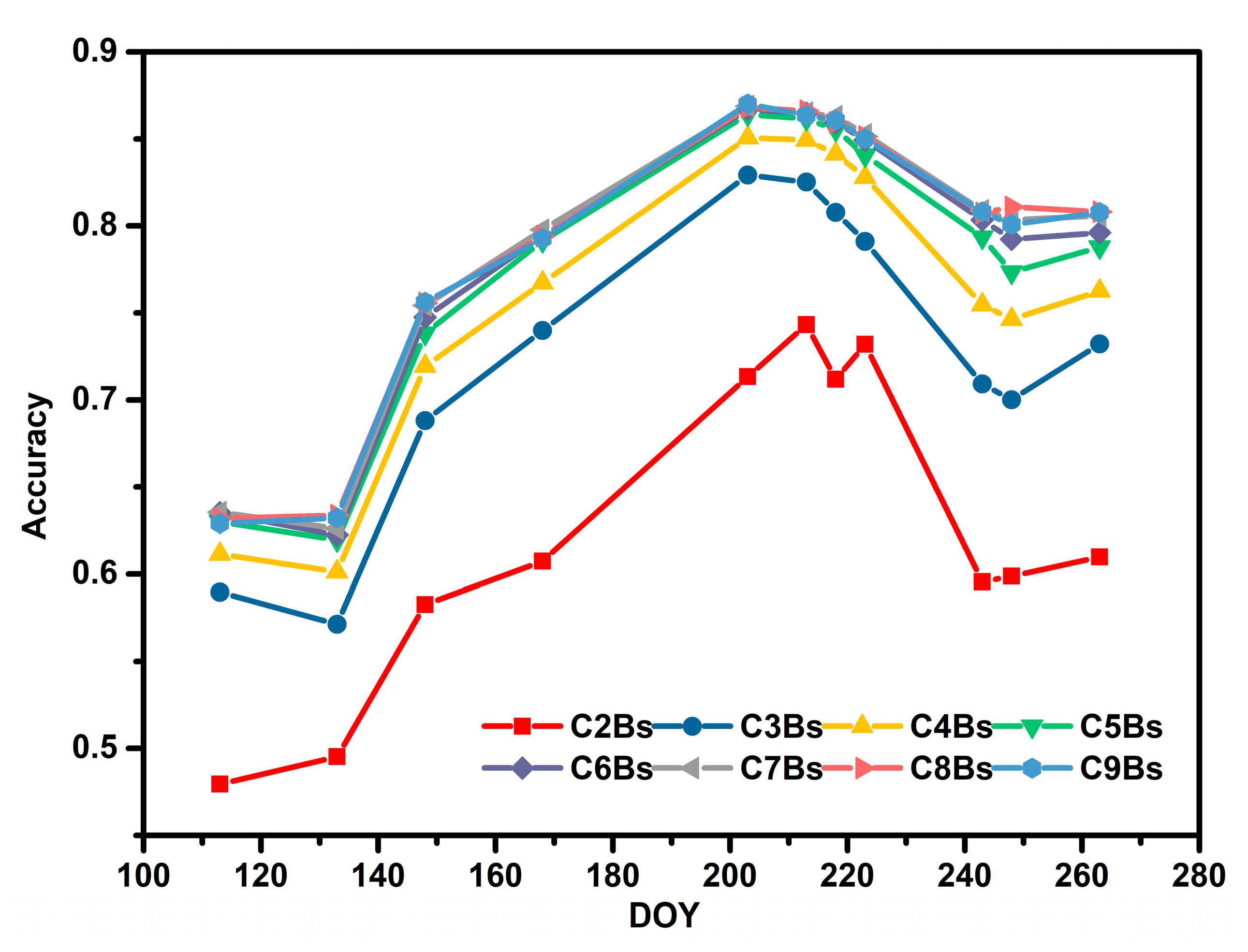
4.2. Crop Classification Accuracy Using Multi-Spectral Bands

4.2.1. Spectral Combinations on Single Date

Within normal cognition, multi-spectral combination provides more information and procures higher crop classification accuracy. In this section, we analyze how the multi-spectral information influenced the performance of crop classification in Shiyang River Basin. Firstly, multi-spectral combinations on a single date were tested (Figure 5). The term CxBs (Combined x Bands with x = 2, 3, 4, 5, 6, 7, 8 and 9) in Figure 5 refers to x number of bands combined in classification and only the best combination within each group was recorded. As shown in Figure 5, more Sentinel-2 spectral bands led to a higher classification accuracy. The most significant improvement attributed to the band number increasing from 2 to 3 and the accuracy was saturated when the number of bands reached 5. In addition, all the combinations in the growing season showed an analogous accuracy variation in time. The accuracy was low on DOY 113 and DOY 133, then increased from DOY 133 to DOY 203 with peak accuracy appeared around DOY 203, followed by a slight decrease between DOY 223 and DOY 263. For all the combinations, DOY 203-DOY 223 (mid of July, middle growing stage) was the crucial period for obtaining the highest classification accuracy.

Table 5. The combinations from 2 to 5 bands and corresponding periods that led to the best performance in crop classification in the Shiyang River Basin, 2019.

DOY	Spectral Bands and Overall Accuracy (OA) of Best Combinations
	C2Bs	OA	C3Bs	OA	C4Bs	OA	C5Bs	OA
203	B5, B11	0.71	B4, B5, B11	0.83	B4, B6, B11, B12	0.85	B4, B6, B8, B11, B12	0.86
213	B5, B11	0.74	B5, B11, B12	0.83	B4, B5, B8, B11	0.85	B4, B5, B8, B11, B12	0.86
218	B5, B11	0.71	B5, B6, B11	0.81	B5, B8, B11, B12	0.84	B2, B5, B8, B11, B12	0.85
223	B5, B11	0.73	B5, B6, B11	0.80	B5, B8, B11, B12	0.83	B4, B5, B8, B11, B12	0.84

showed the band combination pattern with the highest classification accuracy from C2Bs to C5Bs on DOY 203-DOY 223. The bands RE-1 and SWIR-1 almost occurred frequently in all the best combinations. We could infer that bands RE-1 and SWIR-1 play important roles throughout the middle growing season in multi-spectral crop classification. The result is consistent with that in Section 4.1, and the importance of Green and Red, which are also related to the chlorophyll concentration of crops, is weakened due to information redundancy.

4.2.2. Spectral Combinations with Multi-Temporal Information

The same spectral combinations of Sentinel-2 data from all the 11 days as in Section 4.2.1 in the Shiyang River Basin were applied to the RF model. Combinations were grouped into C2Bs to C9Bs by the number of spectral bands used in classification.

Table 6. Best combinations for different groups when using spectral combinations with full time series.

Combinations	Band of Sentinel-2	Overall Accuracy
C2Bs	RE-1, SWIR-1	0.94
C3Bs	RE-1, NIR, SWIR-1	0.95
C4Bs	GREEN, RE-1, NIR, SWIR-1	0.95
C5Bs	BLUE, Red, RE-1, NIR, SWIR-1	0.95
C6Bs	BLUE, GREEN, Red, RE-1, NIR, SWIR-1	0.95
C7Bs	All bands without Red and SWIR-2	0.95
C8Bs	All bands without Red	0.95
C9Bs	All bands	0.95

showed the maximum overall accuracy and the spectral bands used for classification in each group. With multi-temporal information, the overall accuracy increased to over 0.94 for all the spectral combinations and the highest overall accuracy was 0.95. The accuracy could be promoted by 8%–19% when applying temporal information with comparison to the results from using multi-spectral combinations on single date only. Although, the accuracy of crop classification increased when more bands of Sentinel-2 data were used, the addition of temporal information made this increment limited compared to the results of Section 4.2.1. The overall accuracy reached saturation when the number of bands reached 3. As the result shows, bands RE-1 and SWIR-1 appear in all the best combinations, which was similar to the results in spectral combinations on single date. The two-band combination, RE-1 and SWIR-1, could provide a satisfactory accuracy for crop classification. In summary, RE-1 and SWIR-1 were the most indispensable components for multi-spectral crop classification in the Shiyang River Basin. They respected the chlorophyll concentration and water content status of crops, respectively.

4.3. Selecting Optimal Temporal Window

Herein, we tried to find out the optimal temporal window for crop classification in the Shiyang River Basin. As described in Section 3.2.3, the 2036 combinations were grouped into 10 groups according to the number of dates used for classification. A boxplot graph is used to show the accuracy distributions with the maximum, upper quartile, median, mean, lower quartile and minimum values of the accuracy within each group (Figure 6). The term CxDs (Combined x images from different Dates with x = 2, 3, 4, 5, 6, 7, 8, 9, 10 and 11) in Figure 6 refers to x number of different dates images used in classification. Figure 6 illustrated that considering more dates lead to a higher classification accuracy. More importantly, as shown by the minimum and maximum accuracy in each group, the image acquisition time (period of growing stage) had a greater impact on the classification accuracy. When less number of dates used, the accuracy within each group varied more greatly.

Table 7. Best combinations for different groups of temporal combinations.

Combinations	DOY	Overall Accuracy
C2Ds	213, 243	0.92
C3Ds	148, 213, 248	0.94
C4Ds	148, 168, 213, 243	0.95
C5Ds	148, 168, 203, 213, 243	0.95
C6Ds	148, 168, 203, 213, 218, 248	0.95
C7Ds	133, 148, 168, 203, 213, 223, 248	0.95
C8Ds	133, 148, 168, 203, 213, 218, 223, 248	0.95
C9Ds	113, 148, 168, 203, 213, 218, 223, 248, 263	0.95
C10Ds	113, 148, 168, 203, 213, 218, 223, 243, 248, 263	0.95
C11Ds	113, 133, 148, 168, 203, 213, 218, 223, 243, 248, 263	0.95

displayed the image dates and overall accuracy of the best combinations for different groups of temporal combinations. The images from DOY 213 and DOY 248 (middle and late season) outperformed other combinations when only two images were used for classification, and DOY 213 and DOY 248 (or DOY 243) appeared in all the 10 best combinations. This indicated that middle (around DOY 213) and late periods (around DOY 248) were the crucial temporal windows for crop classification in the Shiyang River Basin. Just as important, there was still a gap between the best performance of the two (DOY 213 and DOY 248) image combinations (overall accuracy: 0.92) and the highest accuracy in the experiment (overall accuracy: 0.95). The satisfactory accuracy (overall accuracy: 0.95) could be achieved by considering four dates, and the maximum overall accuracy in C4Ds was got when DOY 148, 168, 213 and 248 were applied (Table 7). DOY 148 and 168 were in the early stages of the growing season in the Shiyang River Basin, crops emerged sequentially and grew rapidly. DOY 213 was in the middle stages of growing season of Shiyang River Basin when the coverage of most crops reached its peak. DOY 248 was in the late stages of growing season in the Shiyang River Basin when most crops were harvested sequentially. The use of data from three different periods (early, middle and late stages of the growing season) can comprehensively reflect the difference of crop growth period and its physical and chemical properties and therefore harvested the best classification performance.

4.4. Early Identification of Crop Types

Earlier crop identification might provide helpful information for agricultural management and decision-making. An experiment was developed to investigate how early in a year of growth we could complete crop mapping and obtain a satisfactory accuracy. In our case, DOY 113 was set as the starting date with the ending date changing from DOY 113 to DOY 263 successively. All data between the starting date and ending date were used to perform crop classification. This experiment was performed using all the 9 Sentinel-2 bands data in the RF algorithm. In Figure 7a, number n in the x-axis represented all data from DOY 113 to DOY n to train the model, the left y-axis refers to overall accuracy, and the right y-axis stands for accuracy change rate. The overall classification accuracy became higher with crop growing. The accuracy of crop classification increased significantly between DOY 110 and DOY 170, surpassed 0.9 at DOY 203, and became stable at a value around 0.95 on DOY 213 (middle stage of growth season in the Shiyang River Basin), which was also supported by the accuracy change rate approaching 0 on DOY 213 (Figure 7a). Associated with the crop phenology of the Shiyang River Basin, all crops except wheat and alfalfa were in the early stages of vegetative growth between DOY 110 and DOY 170. Predictably, various sowing dates and different vegetation canopy development patterns brought out evident spectral-temporal differences among the crops of the region. Figure 7b demonstrated the results of the F1 Score of each crop with the temporal development. The F1 score of wheat and alfalfa reached a peak at 0.99 on DOY 168 (mid-July) due to their unique phenological characteristics. During this period, alfalfa was harvested for the first time in current year, and wheat started its reproductive growth. The F1 Score of other crops between DOY 113 and DOY 168 showed a rapid increasing trend, consistent with the variation tendency of the overall classification accuracy. The F1 Score of corn, sunflower and melon2 reaches a stable value on DOY 203, fennel on DOY 213, interplant of sunflower and melon on DOY 223, and melon1 on DOY 243 (Figure 7b).

4.5. Basin-Scale Crop Classification Mapping

According to the analysis in Section 4.1, Section 4.2, Section 4.3 and Section 4.4, the band combination (RE-1, NIR and SWIR-1) on the four periods (DOY 148, DOY 168, DOY 213 and DOY 243) were considered as the optimal feature sets in the RF model for crop classification mapping in the Shiyang River Basin. The crop map based on this strategy was exhibited in Figure 8. The results of the confusion matrix were exhibited in

Table 8. Confusion matrix of the test samples by random forest (RF) classifier using 12 spectral-temporal features from Sentinel-2 data in the Shiyang River Basin in 2019.

Actual Types	Classified								Total	PA
	M1	FN	SF	SM	AL	M2	WH	CO
M1	115	2		1		2	1	19	140	0.82
FN	1	523	56	1				14	595	0.88
SF	19	13	979		1			16	1028	0.95
SM	1			354	5		7	11	378	0.94
AL		1	2		999	3	1	3	1009	0.99
M2			47	1		322	0	2	372	0.87
WH		4	1				658		663	0.99
CO	1	5	15	41	2	4		672	740	0.90
Total	137	548	1100	398	1007	331	667	737	4925
UA	0.84	0.95	0.89	0.89	0.99	0.97	0.99	0.91
OA = 0.94					Kappa = 0.93

, and classification resulted in the highest overall accuracy in our experiments (11 images with all spectral bands) were used as a reference (

Table 9. Confusion matrix of the test samples by RF classifier with highest accuracy from multi-temporal Sentinel-2 data (99 spectral-temporal features) in the Shiyang River Basin in 2019.

Actual Types	Classified								Total	PA
	M1	FN	SF	SM	AL	M2	WH	CO
M1	120					5		15	140	0.86
FN	0	561	20					14	595	0.94
SF	26	10	985					7	1028	0.96
SM				357	11		2	8	378	0.94
AL			2	1	999	2	0	5	1009	0.99
M2		1	51	0		320	0		372	0.86
WH		4					659		663	0.99
CO	1	1	12	49	1	2		674	740	0.91
Total	147	577	1070	407	1011	329	661	723	4925
UA	0.82	0.97	0.92	0.88	0.99	0.97	0.99	0.93
OA = 0.95					Kappa = 0.94

). The overall accuracy of the classification using the optimal feature combination (12 features) was 0.94, which was only 0.01 lower than the highest accuracy (by using total 99 features). It proved that our feature selection was reliable for crop classification in the Shiyang River Basin. As shown in the confusion matrix (Table 8), the producer and user accuracy of wheat and alfalfa both reached 99%, and the minimum user or producer accuracy of the remaining crops was also greater than 0.82. The phenomenon of mis-classified crops existed among crops with similar phenology. For instance, a small number of fennel and melon2 were mistakenly divided into sunflowers and some corns was wrongly divided into crops sunflower and the interplanted sunflower-melon.

5. Discussion

In this study, we conducted a series of experiments on crop classification in the Shiyang River Basin with multi-temporal Sentinel-2 data. The results of the experiments provide a fundamental basis to respond to the issues how the use of various information of Sentinel-2 data would influence the classification accuracy.

5.1. The Impact of Multi-Spectral Information on Crop Classification

The unique multi-spectral bands of Sentinel-2 have drawn much attention since the three red-edge bands of Sentinel-2 can provide abundant spectral information on vegetation monitoring. In our study, combining different bands increases the overall accuracy of crop classification. Red-edge band 1 (RE-1) and shortwave-infrared band 1 (SWIR-1) of Sentinel-2 were the most important component in the multi-spectral crop classification (Table 6 and Table 7). Previous studies reported that reflectance at SWIR bands was related to foliar water content [51,52], and had been used to estimate vegetation canopy water content and detect crop water stresses [51,52,53,54]. Meanwhile, Cai et al. [17] and Feng et al. [32] found that SWIR bands could distinguish soybean, corn and rice, due to the difference of canopy water contents between crops during the peak growing season. It is plausible that the difference of crop leaf water content is one of the key factors to identify crops. Another key factor may be the difference of crop chlorophyll. The study of Sun et al. [50] illustrated that RE-1 of Sentinel-2 was more significantly affected by the chlorophyll content of crop leaves compared with other bands. Meanwhile, many crops are in the transition stages between vegetative growth and reproductive growth with high foliar chlorophyll concentrations in the middle stages of growing season. Gitelson et al. [49] found that the green and red bands near 550 nm and 675 nm saturated at higher chlorophyll content, which limits the applications of green and red bands in crop classification somehow. Compared with the green and red bands, the higher sensitivity of chlorophyll concentration at the RE-1 provide essential information for crop classification.

5.2. The Impact of Temporal Information on Crop Classification

In terms of single-date classification, the overall classification accuracy was relatively low, especially when data from the early growing season were applied, reached the highest accuracy (accuracy > 0.8) from late July to early August, and then decreased at the end of the growing season (Figure 5). These findings were consistent with the conclusions in the study of Maponya et al. and Veloso et al. [26,55]. The low classification accuracy by data before June is attributed to the crops (sunflower, corn, melon, etc.) that have not yet grown in most areas in this period, which makes the sensor signals mix with a mass of soil background signals and interfere with the identification of target crops. With the growth of crops, changes in canopy structure and leaf pigment concentrations can offer more discernible information for RF to mine the differences among crops more effectively and increase the accuracy significantly. As crops start their reproductive growth, the unique properties of the crops gradually emerge and the classification accuracy reaches the maximum (overall accuracy = 0.87). For example, fennel turns bright yellow with its flowering, alfalfa blooms purple flowers and corn differentiates its unique reproductive organs. The declined accuracy in the late growing season may be ascribed to the sudden removal of biomass after crop harvest. With the crop being harvested gradually, the interference of soil noise on the crop signal is enhanced, which reduces the classification accuracy.

Temporal information reflecting the phenology from multi-temporal images greatly increase the accuracy of crop classification. This finding is consistent with Hao et al. and Vuolo, et al. [56,57]. It is found in their studies that the temporal information elevated the crop classification accuracy by 10–15% compared to spectral-based information. In the Shiyang River Basin, we find images from the early, mid and late stages of the growing seasons are indispensable for achieving optimal performance in crop classification (Table 7 and Figure 6). In previous studies, the optimal tempotral window did not go through the whole growing season [16,53]. The difference is mainly due to the phenological characteristics of crops in the Shiyang River Basin. The phenology of major crops (except for wheat and alfalfa) in the Shiyang River Basin is similar with sowing in late April and harvesting in early September. Therefore, a high degree of overlap of crop phenology results in the need for more temporal information to increase classification accuracy.

Earlier information in crops distributions and types is beneficial for timely crop yield prediction, food security evaluation and the fast actions taken by local governments [7,31,58]. Previous studies have demonstrated the relationship between timeliness and classification accuracy. They found that classification accuracy increased continuously with the additional use of images from early to middle growing season, and high accuracy could be realized in the middle season [33,58]. This was also the case in the Shiyang River Basin, where the overall accuracy arrived at 0.94 from late July to early August, and the early recognition time of different crops was further studied in our work (Figure 7). The early identification time of wheat and alfalfa was identified in very early stage (DOY 168) due to their distinct crop phenology—wheat was planted at the end of March and harvested in mid-July, and alfalfa was harvested three times a year. Corn, sunflower, melon2 and fennel were recognized from late July to early August, while the early identification time of the interplanted sunflower-melon and the melon1 were in later periods from mid-August to late August. Except for Melon1, other crops could be identified about at least one month before harvest. The sowing and harvesting time of melon1 were earlier than melon2, but the early identification time was contrast with the crop calendar. It was caused by the similar crop calendar between melon1 and corn. Similar crop calendars increased the difficulty of identifying melon1, which was proved by the low user accuracy and producer accuracy of melon1 in the confusion matrix results of crop classification with full-time series data. This work showed the substantial potential of Sentinel-2 data for accurate and in-season crop classification.

5.3. The Selection Strategy of Spectral-Temporal Features

Our study is in agreement with that by Immitzer et al. [33] that using all available cloud-free images during the growing season is practicable to harvest high accuracy. Using all available images is not suitable for large area mapping with huge costs of data storage space and computing time. In addition, previous studies have reported a common issue called Hughes phenomenon in remote sensing classification. It referred that the classification accuracy would reduce with the dimensionality of the data increased [29,30]. Given the high-dimensional characteristics of multi-temporal Sentinel-2 data, we also evaluated how much information is enough for the optimal results in different scenarios of crop classification. As previously discussed, images from the early, mid and late stages of the growing seasons are indispensable for achieving optimal performance in crop classification. If images were selected for classification according to critical crop phenological stages, we found that four images were the best balance between classification accuracy and the number of images. This result is in agreement with that of [13,34], where the classification accuracy did not improve continuously with the increase of images. Hao et al. [59] also evaluated the impact of image numbers on classification accuracy and discovered that more than five images did not influence notably on overall accuracy. In addition, if only a subset of Sentinel-2 spectral bands is used, a combination comprised of bands RE-1 and SWIR-1 outperforms other combinations. These strategies can help us choose pivotal spectral and temporal information. With this knowledge as a guide, our requirement on remote sensing data with complete spectral space and regular time series will be reduced, which is important for crop classification in large areas.

5.4. Limitations

It is worthy of noting that there are some limitations in this study. The first limitation is that we manually selected the cloud-free images, which is not practical for applications over large areas or mapping of long time series. Alternative solutions are to utilize automatic cloud-masking algorithms to select suitable images [60] or to use image compositing to reduce the effect of cloud [61]. The second limitation is that a transferable method using historical samples has not been studied in this study. Although, the selection strategy of multi-temporal features founded in this work can help us choose optimal temporal window and construct suitable spectral feature space, it is not an automatic solution for mapping crops given that we used specific image dates which were happened to have clear images. In other word, we also need to collect samples from mapping year to re-train RF for crop classification. Using regularly spaced time series data may improve the generalization performance of trained classifier with historical samples [62]. Future work is needed to develop methods to use time series data and effective features to extend the samples from one year to another. Some researchers also found that spatial autocorrelation would influence the accuracy of classification [63]. For example, if a test field is close to a training field, the accuracy is likely to be higher. Similar to previous studies, we took representative crop samples in the fields and divided the sample fields into training and validation groups to reduce the impact of spatial autocorrelation on classification accuracy. However, we did not explore how the classification accuracy was influenced by distance between training fields and validation fields on the classification results. This is worthy of systematic study in the future.

6. Conclusions

This study investigated the use of multi-spectral and multi-temporal Sentinel-2 images and random forest model for crop classification in the Shiyang River Basin. In total, 11 dates of cloud-free Sentinel-2 images spread over the crop growing season in 2019 were employed. Systematic experiments were carried out to study how various spectral and temporal information from Sentinel-2 affected crop classification. We found that the spectral and temporal information had significant impacts on the crop classification performance. Detailed conclusions are as follows:

(1)

Reasonable choice of spectral band combinations can effectively improve the crop classification accuracy. The RE-1 and SWIR-1 bands of Sentinel-2 are more efficient in identifying crops than other bands in the Shiyang River Basin.

(2)

In single-date crop classification, images from the middle growth periods are most pivotal for crop classification.

(3)

Images including the early, mid and late stages of the growing season are indispensable for achieving optimal performance in crop classification. In this study, four images from the key temporal window can get the best trade-off among the classification accuracy and number of images to be used.

(4)

Sentinel-2 data in combination with the RF method have the potential for the early detection of crops. In the Shiyang River Basin, the time of in-season classification could be advanced in late July (DOY210) with the overall accuracy reaching 0.9. Wheat could be identified accurately as early as in mid-June (one month before harvest). Alfalfa could be mapped as early as in mid-June (the first harvest). Sunflower, melon2, fennel and corn could be recognized as early as early August (one month before harvest).

References

1. Ozdogan, M. The spatial distribution of crop types from modis data: Temporal unmixing using independent component analysis. Remote Sens. Environ. 2010, 114, 1190–1204. [Google Scholar] [CrossRef]
2. Lobell, D.B.; Thau, D.; Seifert, C.; Engle, E.; Little, B. A scalable satellite-based crop yield mapper. Remote Sens. Environ. 2015, 164, 324–333. [Google Scholar] [CrossRef]
3. Song, X.-P.; Potapov, P.V.; Krylov, A.; King, L.; Di Bella, C.M.; Hudson, A.; Khan, A.; Adusei, B.; Stehman, S.V.; Hansen, M.C. National-scale soybean mapping and area estimation in the united states using medium resolution satellite imagery and field survey. Remote Sens. Environ. 2017, 190, 383–395. [Google Scholar] [CrossRef]
4. Sakamoto, T.; Gitelson, A.A.; Arkebauer, T.J. Near real-time prediction of u.S. Corn yields based on time-series modis data. Remote Sens. Environ. 2014, 147, 219–231. [Google Scholar] [CrossRef]
5. See, L.; Fritz, S.; You, L.; Ramankutty, N.; Herrero, M.; Justice, C.; Becker-Reshef, I.; Thornton, P.; Erb, K.; Gong, P.; et al. Improved global cropland data as an essential ingredient for food security. Glob. Food Secur. 2015, 4, 37–45. [Google Scholar] [CrossRef]
6. Wardlow, B.D.; Egbert, S.L. Large-area crop mapping using time-series modis 250 m ndvi data: An assessment for the u.S. Central great plains. Remote Sens. Environ. 2008, 112, 1096–1116. [Google Scholar] [CrossRef]
7. You, N.; Dong, J. Examining earliest identifiable timing of crops using all available sentinel 1/2 imagery and google earth engine. ISPRS J. Photogramm. Remote Sens. 2020, 161, 109–123. [Google Scholar] [CrossRef]
8. Duro, D.C.; Franklin, S.E.; Dubé, M.G. A comparison of pixel-based and object-based image analysis with selected machine learning algorithms for the classification of agricultural landscapes using spot-5 hrg imagery. Remote Sens. Environ. 2012, 118, 259–272. [Google Scholar] [CrossRef]
9. Van Niel, T.G.; McVicar, T.R. Determining temporal windows for crop discrimination with remote sensing: A case study in south-eastern australia. Comput. Electron. Agric. 2004, 45, 91–108. [Google Scholar] [CrossRef]
10. Wardlow, B.; Egbert, S.; Kastens, J. Analysis of time-series modis 250 m vegetation index data for crop classification in the u.S. Central great plains. Remote Sens. Environ. 2007, 108, 290–310. [Google Scholar] [CrossRef] [Green Version]
11. Zhong, L.; Gong, P.; Biging, G.S. Efficient corn and soybean mapping with temporal extendability: A multi-year experiment using landsat imagery. Remote Sens. Environ. 2014, 140, 1–13. [Google Scholar] [CrossRef]
12. Conese, C.; Maselli, F. Use of multitemporal information to improve classification performance of tm scenes in complex terrain. ISPRS J. Photogramm. Remote Sens. 1991, 46, 187–197. [Google Scholar] [CrossRef]
13. Peña, M.A.; Brenning, A. Assessing fruit-tree crop classification from landsat-8 time series for the maipo valley, chile. Remote Sens. Environ. 2015, 171, 234–244. [Google Scholar] [CrossRef]
14. Lobell, D.B.; Asner, G.P. Cropland distributions from temporal unmixing of modis data. Remote Sens. Environ. 2004, 93, 412–422. [Google Scholar] [CrossRef]
15. Massey, R.; Sankey, T.T.; Congalton, R.G.; Yadav, K.; Thenkabail, P.S.; Ozdogan, M.; Sánchez Meador, A.J. Modis phenology-derived, multi-year distribution of conterminous u.S. Crop types. Remote Sens. Environ. 2017, 198, 490–503. [Google Scholar] [CrossRef]
16. Wardlow, B.D.; Egbert, S.L. A comparison of modis 250-m evi and ndvi data for crop mapping: A case study for southwest kansas. Int. J. Remote. Sens. 2010, 31, 805–830. [Google Scholar] [CrossRef]
17. Cai, Y.; Guan, K.; Peng, J.; Wang, S.; Seifert, C.; Wardlow, B.; Li, Z. A high-performance and in-season classification system of field-level crop types using time-series landsat data and a machine learning approach. Remote Sens. Environ. 2018, 210, 35–47. [Google Scholar] [CrossRef]
18. Oliphant, A.J.; Thenkabail, P.S.; Teluguntla, P.; Xiong, J.; Gumma, M.K.; Congalton, R.G.; Yadav, K. Mapping cropland extent of southeast and northeast asia using multi-year time-series landsat 30-m data using a random forest classifier on the google earth engine cloud. Int. J. Appl. Earth Obs. Geoinf. 2019, 81, 110–124. [Google Scholar] [CrossRef]
19. Zhong, L.; Hu, L.; Zhou, H. Deep learning based multi-temporal crop classification. Remote Sens. Environ. 2019, 221, 430–443. [Google Scholar] [CrossRef]
20. Gilbertson, J.K.; Kemp, J.; van Niekerk, A. Effect of pan-sharpening multi-temporal landsat 8 imagery for crop type differentiation using different classification techniques. Comput. Electron. Agric. 2017, 134, 151–159. [Google Scholar] [CrossRef] [Green Version]
21. Wu, M.; Yang, C.; Song, X.; Hoffmann, W.C.; Huang, W.; Niu, Z.; Wang, C.; Li, W.; Yu, B. Monitoring cotton root rot by synthetic sentinel-2 ndvi time series using improved spatial and temporal data fusion. Sci. Rep. 2018, 8, 2016. [Google Scholar] [CrossRef] [PubMed] [Green Version]
22. Campos, T.; García, H.; Martínez, B.; Sánchez, R.; Gilabert, M.A. A copernicus sentinel-1 and sentinel-2 classification framework for the 2020+ european common agricultural policy: A case study in valència (spain). Agronomy 2019, 9, 556. [Google Scholar] [CrossRef] [Green Version]
23. Immitzer, M.; Vuolo, F.; Atzberger, C. First experience with sentinel-2 data for crop and tree species classifications in central europe. Remote Sens. 2016, 8, 166. [Google Scholar] [CrossRef]
24. Nasrallah, A.; Baghdadi, N.; Mhawej, M.; Faour, G.; Darwish, T.; Belhouchette, H.; Darwich, S. A novel approach for mapping wheat areas using high resolution sentinel-2 images. Sensors 2018, 18, 2089. [Google Scholar] [CrossRef] [Green Version]
25. Piedelobo, L.; Hernández-López, D.; Ballesteros, R.; Chakhar, A.; Del Pozo, S.; González-Aguilera, D.; Moreno, M.A. Scalable pixel-based crop classification combining sentinel-2 and landsat-8 data time series: Case study of the duero river basin. Agric. Syst. 2019, 171, 36–50. [Google Scholar] [CrossRef]
26. Veloso, A.; Mermoz, S.; Bouvet, A.; Le Toan, T.; Planells, M.; Dejoux, J.-F.; Ceschia, E. Understanding the temporal behavior of crops using sentinel-1 and sentinel-2-like data for agricultural applications. Remote Sens. Environ. 2017, 199, 415–426. [Google Scholar] [CrossRef]
27. Zhang, H.; Kang, J.; Xu, X.; Zhang, L. Accessing the temporal and spectral features in crop type mapping using multi-temporal sentinel-2 imagery: A case study of yi’an county, heilongjiang province, china. Comput. Electron. Agric. 2020, 176, 105618. [Google Scholar] [CrossRef]
28. Hu, Q.; Wu, W.-B.; Song, Q.; Lu, M.; Chen, D.; Yu, Q.-Y.; Tang, H.-J. How do temporal and spectral features matter in crop classification in heilongjiang province, china? J. Integr. Agric. 2017, 16, 324–336. [Google Scholar] [CrossRef]
29. Pal, M.; Mather, P.M. An assessment of the effectiveness of decision tree methods for land cover classification. Remote Sens. Environ. 2003, 86, 554–565. [Google Scholar] [CrossRef]
30. Pal, M.; Mather, P.M. Assessment of the effectiveness of support vector machines for hyperspectral data. Future Gener. Comp. Syst. 2004, 20, 1215–1225. [Google Scholar] [CrossRef]
31. Inglada, J.; Vincent, A.; Arias, M.; Marais-Sicre, C. Improved early crop type identification by joint use of high temporal resolution sar and optical image time series. Remote Sens. 2016, 8, 362. [Google Scholar] [CrossRef] [Green Version]
32. Feng, S.; Zhao, J.; Liu, T.; Zhang, H.; Zhang, Z.; Guo, X. Crop type identification and mapping using machine learning algorithms and sentinel-2 time series data. IEEE J. Sel. Top. Appl. Earth Obs. Remote Sens. 2019, 12, 3295–3306. [Google Scholar] [CrossRef]
33. Immitzer, M.; Neuwirth, M.; Böck, S.; Brenner, H.; Vuolo, F.; Atzberger, C. Optimal input features for tree species classification in central europe based on multi-temporal sentinel-2 data. Remote Sens. 2019, 11, 2599. [Google Scholar] [CrossRef] [Green Version]
34. Meng, S.Y.; Zhong, Y.F.; Luo, C.; Hu, X.; Wang, X.Y.; Huang, S.X. Optimal temporal window selection for winter wheat and rapeseed mapping with sentinel-2 images: A case study of zhongxiang in china. Remote Sens. 2020, 12, 226. [Google Scholar] [CrossRef] [Green Version]
35. Yuan, Q.; Shen, H.; Li, T.; Li, Z.; Li, S.; Jiang, Y.; Xu, H.; Tan, W.; Yang, Q.; Wang, J.; et al. Deep learning in environmental remote sensing: Achievements and challenges. Remote Sens. Environ. 2020, 241, 111716. [Google Scholar] [CrossRef]
36. Zhu, X.X.; Tuia, D.; Mou, L.; Xia, G.; Zhang, L.; Xu, F.; Fraundorfer, F. Deep learning in remote sensing: A comprehensive review and list of resources. IEEE Geosc. Remote Sens. Mag. 2017, 5, 8–36. [Google Scholar] [CrossRef] [Green Version]
37. Kussul, N.; Lavreniuk, M.; Skakun, S.; Shelestov, A. Deep learning classification of land cover and crop types using remote sensing data. IEEE Geosci. Remote Sens. Lett. 2017, 14, 778–782. [Google Scholar] [CrossRef]
38. Lyu, H.; Lu, H.; Mou, L.; Li, W.; Wright, J.; Li, X.; Li, X.; Zhu, X.; Wang, J.; Yu, L.; et al. Long-term annual mapping of four cities on different continents by applying a deep information learning method to landsat data. Remote Sens. 2018, 10, 471. [Google Scholar] [CrossRef] [Green Version]
39. Debats, S.R.; Luo, D.; Estes, L.D.; Fuchs, T.J.; Caylor, K.K. A generalized computer vision approach to mapping crop fields in heterogeneous agricultural landscapes. Remote Sens. Environ. 2016, 179, 210–221. [Google Scholar] [CrossRef] [Green Version]
40. Erinjery, J.J.; Singh, M.; Kent, R. Mapping and assessment of vegetation types in the tropical rainforests of the western ghats using multispectral sentinel-2 and sar sentinel-1 satellite imagery. Remote Sens. Environ. 2018, 216, 345–354. [Google Scholar] [CrossRef]
41. Immitzer, M.; Atzberger, C.; Koukal, T. Tree species classification with random forest using very high spatial resolution 8-band worldview-2 satellite data. Remote Sens. 2012, 4, 2661–2693. [Google Scholar] [CrossRef] [Green Version]
42. Löw, F.; Michel, U.; Dech, S.; Conrad, C. Impact of feature selection on the accuracy and spatial uncertainty of per-field crop classification using support vector machines. ISPRS J. Photogramm. Remote Sens. 2013, 85, 102–119. [Google Scholar] [CrossRef]
43. Inglada, J.; Arias, M.; Tardy, B.; Hagolle, O.; Valero, S.; Morin, D.; Dedieu, G.; Sepulcre, G.; Bontemps, S.; Defourny, P.; et al. Assessment of an operational system for crop type map production using high temporal and spatial resolution satellite optical imagery. Remote Sens. 2015, 7, 12356–12379. [Google Scholar] [CrossRef] [Green Version]
44. Belgiu, M.; Drăguţ, L. Random forest in remote sensing: A review of applications and future directions. ISPRS J. Photogramm. Remote Sens. 2016, 114, 24–31. [Google Scholar] [CrossRef]
45. Su, X.; Li, J.; Singh, V.P. Optimal allocation of agricultural water resources based on virtual water subdivision in shiyang river basin. Water Resour. Manag. 2014, 28, 2243–2257. [Google Scholar] [CrossRef]
46. Breiman, L. Random forests. Mach. Learn. 2001, 45, 5–32. [Google Scholar] [CrossRef] [Green Version]
47. Pedregosa, F.; Varoquaux, G.; Gramfort, A.; Michel, V.; Thirion, B.; Grisel, O.; Blondel, M.; Prettenhofer, P.; Weiss, R.; Dubourg, V.; et al. Scikit-learn: Machine learning in python. J. Mach. Learn. Res. 2011, 12, 2825–2830. [Google Scholar]
48. Pelletier, C.; Valero, S.; Inglada, J.; Champion, N.; Dedieu, G. Assessing the robustness of random forests to map land cover with high resolution satellite image time series over large areas. Remote Sens. Environ. 2016, 187, 156–168. [Google Scholar] [CrossRef]
49. Gitelson, A.A.; Kaufman, Y.J.; Merzlyak, M.N. Use of a green channel in remote sensing of global vegetation from eos-modis. Remote Sens. Environ. 1996, 58, 298. [Google Scholar] [CrossRef]
50. Sun, Y.H.; Qin, Q.M.; Ren, H.Z.; Zhang, T.Y.; Chen, S.S. Red-edge band vegetation indices for leaf area index estimation from sentinel-2/msi imagery. IEEE Trans. Geosci. Remote Sens. 2020, 58, 826–840. [Google Scholar] [CrossRef]
51. Tucker, C.J. Remote sensing of leaf water content in the near infrared. Remote Sens. Environ. 1980, 10, 23–32. [Google Scholar] [CrossRef]
52. Yilmaz, M.T.; Hunt, E.R.; Jackson, T.J. Remote sensing of vegetation water content from equivalent water thickness using satellite imagery. Remote Sens. Environ. 2008, 112, 2514–2522. [Google Scholar] [CrossRef]
53. Ghulam, A.; Li, Z.-L.; Qin, Q.; Yimit, H.; Wang, J. Estimating crop water stress with etm+ nir and swir data. Agric. Forest. Meteorol. 2008, 148, 1679–1695. [Google Scholar]
54. Xiao, X.; Boles, S.; Frolking, S.; Li, C.; Babu, J.Y.; Salas, W.; Moore, B. Mapping paddy rice agriculture in south and southeast asia using multi-temporal modis images. Remote Sens. Environ. 2006, 100, 95–113. [Google Scholar] [CrossRef]
55. Maponya, M.G.; van Niekerk, A.; Mashimbye, Z.E. Pre-harvest classification of crop types using a sentinel-2 time-series and machine learning. Comput. Electron. Agric. 2020, 169, 105164. [Google Scholar]
56. Hao, P.; Zhan, Y.; Wang, L.; Niu, Z.; Shakir, M. Feature selection of time series modis data for early crop classification using random forest: A case study in kansas, USA. Remote Sens. 2015, 7, 5347–5369. [Google Scholar] [CrossRef] [Green Version]
57. Vuolo, F.; Neuwirth, M.; Immitzer, M.; Atzberger, C.; Ng, W.-T. How much does multi-temporal sentinel-2 data improve crop type classification? Int. J. Appl. Earth Obs. Geoinf. 2018, 72, 122–130. [Google Scholar]
58. Defourny, P.; Bontemps, S.; Bellemans, N.; Cara, C.; Dedieu, G.; Guzzonato, E.; Hagolle, O.; Inglada, J.; Nicola, L.; Rabaute, T.; et al. Near real-time agriculture monitoring at national scale at parcel resolution: Performance assessment of the sen2-agri automated system in various cropping systems around the world. Remote Sens. Environ. 2019, 221, 551–568. [Google Scholar] [CrossRef]
59. Hao, P.; Wu, M.; Niu, Z.; Wang, L.; Zhan, Y. Estimation of different data compositions for early-season crop type classification. Peerj 2018, 6, e4834. [Google Scholar]
60. Bai, T.; Li, D.; Sun, K.; Chen, Y.; Li, W. Cloud detection for high-resolution satellite imagery using machine learning and multi-feature fusion. Remote Sens. 2016, 8, 715. [Google Scholar]
61. Lück, W.; van Niekerk, A. Evaluation of a rule-based compositing technique for landsat-5 tm and landsat-7 etm+ images. Int. J. Appl. Earth Obs. Geoinf. 2016, 47, 1–14. [Google Scholar] [CrossRef]
62. Brinkhoff, J.; Vardanega, J.; Robson, A.J. Land cover classification of nine perennial crops using sentinel-1 and -2 data. Remote Sens. 2019, 12, 96. [Google Scholar] [CrossRef] [Green Version]
63. Stehman, S.V.; Foody, G.M. Key issues in rigorous accuracy assessment of land cover products. Remote Sens. Environ. 2019, 231, 111199. [Google Scholar]
Figure 1. Study area and locations of ground truth samples. The Shiyang River Basin is located in northwest China. The background image is mosaicked by 11 Sentinel-2 images on 1 August of 2019, projected in WGS84, in true color image (R = Band 4, G = Band 3 and B = Band 2).
Remotesensing 12 04052 g001
Figure 2. The workflow of crop classification by random forest method using Sentinel-2 multi-spectral images.
Remotesensing 12 04052 g002
Figure 3. Overall accuracy of crop classification using single band of Sentinel-2 on a single date in the Shiyang River Basin, 2019.
Remotesensing 12 04052 g003
Figure 4. Overall accuracy of crop classification using single band of Sentinel-2 and the multi-temporal information in the Shiyang River Basin, 2019.
Remotesensing 12 04052 g004
Figure 5. The best classification performance using different numbers of spectral bands on a specific date. The term CxBs (Combined x Bands with x = 2, 3, 4, 5, 6, 7, 8 and 9) refers to x number of bands combined for crop classification.
Remotesensing 12 04052 g005
Figure 6. Overall accuracy distributions of all 2036 temporal combinations. The term CxDs means x images of different acquisition dates that are combined for classification experiments.
Remotesensing 12 04052 g006
Figure 7. Changes in overall accuracy (a) and F1 Score (b) of crops as a function of date. For example, the DOY 203 in the x-axis means that all spectral bands from DOY 113 to DOY 203 were used to train RF and predicted class labels cooperating with training and testing samples. The blue line in (a) means overall accuracy of crops and red line refers to rate of accuracy change.
Remotesensing 12 04052 g007
Figure 8. Crop map derived from Sentinel-2 data with 10 m resolution in Shiyang River Basin, 2019.
Remotesensing 12 04052 g008