Snow and Ice Thickness Retrievals Using GNSS-R: Preliminary Results of the MOSAiC Experiment

Abstract

The FSSCat mission was the 2017 ESA Sentinel Small Satellite (S⌃3) Challenge winner and the Copernicus Masters competition overall winner. It was successfully launched on 3 September 2020 onboard the VEGA SSMS PoC (VV16). FSSCat aims to provide coarse and downscaled soil moisture data and over polar regions, sea ice cover, and coarse resolution ice thickness using a combined L-band microwave radiometer and GNSS-Reflectometry payload. As part of the calibration and validation activities of FSSCat, a GNSS-R instrument was deployed as part of the MOSAiC polar expedition. The Multidisciplinary drifting Observatory for the Study of Arctic Climate expedition was an international one-year-long field experiment led by the Alfred Wegener Institute to study the climate system and the impact of climate change in the Arctic Ocean. This paper presents the first results of the PYCARO-2 instrument, focused on the GNSS-R techniques used to measure snow and ice thickness of an ice floe. The Interference Pattern produced by the combination of the GNSS direct and reflected signals over the sea-ice has been modeled using a four-layer model. The different thicknesses of the substrate layers (i.e., snow and ice) are linked to the position of the fringes of the interference pattern. Data collected by MOSAiC GNSS-R instrument between December 2019 and January 2020 for different GNSS constellations and frequencies are presented and analyzed, showing that under general conditions, sea ice and snow thickness can be retrieved using multiangular and multifrequency data.

1. Introduction

FSSCat was the winner of the “2017 ESA Sentinel Small Satellite (S⌃3) Challenge” and the overall winner of the 2017 “Copernicus Masters” competition [1]. The mission consists of two “federated” 6U (10 × 20 × 30 cm³) CubeSats (³Cat5/A and ³Cat-5/B) in support of the Copernicus Land and Marine Environment services [2], which were successfully launched on 3 September 2020 onboard the Vega SSMS (Small Spacecraft Mission Service) maiden flight in a Sun Synchronous Orbit of 550 km height. The goal of the ESA S⌃3 Challenge was to develop, in a record time of one year, a novel small satellite mission to complement the Sentinel family missions. One of the instruments onboard FSSCat is the Flexible Microwave Payload-2 (FMPL-2) [3], a dual Global Navigation Satellite System reflectometer (GNSS-R) and microwave radiometer instrument implemented using a Software Defined Radio.

The GNSS signals produce a coherent reflection over the ice [4] that allows for the precise determination of the ice edge [5]. Moreover, other studies show the potential of GNSS-R measurements to infer sea-ice thickness, when the scattering is coherent and the complex reflected signals are downloaded to ground [6,7], based on the reflection between the sea-ice and the sea water underneath. However, this hypothesis has not been confirmed by in-situ measurements, as sea-ice thickness has been only retrieved at L-band by radiometers [8,9].

As part of the validation of the FMPL-2 GNSS-R instrument, the PYCARO-2 (P(Y) & C/A ReflectOmeter-2), an evolved version of PYCARO, [10] was designed to take part in the Multidisciplinary drifting Observatory for the Study of Arctic Climate (MOSAiC) expedition [11,12], the largest campaign ever aiming to study the Arctic Ocean.

The objective of MOSAiC was to understand the evolving Arctic climate system and the role it plays in changing the global climate. MOSAiC was a multidisciplinary campaign to study the Arctic Ocean from different points of view, and involving different teams: Ice, Ocean, Atmosphere, Ecology, Bio-geochemical systems, Satellite Remote Sensing, Modeling, and Aircraft teams. Most of them deployed a large suite of sensors to measure different parameters, such as ice thickness evolution, snow properties, the topography beneath the ice floe, etc. Most of the instruments run for over a year on top of a drifting ice floe. The diversity of simultaneous measurements and the extension of the campaign in time makes it an exceptional opportunity to cross-check and use the data retrieved as model validation for other sensors such as scatterometers, GNSS-R, or radiometer sensors on satellites. Here, we will focus on the MOSAiC remote sensing site and its ancillary measurements, which include:

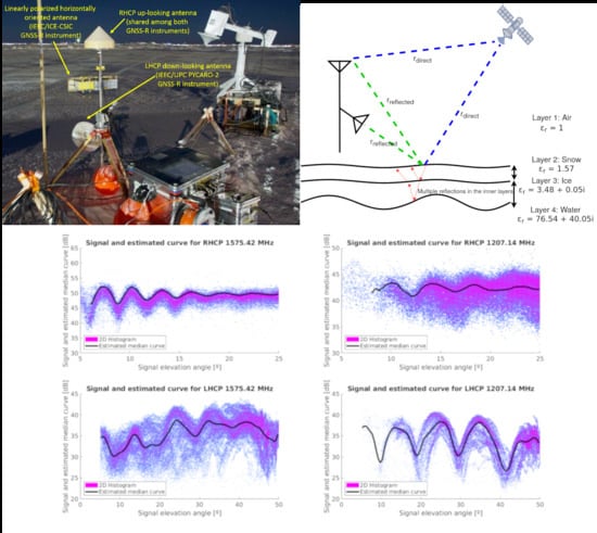
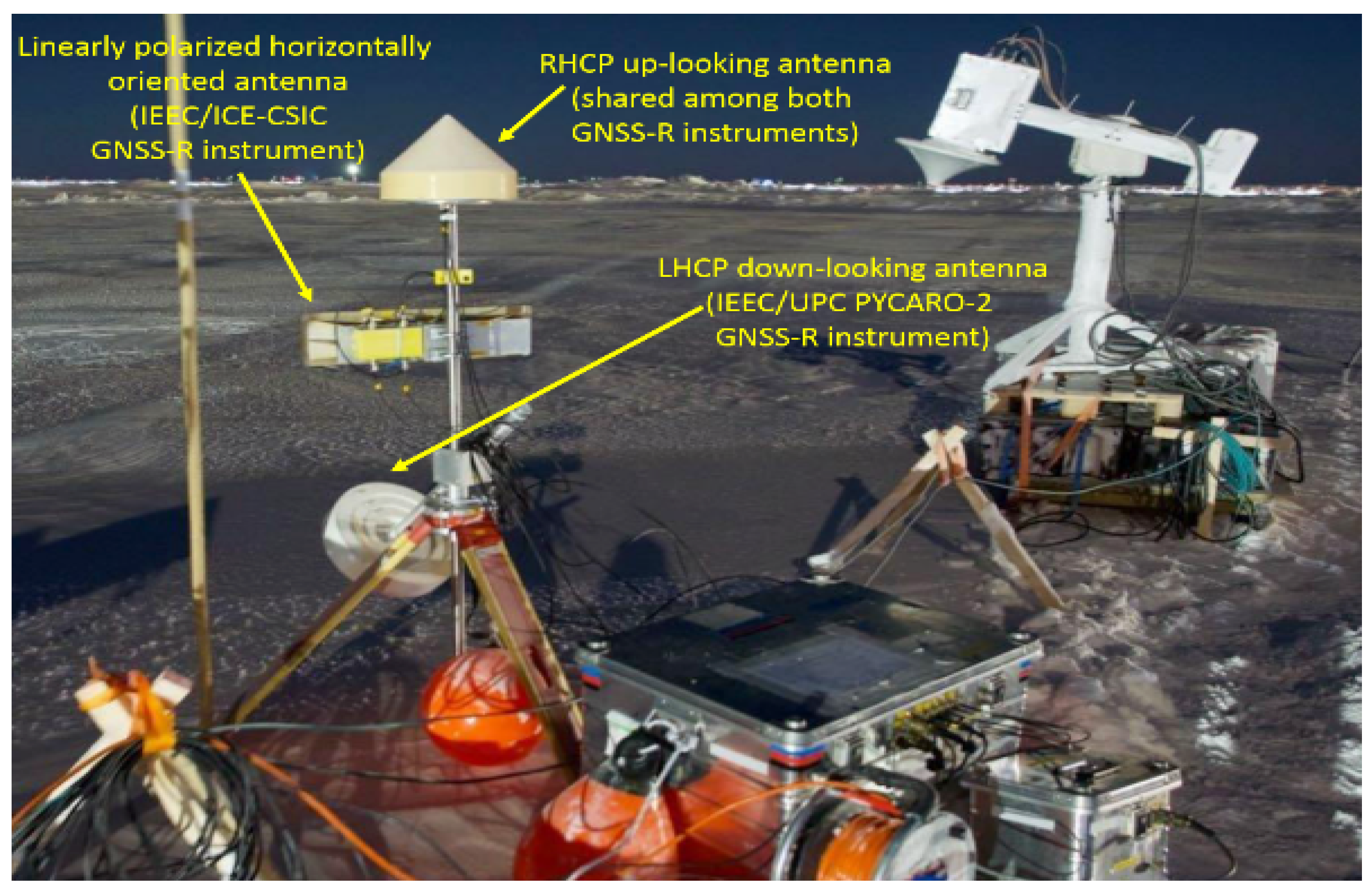
• Three Remote Sensing Sites (alternating measurements every 2–3 weeks), with the following instruments: L-, C-, X-, Ka-, and Ku-band microwave scatterometers, P- to L-band, C-, X-, Ku-, K-, and W-band microwave radiometers, IR and hyperspectral cameras, and two multiconstellation and multiband GNSS-R instruments. The GNSS-R instruments (Figure 1) are part of a joint effort from the Institut d’Estudis Espacials de Catalunya (IEEC): Institute of Space Sciences (ICE, CSIC), and Universitat Politècnica de Catalunya (UPC) IEEC sections.
• Regular transects (1 km length over different sea-ice types) to measure total sea ice thickness, snow depth and density, Ku- and Ka-band radar backscatter, L-band radiometry, and additionally surface albedo with the returning insolation from spring onwards.
• Other ice, snow, ocean, and atmospheric measurements.

This work describes the data collected by one of the GNSS-R instruments developed by IEEC/UPC. Section 2 describes the instrument, the experiment set up, and the ground truth data used, Section 3 describes the Interference Pattern captured by the instrument, produced by the sea-ice floe, modeled as a four-layer dielectric, and Section 4 analyzes the results of the data retrieved by the PYCARO-2 IEEC/UPC instrument and its comparison to the four-layer model is presented in Section 3.

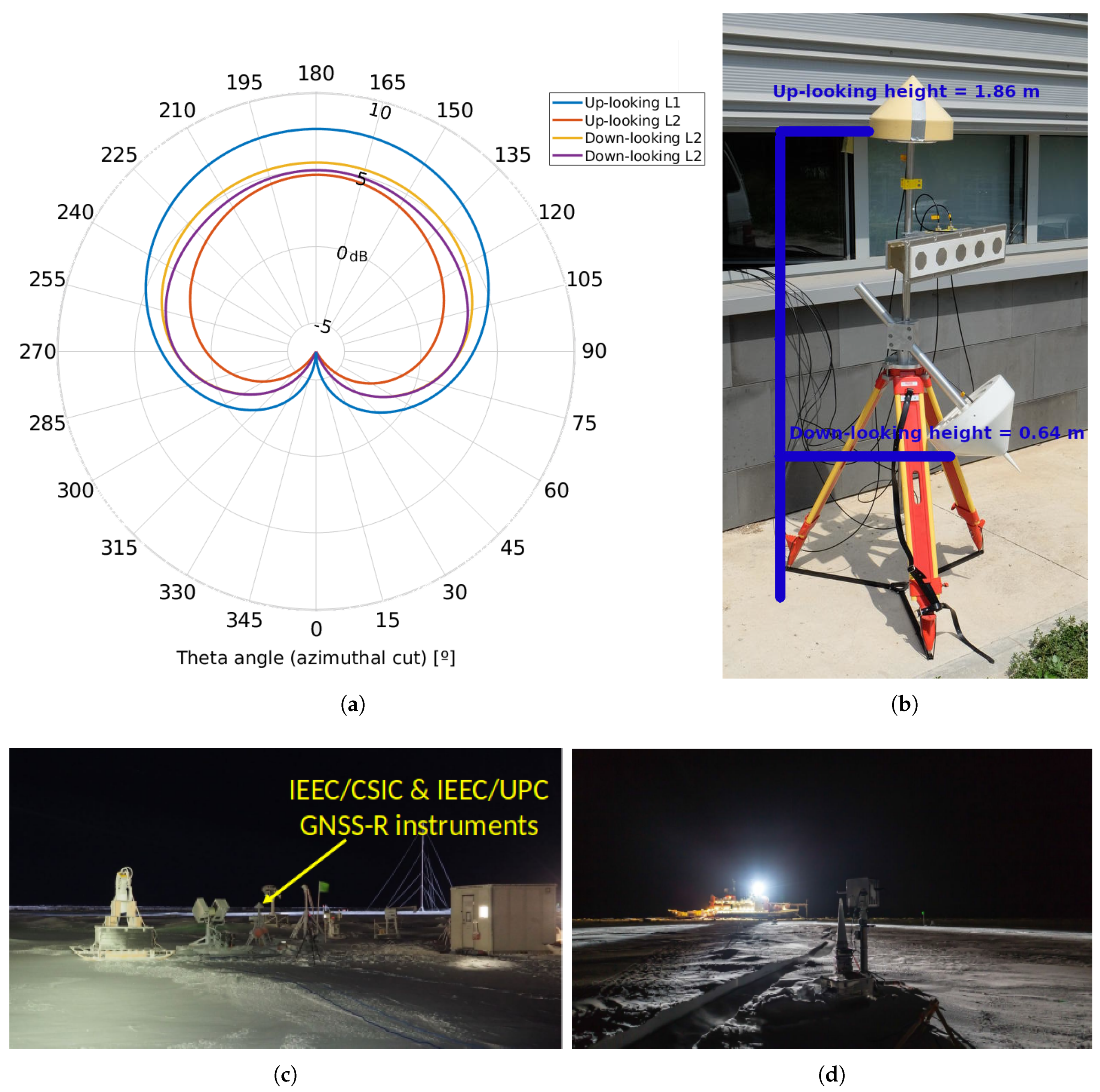
2. Instrument Description and Experiment Setup

The GNSS-R instruments belonging to the Remote Sensing site are divided in two. One of them is the ICE/CSIC instrument, which is a GNSS-R instrument working at linear polarization to collect the reflected signals off the sea-ice. Its aim is to provide sea-ice properties from scattered GNSS signals. The other one is the IEEC/UPC instrument (named PYCARO-2), which operates at Left hand Circular Polarization (LHCP) and aims to support the reflectivity modeling activities in support to the FMPL-2 data processing.

Both instruments share a common power and data interface, physical enclosure, and the Right Hand Circular Polarization (RHCP) antenna used for time and geo-reference the instrument. The primary objective of both GNSS-R instruments is to provide ground-truth data for reflection modeling and originally also to support the calibration/validation of the FMPL-2 [3] onboard the FSSCat mission [1,2]. This manuscript focuses only on the data retrieved by the IEEC/UPC PYCARO-2 instrument [13], which is equipped with an antenna working at the same polarization (LHCP) as the FMPL-2 instrument onboard FSSCat.

2.1. Circular Polarization GNSS-R Instrument

PYCARO-2 is an evolved version of the PYCARO instrument, which was the first GNSS-R instrument collecting polarimetric reflected Galileo signals from a stratospheric balloon (Bexus 19 in 2014 [14]). PYCARO was also the payload of the UPC ³Cat-2 CubeSat [15]. PYCARO-2 is able to track Beidou B1/B2 in addition to GPS L1/L2 and Galileo E1/E5, as well as GLONASS L1/L2.

The down-looking antenna is a LHCP choke-ring antenna, tilted 45° downwards to maximize the power of the reflected signals, as most GNSS satellites reach ∼50° elevation angle in polar regions. The antennas have a very smooth radiation pattern, as shown in Figure 2a and their configuration (height and pointing) can be seen in Figure 2b.

The instruments were shipped to Tromsø, Norway, on July 2019, from where the Polastern icebreaker carrying the MOSAiC expedition departed on 20 September 2019. The Remote Sensing (RS) site was set up during October 2019, and the instruments were successfully installed on 24 October 2019, as shown in Figure 2c. Despite being installed in October, several ice cracks (Figure 2d) during November and December forced a relocation of the RS site, including the PYCARO-2 instrument. The final location of the instrument for the winter season was set in late December 2019.

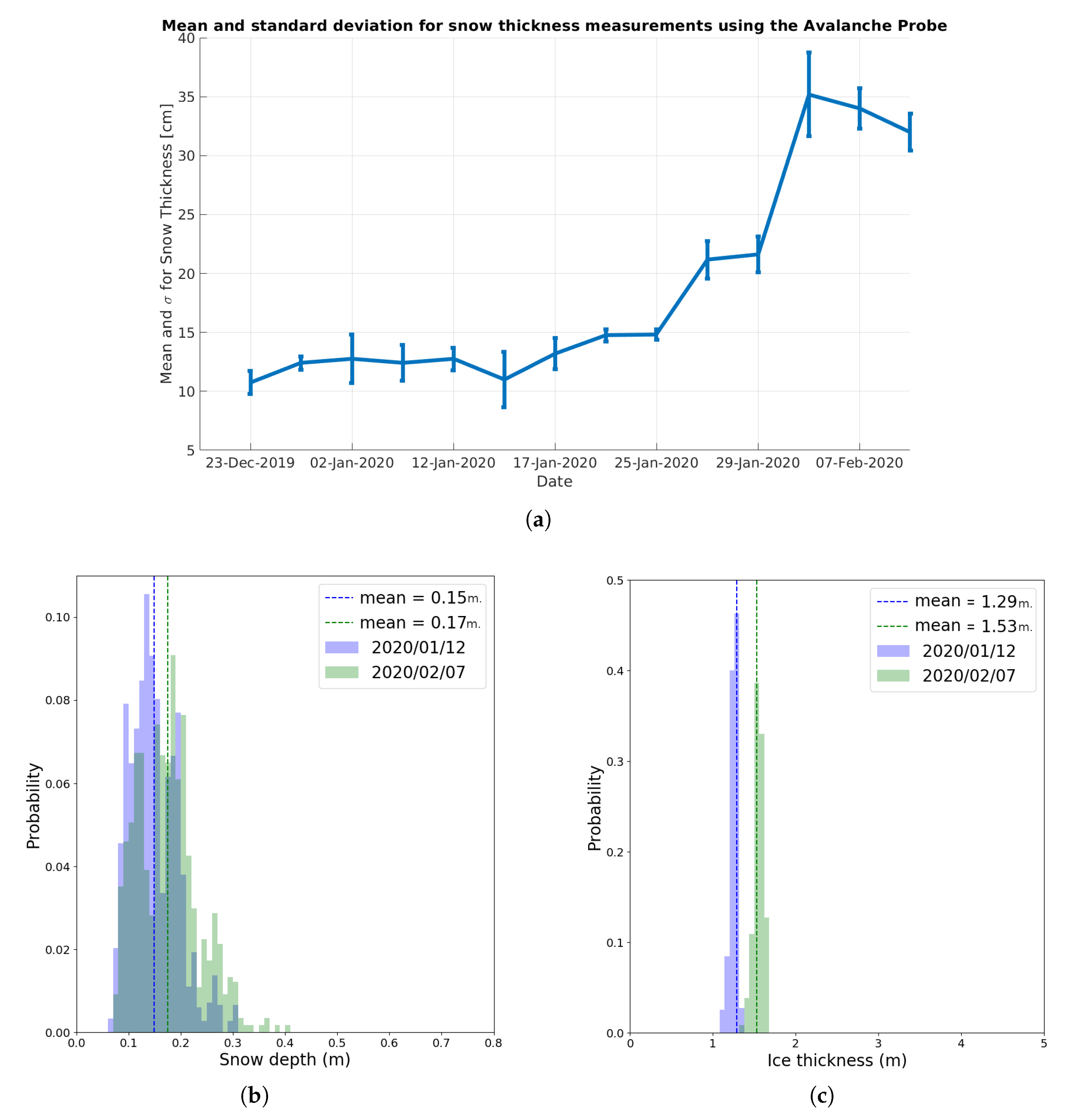
2.2. Ground-Truth Data

In the vicinity of the GNSS instrument, different types of measurements were collected of both snow depth, and sea ice thickness. Measurements were repeated every few weeks by the combination of a Magnaprobe snow probe and broadband electromagnetic induction sensors (Geophex GEM-2). The Magnaprobe was used to retrieve snow thickness, with a precision better than 1 cm [16]. The GEM-2 was used to measure the combined thickness of the snow and the sea ice, as described by [17]. Finally, both measurements are combined to retrieve snow and sea-ice thickness separately. In this study, we use the quick-view GEM-2 thicknesses based on the 18 kHz in-phase channel and processed directly onboard and quality controlled against manual drill-hole observations. We chose this channel out of the available frequency set of the GEM-2 for optimal retrieval of sea ice thickness with an accuracy better than 10 cm.

The snow depth was also measured using an avalanche probe in the area surrounding the GNSS-R instrument mast. Figure 3a shows the evolution of the mean and standard deviation of the snow thickness in the area surrounding the GNSS instrument. Figure 3b shows a broad distribution of snow depths as a Probability Distribution Function (PDF) and points to a highly inhomogeneous snow surface, with developed snow dunes in two different time instants (blue, 12 January 2020, and green, 7 February 2020). Finally, Figure 3c shows the PDF of the sea-ice thickness measurements.

It can be observed that, for the period between December 2019 and January 2020, the PDF and the avalanche probe measurements are consistent, which is not the case for February 2020. The instrument performance is compared to these measurements, from where consistent ground-truth data is available. Furthermore, ice core drillings were performed during the first days of December, showing that the ice core during the week of the 21st of December 2019, was around 0.8 m and 1 m thick. The same ice core drillings were conducted in the time period shown in Figure 3c to validate the measurements taken by the Magnaprobe.

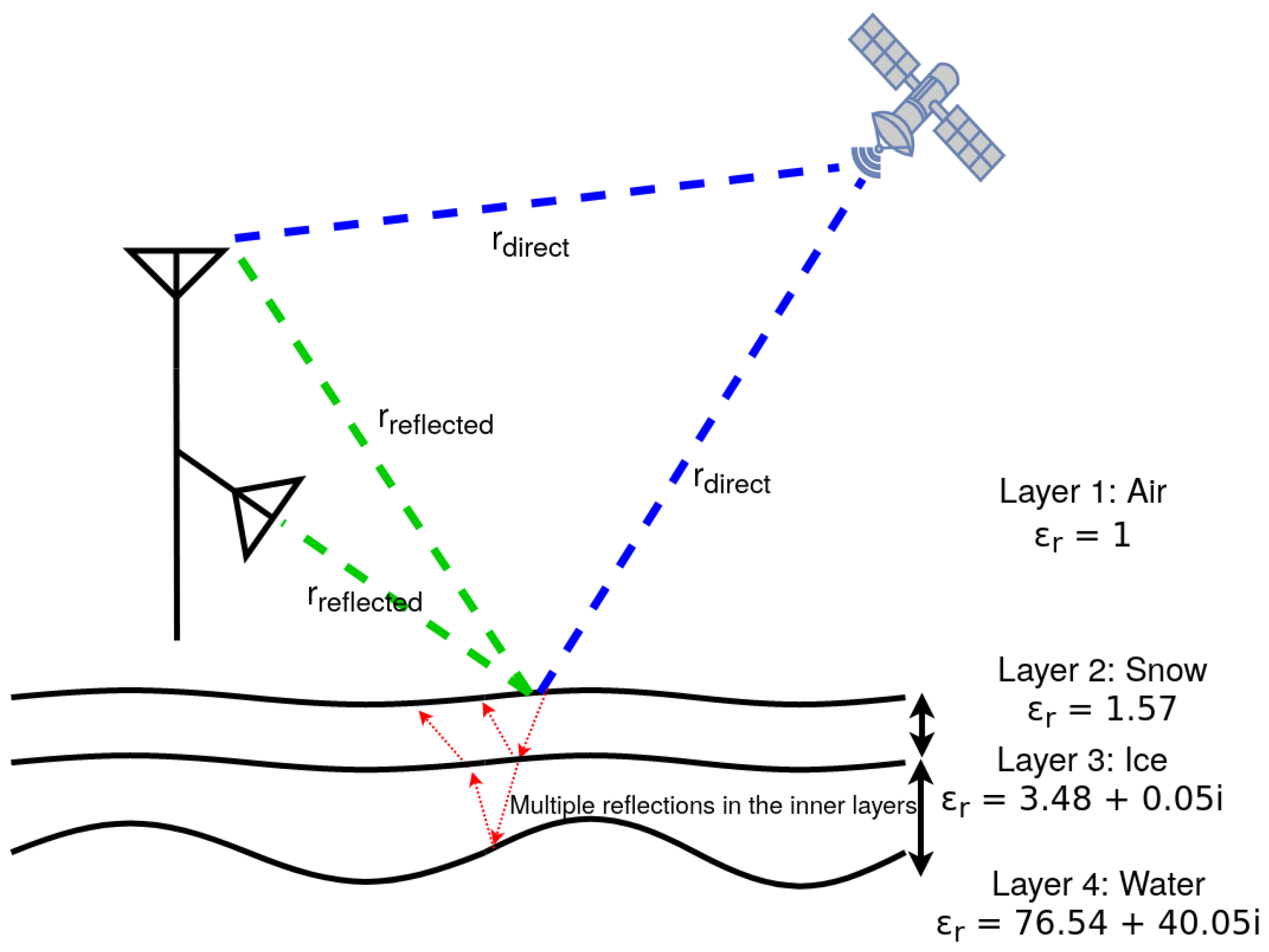
3. Theoretical Background: IPT Applied to the Ice Floe

In navigation receivers, multipath is avoided as much as possible as it degrades positioning accuracy. For ground-based GNSS-R instruments, the signal collected by a GNSS antenna is a combination of the incident wave, i.e., the one coming directly from the GNSS satellite at RHCP and the signal reflected over a certain surface. The combination of the direct and reflected signals creates strong reflectivity fluctuations or fringes, called an “Interference Pattern”. In the PYCARO-2 case, the reflection of the GNSS signal on the sea ice floe produced the same type of fluctuations.

The Interference Pattern Technique (IPT) was conceived by [18] to extract a number of geophysical parameters from the Earth by means of ground-based instruments. Most of its applications are soil moisture [19], vegetation height [20], water level [21] monitoring, sea state [22], or snow depth [23] estimation. However, most of those works are based on a three-layer model, with the first layer being air, a second thin layer of substrate (i.e., snow, crop field), and finally, a third layer which is a semi-infinite reflective surface (i.e., land). Interfering reflections from multiple layers of snow and ice in Antarctica were analyzed in [24], however, according to the authors’ knowledge, the IPT has never been applied over an ice floe, which contains four dielectric layers: air, a snow layer on top of the sea ice, the sea ice itself, and the sea water underneath.

To study the Interference Pattern (IP) fringes created by the multiple reflections in the floe, the instrument retrieves the signal-to-noise ratio (or peak of the Delay-Doppler Map minus noise background measured a few lags before the correlation peak [25]) once every 10 s, collecting thousands of reflections from different bands and constellations. The total amount of reflections collected was 300.000 for Beidou B1D1, 125.000 for Beidou B2D1, 425.000 for Galileo E1C, 290.000 for Galileo E5b, 275.000 for GPS L1 C/A, and 235.000 for GPS L2 P(Y). The data used to perform this study was collected from 20 December 2019 to 27 January 2020. However, due to several operational procedures of the instrument, most of the data was obtained between 15 and 27 January 2020. This study is focused on the analysis of this period of data, from which results and methodology will then be applied to the rest of the campaign.

3.1. Four-Layer IPT Model: Theoretical Definition

The scattering geometry is modeled as shown in Figure 4, where the dielectric constant of each media as in Section 6.2 of [26], and in particular, the sea-ice dielectric constant model is based in [27], but for the direct model. This study is performed assuming the dielectric constant of the substrate is not varying. Furthermore, simulations have been performed to prove that the effect of varying the dielectric constant of the substrate produced a negligible effected as compared to the variation of either the snow or the ice thickness. In addition, the properties selected (i.e., snow density, ice type, and ice temperature) used to compute the dielectric constants shown in Figure 4 are the average values of what MOSAiC researchers’ measured. Therefore, following the procedures described in [28], the power received by either the zenith-looking or the 45°-looking antenna is proportional to (see Figure 2a).

$$P\left(\theta \right)\propto {\left|E_i\left({\theta }_i\right)+E_r\left({\theta }_i\right)\right|}^2={\left|E_0\right|}^2·{\left|F_n\left({\theta }_{dir}\right)+F_n\left({\theta }_{ref}\right)·R({ϵ}_r,{\theta }_i)·e^{j\Delta \varphi }\right|}^2,$$

(1)

where $E_i$ is the incident electric field, $E_r$ is the reflected electric field, $F_n\left(\theta \right)$ is the antenna voltage pattern (amplitude and phase) for the up-looking and down-looking signals arriving to either the up-looking or down-looking antennas, with different patterns for each one (see Figure 2a), ${\theta }_{dir}$, and ${\theta }_{ref}$ are the off-boresight arriving angles of the direct and reflected signals, ${\theta }_i$ is the incidence angle of the signal arriving from a particular GNSS spacecraft, $E_{0_i}$ is the direct signal, the one that would be received if there were no interference, $R({ϵ}_r,\theta )$ is the reflection coefficient as defined in (3), and $\Delta \varphi$ is the phase associated to the geometry. $\Delta \varphi$ is given by

$$\Delta \varphi =\frac{4\pi }{\lambda }·h·sin\left(\theta \right),$$

(2)

where $\lambda$ is the electromagnetic wavelength, depending on the frequency band (L1 or L2), h is the antenna height, and $\theta$ is the satellite elevation angle. The reflectivity on top of the snow layer is computed iteratively as

$$R_i=e^{-{\left(\frac{4\pi \sigma }{\lambda }\right)}^2}\frac{r_{i,i+1}+r_{i+1,i+2}·e^S·e^{j2\Psi }}{1+r_{i+1,i+2}·r_{i+1,i+2}·e^S·e^{j2\Psi }},$$

(3)

where $r_{i,i+1}$ is the Fresnel coefficients between layers i and i+1, for the four-layer model being 1 = air, 2 = snow, 3 = ice, and 4 = saline water; S (see (4)) accounts for the reflectivity decrease due to the roughness at the interface [18], and $\Psi$ is the phase produced by the reflection between the different layers, as detailed in (5)

$$S=-8·{\left(\frac{\pi \sigma }{\lambda }\sqrt{{\epsilon }_{r_{i+1}}-{\epsilon }_{r_i}·{cos}^2\left(\theta \right)}\right)}^2$$

(4)

$$\Psi =\frac{2\pi }{\lambda }{t}_{i+1}·\sqrt{{\epsilon }_{r_{i+1}}-{\epsilon }_{r_i}·{cos}^2\left(\theta \right)}$$

(5)

where $t_{i+1}$ is the thickness of the $i+1$ layer, ${ϵ}_{r_i}$ is the permittivity of the i layer, and $\sigma$ the surface roughness of the interface.

3.2. Four-Layer IP Model: PYCARO-2 Case

Each of the different surface permittivity values (${ϵ}_{r_i}$) for this study have been modeled. The snow has been modeled as dry snow, as per in-situ measurements during the expedition, with a density of 296 kg/m³, and −25 °C [29]. The ice has been modeled as multiyear ice, with a mean temperature of −25 °C. Note that simulations have been carried out at different temperatures, and the impact of varying the mean temperature is negligible in front of the interference pattern produced by variations on the layer thickness. Finally, the water layer has been modeled as saline water (32 psu) and at a temperature of −1.7 °C [29].

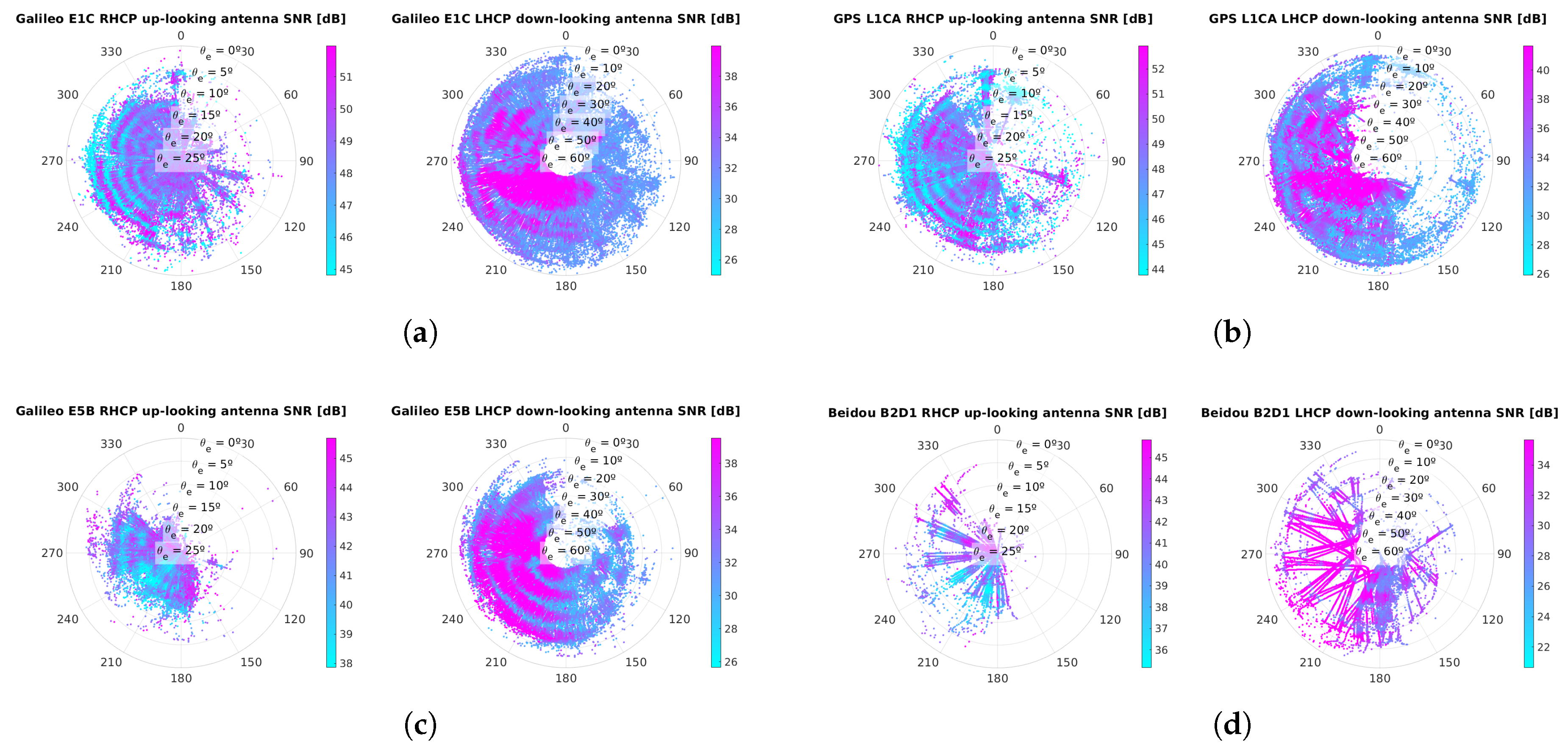
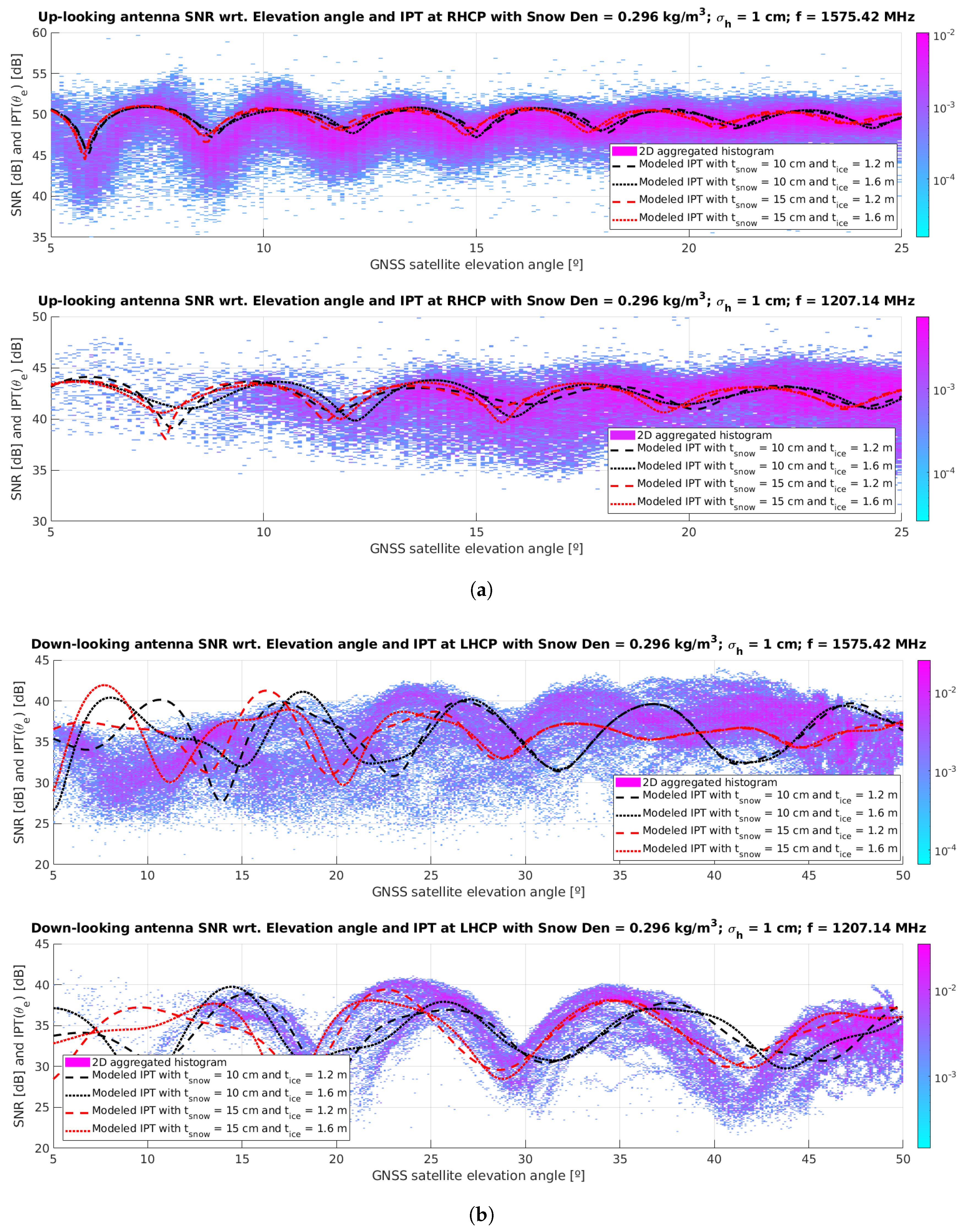
3.2.1. Interference Pattern in the RHCP Zenith-Looking Antenna

This study is focused on two frequencies: 1575.42 MHz, used by GPS L1 C/A code and Galileo E1C; and 1207.14 MHz, used by Galileo E5b and Beidou B2D1 signals. As a first example, the four-layer IP model simulation results are shown in Figure 5a for the up-looking RHCP antenna at 1575.42 MHz for different values of snow, ice thickness, and surface roughness. Note that the antenna heights used to simulate the model are the ones indicated in Figure 2b. Moreover, the contribution to the interference pattern from the reflected path to the up-looking antenna starts to vanish at elevation angles larger than 25° due to the antenna pattern (see Figure 2a). Therefore, the model is only presented up to 30°. Note that the presented IPT is the normalized version of $P\left(\theta \right)$ from Equation (1) (i.e., normalized by $|E_0{|}^2$).

As it can be seen, the position of the different peaks as well as their shape depends on the thickness of the snow layer. The position of both peaks and notches depends mainly on the snow thickness: from 10 to 15 cm thickness, the position of the notches shifts towards the left (lower elevation angles), but for a thicker snow layer (20 cm) the notch position moves towards higher elevation angles (e.g., the notch at 15° of elevation in Figure 5a). In addition, there is also a small dependence on the ice thickness. Comparing the top (ice thickness = 1.2 m) and bottom (ice thickness = 1.6 m) plots in Figure 5a, the notch position is shifted slightly towards lower elevation angles, where thickness variation has less impact in the notch position.

A similar phenomenon happens at 1207.14 MHz (i.e., Galileo E5b and Beidou B2D1) where, depending on both the snow and the ice thickness in the four-layer model, the position where the minima occur fluctuates. As shown in Figure 5b, the four-layer model is also affected by the snow thickness in both the peaks’ shape and the notch position. However, the ice thickness has a larger impact on the notch position as compared to the 1575.42 MHz case as, due to the longer wavelength, the penetration depth into the ice is larger.

Finally, Figure 6 presents a set of curves representing different values of both ice and snow thickness at 1575.42 MHz and 1207.14 MHz. The 1207.14 MHz signal is more sensitive to variations in the ice thickness than to snow thickness (10 to 15 cm), in terms of the positions of peaks and notches. In the 1575.42 MHz case, the nulls’ position in the IP move ∼0.5° in elevation, while in the 1207.14 MHz case they move ∼1.5°.

3.2.2. Interference Pattern in the LHCP Down-Looking Antenna

As the LHCP signal is received by the 45°-tilted down-looking antenna, its reception is not limited by the lower back lobes of the radiation pattern of the RHCP antenna. For this reason, model predictions are presented for elevations from 5° to 60°. Figure 7a presents the IP at LHCP and 1575.42 MHz. Using the same parameters as for the RHCP signal case, the sensitivity to snow thicknesses is even larger than for the RHCP case (Figure 5a). Note that around 30° and 45° of elevation, the ripples produced by the IP have the same shape for different snow thickness, i.e., the curve for 10 cm has the same shape as that for 20 cm, both for an ice thickness of 1.2 m and 1.6 m.

Figure 7b presents the IP at LHCP and 1207.14 MHz. As compared to Figure 5b, the simulated IPs are now sensitive to both ice and snow thickness variations. Comparing both IPs (Figure 7b top and Figure 7b bottom) around 20° of elevation, it can be appreciated that the valleys are modulated by the snow thickness, and their depth (amplitude) and shape depend on the ice thickness.

Comparing the overlaid curves from Figure 7a,b and for different ice thicknesses, in Figure 8 it can be clearly seen that the ice thickness variation does not affect the interference pattern produced between 30° and 42.5° (R2 in Figure 8) of elevation, although at low elevation angles, between 10° and 30°, the IP is sensitive to both snow and ice thickness. Note that, for the sake of simplicity, two ice thickness are shown, but simulations have been carried out for the complete range between 0.6 m. and 1.8 m. with steps of 0.1 m., showing that ice thickness variations are not affecting the interference pattern produced between 30° and 42.5°.

In order to summarize, the IPT with the four-layer model is sensitive to changes in the snow and ice thickness in both RHCP and LHCP signals. However, at 1575.42 MHz, the RHCP has a lower sensitivity to ice thickness. In the 1207.14 MHz case, as the wavelength is longer and thus able to penetrate more into the ice, it shows more sensitivity to ice thickness variations. The LHCP case shows a mixture of both phenomena depending on the elevation angle: for low elevation angles, the IPT is affected by both snow and ice thickness, but for angles between 30° and 42.5°, the IPT mainly depends on the snow thickness. Note that this model does not take into account any antenna orientation, as antenna pattern of the received signal is compensated for.

4. Data Analysis

The PYCARO-2 instrument receives the direct and reflected GNSS signals. In this section, the waveforms’ signal-to-noise ratio (SNR) are presented as radar plots for the different frequencies and constellations. The fringes produced by the reflection geometry can be easily detected by the angle of arrival of the signal (i.e., azimuth and elevation angles).

Figure 9a shows the IPT corresponding to Galileo E1C code, and Figure 9b to the GPS L1 C/A code. It can be clearly identified, in both RHCP signals, where the reflections are coming from, located in the azimuth range from ∼180° to ∼300°. However, in the LHCP signal collected by the down-looking antenna, other interference patterns can be identified in both GPS and Galileo, most of them grouped around 220° and 250°. Moreover, at 1207.14 MHz (Figure 9c,d) Galileo E5B and Beidou B2D1 signals are also exhibiting an IP. It can be seen that the pattern can be appreciated around 210° and 260° of azimuth, whereas for other angles the fringes are slightly changed or even lost.

Because of the antenna pattern of the 45° down-looking antenna, most of the IPs are detected around 220° and 250°, where the fringes are stable at both frequencies. In order to compare the measurements from PYCARO-2 and the four-layer model described in Section 3, the signals have been filtered, and only those received in the 220°–250° of azimuth are used.

In order to ease the visualization of the signal in a 2D form, each SNR measurement retrieved by the instrument has been binned depending on the elevation angle of the transmitting satellite. Each measurement has been divided depending on the receiving antenna (i.e., RHCP or LHCP) and band (1575.42 MHz or 1207.14 MHz). Figure 10 shows, after calibration and azimuth filtering, a 2D histogram of the PYCARO-2 measurements overlaid with the RHCP (a) and the LHCP (b) four-layer model for different snow and ice thicknesses. In order to ease the representation and comparison of the interference pattern, the model curve has been rescaled to have its range in the same span as the PYCARO-2 measurement.

Note that, as seen in the previous section, both snow and ice thickness have an impact on the 1575.42 MHz band. However, it is not large enough to clearly distinguish which model parametrization is closer to the observed pattern. For the 1207.14 MHz case, the number of reflections received for low elevation angles is very small, and therefore, the ripples caused by the interference pattern cannot be clearly identified.

When moving to the LHCP case, as seen in Figure 10b, the retrieved signal is noisier at 1575.42 MHz, where there is only a small range of elevation angles (20° to 35°) with ripples present. However, at 1207.14 MHz, the signal presents notches that can be easily identified as the ones described by the red curve in Figure 10b. In this case, the signal at 1207.14 MHz is able to penetrate deeper into the substrate (i.e., the snow), and therefore it is slightly less sensitive to snow variations. As shown in Figure 3b,c, the snow depth has a larger dispersion than the sea-ice thickness.

4.1. Snow and Ice Thickness Retrievals: Results and Discussion

In order to compare the model and the 2D histogram, the median curve shown in Figure 11 has been computed over a running window with a width of 0.5° in elevation angle. In order to compare those curves and the model, a nonlinear least square (NLS) minimization is performed in different steps. Note that the error function used for the process is the mean-squared error (MSE) of the SNR (dB).

In order to properly retrieve snow and ice thickness, a first NLS minimization is performed for the LHCP signal at elevation angles between 30° and 42.5°, where the minimization parameter is the snow thickness. As seen in the previous section, the LHCP signal around 30° and 42.5° elevation angle is insensitive to ice thickness variations but not to snow thickness variations. In this case, the notch position of the different ripples can be used to estimate the snow thickness.

When the snow thickness is retrieved, a second NLS minimization is performed for the RHCP up-looking signal, between 5° and 25° of elevation. In this second case, the variable used for the second minimization is the ice thickness, using the snow thickness retrieved by the first NLS minimization. Note that in the RHCP case, both snow and ice thickness have an impact on the notch position, and therefore it is very advisable to first retrieve the snow thickness, as in the LHCP case the signal is mainly sensitive to the snow. Moreover, as the RHCP signal is coming from the up-looking antenna, the IPT can only be applied to very low elevation angles, where the antenna pattern has similar values for both the direct and the reflected signal. In this case the reflected signal is also RHCP, as the incidence angle is smaller than the Brewster angle.

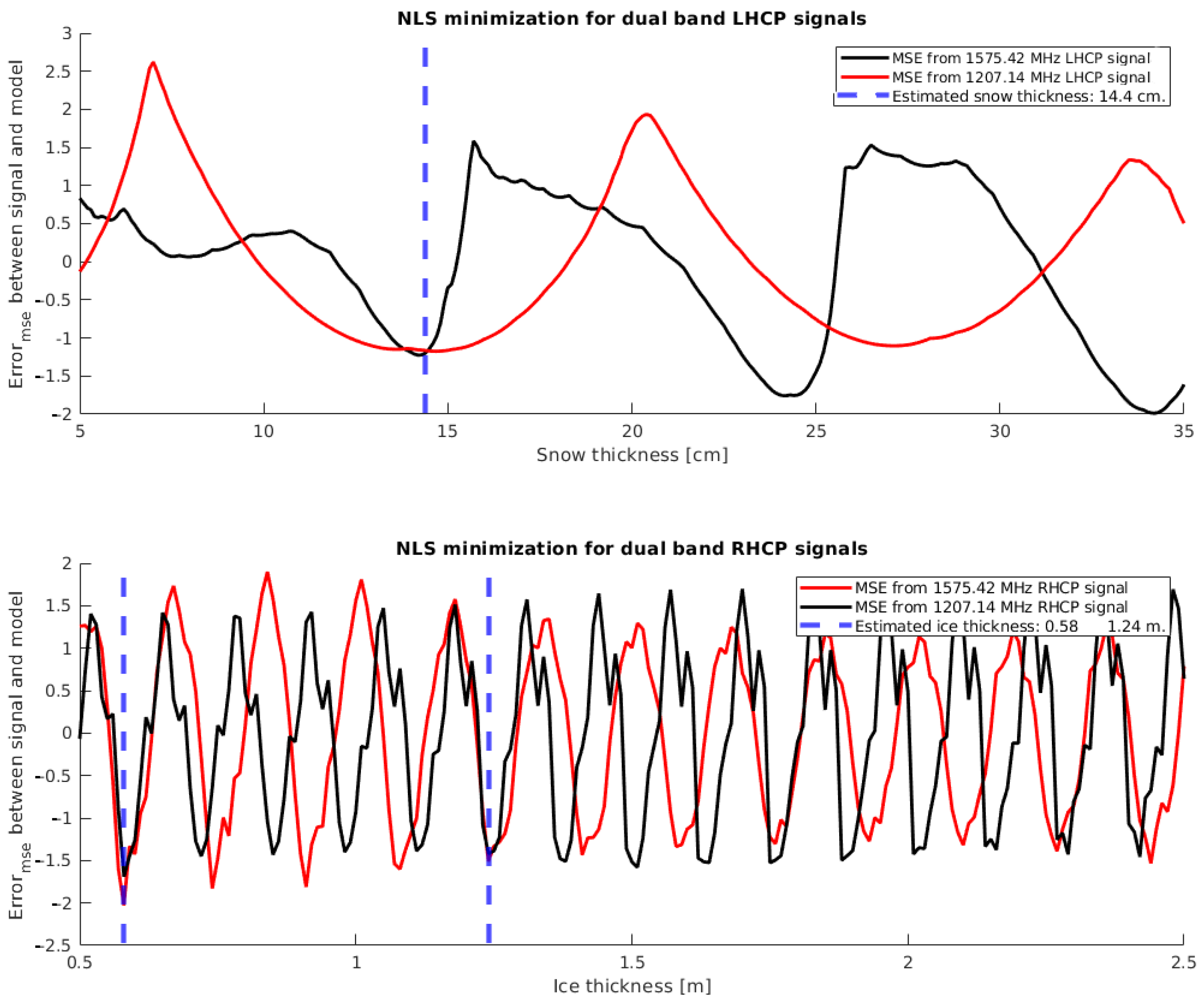
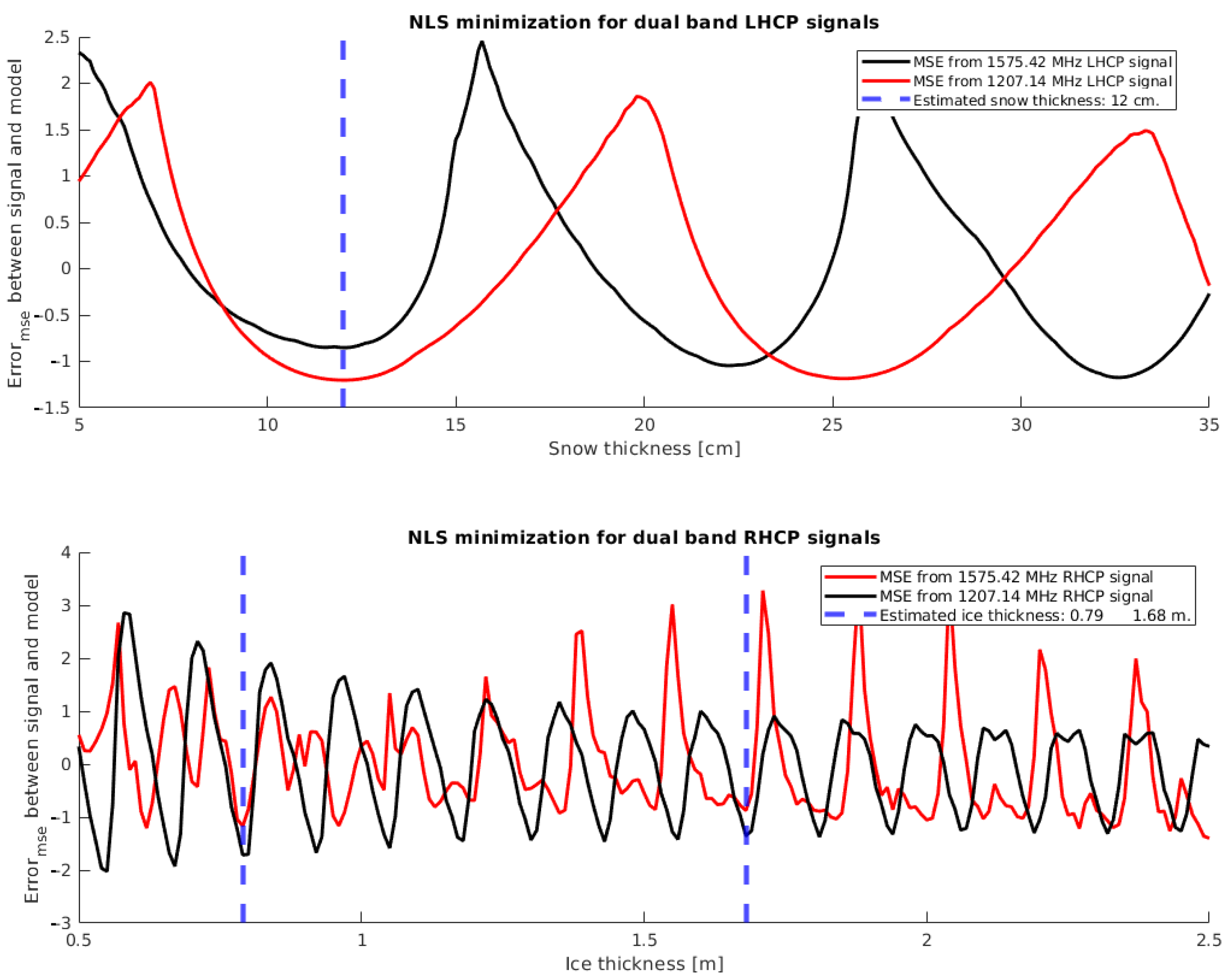
4.1.1. Error Function Analysis and Ambiguity Removal

Both the snow and ice thickness IP produce periodic notches. Therefore, almost equal interference patterns are generated by different combinations of snow and ice thickness. To resolve this uncertainty, data from the two frequency bands (1575.42 MHz and 1207.14 MHz) can be used. The error function with respect to snow and ice thickness is shown in Figure 12. It can be clearly seen that the periodicity of the error function at 1575.42 MHz and 1207.14 MHz are different. In our case, there is a point where both error functions exhibit a minimum at the same time (blue dashed line). This point is the actual snow-ice thickness.

In the case of snow thickness (Figure 12, top), the signal presents a periodicity every 10 cm, and therefore both signals will not present a minimum at the same time in the observation range (i.e., 5 to 35 cm). Therefore, the actual snow thickness can be estimated by overlapping the two normalized error functions. By looking to the sum of both normalized curves, the minimum value is the actual thickness (14.4 cm), which is very close to the measurements by the MOSAiC Remote Sensing team, which were 14.5 ± 0.2 cm.

As for the ice thickness case, as shown in Figure 12 (bottom), a minimum in the MSE function is present every ∼20 cm. Similar to the snow thickness case, the periods are not the same for each band. However, in this case, as the observation range (i.e., 0.5 to 2.5 m) is larger, there are different combinations of thickness values producing a minimum at the same time: 0.58 m. and 1.24 m. Since some a priori knowledge of the ice is required to resolve the ambiguity, we rely on the measured value of 1.21 m on 15 January 2020. Therefore, from both possible solutions, the correct value is likely 1.24 m.

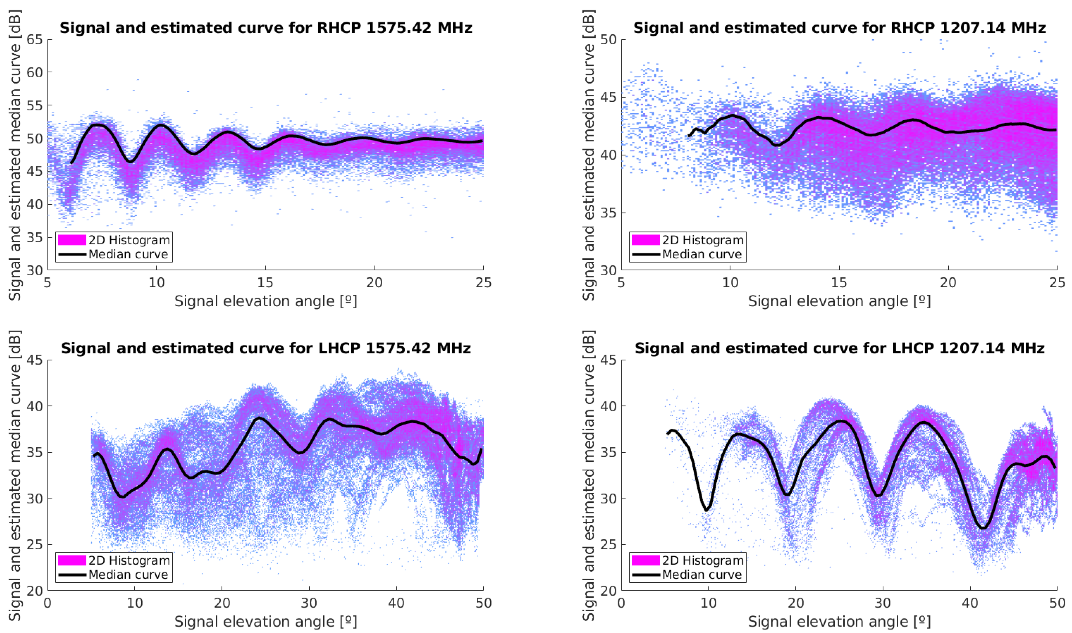
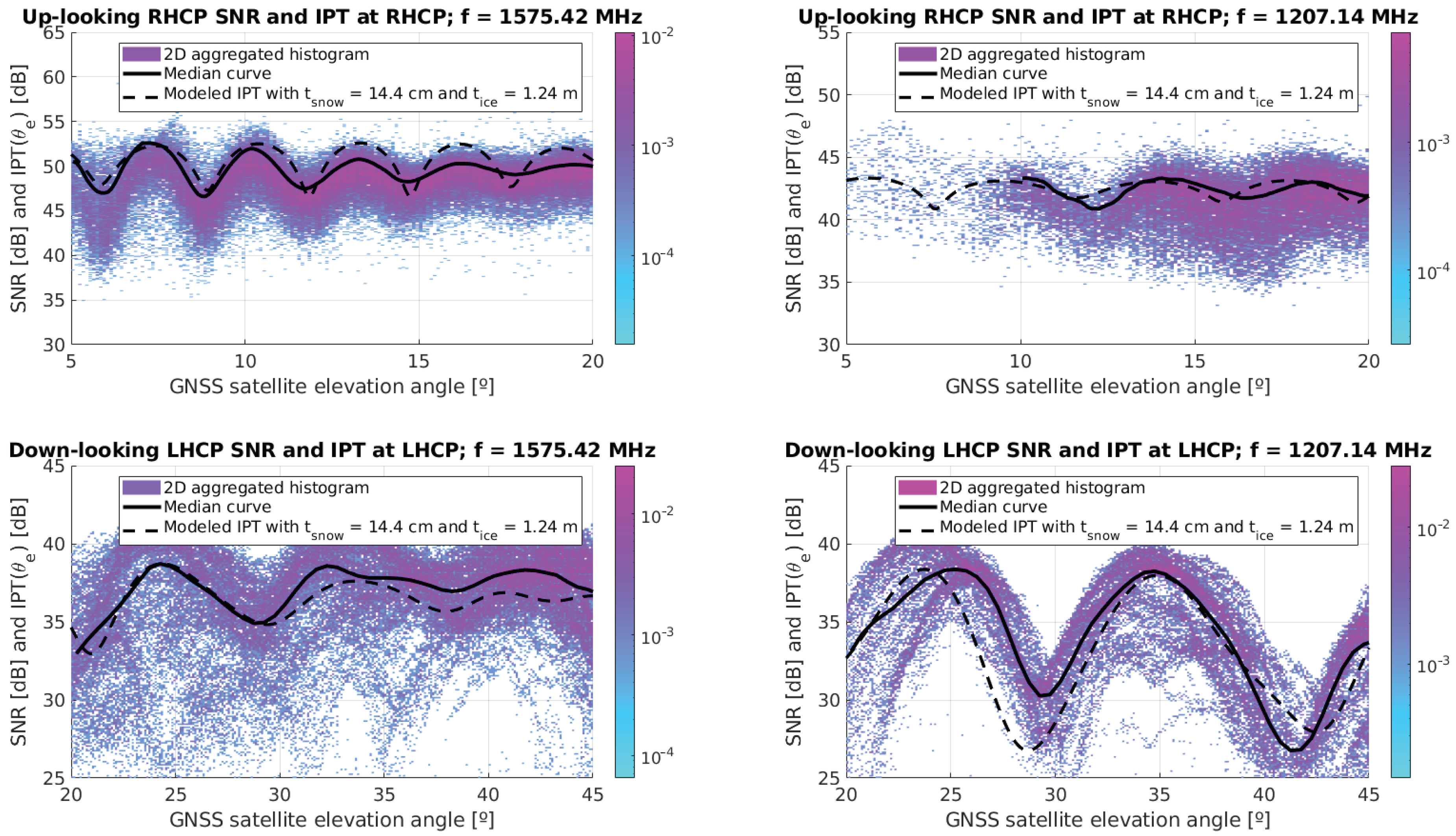
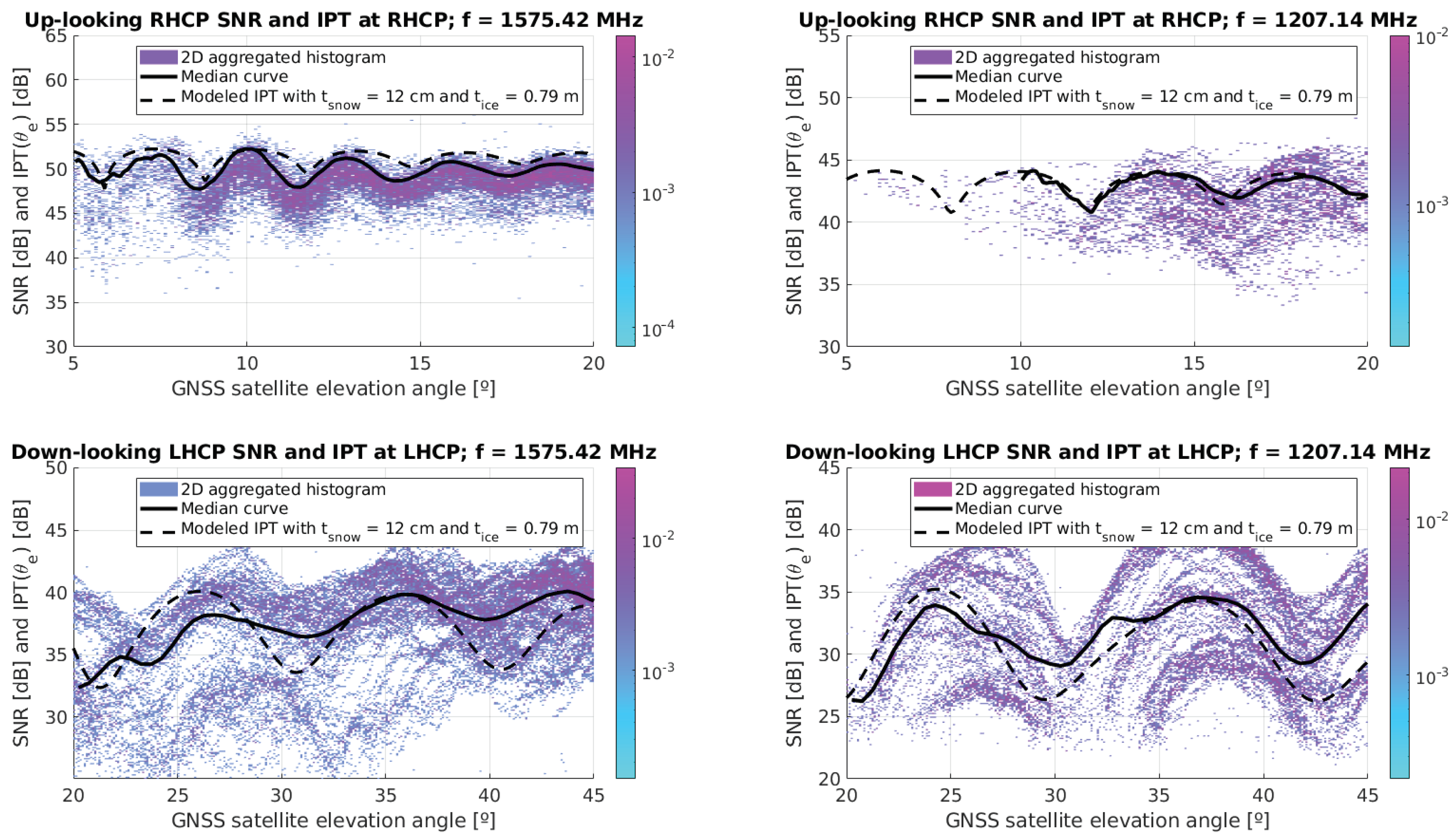
4.1.2. Model and Measured Signal Overlay

Once the thickness parameters have been retrieved, they are used as input for the four-layer IPT model. The modelled IPT is then overlaid on top of the PYCARO-2 data, as shown in Figure 13. Note that the IPT model has been normalized in range (i.e., added a bias and multiplied by a scale factor) in order to better compare it with the SNR values of PYCARO-2.

It can be noticed that the IPT curves are not 100% coincident with PYCARO-2 data in all elevation angles. Despite that, the estimated thickness values are extracted from an MSE minimization process, therefore giving a minimum error for all elevation angles with respect to the median curve used.

Note that in the 1575.42 MHz RHCP signal the notches are also very clear, and therefore we can check that the IPT model and the median curve present the same notches at 6°, 8°, 12°, 14.5°, and 17.5° of elevation angle. In the same way, the median curve and the IPT model for the 1207.14 MHz RHCP signal is presenting two notches at the same position, around 12° and 15.5° of elevation angle.

In order to validate the model for other data sets, another period of data has been used, between the 23rd and 27th of December 2019. In this case, the snow thickness measured from MOSAiC researchers was 11–13 cm, and the estimated ice thickness by means of ice core drilling performed some days before, on 20 December 2019, was around 90 cm. Figure 14 shows the error functions for both ice and snow thickness. In this case, for the minimization process at LHCP, both curves exhibit a minimum at 12 cm of snow thickness, being consistent with the measurements carried out during the campaign. Furthermore, the error curves for RHCP present once more a combination of two values with a minimum of 0.79 m and 1.68 m. In this case, thanks to the knowledge of the actual ice floe thickness, the selected solution is 0.79 m.

The overlaid version is presented in Figure 15. In this case, the notches at 1207.14 MHz, both RHCP and LHCP, are well-matched, as well as the minima and maxima at 1575.42 MHz, LHCP. Despite that, the modeled IPT for the RHCP signal at 1575.42 MHz, and the actual measured data by PYCARO-2 has some mismatch. Even then, the snow and ice thicknesses selected are the ones presenting a minimum MSE between the median curve and the IPT curve.

Even though the estimated ice thickness in this second case differs by 10 cm from the actual measured value, the accuracy of the GEM-2 instrument is 10 cm as well. In addition, as pointed out by the MOSAiC researchers, the ice floe is not evenly growing. To prove that, underwater pictures were taken by a remotely operated vehicle (ROV) during MOSAiC expedition. Furthermore, it is known that small (e.g., 10 cm) and local (meter-scale) undulations are present during the sea-ice freeze up [30], and therefore a single GEM-2 measurement cross-validated using an ice drilling may not be representative of the overall sea-ice thickness but an approximation. It is important to note that this second example of measurements was conducted during December, which is the time period when the ice floe is patched together to form new ice. In this case, some regions may present thinner or thicker spots of ice, which can affect the GNSS-R data measured by PYCARO-2. This phenomena may not be present in the data presented for January, as the different ice sheets have been already merged together.

5. Conclusions

This work has presented the GNSS-R theory and techniques required to estimate the snow and the ice thickness of an ice floe. Multifrequency and dual-polarization GNSS-R can be used to determine both snow and ice thickness by means of the IPT. A peculiarity is that when nonlinear least-square minimization is applied to both RHCP and LHCP signals, it shows a periodicity in the error function, leading to multiple solutions. These uncertainties can be solved by comparing the error functions from different bands. Snow thickness can be easily estimated from this process, as the periodicity of the error with the snow thickness has the same order than the observation range (i.e., a period every 10 cm, observation range ∼40 cm). However, for the ice thickness case, the periodicity of the error with the ice thickness is one order of magnitude smaller than the observation range (i.e., a period every 20 cm, observation range ∼2 m), which leads to multiple solutions for ice thickness that, from the data available for PYCARO-2, cannot be resolved without a priori information. It has been seen that the snow thickness can be more easily retrieved, as it is the one inducing larger changes in the LHCP signal, which led to centimeter errors as compared to the in-situ measurements. However, this is not the case for the ice thickness, where ambiguities may appear, and a priori information is required. Furthermore, it has been seen that the error in the ice thickness retrieval for the second example differs 10 cm from the in-situ measurements.

The interference pattern produced by the four-layer model exhibits some sensitivity to ice thickness variations, especially at the lower frequency band. This means that signals do reflect off the bottom of the ice and reach the air media with still enough power to induce an interference with the direct signal. This behavior supports the hypothesis in [6], from which measurements of the sea ice draft could be possible with GNSS-R. However, there is a wide range of elevation angles where the snow thickness is dominant in the reflection (i.e., between 30° and 42.5° of elevation angle, the ice thickness cannot be measured). In this range of angles, the reflection takes place mostly in the snow-ice interface, while for other elevation angles, the interference pattern is produced in the air-snow, snow-ice, and ice-water interfaces.

From the results presented, it is clearly seen that the snow layer on top of the sea-ice is dominant, while the ice thickness seems to have a smaller impact to GNSS reflections. This phenomena can be also translated to other sensors, where the snow layer shall be properly modeled and taken into account to, for instance, provide an ice thickness measure.

The MOSAiC campaign ended on 30 September 2020, and data from different sensors will be released in the future. For this reason, the acquired data processed through the described algorithm can be used for validation of other MOSAiC instruments such as microwave radiometers. Furthermore, the combination of GNSS-R measurements and measurements from other instruments may increase the accuracy of the GNSS-R retrieved snow and ice thickness, thus helping to remove the ambiguities for different ice thicknesses.

References

1. FSSCat—Towards Federated EO Systems. Available online: https://copernicus-masters.com/winner/ffscat-towards-federated-eo-systems/ (accessed on 29 September 2020).
2. Camps, A.; Golkar, A.; Gutierrez, A.; de Azua, J.R.; Munoz-Martin, J.; Fernandez, L.; Diez, C.; Aguilella, A.; Briatore, S.; Akhtyamov, R.; et al. Fsscat, the 2017 Copernicus Masters’ “Esa Sentinel Small Satellite Challenge” Winner: A Federated Polar and Soil Moisture Tandem Mission Based on 6U Cubesats. In Proceedings of the IGARSS 2018—2018 IEEE International Geoscience and Remote Sensing Symposium, Valencia, Spain, 22–27 July 2018. [Google Scholar]
3. Munoz-Martin, J.F.; Capon, L.F.; de Azua, J.A.R.; Camps, A. The Flexible Microwave Payload-2: A SDR-Based GNSS-Reflectometer and L-Band Radiometer for CubeSats. IEEE J. Sel. Top. Appl. Earth Obs. Remote Sens. 2020, 13, 1298–1311. [Google Scholar] [CrossRef]
4. Alonso-Arroyo, A.; Zavorotny, V.; Camps, A. Sea Ice Detection Using U.K. TDS-1 GNSS-R Data. IEEE Trans. Geosci. Remote Sens. 2017, 1–13. [Google Scholar] [CrossRef] [Green Version]
5. Camps, A. Spatial Resolution in GNSS-R Under Coherent Scattering. IEEE Geosci. Remote Sens. Lett. 2019. [Google Scholar] [CrossRef]
6. Li, W.; Cardellach, E.; Fabra, F.; Rius, A.; Ribó, S.; Martín-Neira, M. First spaceborne phase altimetry over sea ice using TechDemoSat-1 GNSS-R signals. Geophys. Res. Lett. 2017, 44, 8369–8376. [Google Scholar] [CrossRef]
7. Cardellach, E.; Wickert, J.; Baggen, R.; Benito, J.; Camps, A.; Catarino, N.; Chapron, B.; Dielacher, A.; Fabra, F.; Flato, G.; et al. GNSS Transpolar Earth Reflectometry exploriNg System (G-TERN): Mission Concept. IEEE Access 2018, 6, 13980–14018. [Google Scholar] [CrossRef]
8. Kaleschke, L.; Tian-Kunze, X.; Maaß, N.; Mäkynen, M.; Drusch, M. Sea ice thickness retrieval from SMOS brightness temperatures during the Arctic freeze-up period. Geophys. Res. Lett. 2012, 39. [Google Scholar] [CrossRef]
9. European Space Agency. Eight Years of SMOS Arctic Sea Ice Thickness Level Now Available from SMOS Data Dissemination Portal. Available online: https://earth.esa.int/web/guest/missions/esa-operational-eo-missions/smos/news/-/article/eight-years-data-of-smos-arctic-sea-ice-thickness-level-now-available-from-smos-data-dissemination-portal (accessed on 11 November 2019).
10. Carreno-Luengo, H.; Camps, A. First Dual-Band Multiconstellation GNSS-R Scatterometry Experiment Over Boreal Forests From a Stratospheric Balloon. IEEE J. Sel. Top. Appl. Earth Obs. Remote Sens. 2016, 9, 4743–4751. [Google Scholar] [CrossRef] [Green Version]
11. Expedition, M. MOSAiC Expedition Web Page. Available online: https://follow.mosaic-expedition.org/ (accessed on 1 September 2020).
12. Knust, R. Polar Research and Supply Vessel POLARSTERN operated by the Alfred-Wegener-Institute. J. Large-Scale Res. Facil. JLSRF 2017, 3. [Google Scholar] [CrossRef]
13. Munoz-Martin, J.F.; Camps, A.; Cardelach, E.; Pastena, M. Circular Polarization GNSS-R Measurements of MOSAiC RS Site during January 2020. PANGAEA. Available online: https://doi.org/10.1594/PANGAEA924837 (accessed on 15 November 2020).
14. Carreno-Luengo, H.; Amézaga, A.; Vidal, D.; Olivé, R.; Martin, J.M.; Camps, A. First Polarimetric GNSS-R Measurements from a Stratospheric Flight over Boreal Forests. Remote Sens. 2015, 7, 13120–13138. [Google Scholar] [CrossRef] [Green Version]
15. Carreno-Luengo, H.; Camps, A.; Via, P.; Munoz, J.F.; Cortiella, A.; Vidal, D.; Jané, J.; Catarino, N.; Hagenfeldt, M.; Palomo, P.; et al. 3Cat-2 An Experimental Nanosatellite for GNSS-R Earth Observation: Mission Concept and Analysis. IEEE J. Sel. Top. Appl. Earth Obs. Remote Sens. 2016, 9, 4540–4551. [Google Scholar] [CrossRef] [Green Version]
16. Sturm, M.; Holmgren, J. An Automatic Snow Depth Probe for Field Validation Campaigns. Water Resour. Res. 2018, 54, 9695–9701. [Google Scholar] [CrossRef]
17. Hunkeler, P.A.; Hendricks, S.; Hoppmann, M.; Paul, S.; Gerdes, R. Towards an estimation of sub-sea-ice platelet-layer volume with multi-frequency electromagnetic induction sounding. Ann. Glaciol. 2015, 56, 137–146. [Google Scholar] [CrossRef] [Green Version]
18. Rodriguez-Alvarez, N.; Bosch-Lluis, X.; Camps, A.; Vall-llossera, M.; Valencia, E.; Marchan-Hernandez, J.; Ramos-Perez, I. Soil Moisture Retrieval Using GNSS-R Techniques: Experimental Results Over a Bare Soil Field. IEEE Trans. Geosci. Remote Sens. 2009, 47, 3616–3624. [Google Scholar] [CrossRef]
19. Rodriguez-Alvarez, N.; Camps, A.; Vall-llossera, M.; Bosch-Lluis, X.; Monerris, A.; Ramos-Perez, I.; Valencia, E.; Marchan-Hernandez, J.F.; Martinez-Fernandez, J.; Baroncini-Turricchia, G.; et al. Land Geophysical Parameters Retrieval Using the Interference Pattern GNSS-R Technique. IEEE Trans. Geosci. Remote Sens. 2011, 49, 71–84. [Google Scholar] [CrossRef]
20. Rodriguez-Alvarez, N.; Bosch-Lluis, X.; Camps, A.; Aguasca, A.; Vall-llossera, M.; Valencia, E.; Ramos-Perez, I.; Park, H. Review of crop growth and soil moisture monitoring from a ground-based instrument implementing the Interference Pattern GNSS-R Technique. Radio Sci. 2011, 46. [Google Scholar] [CrossRef]
21. Rodriguez-Alvarez, N.; Bosch-Lluis, X.; Camps, A.; Ramos-Perez, I.; Valencia, E.; Park, H.; Vall-llossera, M. Water level monitoring using the interference pattern GNSS-R technique. In Proceedings of the 2011 IEEE International Geoscience and Remote Sensing Symposium, Vancouver, BC, Canada, 24–29 July 2011; pp. 2334–2337. [Google Scholar]
22. Alonso-Arroyo, A.; Camps, A.; Park, H.; Pascual, D.; Onrubia, R.; Martin, F. Retrieval of Significant Wave Height and Mean Sea Surface Level Using the GNSS-R Interference Pattern Technique: Results From a Three-Month Field Campaign. IEEE Trans. Geosci. Remote Sens. 2015, 53, 3198–3209. [Google Scholar] [CrossRef] [Green Version]
23. Rodriguez-Alvarez, N.; Aguasca, A.; Valencia, E.; Bosch-Lluis, X.; Ramos-Perez, I.; Park, H.; Camps, A.; Vall-llossera, M. Snow monitoring using GNSS-R techniques. In Proceedings of the 2011 IEEE International Geoscience and Remote Sensing Symposium, Vancouver, BC, Canada, 24–29 July 2011; pp. 4375–4378. [Google Scholar]
24. Cardellach, E.; Fabra, F.; Rius, A.; Pettinato, S.; D’Addio, S. Characterization of dry-snow sub-structure using GNSS reflected signals. Remote Sens. Environ. 2012, 124, 122–134. [Google Scholar] [CrossRef]
25. Zavorotny, V.U.; Gleason, S.; Cardellach, E.; Camps, A. Tutorial on Remote Sensing Using GNSS Bistatic Radar of Opportunity. IEEE Geosci. Remote Sens. Mag. 2014, 2, 8–45. [Google Scholar] [CrossRef] [Green Version]
26. Kaleschke, L. SMOS Sea Ice Retrieval Study (SMOSSIce): Final Report; ESA ESTEC Contract No: 4000202476/10/NL/CT; Zenodo: Cham, Switzerland, 2013. [Google Scholar] [CrossRef]
27. Vant, M.R.; Ramseier, R.O.; Makios, V. The complex-dielectric constant of sea ice at frequencies in the range 0.1–40 GHz. J. Appl. Phys. 1978, 49, 1264–1280. [Google Scholar] [CrossRef]
28. Lérondel, G.; Romestain, R. Fresnel coefficients of a rough interface. Appl. Phys. Lett. 1999, 74, 2740–2742. [Google Scholar] [CrossRef]
29. Ulaby, F.; Long, D. Microwave Radar and Radiometric Remote Sensing; Artech House: Norwood, MA, USA, 2015. [Google Scholar]
30. Perovich, D.K.; Grenfell, T.C.; Richter-Menge, J.A.; Light, B.; Tucker, W.B., III; Eicken, H. Thin and thinner: Sea ice mass balance measurements during SHEBA. J. Geophys. Res. Ocean. 2003, 108. [Google Scholar] [CrossRef]
Figure 1. IEEC’s GNSS-R instruments: IEEC-ICE/CSIC GNSS-R instrument is formed by the zenith antenna and by the 5 × 1 patch array pointing to the horizon. IEEC/CTE-UPC GNSS-R instrument is formed by the zenith antenna and the 45° incidence angle LHCP antenna. [Credits: Gunnar Spreen].
Remotesensing 12 04038 g001
Figure 2. (a) Up-looking and down-looking antenna pattern; (b) antenna distribution and heights of each antenna; (c) MOSAIC Remote Sensing site with GNSS-R instruments (orange arrow), and (d) MOSAiC ice cracks during November–December 2019 [Credits: Gunnar Spreen and Stefan Hendricks].
Remotesensing 12 04038 g002
Figure 3. (a) Avalanche probe measurements in the vicinity of the GNSS-R instrument; (b) Snow depth and (c) Sea-ice thickness PDF for different dates in the level ice area adjacent to Remote Sensing site measured by Magnaprobe and GEM-2.
Remotesensing 12 04038 g003
Figure 4. Four-model layer applied to PYCARO-2 instrument in MOSAiC campaign.
Remotesensing 12 04038 g004
Figure 5. Four-layer model at RHCP for five different snow layer thickness at two predefined ice thickness, (top) 1.2 m, and (bottom) 1.6 m. Simulation at 1575.42 MHz (a) and 1207.14 MHz (b). Assuming a surface roughness between layers of 1 cm.
Remotesensing 12 04038 g005
Figure 6. Comparison of the RHCP four-layer model at 1575.42 MHz (top) and 1207.14 MHz (bottom), using four different combinations of snow and ice thickness.
Remotesensing 12 04038 g006
Figure 7. Four-layer model at LHCP for five different snow thickness, at two predefined ice thickness, 1.2 m (top), and 1.6 m (bottom). Simulation at 1575.42 MHz (a) and 1207.14 MHz (b). Assuming a surface roughness of 1 cm.
Remotesensing 12 04038 g007
Figure 8. Comparison of the LHCP four-layer model at 1575.42 MHz and 1207.14 MHz, using four different combinations of snow and ice thickness. IPT in region 1 (R1) is affected by ice and snow thickness, while IPT in region 2 (R2) is unaffected by ice-thickness variations.
Remotesensing 12 04038 g008
Figure 9. Radar plot of the SNR for (a) Galileo E1C, (b) GPS L1 C/A, (c) Galileo E5b signal, and (d) Beidou B2D1 during January 2020.
Remotesensing 12 04038 g009
Figure 10. Aggregated 2D histogram (density plot) for the up-looking RHCP signal SNR for both 1575.42 MHZ and 1207.14 MHz; and IPT for RHCP (a) and LHCP (b) signal for different snow and ice thickness.
Remotesensing 12 04038 g010
Figure 11. 2D histograms (density plot) and median curve (in black) for the received signals in GPS L1 C/A, Galileo E1C, Galileo E5b, and Beidou B2D1.
Remotesensing 12 04038 g011
Figure 12. NLS minimization output for the data set between the 15th and the 27th of January 2020. MSE is represented for both snow and ice thickness, for different signal frequencies and polarization, and it has been normalized (z-score normalization) to ease its visualization. Note that the exact place where both signals present a minimum at the same thickness is represented by the blue dashed line thickness and the ice thickness have an impact on the notch positions; therefore, it is very advisable to first retrieve the snow thickness. As in the LHCP case, the signal is mainly sensitive to the snow.
Remotesensing 12 04038 g012
Figure 13. Modeled IPT using the retrieved snow and ice thickness overlaid on top of the signal retrieved by the PYCARO-2 instrument in the MOSAiC campaign during January 2020. Both the median curves and the modeled interference patterns are represented in black.
Remotesensing 12 04038 g013
Figure 14. NLS minimization output for the data set between the 23rd and the 27th of December 2019. MSE is represented for both snow and ice thickness, for different frequencies and signal polarization, and it has been normalized (z-score normalization) to ease its visualization. Note that the blue-dashed line shows the exact thickness at which both signals present a minimum.
Remotesensing 12 04038 g014
Figure 15. Modeled IPT using the retrieved snow and ice thickness overlaid on top of the signals retrieved by the PYCARO-2 instrument in the MOSAiC campaign during December 2019. Both the median curves and the modeled interference patterns are represented in black.
Remotesensing 12 04038 g015
Publisher’s Note: MDPI stays neutral with regard to jurisdictional claims in published maps and institutional affiliations.