Article

An Edge-Sense Bidirectional Pyramid Network for Stereo Matching of VHR Remote Sensing Images

1
Aerospace Information Research Institute, Chinese Academy of Sciences, Beijing 100190, China
2
School of Electronic, Electrical and Communication Engineering, University of Chinese Academy of Sciences, Huairou District, Beijing 101408, China
3
Key Laboratory of Technology in Geo-Spatial Information Processing and Application System, Chinese Academy of Sciences, Beijing 100190, China
*
Author to whom correspondence should be addressed.
Remote Sens. 2020, 12(24), 4025; https://doi.org/10.3390/rs12244025
Submission received: 2 November 2020 / Revised: 30 November 2020 / Accepted: 5 December 2020 / Published: 9 December 2020
(This article belongs to the Section Remote Sensing Image Processing)

Abstract

:
As an essential step in 3D reconstruction, stereo matching still faces unignorable problems due to the high resolution and complex structures of remote sensing images. Especially in occluded areas of tall buildings and textureless areas of waters and woods, precise disparity estimation has become a difficult but important task. In this paper, we develop a novel edge-sense bidirectional pyramid stereo matching network to solve the aforementioned problems. The cost volume is constructed from negative to positive disparities since the disparity range in remote sensing images varies greatly and traditional deep learning networks only work well for positive disparities. Then, the occlusion-aware maps based on the forward-backward consistency assumption are applied to reduce the influence of the occluded area. Moreover, we design an edge-sense smoothness loss to improve the performance of textureless areas while maintaining the main structure. The proposed network is compared with two baselines. The experimental results show that our proposed method outperforms two methods, DenseMapNet and PSMNet, in terms of averaged endpoint error (EPE) and the fraction of erroneous pixels (D1), and the improvements in occluded and textureless areas are significant.

Graphical Abstract

1. Introduction

With the rapid growth of remote sensing image resolution and data volume, the way we observe the Earth is no longer limited to two-dimensional images. Multiview remote sensing images acquired from different angles provide the foundation to reconstruct the three-dimensional structures of the world. 3D reconstruction from multiview remote sensing images has been applied to various fields including urban modeling, environment research, and geographic information systems. As the essential step of 3D reconstruction, stereo matching finds dense correspondences from a pair of rectified stereo images, resulting in pixelwise disparities. Disparities refer to the horizontal displacement between the corresponding points ( ( x , y ) in the left image, ( x d , y ) in the right image), which can be directly used to calculate height information.
Traditionally, stereo matching algorithms can be divided into four steps: matching cost computation, cost aggregation, cost optimization, and disparity refinement [1]. Feature vectors extracted from each image are used to calculate the matching cost. However, without the cost aggregation, the matching results are usually ambiguous on account of the weak features in occluded, textureless, and noise-filled areas. The Semi-Global Matching (SGM) algorithm [2], which optimizes the global energy function with aggregation in many directions, is the most widely used method for cost aggregation. Several improvements of the SGM method have been proposed by designing more robust matching cost functions [3,4].
Recently, with the rapid application of deep learning methods, the convolutional neural network (CNN) has been applied to match the points combining deep feature representation with the traditional following steps. Some methods focus on computing accurate matching cost by CNN and apply the SGM and other traditional methods to refine the disparity map. For example, the MC-CNN [5], proposed by Zbontar and LeCun, used a Siamese network to learn the similarity measure by binary classifying the image patch data. After computing the matching cost using a pair of 9 × 9 , the network uses the traditional cost aggregation, SGM, and disparity refinements to further improve the quality of the matching results. Luo et al. [6] proposed a faster Siamese network to compute the matching cost by treating the procedure as a multilabel classification. Some other studies focus on the postprocessing of the disparity map. Displets [7] used the 3D models to solve the matching cost computation in textureless areas. SGM-Net [8] made it so that the SGM penalties can be learned by network instead of manually tuning the parameters.
However, the methods combining the CNNs and traditional cost aggregation and disparity refinement often predict ambiguous disparity in textureless areas. Consequently, end-to-end deep neural networks have been developed to incorporate the global context information with the four steps and obviously show more progress than the traditional algorithms. The first end-to-end stereo matching network (DispNet [9]) was trained by a large synthetic dataset. Cascade residual learning (CRL) [10] was proposed to match stereo pairs using a two-stage network. The DispNet and CRL both exploit hierarchical information from multiscale features. GC-Net [11] first used the 3D encoder–decoder convolutions to refine cost volume in cost aggregation. In a more recent work, PSMNet [12], a pyramid stereo matching network, applied SPP (spatial pyramid pooling) to enlarge the reception fields and applied the stacked hourglass network to increase the number of 3D convolution layers, which further improved the performance. It learned the experience from semantic segmentation and built a multiscale pyramid context aggregation for depth estimation.
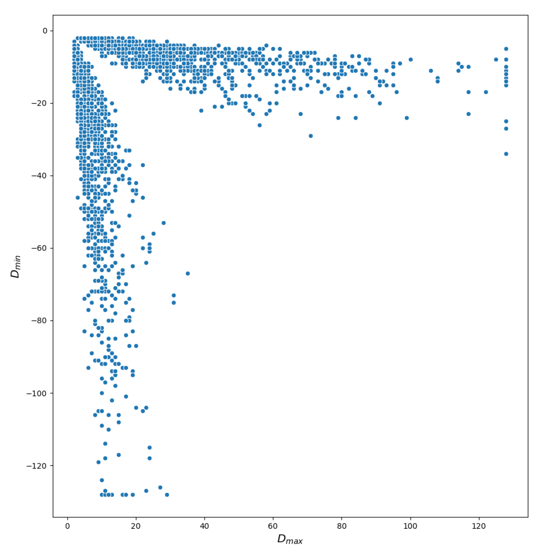
Despite the growing resolution of remote sensing images, multiview high resolution (VHR) remote sensing images are more complicated compared to the stereo images acquired from frame cameras. First, due to different viewing angles, the disparities in remote sensing stereo pairs contain both positive and negative values. As shown in Figure 1, we gathered the max and min disparities of each truth DSP (disparity map) in IGARSS2019 data fusion contest dataset US3D. Second, there exist numerous occluded areas in the urban regions, and it is difficult to obtain accurate correspondences in some areas such as waters and woods since they present repetitive patterns and few textures. Last, disparities in multiview remote sensing images with large scenes show great diversity since they contain complex and multiscale structures, which increase the difficulty to construct the cost volume.
In order to solve the aforementioned problems in stereo matching on multiview remote sensing images and improve the performance of deep learning networks, in this paper, we propose a novel edge-sense bidirectional pyramid stereo matching network. Considering the property that disparity in remote sensing images varies greatly, we reconstruct the cost volume to cover both positive and negative disparities. To obtain bidirectional occlusion maps, we stack the stereo pairs to predict the disparities in both the left-to-right and right-to-left directions. By adopting the forward-backward consistency assumption in traditional optical flow framework [13,14], we combine the unsupervised bidirectional loss [15] with the supervised loss function to ensure the accuracy of disparity estimation. Moreover, aiming at improving the performance in the textureless regions while maintaining the main structure, we proposed an edge-sense second-order smoothness loss to optimize the network.
The main contributions of our work can be summarized in three points: (1) we reconstruct the cost volume and reset the range of disparity regression to estimate both positive and negative disparity maps in remote sensing images; (2) we present a bidirectional unsupervised loss to solve the disparity estimation in occluded areas; (3) we propose an edge-sense smoothness loss to improve the performance in the textureless regions without blurring the main structure.

2. Methodology

In this section, the whole structure of our proposed network is illustrated first. Then, the reconstruction of cost volume is introduced. Moreover, we show the details of implementing the training loss including supervised loss, bidirectional unsupervised loss, and edge-sense smoothness loss.

2.1. The Architecture of the Proposed Network

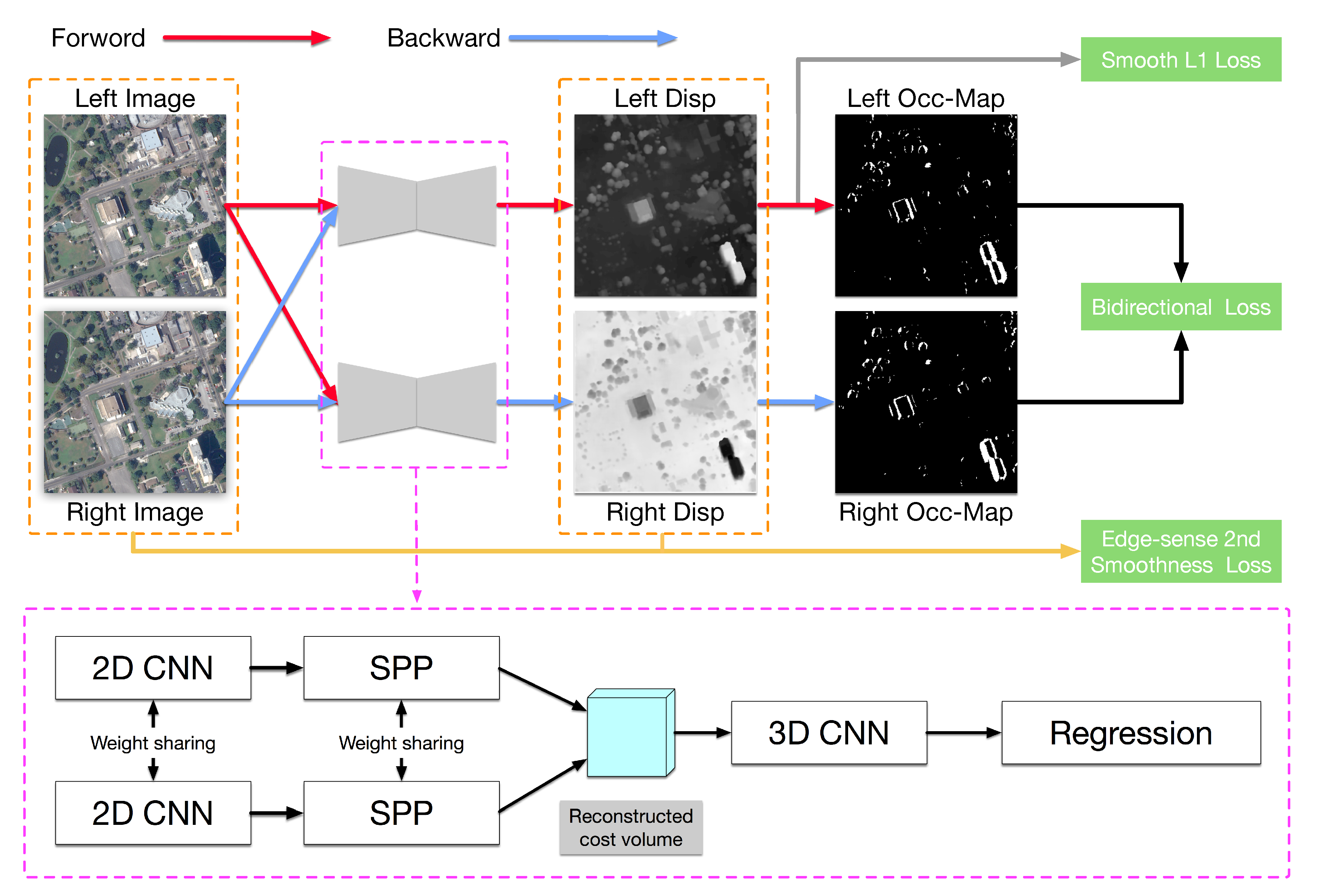
We propose an edge-sense bidirectional pyramid stereo matching network for the disparity estimation of rectified remote sensing pairs. The overall architecture of the proposed network is shown in Figure 2. First, considering that both positive and negative disparities exist in multiview remote sensing images, we modify the construction of cost volume and disparity regression. Then, aiming at obtaining the bidirectional occlusion-aware maps, the stacked stereo pairs are fed into the Siamese network based on the reconstructed cost volume. We adopt the same feature extraction layers (2D CNN and SPP) as PSMNet [12] in each branch, which are used to exploit global context information. Moreover, the stacked hourglass module is applied in the cost volume regularization to estimate disparity.
The network is optimized by both the supervised loss and unsupervised bidirectional loss. As for the supervised term, we adopted the smooth L 1 loss to train the network, which is widely used in many applications because of its robustness. Aiming at generating the bidirectional occlusion map, the forward disparity map and the backward one are estimated by the stereo pair and the reverse pair, respectively. Then, the bidirectional disparity maps are used to generate the occlusion-aware maps, which refer to the forward-backward consistency assumption. Finally, we introduce the edge information extracted from the stereo images into the second-order smoothness loss to improve results in textureless regions. Overall, combining the weighted bidirectional occlusion map loss and the second-order smoothness loss with the edge prior, the proposed network, named Bidir-EPNet, can present robust performance both in structural and textureless areas.

2.2. Construction of the Cost Volume

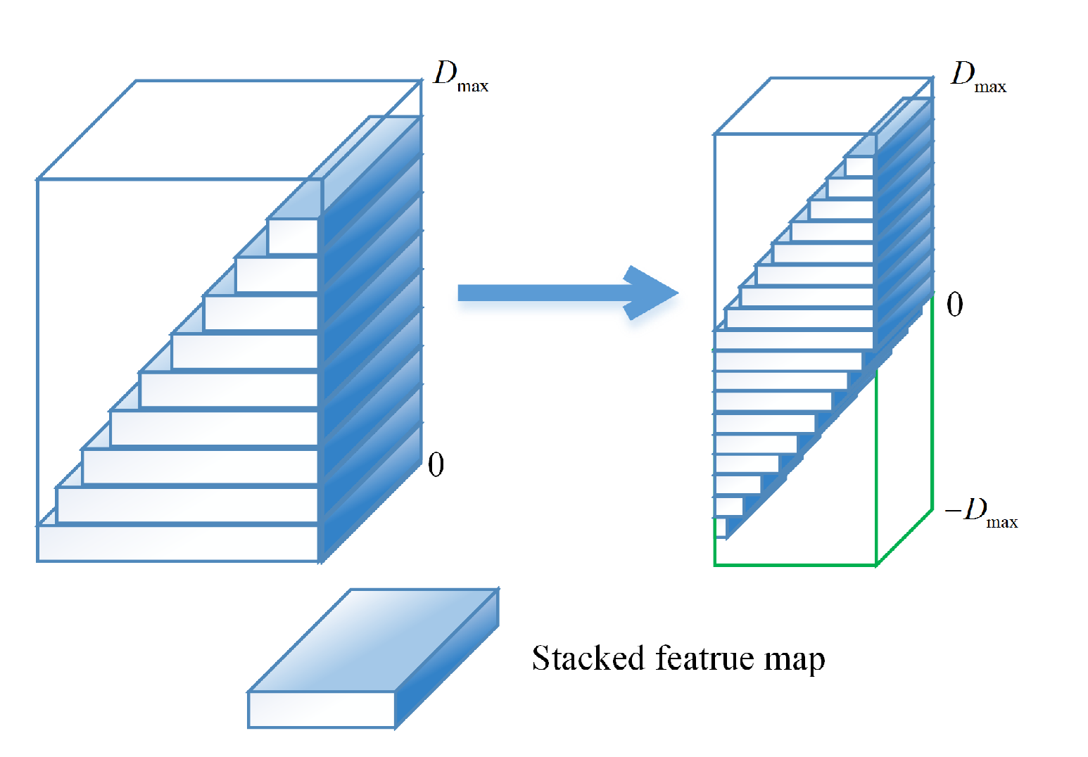
Since the disparities in remote sensing images vary greatly (as shown in Figure 1), we stack the input stereo image pair and the corresponding inverse pair to generate bidirectional disparity maps. In order to estimate the disparity accurately using the stacked stereo pairs, the cost volume and its disparity regression range need to be reset. The cost volume is constructed by concatenating the left feature with their corresponding right feature across each disparity level [11,12]. The disparity regression algorithm, proposed in [11], is applied to estimate the continuous disparity map. The predicted disparity d ^ can be calculated by the sum of d weighted by their predicted probability via softmax operation σ · . In this paper, the cost volume is reconstructed with the range of [ D m a x , D m a x ] , as shown in Figure 3. Consequently, the corresponding disparity regression range is reset to [ D m a x , D m a x ] and the predicted disparity d ^ can be calculated as follows:
d ^ = d = 0 D m a x d × σ ( s o f t m a x ( d ) ) .
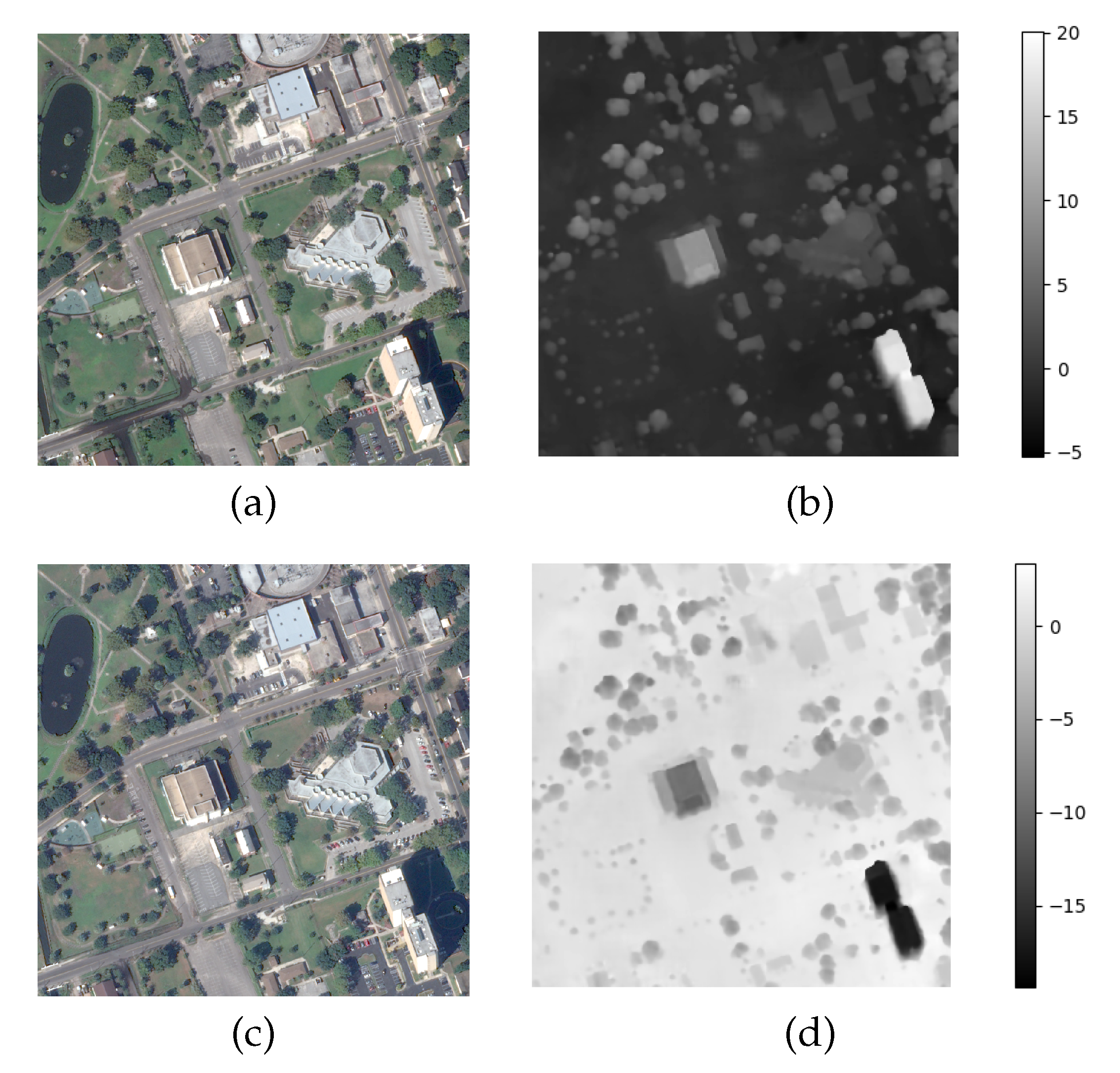
Using the bidirectional cost volume, the proposed network can generate bidirectional disparity maps simultaneously. Two examples of bidirectional disparity maps based on left and right stereo images are shown in Figure 4.

2.3. Training Loss

2.3.1. The Supervised Training Loss

In this paper, we first adopt the smooth L 1 loss as the supervised loss to train the Bidir-EPNet to generate the initial disparity maps. Smooth L 1 loss has proved its robustness to outliers in disparity estimation [16], compared to the L 1 term. The supervised loss function used in this network is the same as the PSMNet, which is given as follows:
L ( d , d ^ ) = 1 N i = 1 N s m o o t h L 1 ( d i d ^ i ) ,
where
s m o o t h L 1 ( x ) = { x 2 / 2 , if | x | < 1 | x | 0.5 , otherwise
where N is the valid number of pixels labeled by ground truth and d d ^ represents the difference between ground truth and predicted disparity.

2.3.2. The Unsupervised Bidirectional Loss

Aiming at reducing the deformation produced by noncorresponding pixels in such occluded regions, the occlusion-aware map, which masks out the occluded pixels, is taken into account. Inspired by the traditional optical flow methods, an unsupervised loss based on the classical brightness forward-backward consistency and smoothness assumptions is proposed to predict optical flow [15]. Since stereo matching is a special case of optical flow estimation, we adopt the forward-backward consistency assumption in the traditional optical flow framework to further refine the disparity maps. Similar to the UnFlow [15], we extend this method to apply the occlusion-aware unsupervised loss to estimate bidirectional disparity.
Let I 1 , I 2 be the left and right patch in stereo pair. Our goal is to predict the disparity d f ( x ) from I 1 to I 2 , whereas the backward disparity from I 2 to I 1 is d b ( x ) . The occluded areas are detected based on the forward-backward consistency assumption. The basic observation of the assumption is that a pixel in the left image should correspond to the pixel mapped by the forward and backward disparities. Based on this assumption, the distance of forward-backward disparities should be zero for accurate correspondences. We then mask the occluded areas, where the corresponding pixel is not visible, by comparing the distance with a given threshold. To be specific, the constraint of occluded areas detection is given as:
o f : | d f ( x ) + d b ( x + d f ( x ) ) | 2 < α 1 | d f ( x ) | 2 + | d b ( x + d f ( x ) ) | 2 + α 2 , o b : | d b ( x ) + d f ( x + d b ( x ) ) | 2 < α 1 | d b ( x ) | 2 + | d f ( x + d b ( x ) ) | 2 + α 2 ,
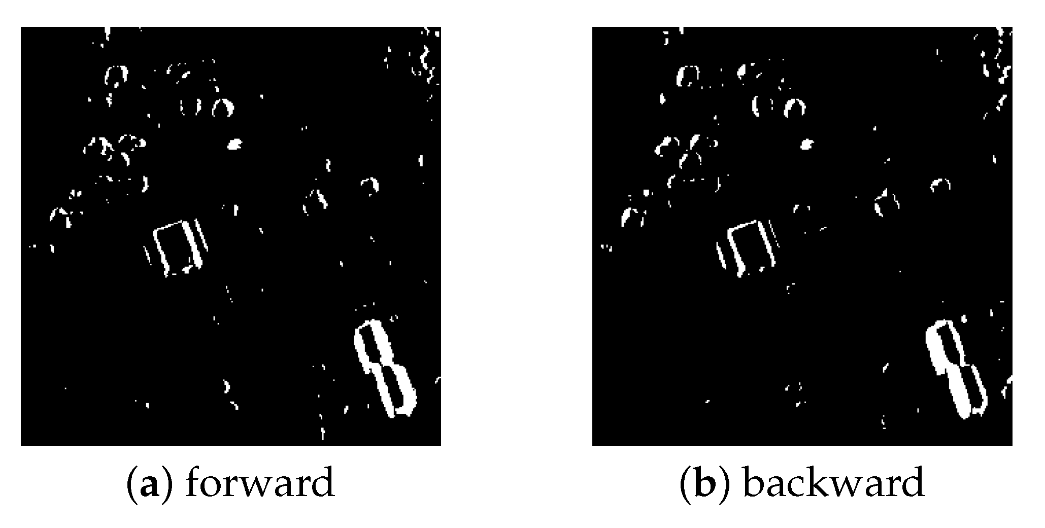
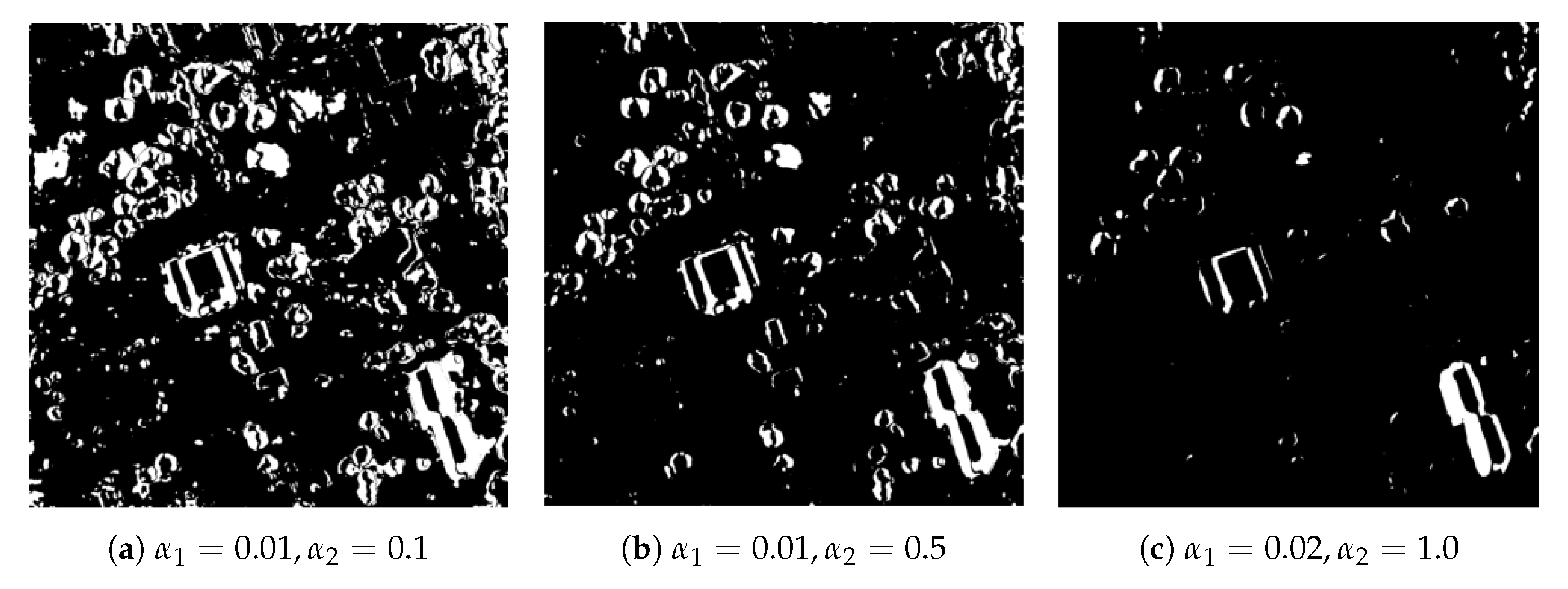
where d f , o f represent the forward disparity and occlusion map based on the left image and d b , o b represent the backward disparity and occlusion map based on the right image. We set the parameters α 1 = 0.02 , α 2 = 1.0 to generate a more concentrated area for VHR satellite images, and let o f = 0 when the constraint is maintained. The backward occlusion map is then obtained by changing the order of d f and d b .
After generating the bidirectional occlusion-aware maps (shown in Figure 5), the unsupervised bidirectional loss is defined as:
E b i d i r ( d f , d b , o f , o b ) = x P ( 1 o f ) · ρ f D ( I 1 ( x ) , I 2 ( x + d f ( x ) ) ) + ( 1 o b ) · ρ f D ( I 2 ( x ) , I 1 ( x + d b ( x ) ) ) ,
where I ( x ) represents the left image and I ( x + d f ( x ) ) represents the backward warped right image via forward disparity map. To apply a differentiable way for backpropagation, we use the bilinear sampling scheme to warp the image. ρ ( x ) = ( x 2 + ϵ 2 ) γ is a robust Charbonnier penalty function [17] with γ = 0.45 , and f D ( I 1 ( x ) , I 2 ( x ) ) = I 1 ( x ) I 2 ( x ) can measure the photometric difference between two corresponding point in stereo pairs based on the brightness constancy constraint.

2.3.3. The Edge-Sense Second-Order Smoothness Loss

Considering that the untextured feature in some flat regions such as water and woods produces ambiguous disparities, the smoothness operation is used. The second-order smoothness function defined on eight-pixel neighborhoods in three directions, S ( q , p , r ) = D ( p ) 2 D ( q ) + D ( r ) 1 , is used both in stereo matching and optical flow regularization [18] since it can maintain the collinearity of neighborhoods. However, simply applying the second-order smoothness term may blur the sharp structures in urban areas. Consequently, we choose the Laplacian function defined on four- or eight-pixel image neighborhoods to maintain thin structures along with edge directions. Inspired from [19], in order to preserve sharp edge information, we combine the original smoothness loss via bidirectional disparity maps and the edge-sense previously computed by the image intensity.
In order to retain the accurate disparities across edges, the second derivative of the image I ( s ) 2 I ( x ) + I ( r ) 1 is utilized as the weight of the smoothness term. Therefore, the edge-sense second-order smoothness loss and the weighted edge prior are defined as:
E s ( x ) = 1 3 w ( x , { s , r } ) · E ( x , { s , r } ) , 1 3 w ( x , { s , r } ) · E ( x , { s , r } ) < 0.3 0.3 ,      1 3 w ( x , { s , r } ) · E ( x , { s , r } ) 0.3 ,
where
w ( x , { s , r } ) = exp I ( s ) 2 I ( x ) + I ( r ) 1 γ , E ( x , { s , r } ) = x P ( s , r ) N ( x ) ρ d f ( s ) 2 d f ( x ) + d f ( r ) + ρ d b ( s ) 2 d b ( x ) + d b ( r ) ,
where N ( x ) represents the eight-pixel neighborhood, · is L 1 normal of a vector, and I ( x ) is the intensity at the center pixel x, and the weight term w ( x ) denotes edge intensity at x, which is controlled by the parameter γ . It is clear that the w ( x ) and E ( x ) become zero along edge direction. Therefore, the disparity information in edge regions is less affected by the smoothness term.
Aiming at smoothing the disparities along multiple directions, we extract edge maps from three different directions (horizontal, vertical, and diagonal). Then, we sum different responses from these directions and normalize them to [ 0 , 1 ] . Finally, we simply use a clipping threshold of 0.3 to capture more specific edge information.
In conclusion, our final loss function is the weighted combination of supervised smooth L 1 loss, the bidirectional unsupervised loss, and the edge-sense second-order smoothness loss; the three parameters λ 1 , λ 2 , λ 3 are the weights for each loss function, respectively.
E a l l = λ 1 E s m o o t h L 1 + λ 2 E b i d i r + λ 3 E s .

3. Experimental Results

In this section, we first introduce the dataset description, implementation details, and quantitative metrics for assessment. Then, quantitative and qualitative results are presented to evaluate the performance of the proposed network.

3.1. Datasets and Experimental Parameter Settings

The track2 dataset US3D of 2019 IEEE Data Fusion Contest [20,21] is used to evaluate the network performance. The dataset consists of 69 VHR multiview images collected by WorldView-3 between 2014 and 2016 over Jacksonville and Omaha in the United States of America, which contain various landscapes such as skyscrapers, residential buildings, rivers, and woods. The stereo pairs in this dataset are rectified in a size of 1024 × 1024 and are geographically nonoverlapped. In order to evaluate our proposed network, two baselines, PSMNet [12] and DenseMapNet [22], are compared. Two quantitative metrics, the averaged endpoint error (EPE) and the fraction of erroneous pixels (D1), are used to assess the performance.
We use the tiled stereo pairs from Jacksonville to train our model, while the pairs from Omaha are used to test in order to verify the generalization of the proposed network. Table 1 shows the configurations of datasets in detail. We have chosen 1500 stereo pairs from different scenes in Jacksonville (JAX) as the training dataset, while the remaining 346 pairs in JAX and the whole Omaha (OMA) pairs are used for testing. Moreover, we train the proposed Bidir-EPNet with the Adam optimizer configuring β 1 = 0.9 , β 2 = 0.999 . The input stereo image pairs are randomly cropped into H = 512 and W = 512 . The total epoch is set to 300. While training, the learning rate is set to 0.01 for the former 200 epochs and 0.001 for the remaining 100 epochs. The image intensity is normalized into [ 0 , 1 ] in order to eliminate the radiometric difference. The batch size is set to 8 on two NVIDIA Titan-RTX GPUs. All the experiments are implemented on a Ubuntu18.04 OS with PyTorch environment.
Herein, aiming at evaluating the performance of the proposed network, we train the network on 1500 training stereo pairs in JAX and test on the remaining 346 pairs in the JAX and OMA pairs. First, for the generation of the bidirectional occlusion-aware maps, we stark the input stereo pairs and the reverse one with batchsize 8. Then, the cost volume and disparity regression range is set to [ 64 , 64 ] . For the term of bidirectional data loss, the two parameters α 1 , α 2 controlling the threshold in forward-backward assumption are reset to 0.02 and 1.0, respectively, considering the inherent property of VHR remote sensing images. Then, for the edge-sense second-order smoothness loss, we extract edge information from three directions—horizontal, vertical, and diagonal—to weight the second-order smoothness loss. The edge significance controlled parameter γ is set to 20. Finally, as for the weighted parameters in smooth L 1 loss, we adopt the three weight values of the stacked hourglass network, 0.5, 0.7, and 1.0, for Loss_1, Loss_2, and Loss_3, respectively, following the default settings in PSMNet. For balancing the three training losses, λ 1 , λ 2 , and   λ 3 in our final loss function are set to 1.0, 0.5, and 0.8, respectively.

3.2. Results

In order to assess the performance of the proposed network, two quantitative metrics, EPE (pixel) and D1 (%), are used to compare the disparity estimation precision between the three networks. The averaged endpoint error (EPE) is defined by E P E ( d d ^ ) = d d ^ 2 . A pixel is marked as an erroneous pixel when its absolute disparity error is larger than t pixels and the fraction of erroneous pixels in all valid areas is called D1. Note that t is set to 3 in general. As a result, Table 2 shows the quantitative evaluation results of the three algorithms on both the JAX test dataset and the whole OMA images. It is clear that the proposed network gives the best results, and on JAX it raises by about 6% and 15% in terms of EPE and D1 compared to the PSMNet. Moreover, the quantitative results also illustrate better generalization of the proposed network by raising about 2% in terms of both EPE and D1 compared to PSMNet. Subsequently, to show the improvements on such occluded and textureless regions, several stereo pairs containing some typical scenes such as tall buildings and waters are assessed both in quantitative and visual results.

3.2.1. Results on Occluded Areas

To assess the performance of our network in some occluded areas, we choose five significant stereo pairs that contain these occluded regions including tall buildings (as shown in Figure 6). Table 3 lists the quantitative evaluation results (EPE, D1). It can be obviously noticed that our network is better than the other two baselines. It raises about 10% and 8% per image on average in terms of EPE and D1. Benefiting from the bidirectional unsupervised loss, the disparity precision and the building structures have been significantly improved.
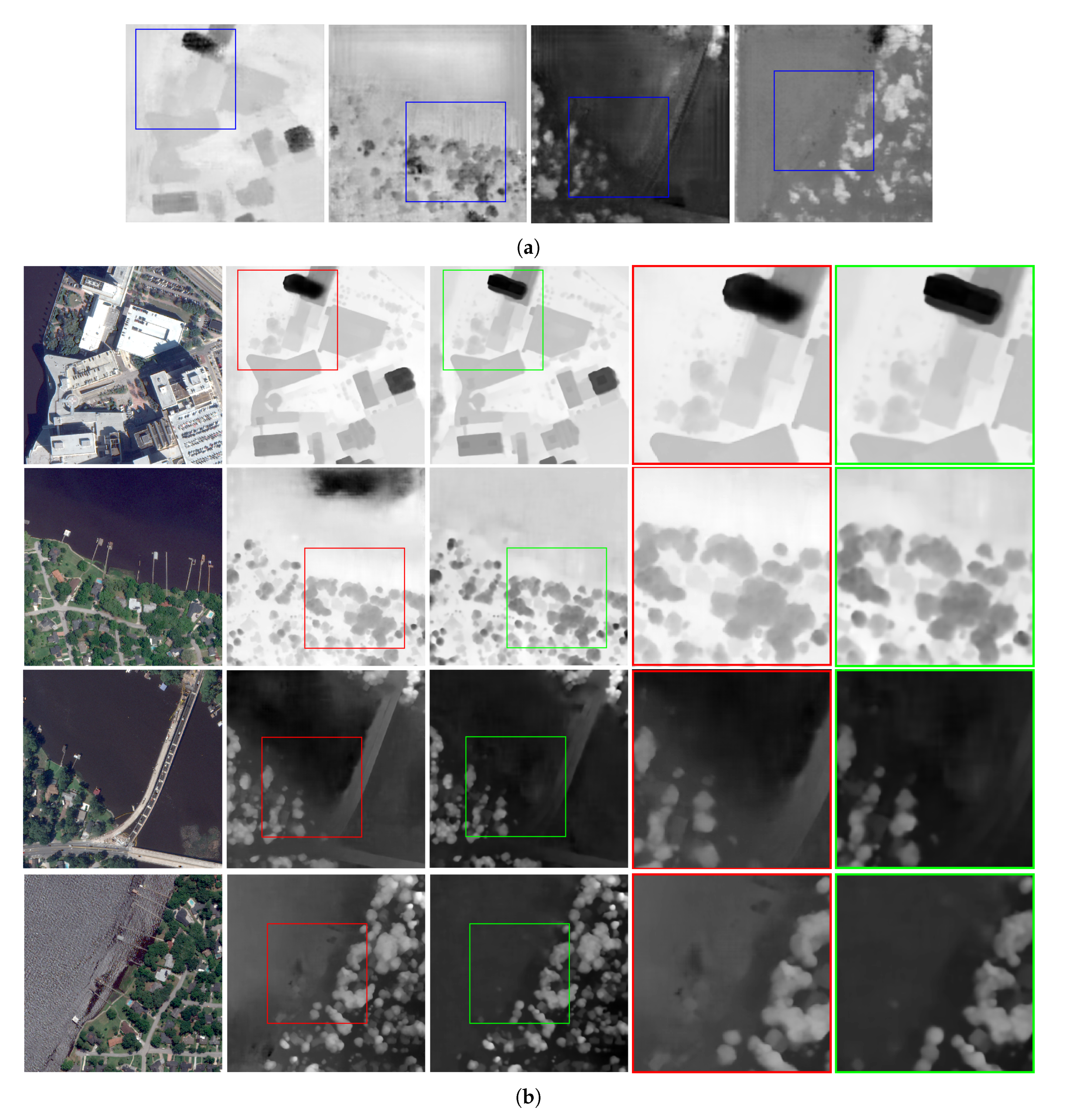
Herein, Figure 7 illustrates the visual performance of disparity estimation in these occluded areas from different algorithms. These scenarios contain various landscapes such as skyscrapers, residential buildings, and woods. The results of DenseMapNet are poor where the pixels of the typical landscapes are almost mismatched (as shown in Figure 7a). However, it is obvious that the results of PSMNet and Bidir-EPNet gain better performance. Hence, we illustrate the details of disparity estimation of our Bidir-EPNet compared to PSMNet in Figure 7b.
First, with the reconstruction of cost volume and disparity regression range, the networks are able to estimate both positive and negative disparities, which lay a foundation for generating bidirectional occlusion-aware maps. Moreover, note that significant improvements compared to PSMNet, such as the disparity precision and fine building structures, can be found from the outlines of buildings. It is remarkable that the bidirectional data loss has eliminated the effect of deformation in occluded areas. The disparity results in the proposed network in occluded areas caused by high buildings show a smooth transition, which also demonstrates the effectiveness of the bidirectional unsupervised loss and the edge-sense second-order smoothness loss.
Moreover, aiming at assessing the generalization of Bidir-EPNet, we choose another six different scenes in OMA test dataset. They contain more complicated landscapes including dense urban areas, a large stadium, expressways, and large forest areas. First, Table 4 shows the two quantitative metrics EPE and D1 of Bidir-EPNet compared with DenseMapNet and PSMNet. It is obvious that Bidir-EPNet performs the best generalization from more complicated areas.
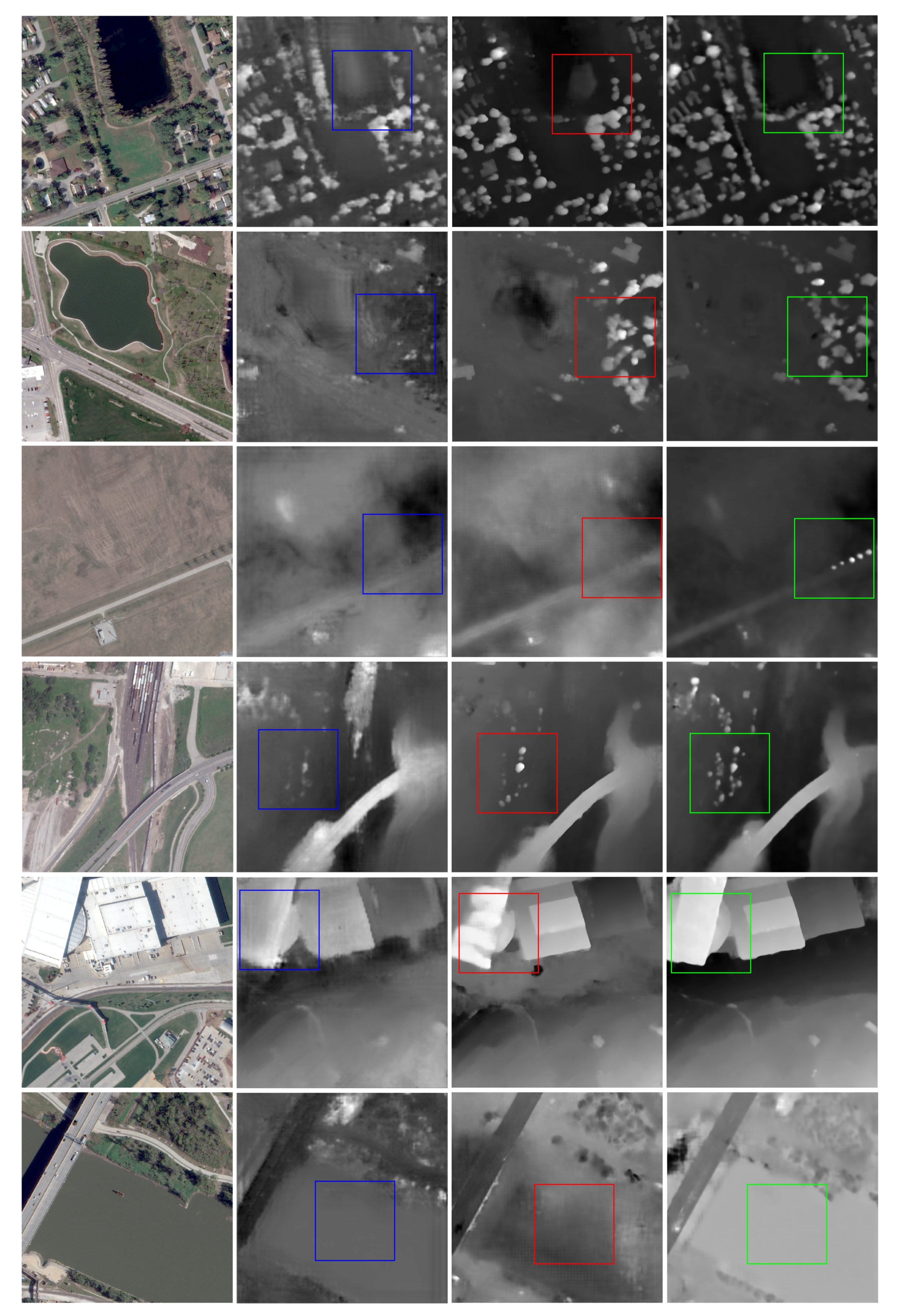
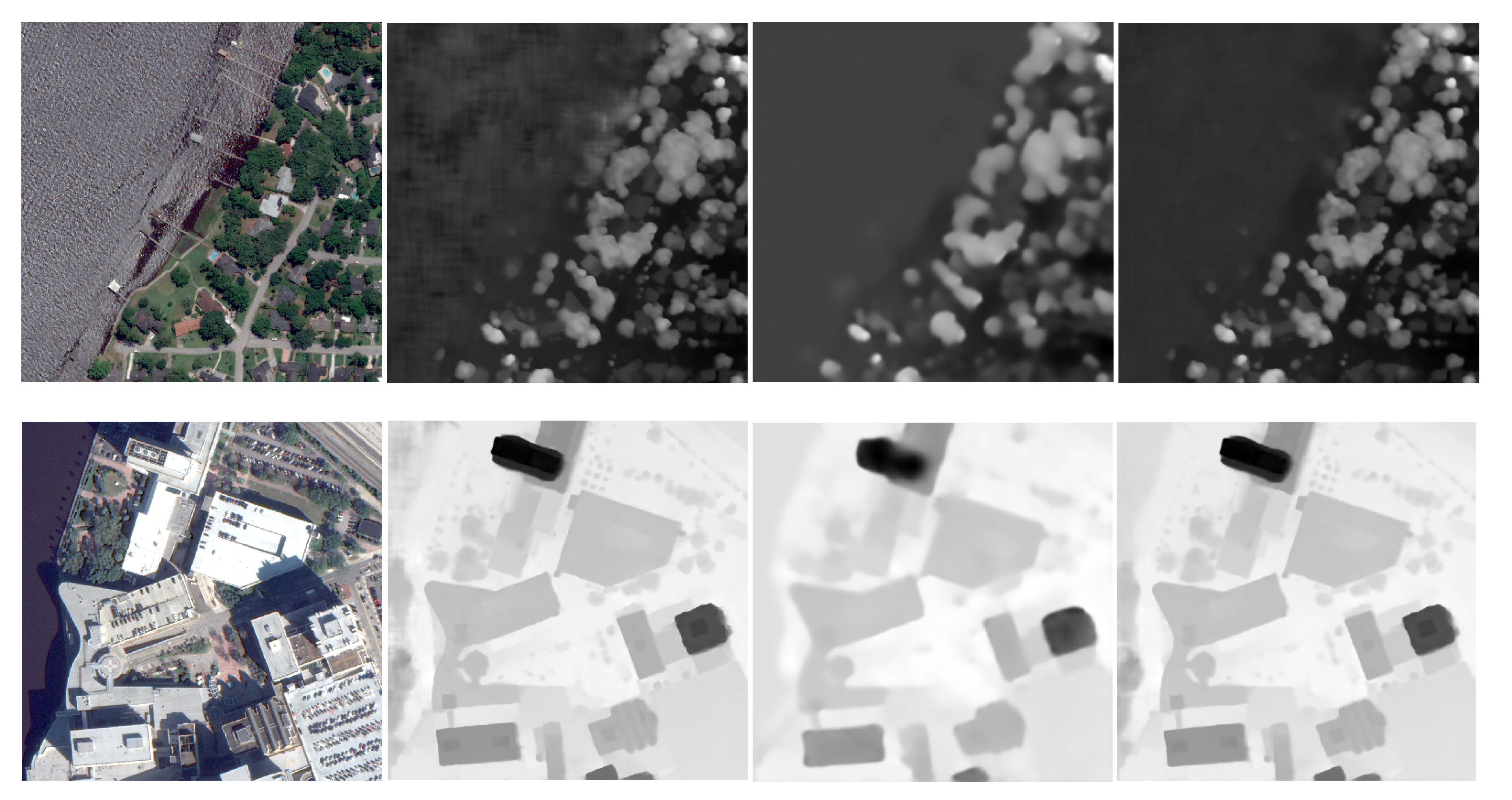
As Figure 8 illustrates, the visual performance of disparity estimation in these scenarios from Bidir-EPNet gains the most satisfying results. From the visual results of the first two scenes, which contain dense areas of urban buildings or woods, DenseMapNet and PSMNet suffer from the confusion between dense houses and woods, while Bidir-EPNet can estimate more accurate building structures and distinguish woods more clearly. That is because the proposed loss functions can eliminate the mutual deformation between these areas. Then, referring to the performance of areas including the expressway (as shown in the third and fourth scenarios in Figure 8), Bidir-EPNet can catch details of the suburban landscapes. In addition, the disparity estimation results of the stadium illustrates that Bidir-EPNet gains more precise structures in detail compared to the other two networks. In general, Bidir-EPNet can handle more complicated scenarios and perform better generalization.

3.2.2. Results on Textureless Areas

In order to further evaluate the performance of our proposed network on textureless areas, four stereo pairs from the dataset are used in this experiment (as shown in Figure 9). In the same way, Table 5 lists the quantitative results (EPE and D1) of different algorithms. Obviously, our proposed network outperforms the other two baselines. DenseMapNet gives the worst results while 8% and 13% in terms of EPE and D1, approximately, are raised by our Bidir-EPNet compared to PSMNet. This proves the significant effectiveness of edge-sense smoothness loss and bidirectional loss, which are able to maintain main structures and predict more precise disparity.
Figure 10 shows the visual results of disparity estimation; they contain a large river area and various landscape features such as tall buildings and woods. As the figure shows, the estimation performances in such textureless areas are ambiguous both from DenseMapNet (Figure 10a) and PSMNet. By comparison, our Bidir-EPNet performs the best since combining the bidirectional occlusion-aware loss and edge-sense smoothness loss estimate more continuous disparity and preserve main structures.
Herein, Figure 10b illustrates the details of disparity estimation of the proposed network compared to PSMNet. The first scenario contains river and skyscrapers in the top-left corner. It is clear that PSMNet is confusing with the prediction of rivers and tall buildings while Bidir-EPNet can gain more precise performance and preserve the main structures simultaneously—that is, the effectiveness of the occlusion influence elimination and edge maintenance generated from the bidirectional unsupervised loss and edge-sense smoothness loss, respectively. From the other three scenarios, which all consist of large areas of water, woods, and bridge across the rivers, more precise disparity estimation can be found in the fine edge of woods, and continuous disparity in large area of rivers. In summary, our Bidir-EPNet gives the best results both on the accuracy of the main structures and smoothness of large textureless regions.
In addition, in order to evaluate the generalization of Bidir-EPNet in textureless areas, we choose another six different scenes in the OMA test dataset which include various textureless areas in suburban areas and large areas of lakes and rivers. Table 6 lists the two quantitative metrics EPE and D1 of Bidir-EPNet compared with DenseMapNet and PSMNet. Bidir-EPNet raises more improvements compared to the other two networks in such textureless areas.
As Figure 11 illustrates, it is obvious that Bidir-EPNet gains the most satisfying visual performance of disparity estimation in these complex textureless areas. From the scenes which contain large area of lakes and rivers, Bidir-EPNet is able to predict much more smooth disparity without eliminating the details of landscapes around them. That is why we use the edge-sense smoothness loss to regularize the network. Under the interaction of the two proposed loss functions, Bidir-EPNet can estimate more continuous disparity in textureless suburban (as shown in the second and third scenes of Figure 11) and distinguish some sporadic landscapes. Moreover, referring to the performance of the fifth scene which contains a textureless roof, the more precise edge structure of the tall building with smooth disparity on the roof can be found by Bidir-EPNet compared to the other two networks. In summary, Bidir-EPNet can predict disparities in multitype textureless areas more smoothly and preserve the main structures around them.

4. Discussion

4.1. Analysis of the Parameter Settings

The parameters in the proposed network include α 1 and α 2 in Equation (3), which are used to control the threshold in occlusion map detection, the parameter γ in Equation (6), which is able to control the edge intensity, and λ 1 , λ 2 , and   λ 3 , which are three weights in our final loss function. As for the parameters α 1 and α 2 , we conduct several parameter settings to find the optimal settings for satellite images. Figure 12 illustrates the detected occlusion maps with different parameter settings. In order to detect accurate occluded pixels, we choose α 1 = 0.02 and α 2 = 1.0 as the parameters to generate the threshold in Equation (3).
As for the parameter γ in Equation (6), which controls the edge intensity, we previously tested different γ for the edge (as shown in Figure 13) to extract effective and helpful edge information. With γ = 1.0 , which is equal to no contribution to edge intensity, the results demonstrate that the range of edge intensity is large, which cannot be directly used in the smoothness loss. With the increase of γ , the edge information is more precise. Consequently, γ is set to 20 with the aim to balance the whole range of edge intensity. It is easy to find out that complicated texture and tiny edge structures still exist in remote sensing images. Finally, to further emphasize sharp main structures, we have clipped the edge weight with a threshold.
As for λ 1 , λ 2 , and λ 3 , which are three weights in our final loss function, we conduct several experiments with combinations of λ 1 , λ 2 , and λ 3 between [ 0 , 1 ] in our final loss function to find the optimal weight setting. As presented in Table 7, the weight setting of 1.0 for smooth L 1 , 0.5 for bidirectional unsupervised loss, and 0.8 for the edge-sense smoothness loss yields the best performance.

4.2. Comparison of Different Unsupervised Loss

The experimental results have demonstrated the effectiveness and significant improvements of our proposed network compared to the two baselines. Subsequently, we are interested in the reason for the application of bidirectional unsupervised loss and edge-sense second-order smoothness loss used in our network. Figure 14 illustrates the comparison results of applying different unsupervised loss. In the beginning, aiming at solving the unignorable problems due to the occluded areas caused by different views, the bidirectional unsupervised loss is proposed to predict more precise disparity. Though it achieves significant improvements in occluded areas (as shown in the second column of Figure 14), the performance of large areas of rivers is ambiguous. Then, the global smoothness loss combining bidirectional loss is used to address this problem. It is obvious that both the disparity in large textureless regions and the edge of main structures become more continuous while losing numerous details (as shown in the third column of Figure 14). Note that the global smoothness loss smooths the disparity crossing the sharp main structure edge, and thus the final loss that combines the second-order smoothness loss and the edge previously extracted based on the intensity of original images is proposed to settle the aforementioned difficulties. As shown in the last column in Figure 14, the visual illustration has proved its effectiveness.

5. Conclusions

In this paper, we propose a novel network based on the PSMNet to improve disparity estimation in occluded areas and textureless areas, which are prevalent in multiview VHR satellite images. By designing a bidirectional cost volume and implementing the bidirectional unsupervised loss and edge-sense second-order smoothness loss, the proposed Bidir-EPNet shows a strong ability to estimate precise disparities and handle the occlusions. Experimental results prove the superiority of the proposed Bidir-EPNet compared to the baselines. To make the proposed network work for other datasets without ground truth labels, we will try to train it further in a complete unsupervised way.

Author Contributions

Conceptualization, R.T.; methodology, R.T.; resources, R.T.; supervision, Y.X. and H.Y.; validation, Y.X.; writing—original draft, R.T.; writing—review and editing, Y.X. and H.Y. All authors have read and agreed to the published version of the manuscript.

Funding

This work was supported in part by the Key Research Program of Frontier Sciences, Chinese Academy of Science, under Grant ZDBS-LY-JSC036, and in part by the National Natural Science Foundation of China under Grant 61901439.

Acknowledgments

The authors would like to thank the Johns Hopkins University Applied Physics Laboratory and the IARPA for providing the data used in this study, and the IEEE GRSS Image Analysis and Data Fusion Technical Committee for organizing the Data Fusion Contest.

Conflicts of Interest

The authors declare no conflict of interest.

References

  1. Scharstein, D.; Szeliski, R. A taxonomy and evaluation of dense two-frame stereo correspondence algorithms. Int. J. Comput. Vis. 2002, 47, 7–42. [Google Scholar] [CrossRef]
  2. Hirschmüller, H. Stereo processing by semiglobal matching and mutual information. IEEE Trans. Pattern Anal. Mach. Intell. 2008. [Google Scholar] [CrossRef] [PubMed]
  3. Hermann, S.; Klette, R.; Destefanis, E. Inclusion of a second-order prior into semi-global matching. In Pacific-Rim Symposium on Image and Video Technology; Springer: Berlin/Heidelberg, Germany, 2009; pp. 633–644. [Google Scholar]
  4. Zhu, K.; d’Angelo, P.; Butenuth, M. A performance study on different stereo matching costs using airborne image sequences and satellite images. In Lecture Notes in Computer Science, Proceedings of the ISPRS Conference on Photogrammetric Image Analysis, Munich, Germany, 5–7 October 2011; Springer: Berlin/Heidelberg, Germany, 2011; pp. 159–170. [Google Scholar]
  5. Žbontar, J.; LeCun, Y. Stereo matching by training a convolutional neural network to compare image patches. J. Mach. Learn. Res. 2016, 17, 2287–2318. [Google Scholar]
  6. Luo, W.; Schwing, A.G.; Urtasun, R. Efficient deep learning for stereo matching. In Proceedings of the IEEE Conference on Computer Vision and Pattern Recognition, Las Vegas, NV, USA, 27–30 June 2016; pp. 5695–5703. [Google Scholar]
  7. Guney, F.; Geiger, A. Displets: Resolving stereo ambiguities using object knowledge. In Proceedings of the IEEE Conference on Computer Vision and Pattern Recognition, Boston, MA, USA, 7–12 June 2015; pp. 4165–4175. [Google Scholar]
  8. Seki, A.; Pollefeys, M. Sgm-nets: Semi-global matching with neural networks. In Proceedings of the IEEE Conference on Computer Vision and Pattern Recognition, Honolulu, HI, USA, 21–26 July 2017; pp. 231–240. [Google Scholar]
  9. Mayer, N.; Ilg, E.; Hausser, P.; Fischer, P.; Cremers, D.; Dosovitskiy, A.; Brox, T. A large dataset to train convolutional networks for disparity, optical flow, and scene flow estimation. In Proceedings of the IEEE Conference on Computer Vision and Pattern Recognition, Las Vegas, NV, USA, 27–30 June 2016; pp. 4040–4048. [Google Scholar]
  10. Pang, J.; Sun, W.; Ren, J.S.; Yang, C.; Yan, Q. Cascade residual learning: A two-stage convolutional neural network for stereo matching. In Proceedings of the IEEE International Conference on Computer Vision Workshops, Venice, Italy, 22–29 October 2017; pp. 887–895. [Google Scholar]
  11. Kendall, A.; Martirosyan, H.; Dasgupta, S.; Henry, P. End-to-End Learning of Geometry and Context for Deep Stereo Regression. In Proceedings of the IEEE International Conference on Computer Vision (ICCV), Venice, Italy, 22–29 October 2017; pp. 66–75. [Google Scholar]
  12. Chang, J.; Chen, Y. Pyramid Stereo Matching Network. In Proceedings of the 2018 IEEE Conference on Computer Vision and Pattern Recognition, Salt Lake City, UT, USA, 18–22 June 2018; pp. 5410–5418. [Google Scholar] [CrossRef] [Green Version]
  13. Sundaram, N.; Brox, T.; Keutzer, K. Dense Point Trajectories by GPU-Accelerated Large Displacement Optical Flow; ECCV; Springer: Berlin/Heidelberg, Germany, 2010; pp. 438–451. [Google Scholar]
  14. Xiang, Y.; Wang, F.; Wan, L.; Jiao, N.; You, H. Os-flow: A robust algorithm for dense optical and sar image registration. IEEE Trans. Geosci. Remote Sens. 2019, 57, 6335–6354. [Google Scholar] [CrossRef]
  15. Meister, S.; Hur, J.; Roth, S. UnFlow: Unsupervised learning of optical flow with a bidirectional census loss. In Proceedings of the 32nd AAAI Conference on Artificial Intelligence, New Orleans, LA, USA, 2–7 February 2018; pp. 7251–7259. [Google Scholar]
  16. Girshick, R. Fast r-cnn. In Proceedings of the IEEE International Conference on Computer Vision, Santiago, Chile, 7–13 December 2015; pp. 1440–1448. [Google Scholar]
  17. Sun, D.; Roth, S.; Black, M. A quantitative analysis of current practices in optical flow estimation and the principles behind them. Int. J. Comput. Vis. 2014. [Google Scholar] [CrossRef] [Green Version]
  18. Trobin, W.; Pock, T.; Cremers, D.; Bischof, H. An unbiased second-order prior for high-accuracy motion estimation. In Joint Pattern Recognition Symposium; Springer: Berlin/Heidelberg, Germany, 2008; pp. 396–405. [Google Scholar]
  19. Zhang, C.; Li, Z.; Cai, R.; Chao, H.; Rui, Y. As-rigid-as-possible stereo under second order smoothness priors. In European Conference on Computer Vision; Springer: Berlin/Heidelberg, Germany, 2014; pp. 112–126. [Google Scholar]
  20. Bosch, M.; Foster, K.; Christie, G.; Wang, S.; Hager, G.D.; Brown, M. Semantic Stereo for Incidental Satellite Images. In Proceedings of the 2019 IEEE Winter Conference on Applications of Computer Vision, Waikoloa Village, HI, USA, 7–11 January 2019; pp. 1524–1532. [Google Scholar] [CrossRef] [Green Version]
  21. Le Saux, B.; Yokoya, N.; Hansch, R.; Brown, M.; Hager, G. 2019 Data Fusion Contest [Technical Committees]. IEEE Geosci. Remote Sens. Mag. 2019, 7, 103–105. [Google Scholar] [CrossRef]
  22. Atienza, R. Fast Disparity Estimation Using Dense Networks. In Proceedings of the IEEE International Conference on Robotics and Automation, Brisbane, Australia, 21–25 May 2018; pp. 3207–3212. [Google Scholar] [CrossRef] [Green Version]
Figure 1. The variety of disparities in remote sensing stereo pairs of the US3D dataset.
Remotesensing 12 04025 g001
Figure 2. The architecture of the proposed edge-sense bidirectional pyramid network: the input stereo pairs are concatenated by the normal and reverse pairs. As the network is trained, the forward and backward occlusion-aware maps are generated to reduce the deformation by masking the occluded pixel, and the structure information is extracted from the input pairs, acting as an edge-sense prior for second-order smoothness loss.
Remotesensing 12 04025 g002
Figure 3. Reconstruction of the cost volume with the stacked feature maps, which has the size of [ 2 × F × H × W ] , covering disparities that range from D m a x to D m a x , where F denotes the number of feature maps and H and W are the height and width of the input images, respectively.
Remotesensing 12 04025 g003
Figure 4. Bidirectional disparity maps. (a) The left image. (b) The disparity map based on the left image. (c) The right image. (d) The disparity map based on the right image.
Remotesensing 12 04025 g004
Figure 5. Bidirectional occlusion-aware maps.
Remotesensing 12 04025 g005
Figure 6. The examples of left images that contain occluded regions, the tile numbers of these images (from left to right) are: JAX-068-014-013, JAX-168-022-005, JAX-260-022-001, OMA-288-036-038, OMA-212-038-033.
Remotesensing 12 04025 g006
Figure 7. The comparison of different networks. Results in (a) are generated from DenseMapNet while (b) illustrates the results from PSMNet and Bidir-EPNet in detail. The columns from left to right represent Left image, PSMNet, Bidir-EPNet, ROI of PSMNet, and ROI of Bidir-EPNet, respectively.
Remotesensing 12 04025 g007
Figure 8. The generalization of different networks. The columns from left to right represent Left image, DenseMapNet, PSMNet, and Bidir-EPNet, respectively.
Remotesensing 12 04025 g008
Figure 9. The examples of left images that contain textureless regions, the tile numbers of these images (from left to right) are: JAX-214-011-004, JAX-269-013-025, JAX-236-002-001, JAX-269-018-013.
Remotesensing 12 04025 g009
Figure 10. The comparison of different networks results in (a) are generated from DenseMapNet, whereas (b) illustrates the results from PSMNet and Bidir-EPNet in detail. The columns from left to right represent Left image, PSMNet, Bidir-EPNet, ROI of PSMNet, and ROI of Bidir-EPNet, respectively.
Remotesensing 12 04025 g010
Figure 11. The generalization of different networks. The columns from left to right represent Left image, DenseMapNet, PSMNet, and Bidir-EPNet, respectively.
Remotesensing 12 04025 g011
Figure 12. Different settings for parameters α 1 and α 2 .
Remotesensing 12 04025 g012
Figure 13. From left to right: Left image, weight maps of smooth term with γ = 1.0 , γ = 20.0 , and γ = 20.0 with a threshold of 0.3.
Remotesensing 12 04025 g013
Figure 14. The comparison of different loss function. The columns from left to right denote: Left images, only bidirectional unsupervised loss, bidirectional, and smoothness loss without edge previously, the final loss.
Remotesensing 12 04025 g014
Table 1. The datasets configurations for experiments: JAX represents Jacksonville and OMA denotes Omaha.
Stereo PairModePatch SizeNumber of Images: Training/TestingUsage
JAXRGB 1024 × 1024 1500/346Training and Testing
OMARGB 1024 × 1024 –/2086Testing
Table 2. The comparison of averaged endpoint error (EPE) (pixel) and fraction of erroneous pixels (D1) (%). The best results are labeled as bold.
NetworksJAXOMA
EPED1EPED1
DenseMapNet1.865715.341.625114.84
PSMNet1.36449.511.51229.15
Bidir-EPNet1.27648.031.48998.96
Table 3. The comparison of EPE and D1 of occluded regions. The best results are labeled as bold.
Tile NumberDenseMapNetPSMNetBidir-EPNet
EPED1EPED1EPED1
JAX-068-014-0133.5932.11.319.201.147.49
JAX-168-022-0051.409.880.893.540.803.27
JAX-260-022-0012.4020.60.944.160.913.55
OMA-288-036-0381.4010.00.914.540.884.37
OMA-212-038-0331.329.541.227.140.983.78
Table 4. The comparison of EPE and D1 of occluded regions in OMA. The best results are labeled as bold.
Tile NumberDenseMapNetPSMNetBidir-EPNet
EPED1EPED1EPED1
OMA-276-040-0382.7231.63.1133.61.8417.3
OMA-172-041-0361.6914.61.6210.91.207.03
OMA-225-031-0273.0737.34.3341.21.4810.3
OMA-247-034-0381.498.472.059.120.712.14
OMA-248-036-0272.2317.91.609.670.963.65
OMA-203-041-0381.8518.11.6410.01.296.41
Table 5. The comparison of EPE and D1 of textureless regions. The best results are labeled as bold.
Tile NumberDenseMapNetPSMNetBidir-EPNet
EPED1EPED1EPED1
JAX-214-011-0042.2723.311.135.811.044.72
JAX-269-013-0251.6715.761.015.960.924.68
JAX-236-002-0011.3211.181.027.330.986.52
JAX-269-018-0132.6929.271.6313.711.4511.12
Table 6. The comparison of EPE and D1 of occluded regions in OMA. The best results are labeled as bold.
Tile NumberDenseMapNetPSMNetBidir-EPNet
EPED1EPED1EPED1
OMA-134-004-0081.7215.91.6714.71.229.27
OMA-176-031-0261.3410.20.966.900.856.86
OMA-181-027-0280.911.450.981.480.861.35
OMA-211-033-0312.0918.11.316.101.114.32
OMA-251-043-0416.6645.14.2923.51.928.74
OMA-292-039-0031.073.581.763.381.382.93
Table 7. The comparison of EPE (pixel) with different loss weights. The best result is labeled as bold.
Loss WeightEPE(Pixel)
λ 1 λ 2 λ 3
1.00.00.01.36
1.00.10.31.33
1.00.30.51.30
1.00.50.81.27
1.00.80.91.29
1.01.01.01.29
Publisher’s Note: MDPI stays neutral with regard to jurisdictional claims in published maps and institutional affiliations.