Article

Evaluation of Precipitation Products by Using Multiple Hydrological Models over the Upper Yellow River Basin, China

1
College of Hydrology and Water Resources, Hohai University, Nanjing 210098, China
2
Research Center for Climate Change, Ministry of Water Resources, Nanjing 210029, China
3
State Key Laboratory of Hydrology-Water Resources and Hydraulic Engineering, Nanjing Hydraulic Research Institute, Nanjing 210029, China
4
School of Resources and Environment, University of Electronic Science and Technology of China, Chengdu 611731, China
*
Author to whom correspondence should be addressed.
Remote Sens. 2020, 12(24), 4023; https://doi.org/10.3390/rs12244023
Submission received: 13 November 2020 / Revised: 5 December 2020 / Accepted: 6 December 2020 / Published: 9 December 2020

Abstract

:
In this study, 6 widely used precipitation products APHRODITE, CPC_UNI_PRCP, CN05.1, PERSIANN-CDR, Princeton Global Forcing (PGF), and TRMM 3B42 V7 (TMPA), were evaluated against gauge observations (CMA data) from 1998 to 2014, and applied to streamflow simulation over the Upper Yellow River basin (UYRB), using 4 hydrological models (DWBM, RCCC-WBM, GR4J, and VIC). The relative membership degree (u), as the comprehensive evaluation index in the hydrological evaluation, was calculated by the optimum fuzzy model. The results showed that the spatial pattern of precipitation from the CMA dataset and the other 6 precipitation products were very consistent with each other. The satellite-derived rainfall products (SDFE), like PSERSIANN-CDR and TMPA, depicted considerably finer and more detailed spatial heterogeneity. The SDFE and reanalysis (RA) products could estimate the monthly precipitation very well at both gauge and basin-average scales. The runoff simulation results indicated that the APHRODITE and TMPA were superior to the other 4 precipitation datasets, obtaining much higher scores, with average u values of 0.88 and 0.77. The precipitation estimation products tended to show better performance in streamflow simulation at the downstream hydrometric stations. In terms of performance of hydrological models, the RCCC–WBM model showed the best potential for monthly streamflow simulation, followed by the DWBM. It indicated that the monthly models were more flexible than daily conceptual or distributed models in hydrological evaluation of SDFE or RA products, and that the difference in precipitation estimates from various precipitation datasets were more influential in the GR4J and VIC models.

Graphical Abstract

1. Introduction

Hydrological models are the most important and efficient tools developed over the past decades to quantify each terrestrial and meteorological component of the water cycle, for past, present, and future conditions [1,2,3]. Worldwide, they facilitate the efficient knowledge and management of water cycles and resources, such as supporting flood warnings, estimating drinking water availability, determining ecological flows required to maintain a healthy environment, and optimizing water allocation schemes.
Precipitation, an important part of the water cycle, plays an influential role in the quantitative description of hydrological processes and regional water balance. Furthermore, as the most crucial atmospheric forcing for hydrological modelling, the accuracy, and spatio-temporal resolution of precipitation data influence the accuracy of the models’ applications to a large extent. However, the comprehensive and efficient acquisition of precipitation observations, takes a lot of time and money, especially in cold and sparsely populated high-altitude areas, which are often the source of some important big rivers and where the collection of basic hydrometeorological information is essential. The Upper Yellow River Basin (UYRB) is one such area, located in the northeast Qinghai–Tibet Plateau, with a mean altitude of approximately 4000 m above sea level. Known as the “water tower” of the Yellow River, the UYRB occupies an area of 0.122 million km2, about 15% of the total area, but contributes approximately 35% of the total annual runoff recorded at the Lijin hydrometric station, downstream of the Yellow River [4]. However, there are only 9 basic national meteorological observation stations (managed by Chinese Meteorology Administration, CMA) over the whole UYRB, with a density of 1 station per 1° × 1° grid. The spatial distribution of the meteorological stations is also highly uneven and most stations are located around the river channels with a relatively low elevation. Therefore, streamflow simulation using the limited gauge-based precipitation information might not be reliable due to the input uncertainties, with such a poor spatial resolution. In this context, researchers are considering the use of satellite-derived rainfall estimates (SDFE) or reanalysis precipitation (RA) products as an alternative [5,6]. These estimates have suitable spatio-temporal resolution (e.g., 0.25° and 24 h), released uninterrupted and in near real-time, publicly available and easily accessible, and hold great potential as forcing data for streamflow modelling, and projection in data-sparse and ungauged basins [7].
However, the SDFE are also subject to a variety of potential errors and uncertainties [8], such as gaps in revisit times [9], a weak direct relationship between remotely sensed signals and precipitation rate [10], and atmospheric effects that modify the radiation field and the different climatic zones with different radiation albedo. For the reanalysis precipitation products, uncertainties and errors mainly stem from the data sources, the interpolation algorithm, and the data assimilation system [6,11]. Therefore, the applicability and precision are required through validation before wide application. Normally, there are 2 types of validation efforts of SDFE or RA products—(1) directly comparing the SDFE or RA products estimates against the precipitation gauge data [12,13,14]; and (2) evaluation of the precipitation estimates based on their predictive ability of streamflow in a hydrological modeling framework [5,15]. For example, Zhang et al. [16] evaluated three precipitation products—GLDAS (global land data assimilation system), TMPA (the TRMM Multi-satellite Precipitation Analysis, TMPA 3B42V7), and ERA-Interim (European Centre for Medium-Range Weather Forecasts, ECMWF), together with three interpolation methods (the inverse distance-weighted method, the bilinear interpolation method, and the nearest point method) based on the SWAT (Soil and Water Assessment Tool) model in the Hun River basin, in Northeast China. They found that hydrological simulations forced by the APHRODITE dataset were the best in capturing daily and monthly measured streamflow. Moreover, the bilinear interpolation was more appropriate to interpolate the grid precipitation to rain gauge. Poméon et al. [5] evaluated the performance of remotely sensed and reanalysis precipitation data over six differently sized and located basins in West Africa, by using the HBV light model. The results showed that while performances differ, most datasets manage to somewhat accurately predict the observed streamflow in a given basin. Best results were achieved by datasets that use a multitude of input data, namely infrared and microwave satellite data, as well as observations from rain gauges for bias correction. Over the UYRB, Meng et al. [15] tested the suitability of TRMM satellite precipitation for daily and monthly hydrological process simulation, by using the SWAT model. Su et al. [17] evaluated the applicability of four latest satellite-gauge combined precipitation estimates (CMORPH CRT and BLT, PERSIANN-CDR, and TRMM 3B42 Version 7) for extreme precipitation and streamflow predictions in the UYRB, based on the Variable Infiltration Capacity (VIC) model, and suggested that four satellite-gauge combined precipitation datasets could generally capture the spatial distribution of precipitation well and should be used with caution in simulating massive flood events. Yuan et al. [18] applied the TMPA 3B42V7 satellite precipitation and IMERG Final run V05 products in daily streamflow and flood events (sub-daily scale) simulation, by using the grid-based Xinanjiang (GXAJ) model and proposed that the low correlation coefficients values between the estimated precipitation against the station measurements, existed in both the IMERG and 3B42V7 products, in particular, at a sub-daily temporal scale. They also found that the GXAJ model’s parameters needed to be well-regulated to fit the simulated flood events from different precipitation forcing datasets to the observed processes.
Although a lot of research about the suitability of SDFE or RA datasets in regional water balance modeling was conducted, there are still many factors that can influence the performance of SDFE or RA precipitation products in hydrological modeling, in addition to errors in precipitation estimation. These factors include interpolation algorithm [16], data series length [9], and the choice of evaluation metrics and model calibration method. Uncertainties might also be introduced into an analysis by the choice of the hydrological models. In particular, optimizing parameters, governing infiltration and evaporation in streamflow simulation, might weaken the effects of precipitation over- or underestimation [5]. Gudmundsson et al. [19] applied 9 hydrological models in large-scale modeling in Europe with the same atmospheric forcing data, and suggested that any single model should be applied with caution as there is a great risk of biased conclusions, leading to a large spread in model performance.
Given these advantages and shortcomings, this study (1) used multiple performance indicators to evaluate the performance of multiple SDFE and RA precipitation products in precipitation estimation, at both station and basin average scale, based on the multi-objective optimum fuzzy evaluation model. (2) Then, the capacity of streamflow modeling of precipitation products was evaluated by using three conceptual hydrological models with significantly different structures and a physically grid-based distributed hydrological model (VIC). (3) Furthermore, the influence of model structure on streamflow reproduction capacity based on a variety of precipitation products were well-studied and discussed. (4) The suggestions about the selection of precipitation products and hydrological models in different hydrological research and applications is given at last.

2. Study Area

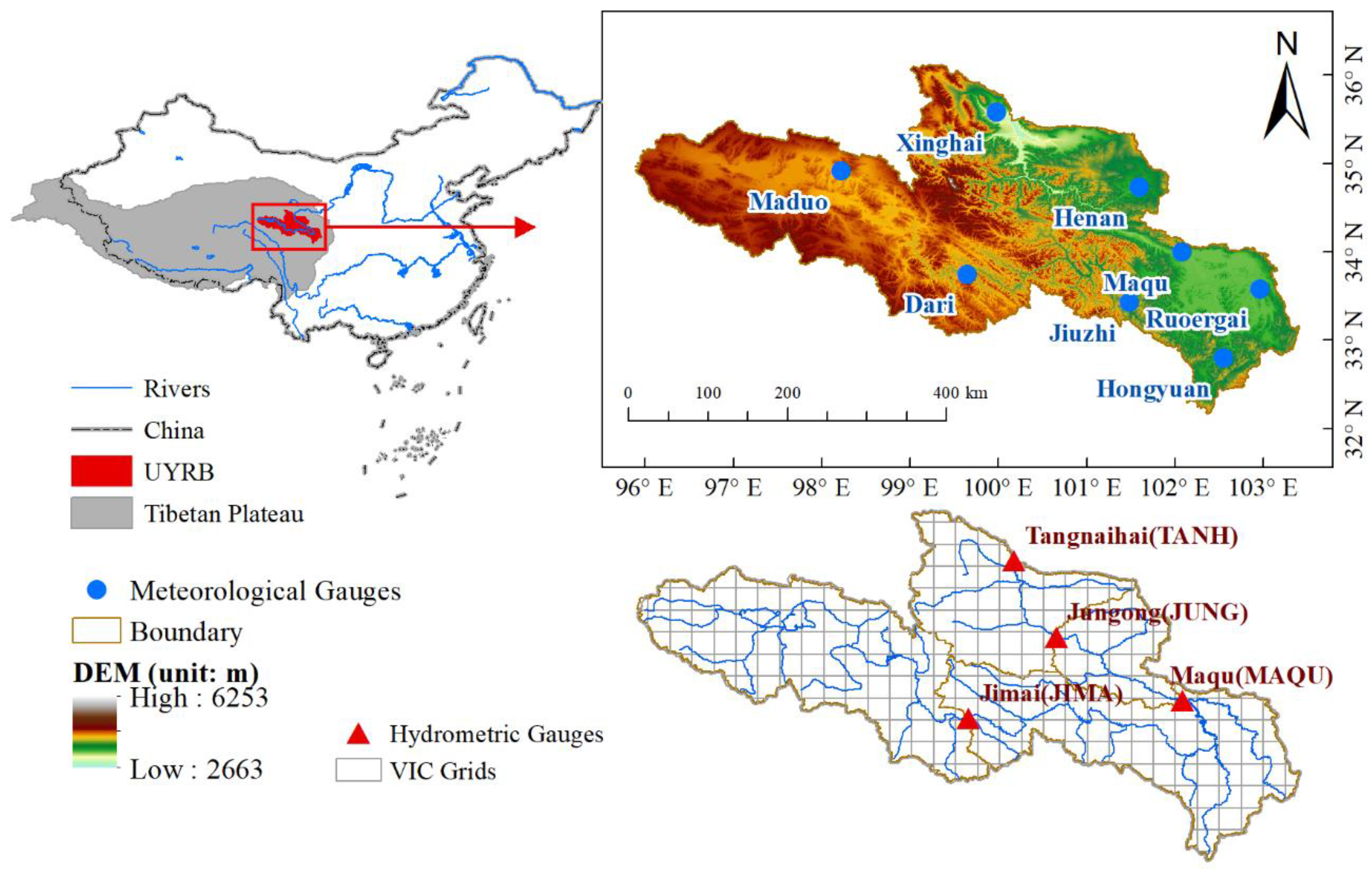
The UYRB is located in the Eastern Qinghai–Tibet Plateau, China. The geographical location is between 32.17°–36°N, 95.8°–103.5°E, the area controlled by the Tangnaihai (TANH) hydrological station, as shown in Figure 1. The topography and landforms in the basin are complex, with diverse geomorphic units including alpine valleys in the lower reaches, grasslands, lakes, and marshes, in the middle reaches, and sparse grasslands in the upper reaches [17]. The average elevation of the basin is about 3000 m, and the source area is as high as 4400 m. The terrain is high in the west and comparatively low in the east, partially maintaining the characteristics of the surrounding high and low basins. The main basin boundary lines are the Bayan Har Mountains in the northwest-southeast direction and the Buqing Mountain in the northwest. Sandy loam, sandy clay, and loamy sand are the main soil types. The region has typical continental plateau climate characteristics. The mean annual temperature decreases from east to west as the altitude increases. The basin-average mean annual precipitation is approximately 484.2 mm, and the precipitation mainly comes from the Indian Ocean water vapor, brought by the warm and humid air current in the Bay of Bengal. Precipitation is mainly concentrated in the months of June to September, accounting for 75% to 90% of the whole year. The precipitation is mostly in the form of snowfall in dry season and heavy rain in wet season, with good water and heat condition in the same season. The snow cover period in most areas of the UYRB is generally from November to the end of April of the following year [18]. Yuan et al. [18] suggested that the UYRB is subject to minimal human activities and can be regarded as a relatively pristine area, because neither large irrigation projects nor reservoirs exist in this area. Taking into account the representativeness of different regions, four hydrometric stations over the UYRB were selected to evaluate the applicability of different precipitation products, as shown in Table 1.

3. Data and Method

3.1. SDFE and RA Precipitation Products

The recorded precipitation data obtained from the China Surface Climate Daily Data Set V3.0 (CMA) was used to test the precision and applicability of the multiple precipitation estimates dataset, at point scale. The CMA data, provided by the National Meteorological Information Center of China (http://data.cma.cn/), covers air pressure (daily average, maximum, and minimum), air temperature, precipitation, evaporation, relative humidity, wind direction and speed, sunshine hours, and ground surface temperature, at 699 national standard meteorological gauges in China, in line with standard quality control methodology. Due to the high quality of the meteorological data, missing data can be ignored. The 8 standard gauges in the UYRB are shown in Figure 1.
Table 2 lists the main information about the SDFE or RE datasets used in this study, including APHRODITE, CN05.1, Climate Prediction Center Unified Gauge-Based Analysis of Global Daily Precipitation (CPC_UNI_PRCP), Precipitation Estimation from Remotely Sensed Information using Artificial Neural Networks-Climate Data Record (PERSIANN-CDR), Princeton global forcing (PGF) dataset, and TRMM Multi-satellite Precipitation Analysis (TMPA) precipitation product. The brief description (such as data sources and temporal and spatial resolution) were as follows.

3.1.1. APHRODITE

The APHRODITE dataset, developed by the research foundation of the Japan Meteorological Agency (JMA) [20], is based on rain gauge-based daily precipitation data from 5000–12,000 valid stations, the GTS-based dataset from the World Meteorological Organization (WMO) and the National Data Center (NCDC)/National Oceanic and Atmospheric Administration (NOAA), and monthly precipitation data for Iran, Thailand, Israel, and Turkey [26]. For Central Asia, precipitation reanalysis data were produced with 0.25° × 0.25° spatial resolution for the period 1951–2007 (V1101). In 2018, the extension updates for the period of 2008–2015 (V1101EX_R1) were released for diagnosing climate variability and related hydrological studies, and created with the same algorithm (V1101). Further explanation can be found at http://aphrodite.st.hirosaki-u.ac.jp.

3.1.2. CN05.1

The CN05.1 dataset is provided by the National Meteorological Information Center of China (https://www.ncc-cma.net). As discussed by Xu et al. [27], the CN05.1 dataset was constructed by the “anomaly approach” during the interpolation, but with more station observations (~2400 basic, benchmark and general stations) in China [22]. In the “anomaly approach”, a gridded climatology was first calculated, and then a gridded daily anomaly was added to the climatology, to obtain the final dataset.

3.1.3. CPC_UNI_PRCP

The Climate Prediction Center Unified Gauge-Based Analysis of Global Daily Precipitation (CPC_UNI_PRCP) was the first product of the CPC Unified Precipitation Project underway at the NOAA Climate Prediction Center (http://www.cpc.ncep.noaa.gov). The primary goal of the project was to create a suite of unified precipitation products of consistent quantity and improved quality, by combining all information sources available at the CPC and by taking advantage of the optimal interpolation (OI) objective analysis technique. The dataset included gauge-based daily precipitation data for global land areas, with a resolution of 0.5° on a regular latitude–longitude grid [21].

3.1.4. PERSIANN-CDR

The PERSIANN-CDR (Precipitation Estimation from Remotely Sensed Information using Artificial Neural Networks—Climate Data Record) is a near-global 30+ year high-resolution precipitation dataset for long-term studies and was developed by the Center for Hydrometeorology and Remote Sensing (CHRS) at the University of California, Irvine (UCI, http://chrsdata.eng.uci.edu) [28]. It was designed to address the need for a consistent, long-term, high-resolution, and global precipitation dataset for studying the changes and trends in daily precipitation, especially extreme precipitation events due to climate change and natural variability. The PERSIANN-CDR was generated from the PERSIANN algorithm, using the GridSat-B1 infrared data and adjusted using the Global Precipitation Climatology Project (GPCP) monthly product, to maintain consistency of the two datasets at a 2.5-degree monthly scale, throughout the entire record.

3.1.5. PGF

The Princeton global forcing (PGF) dataset provides near-surface meteorological data for driving land surface models and other terrestrial modeling systems [24]. It was constructed by combining a suite of global observation-based datasets with the NCEP/NCAR reanalysis. The dataset was available (http://hydrology.princeton.edu/data.php) at 1.0-degree (plus 0.5 and 0.25 degree), 3-hourly (plus daily and monthly) resolution globally for 1948–2016.

3.1.6. TMPA

The TRMM Multi-satellite Precipitation Analysis (TMPA) is based on the calibration by the TRMM Combined Instrument (TCI) and TRMM Microwave Imager (TMI) precipitation products, respectively [25]. The description of the dataset parallels that of Reference [18]. In this study, we used the latest version of the TMPA V7 research product (3B42). This daily accumulated precipitation product was generated from the research-quality 3-hourly TRMM Multi-Satellite Precipitation Analysis TMPA (3B42). It was produced at the NASA GES DISC, as a value-added product, which is available from January 1998 till present and accessible at https://disc.gsfc.nasa.gov/datasets/TRMM_3B42_Daily_7.

3.2. Hydrological Models

3.2.1. DWMB

The DWMB monthly water balance model developed by Deng et al. [29], is based on the optimality principle of entropy or power or the generalized proportionality relationship [30]. This model is a modification of the “abcd” model developed by Thomas and Harold [31]. Both the “abcd” model and the SCS curve number method use Budyko-type functions to simulate surface runoff at the event scale. This monthly water balance model divides the available water (sum of previous soil moisture and precipitation) into three components—underground water storage, evapotranspiration, and runoff—using two parameters in a unified form of a Byduko-type function. To take into account the effect of snow storage and melt, a simple temperature-based module was added to the DWBM. The total precipitation was partitioned into rain and snow, based on two critical temperature values and the accumulated snow storage was an infinite capacity tank, where the snowmelt was released at a rate determined by the mean daily minimum temperature and the snowmelt coefficient, and then added to the available water. The model’s functions and its parameters are detailed in Reference [30].

3.2.2. RCCC-WBM

The RCCC-WBM model is a simplified large-scale conceptual hydrological model [32], which was widely used to model the monthly streamflow process and water resources at the catchment scale. The runoff simulated by RCCC-WBM model contains three components—surface flow, snowmelt-driven flow, and baseflow. In this model, monthly precipitation is divided into rainfall and snowfall with the upper and lower temperature criteria, using the linear partitioning method. The model calculation flowchart and formula are detailed in Guan et al. [33]. Normally, in previous studies, the upper and lower temperatures were preset as 4 °C and −4 °C without calibration in flow simulation. However, in the UYRB, the monthly average minimum temperatures were normally below 3 °C and less than −15 °C in winter (December, January, and February) and −3 °C in spring (March, April, and May). In this study, the values of upper and lower temperatures were also calibrated for each hydrometric station. The RCCC-WBM model had only four parameters, excluding the solid–liquid precipitation partition model (e.g., upper and lower temperature criteria value), and was successfully applied in semi-arid and humid catchments located in China [34]. It is characterized by a simple structure, fewer parameters, and flexibility in utility. Refer to Table 3 for more information about the parameters.

3.2.3. GR4J

The GR4J model, developed by the research group at the CEMAGREF (now IRSTEA) [35], is an empirical and parsimonious, reservoir-based model. The description of the model parallels that of Guan et al. [33]. Initially, this model had only 4 parameters (shown in Table 3), and most secondary processes are represented by empirical constants, which was widely used in Europe and Australia [36,37]. The model calculates effective rainfall by first deducting evaporation and interception from gauged precipitation. Then, part of the effective rainfall goes into the runoff production store and the rest is divided into two parts, 90% of which infiltrates into the routing store and forms the slow flow with a unit hydrograph, while the remaining 10% forms the fast flow. As for the snowmelt simulation, the snowfall-snowmelt processes of the Soil and Water Assessment Tool (SWAT, Neitsch et al. [38]) were incorporated into the GR4J. Daily snowmelt is utilized in the rainfall-runoff processes, including interception, soil moisture, ground water, and runoff generation. The descriptions of the rainfall-snowfall separation, snowfall accumulation, and snowmelt functions are detailed in Neitsch et al. [38] and Li et al. [39].

3.2.4. VIC

The Variable Infiltration Capacity (VIC) model, developed by Liang et al. [40], is well-known as a macroscale and semi-distributed land surface hydrological model in simulating the water and energy fluxes that govern the terrestrial hydrological cycle, over a grid mesh. Lohmann et al. [41] introduced a flow routing model that traces the river channel flow triggered by the runoff from the individual grid cells, which facilitated the distributed application of the VIC for rainfall-runoff processes at large domains. In order to extend the model to different climate zones or apply the model globally, various updates for specific fields were issued, including physically based frozen soil algorithm updates, cold land process modification, snow blowing model, and lake and wetland updates. More details of the model are provided at the official website (https://vic.readthedocs.io/en/master/). Fortunately, Wi et al. [42] developed a user-friendly software package, the VIC-Automated Setup Toolkit (VIC-ASSIST), accessible through an intuitive MATLAB graphical user interface. The source code of this tool is archived in Git and is publicly available through GitHub: https://github.com/sungwookwi/VIC-ASSIST. The automated processes of this tool include watershed delineation, climate and geographical input set-up, model parameter calibration, sensitivity analysis, and graphical output generation. This automation is a great aid for students and new researchers and promotes the VIC model’s popularity and utility.
For the UYRB, the total basin is divided into 251 grids with a resolution of 0.25 × 0.25 degree, as shown in Figure 1. The soil type is reclassified into 8 types, according to the HWSD (Harmonized World Soil Database). Soil classification and soil properties are obtained from the HWSD and the assistance of SPAW (Soil-Plant-Air-Water) tool, a water budgeting tool for farm fields, ponds, and inundated wetlands developed by Washington State University. The vegetation types and classification data were obtained from the University of Maryland (http://glcf.umiacs.umd.edu/data/landcover/), which has spatial information for 14 different land cover classes at a 1 km spatial resolution, using data for 1992–1993, acquired from the Advanced Very High Resolution Radiometer (AVHRR) [43]. The terrain data of the UYRB was obtained freely from the ASTER GDEM (Advanced Spaceborne Thermal Emission and Reflection Radiometer Global Digital Elevation Model), with a 30 m spatial resolution. The soil and vegetation parameters files were also created automatically by the VIC-ASSIST tool. Although most parameters describing the properties of the basin underlying surface could be directly estimated from the land surface database, several important parameters, as shown in Table 3, must be optimized through the model calibration process [17].

3.2.5. Potential Evapotranspiration Model

The required forcing data types for hydrological models are different from each other. For conceptual models—the DWBM, RCCC-WBM, and GR4J—areal evapotranspiration data are required to run the models. The modified Penman-Monteith method was adopted in this study to calculate the potential evapotranspiration (E0), where the effect of turbulent transmission and energy balance in aerodynamics and the physiological characteristics of vegetation were taken into account [44]. The validity of this model was proved by many studies, and had a wide application around the world. The model formula, parameters and required data are the same as employed in Guan et al. [45].

3.3. Multi-Objective Optimum Fuzzy Model

Given n scenarios (or precipitation products), and there are m performance indicators for each scenario (e.g., relative error, mean square root error in streamflow simulation based on various precipitation products), the eigenvalue matrix is marked as:
X = [ x 11 x 1 n x m 1 x m n ] = ( x i j )
where xij is the eigenvalue for the ith indicator of the scenario j. Due to the difference in dimensions of the multiple indicators, the maximum–optimum and minimum–optimum indicators were normalized before comparison, the normalization formulas were as follows:
r i j max = x i j / ( max j x i j + min j x i j )
r i j min = 1 x i j / ( max j x i j + min j x i j )
where max j x i j and min j x i j are the maximum and minimum value of the xij values for the n scenarios, respectively. The r i j is the relative membership degree of the ith indicator of scenario j and the eigenvalue matrix was transformed to relative membership degree matrix R = ( r i j ) . Given that the weight vector for the indicators was W = ( w 1 , w 2 , , w m ) T , and i = 1 m w i = 1 , then the relative member degree of scenario j was u j , calculated as:
u j = 1 1 + [ i = 1 m ( w i | 1 r i j | ) P i = 1 m ( w i r i j ) P ] 2 P
where p is the variable distance coefficient, In the study, the value of p was 2 [28]. According to the formula (4), the n relative membership degrees of the n scenarios U = ( u 1 , u 2 , , u n ) T were calculated and then the optimal scenario was obtained, based on the principle of maximum relative membership degree.

3.4. Performance Indicators

Both the original Nash-Sutcliffe criterion [46], denoted as NSE0, and log-transformed NSE (NSElog) were used as evaluation functions for the hydrological model optimization in this study. NSElog is the Nash-Sutcliffe criterion calculated with log-transformed flow values. NSE0 tends to give high importance to high flows, and NSElog is selected as a complementary metric for hydrological performance evaluation, because it puts greater emphasis on the simulation of low flows [18]. Moreover, mean square root error (RMSE) and relative error (Re) were also selected to test the water balance:
N S E ( Q s i m , Q o b s ) = 1 ( Q s i m Q o b s ) 2 ( Q o b s Q o b s ¯ ) 2
N S E log = N S E ( ln ( Q s i m ) , ln ( Q o b s ) )
R M S E = 1 n ( Q s i m Q o b s ) 2
R e = ( Q s i m Q o b s ) Q o b s × 100 %
where Qsim and Qobs are the simulated and recorded streamflow series, respectively, the Q o b s ¯ is the average value of the Qobs series and n is the length of the data series. Normally, a good simulation result has NSEs approaching to 1, RMSE, and Re close to 0. The performance ratings, as shown in Table 4, proposed by Moriasi et al. [47] were applied in this study.

3.5. Model Calibration

The forcing data for each hydrological model should be preprocessed at a corresponding temporal and spatial scale. The DBWM and RCCC-WBM require the monthly areal average precipitation, evapotranspiration, and mean daily minimum for average air temperature, while the GR4J requires the daily forcing data set. For the VIC model, the daily precipitation, maximum, and minimum air temperature are prerequisites for each computing grid. For each VIC computing grid, the temperature and precipitation data were derived from the CMA gauge-based data, by using the Inverse Distance Weight (IDW) method, taking into consideration the temperature and precipitation lapse rates vertically. For other satellite-based or reanalysis precipitation products, the nearest neighbor interpolation method was used to derive the VIC grids forcing dataset because the spatial resolution of the multiple precipitation products was the same as or close to 0.25 × 0.25 degree (seen in Table 2). If there were several product grids sharing the same nearest distance to the target VIC grid, the average values were calculated. The forcing inputs for the conceptual models were calculated by averaging the value series of the upper VIC grids of the 4 hydrometric stations, respectively.
Furthermore, the Shuffled Complex Evolution Metropolis algorithm (SCE-UA) was used in model calibration in this study. The SCE-UA method is a general-purpose global optimization program, which was originally developed by Duan et al. [48]. It combines the simplex procedure with the concept of controlled random search, competitive evolution, and a complex shuffling concept. Duan et al. discussed how to use the SCE-UA method in an efficient and effective manner [49,50]. However, the SCE-UA is widely used in watershed hydrological model calibration and parameter sensitivity analysis. For the conceptual models, the NSE0 was selected as the objective function, and parameter optimization was conducted for each hydrometric station. As for the VIC model, the average value of NSEs calculated at the 4 hydrometric stations was applied.

4. Results

4.1. Evaluation of the Precipitation Products Estimates

4.1.1. Spatial Pattern

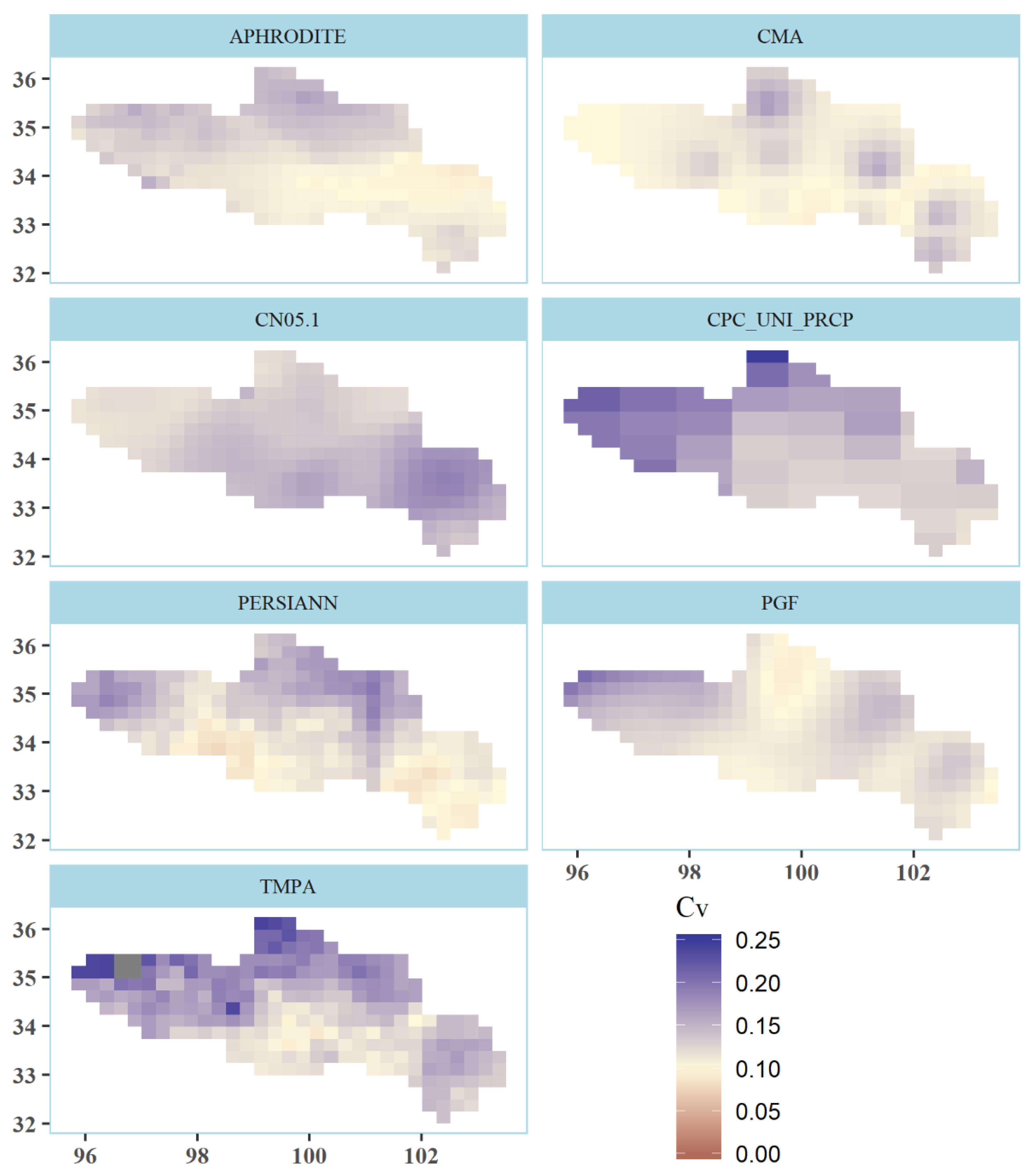
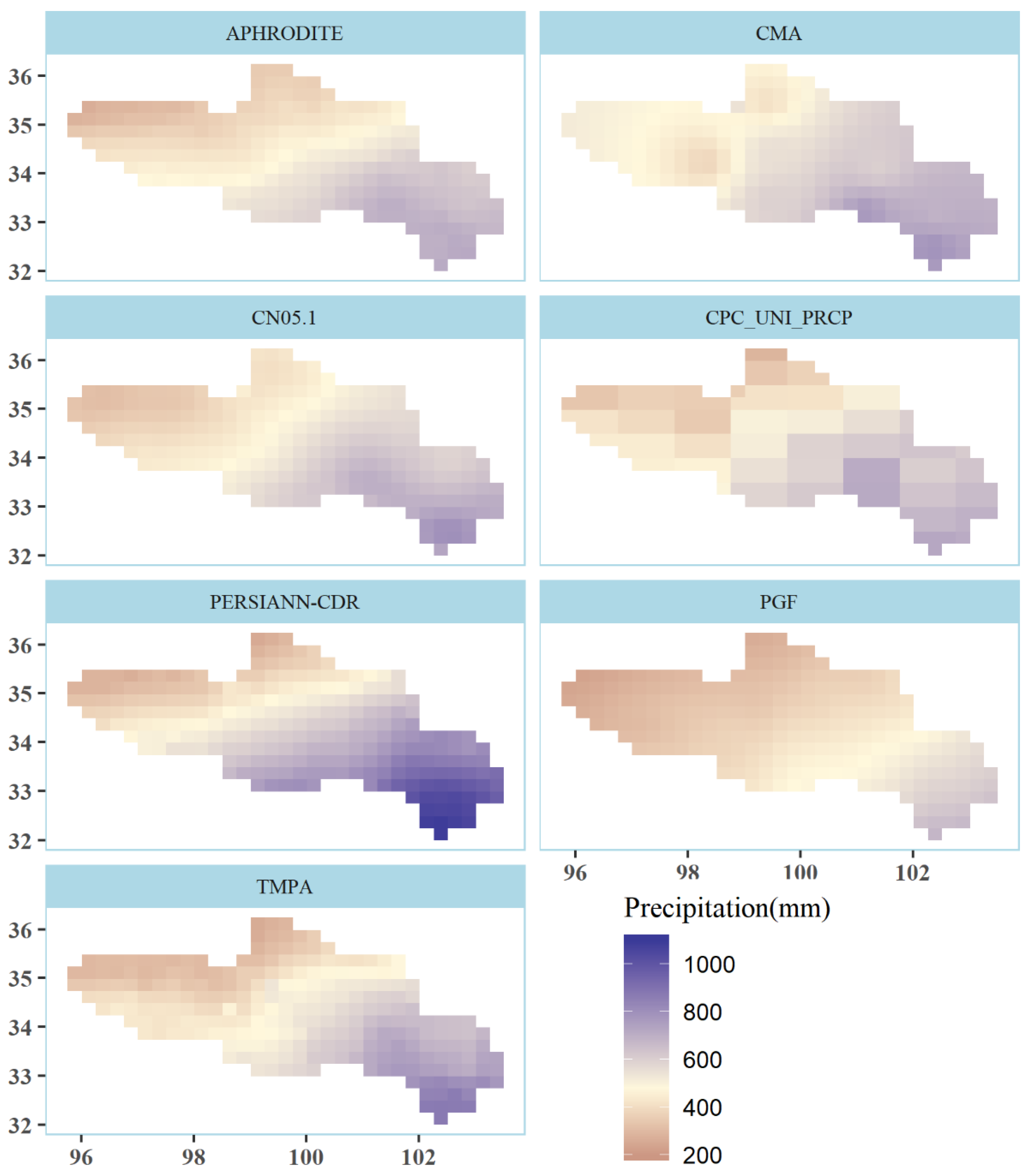
Figure 2 demonstrates the spatial pattern of the mean annual precipitation from 1998 to 2014, obtained from the CMA gauge data and 6 other estimates product over the UYRB. Furthermore, the variations coefficient (CV), which was calculated as the ratio of standard deviation and mean value of annual precipitation series at each grid over the UYRB, is depicted in Figure 3. The Cv value reflects the inter-annual fluctuations of time series and a higher value of Cv means stronger variation of series data.
Intuitively, Figure 2 shows that the precipitation patterns derived by the CMA and the 6 SDFE or RA products were visually compatible during the research period, with the precipitation intensities gradually decreasing from the eastern part of the basin to the western part, which was also similar to the published results [17,18]. Meanwhile, the amount of maximum mean annual precipitation occurred in the southeastern grid cells of the basin and the spatial variability analysis revealed that the low-altitude regions of the basin were characterized by higher spatial variability of precipitation, in comparison to the high mountainous regions (western part), partly due to the abundant moisture supply by the Indian summer monsoon from the Bay of Bengal and the orographic enhancement effect in the western part [17]. Although the SDFE or RA products represent a similar spatial trend, the PERSIANN-CDR showed a wetter pattern in the east of the watershed, with the mean annual precipitation amount over 1000 mm in some southeast grids, while PGF showed a slightly drier situation in the east part of the UYRB.
From Figure 3, which shows the spatial pattern of the variation coefficients of annual precipitation series, it could be seen that the CMA obtained the most uniform and smaller values of Cv over the whole UYRB and the higher Cv values were concentrated around the meteorological gauges (refer to Figure 1), which was mostly due to the interpolation method, and it did not take into account the orographic influence. The APHRODITE, CN05.1, and PGF showed similar spatial uniform variation pattern of Cv values to that from the CMA, using different interpolation, fusion, and correction methods, based on gauge- or observation-based datasets. Meanwhile, the satellite-derived rainfall products, like the PSERSIANN-CDR and TMPA, depict considerably finer and detailed spatial variations of the Cv values.
In addition, the CPC_UNI_PRCP represents less detailed spatial features of precipitation estimates than other products, because the CPC_UNI_PRCP estimates precipitation at a spatial resolution of 0.5 degree (seen in Figure 2 and Figure 3), instead of 0.25 degree for other SDFE or RA estimates products.

4.1.2. Precipitation at Gauge-Located Grid Cells

First, the multiple precipitation products estimates were evaluated by comparing them with the CMA gauge-based observations. Three meteorological gauges in the UYRB (black solid points with labels in Figure 1) were selected, with each located in the upper, middle, and downstream of the study area, respectively. The precipitation products estimated values at the three gauges were calculated by the average of the nearest grids. The Pearson’s correlation coefficients (r) between the daily precipitation estimates and observed values are shown in Table 5. It could be seen that the daily precipitation estimates from the APHRODITE and CN05.1 product had greater r values (most over 0.6) than other products, mainly because these two products were estimated, based on observed precipitation (the monsoon Asian and CMA gauge-based dataset, respectively) at valid stations with different interpolation methods. In addition, the CPC_UNI_PRCP and PGF had medium r values (between 0.4and 0.6), which also combined a suite of global observation-based datasets, while the PERSIANN-CDR and TMPA were satellite-based precipitation products.
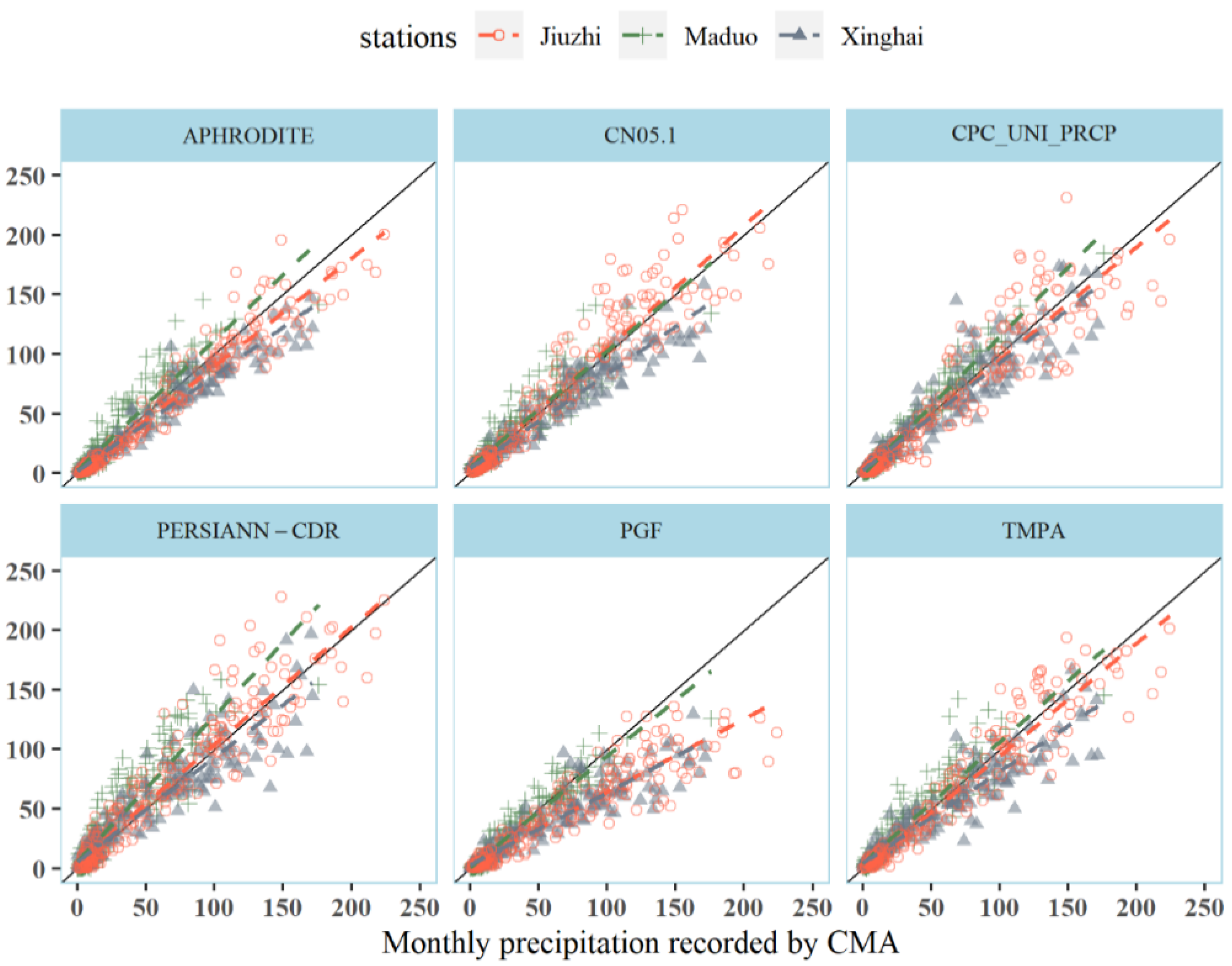
The hydrological model simulation evaluations were conducted at a monthly scale and the monthly evaluation of products estimates was conducted at the three meteorological gauges. The r, NSE0, and annual average relative error (Re) of precipitation volume are shown in Table 6. Figure 4 shows the relationship of monthly precipitation between multiple precipitation products and CMA gauge-based values. From Table 6, it could be seen that the r values were all above or close to 0.9. As for NSE0, all precipitation products showed “very good” performance (refer to Table 4 for performance rating) in monthly precipitation estimates at all three stations, with the NSE0 values over 0.75. According to Figure 4, the PGF tended to underestimate the precipitation at the Xinghai and Jiuzhi stations, with the annual relative errors being less than −10%—a “good” rating according to the Moriasi performance rating scheme.

4.1.3. Basin-Averaged Precipitation

With parsimonious hydrological models, areal average precipitation, instead of series observed at gauges, was required to drive the model. The temporal distribution and the total volume of precipitation series were also crucial components in the lumped streamflow simulation. Therefore, the areal precipitation volume was estimated in upper the four hydrometric stations, respectively, from the 7 precipitation datasets, including the gauge-based CMA and other 6 SDFE or RA products. It was unconvincing that the areal average precipitation series estimated by the CMA gauge-based dataset was much closer to the true values, especially in the gauge-sparse UYRB. Therefore, the correlation coefficient (r), instead of NSE, was selected as the performance index and calculated between the multiple precipitation products.
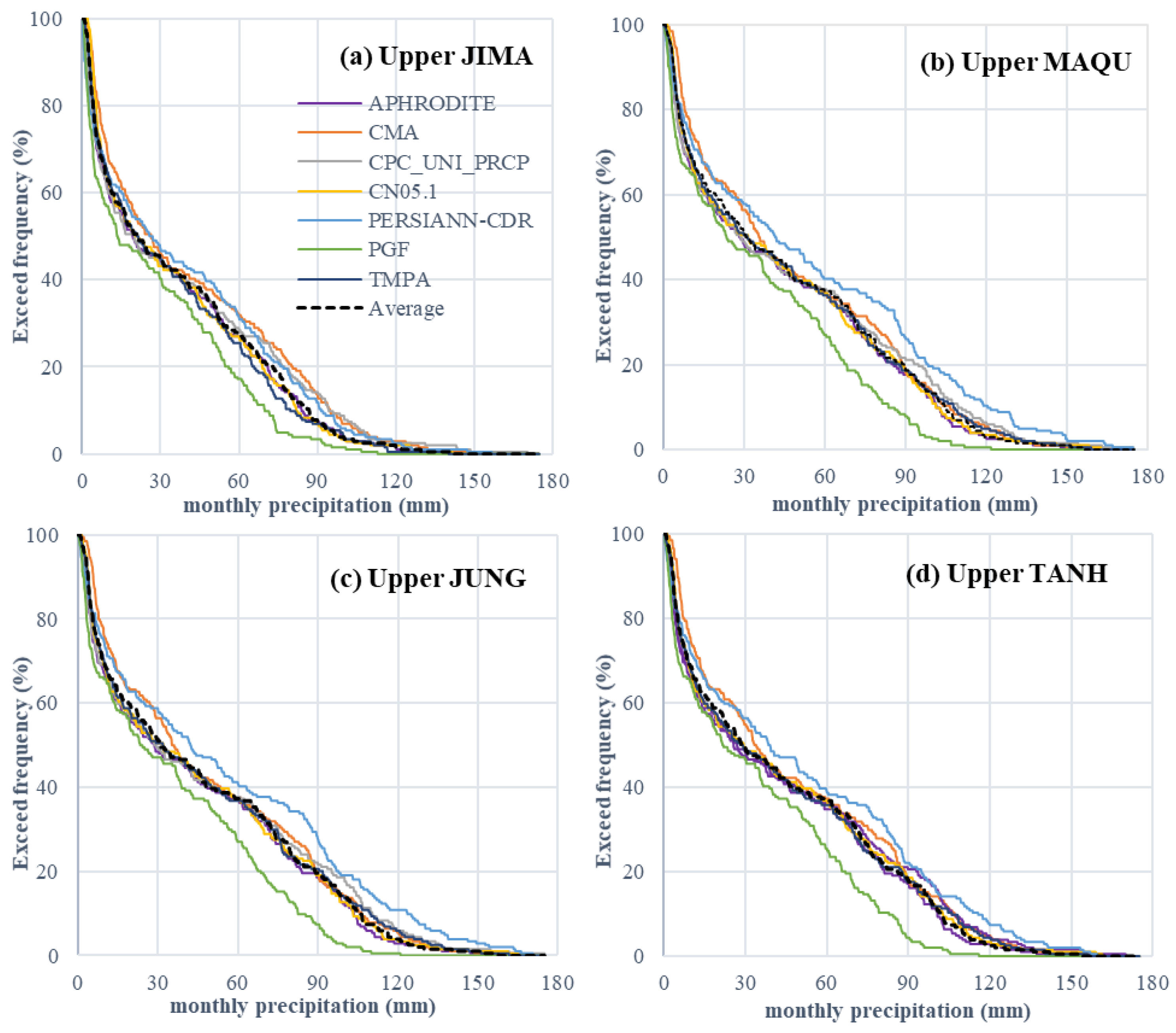
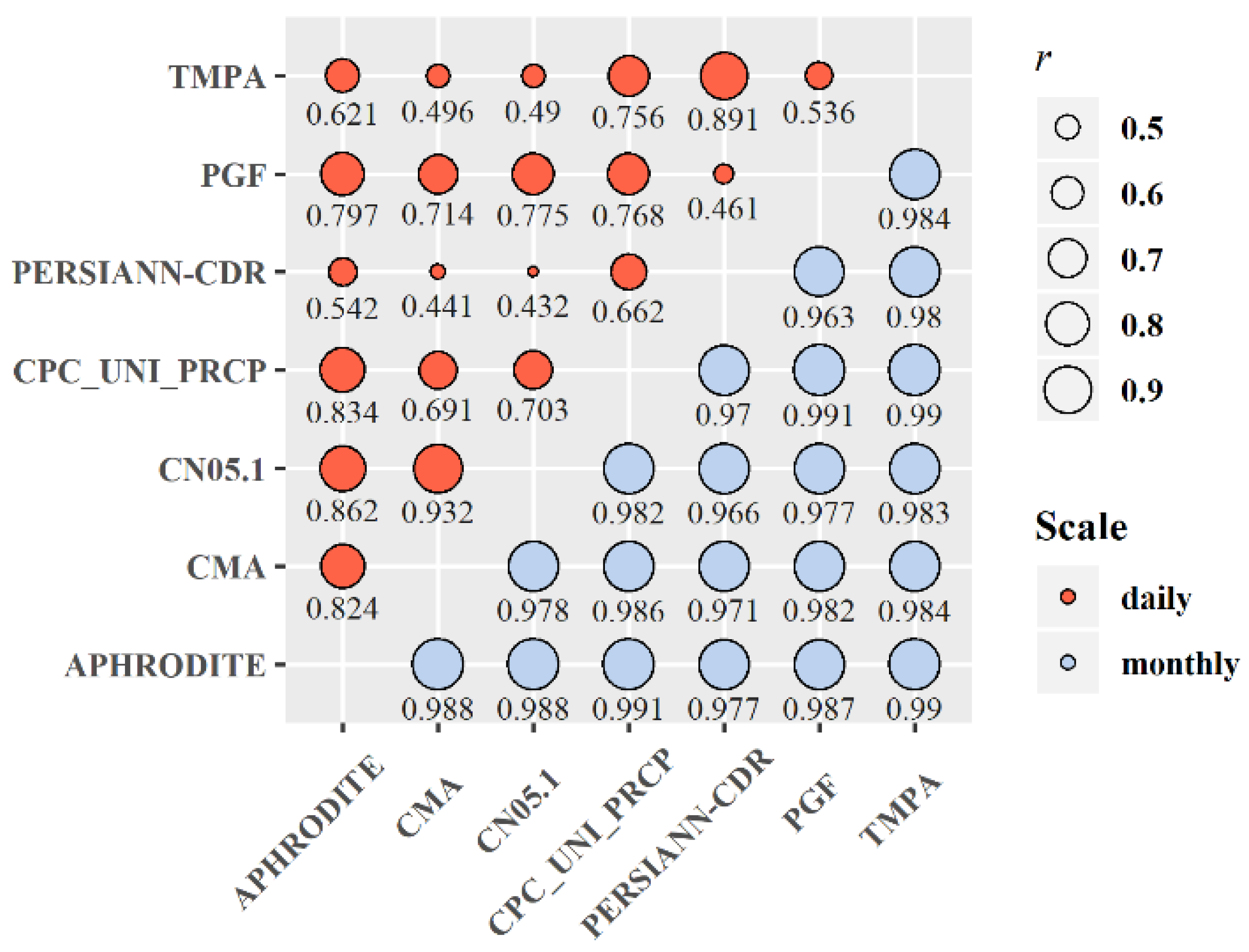
Figure 5 shows the excess frequency curves of the monthly areal average precipitation series from 7 datasets, together with the average series, where a point with the coordinates of (90, 20) meant that about 20% of the estimated monthly precipitation values were over the 90 mm. The r values of daily and monthly areal average precipitation over the whole UYRB (upper TANH station) are shown in Figure 6. Similar results were also obtained in the sub-basins, upstream of the other 3 hydrometric stations; the illustrations are omitted for brevity.
In terms of the daily precipitation estimates, the gauge-based CMA had higher r values similar to the precipitation estimates from those products corrected by or derived from daily gauge (or observation-based) datasets, such as APHRODITE, CN05.1, CPC_UNI_PRCP, and PGF, as described in Section 3.1. For the cross comparison between the monthly precipitation estimates, the r values were all above 0.9, which indicated that the overall precipitation products were consistent with each other at the monthly scale and were able to capture the seasonal distribution characteristics of precipitation in the UYRB. The excess frequency curves for the CMA, APHROFITE, CPC_UNI_PRCP, CN05.1, and TMPA were in fairly good agreement with each other and distributed near the curves for average series (black dotted lines). Additionally, the PGF dataset tended to underestimate the monthly precipitation, with the curves under the average series obviously at the lower quantile level ( 40 % ) or higher precipitation stage. The underestimation was also more noticeable for the upper MAQU, JUNG, and TANH basin, than the upper JIMA basin (source region of the UYRB, as shown in Figure 1), while the PERSIANN-CDR presents a minor overestimation of the basin-averaged precipitation.

4.2. Hydrological Evaluation of Multiple Precipitation Products

4.2.1. Monthly Streamflow Simulations

The DWBM, GR4J, RCCC-WBM, and VIC hydrological models, driven by the 7 precipitation estimates, including gauge-based CMA and other 6 SDFE or RA datasets, were used to perform streamflow simulations from 1998 to 2016, at four hydrometric stations in the UYRB. Due to the negative effects of their associated uncertainties on the hydrological modeling process, the comparative analysis was divided into two periods, which were the calibration (1998–2008) and the validation (2009–2014) periods. This was to investigate and characterize precipitation patterns and error quantification of the various precipitation estimate products over the UYRB region. Table 7 lists the mean annual runoff at 4 hydrometric stations in the UYRB, in both the calibration and validation periods. They indicate that the runoff increased a lot during the past two decades and the increase of mean annual runoff was most pronounced in the source area (JIMA station) of the UYRB, with an increment of 46.9%.
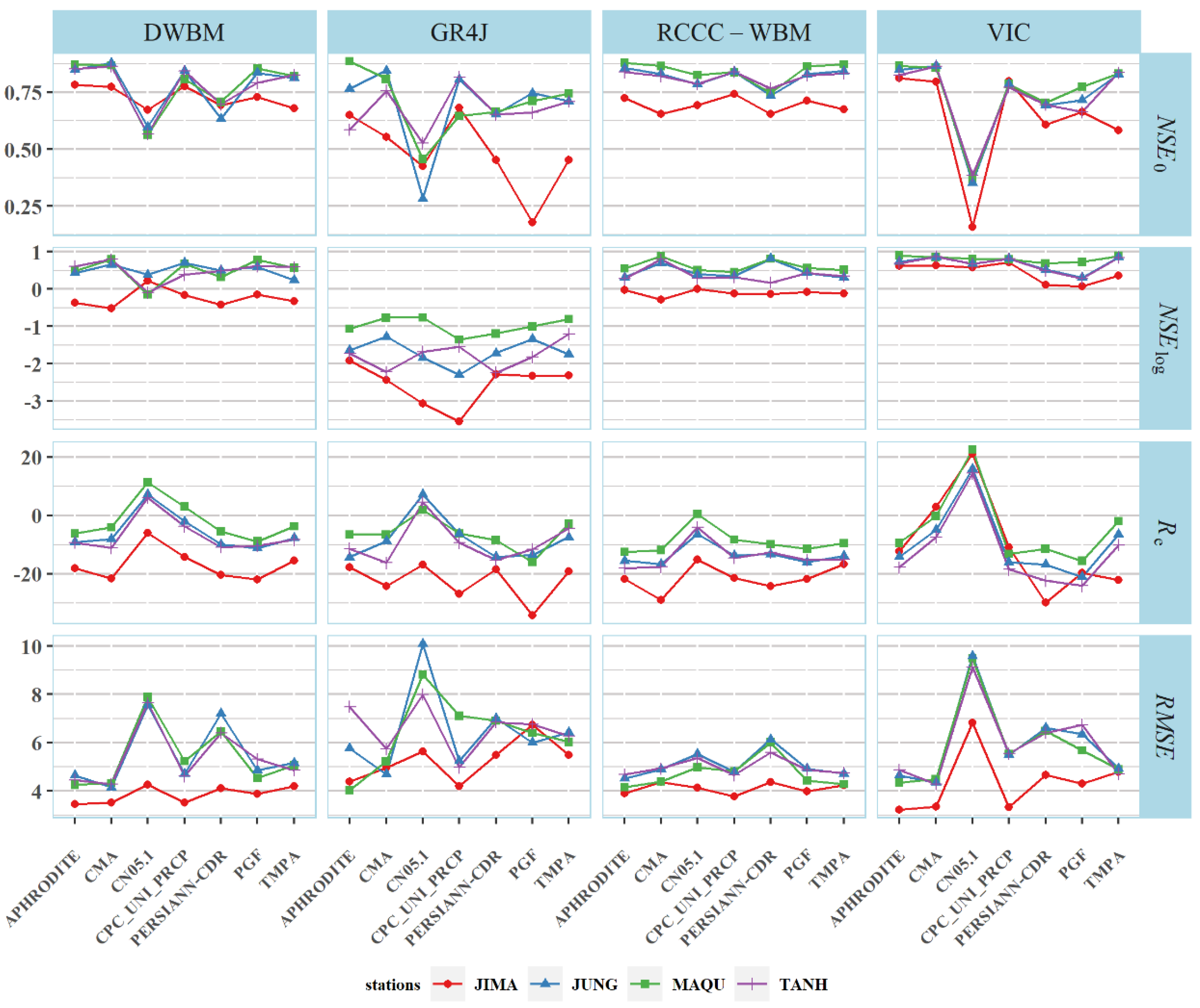
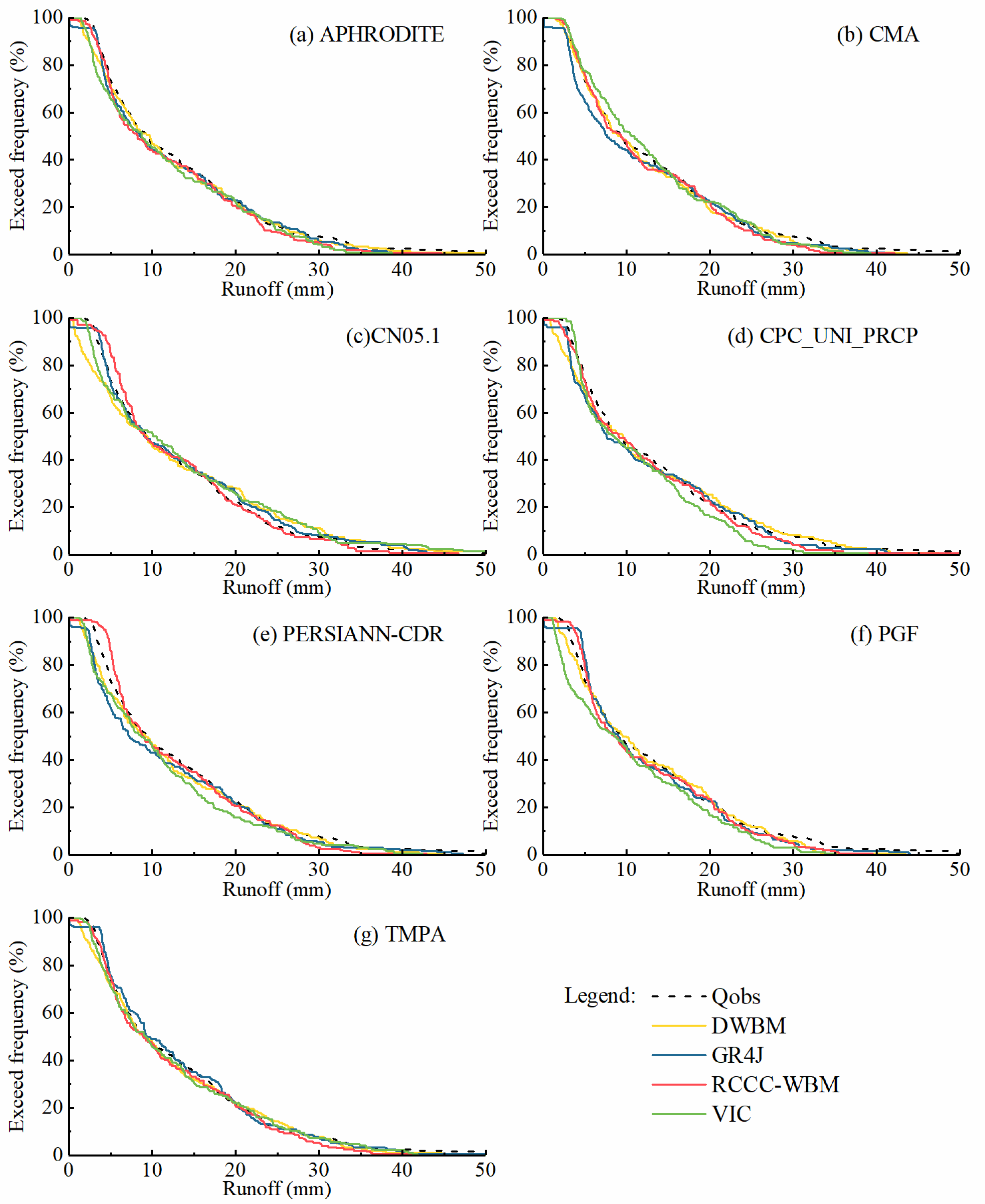
The simulated streamflow using the various precipitation inputs was compared with the observed streamflow at the monthly scale, to evaluate the hydrological utility of the satellite precipitation products, with the hydrological performance evaluation indices calculated and demonstrated in Figure 7 and Figure 8, for the calibration and validation periods, respectively. Figure 9 presents the exceed frequency curves of the simulated and observed monthly streamflow series (1998–2014), at the TANH station, as reference.
On the whole, the 7 precipitation estimates showed a great difference in monthly streamflow simulation in the UYRB, and the effects of diverse hydrological model structures in simulation performance were noticeable. In most scenarios (different precipitation products and models), the NSE0 and NSElog calculated at the validation period (2009–2014) were higher than those in the calibration period. One of the reasons might be that both rain observation gauges and satellite-based sensors had a much greater potential to capture heavy rains in the wet seasons or climate condition [16,51]. At the same time, according to previous experience, using these 4 hydrological models to simulate streamflow in humid watersheds was much better than in arid watersheds [29,32,39,52], meaning that the models might have better streamflow simulation performance in wet conditions for one watershed.
All precipitation products except the PERSIANN-CDR and CPC_UNI_PCP, showed good applicability in streamflow simulation based on the DWBM model, and obtained a “very good” rate with NSE0 over 0.75, during the calibration period. Comparing the results of simulated and observed monthly streamflow at the TANH station (Figure 9) as an illustration, the excess frequency curves for simulated streamflow, based on the 4 models driven by the APHRODITE, CMA, and TMPA precipitation estimates, were greatly consistent with that for the observed streamflow process. In this case, the relative errors in the CMA mainly occurred at the 40–80% quantile level (Figure 9b) and the CMA did not perform well at the JIMA station, mainly because there was only one rain gauge in the upper JIMA region (Figure 1), resulting in larger relative errors in basin-average precipitation estimation. The PERSIANN-CDR’s performance in streamflow simulation in the UYRB, was inferior to other precipitation products overall. The 4 hydrological models forced by the PERSIANN-CDR underestimated the streamflow at the 60–90% quantile level (low flows) and overestimated at the lower quantile level (<10%, high flows). As for the CN05.1 product, it showed good performance in the streamflow simulation in the calibration period (Figure 7), while in the validation period, the NSE0 values in the DWBM, GR4J, and VIC models dropped a lot and the Re and RMSE values increased greatly, compared to those in the calibration period (Figure 8).
From the perspective of hydrological models of different structures, the 4 selected hydrological models, used in this study on precipitation products evaluation showed great difference in reliability and stability of hydrological process simulations in the UYRB. Intuitively, the RCCC-WBM and VIC models could satisfactorily simulate the low flows in the UYRB; the NSElog values were over 0.5 at both the calibration and validation periods, and the differences in NSElog values among results from different precipitation products were small. Among the 4 hydrological models, the GR4J model showed the least stability in streamflow simulation from various precipitation estimate datasets, especially in the low-flow processes, with most NSElog values below 0 and −1, at the calibration and validation period, respectively.
The DWBM obtained a “good” performance grade in streamflow modeling, just below that of the RCCC-WBM and above that of the VIC and GR4J models. The RCCC-WBM showed the most stable and reliable streamflow simulation capacity in the UYRB, with NSE0 values between 0.7 and 0.8, NSElog over 0.5 and small Re and RMSE in both the calibration and validation periods (see Figure 7 and Figure 8). The difference and deviation between precipitation estimates from different products had little influence on the performance of the RCCC-WBM in streamflow simulation at 4 typical hydrometric stations over the UYRB. The only exception was that the results simulated by the PERSIANN-CDR precipitation estimates, based on the RCCC-WBM, were not as good as those forced by the other 6 precipitation products, mainly because of the poor performance of the PERSIANN-CDR in both the grid-based and basin-averaged precipitation estimation, as shown in Figure 4 and Figure 5. While the PGF also showed obvious errors in precipitation estimation at both gauge-located and basin-averaged scale, it obtained much better performance with higher NSE values and lower Re and RMSE than the PERSIANN-CDR in the calibration period. This might be because the PGF spatially uniformly underestimated the precipitation (Figure 4 and Figure 5) and the Cv values of annual precipitation were few and uniformly distributed (Figure 3) over the UYR. It might also be that the daily precipitation estimated by the PGF shared a better relationship (higher r values) with that obtained by the other 5 precipitation products, except the PERSIANN-CDR (Figure 6), so the RCCC-WBM had the potential to reproduce the streamflow by adjusting the model parameters to offset the negative errors in precipitation estimation by the PGF.
The streamflow process at the JIMA (the uppermost hydrometric station in the UYRB) was difficult for not only the VIC but also the other 3 conceptual hydrological models to reproduce, with lower NSE values than those at 3 other stations, in both the calibration (Figure 7) and validation (Figure 8) periods. The simulation results showed significant uncertainty at the JIMA station based on the VIC model, mainly because the VIC model was only calibrated with streamflow data observed at the TANH station, with lower NSE0 and higher Re in the period of 1998–2008, as shown in Figure 7. What was more, all 4 models showed some uncertainty and negative errors in low-flow simulation at the TANH station, namely at higher quantile levels, with excess frequency curves in Figure 9, and the phenomenon might be more noticeable at upper hydrometric stations, like the JIMA and MAQU stations. One of the reasons that the gauge-based precipitation (CMA), and SDFE or RA precipitation estimates generate smaller streamflow in the dry season or regions is the lack of a complex method or proper algorithm in the 4 models, to handle frozen soil. In dry conditions, when the amounts of precipitation and streamflow were small, the streamflow melted from frozen soil could account for a significant proportion of the total streamflow. In other words, the frozen soil melt could significantly influence the streamflow simulation results.

4.2.2. Precipitation Products Evaluation Based on Multi-Objective Optimum Fuzzy Model

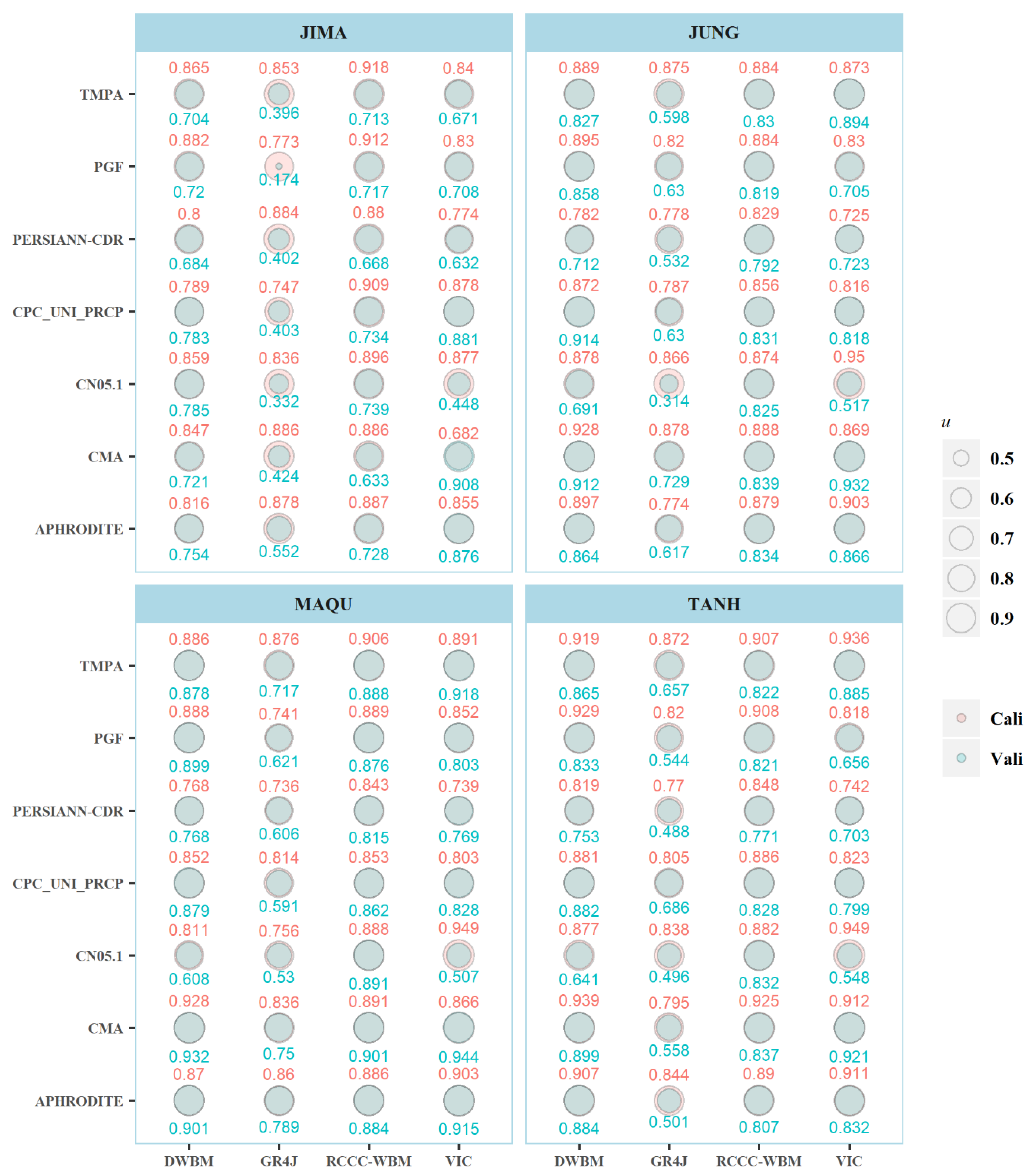
The hydrological evaluation of SDFE or RA precipitation estimates products was subject to not only the accuracy of precipitation estimates but also the structural effects of different hydrological models, as discussed in detail above. The comprehensive evaluation of precipitation products requires cross-comparison between different models. The multi-objective optimum fuzzy model was used in this research and the performance indicators are listed in Section 3.4, including two indicators reflecting the consistency and accuracy between the simulated and observed streamflow (NSE0 and NSElog), and two metrics controlling the water balance in streamflow simulation—RMSE and Re. Under the fuzzy model, the weights of the 4 metrics were assigned a vector of (0.35, 0.35, 0.15, 0.15)T ( w N S E 0 , w N S E log , w R M S E , w R e ) T , based on experts’ experience and previous studies [16]. The relative membership degree (u) of the different precipitation products at 4 hydrometric stations in both the calibration and validation periods are shown in Figure 10.
It could be seen that the two hydrological models (DWBM and RCCC-WBM), when modeling the runoff process at a monthly scale, obtained more stable and higher u values than the GR4J (daily conceptual model) and VIC models. The difference in precipitation estimates from various precipitation datasets had more influence in the GR4J and VIC models. In most scenarios, the RCCC-WBM performed best in streamflow simulation with diverse precipitation estimates sources. For the RCCC-WBM model, the u values were around 0.9 in the calibration period and 0.8 in the validation period. As for the GR4J model, the u values dropped a lot at the validation period, compared to that in the calibration period, especially at the JIMA station. Even in the calibration period, the u values obtained in the GR4J model were generally lower than those obtained by three other models, which all indicated the less suitability and high uncertainty of the GR4J model, coupled with snowmelt module in streamflow process simulation, based on the SDFE or RA precipitation datasets in the alpine UYRB. The results were similar when the hydrological processes were simulated at daily scale, with the distributed VIC model performing much better than the GR4J, with higher u values over the whole research period (1998–2014). The exception was for the CN05.1 dataset because the errors of precipitation estimates in the CN05.1 dataset after 2009 were more influential in the VIC model than the DWBM and RCCC-WBM, as shown in both Figure 8 and Figure 10.
From the perspective of precipitation products, the APHRODITE, CMA, and TMPA datasets obtained much higher scores than other datasets, with the average relative membership degree (u) values at 4 hydrometric stations from 4 hydrological models of 0.872, 0.872, and 0.887 in the calibration period and 0.787, 0.803, and 0.766 in the validation period, respectively. The precipitation estimates products (like PGF) tended to show better performance in streamflow simulation at the hydrometric stations, downstream of the UYRB (JUNG and TANH station), with an average u of 0.804 at the research period, as shown in Figure 7 and Figure 8.

4.2.3. Effect of Snowmelt Module Parameters Recalibration on Hydrological Modeling

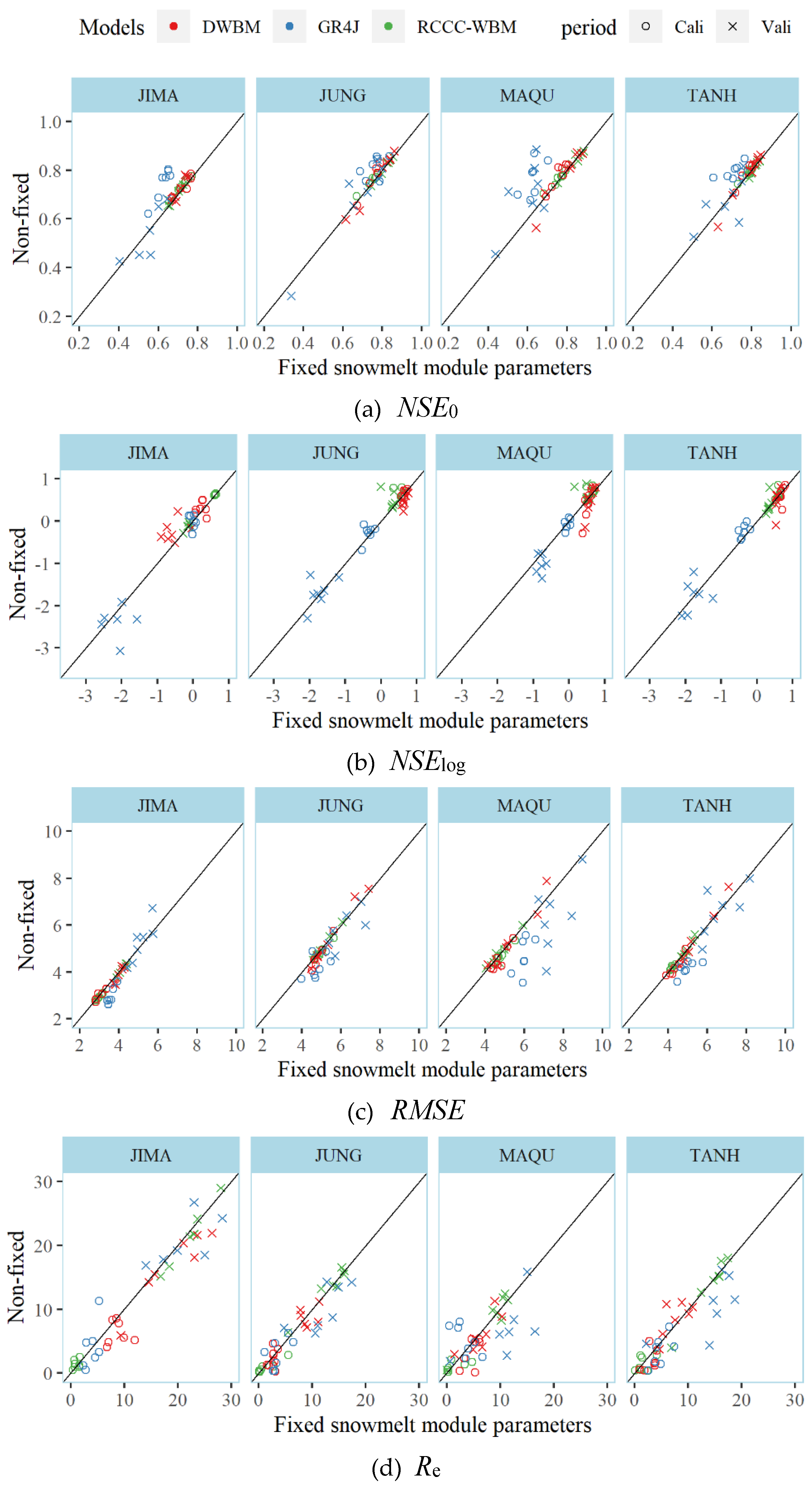
As shown above, the GR4J model showed significant uncertainty in streamflow simulation from the diverse precipitation estimates datasets. One of the reasons was that the GR4J model was forced with the daily precipitation data series, and the daily precipitation was harder to estimate accurately than monthly datasets from the SDFE or RA products. The basin-average daily precipitation data series from the 7 products showed various relationships between each other (Figure 6). On the other hand, the snowmelt modules in the DWBM and RCCC-WBM had only two parameters regulating the rainfall–snowfall partition and the two parameters were all air temperature-based, and free from the influence of watershed characteristics like the spatial pattern of snow depth. Meanwhile, the GR4J model had 4 parameters in runoff yield and routing, and incorporated the SWAT snowmelt module with 7 parameters included in model calibration, which might result in uncertainty and instability in streamflow simulation. Li et al. [39] found that little improvement was acquired when the GR4J was incorporated with the SWAT snowmelt module than the original 4 parameters GR4J model in runoff prediction in ungauged catchments. Guan, et al. [33] applied the GR4J model excluding snowmelt module in 6 typical watersheds in the Yellow River basin including the UYRB, and found that the GR4J performed well in streamflow simulation under the changing environment. Therefore, in this study, the effects of the snowmelt module were incorporated into the 3 conceptual models in hydrological evaluation of SDFE or the RA precipitation products. According to the results of the evaluation metrics as shown in Figure 7 and Figure 8, the snowmelt module parameters in the DWBM, GR4J, and RCCC-WBM models for each hydrometric station were assigned the values from the calibration results, driven by the CMA dataset and then the models’ runoff generation and routing parameters (shown in Table 3) were recalibrated with the snowmelt module parameter fixed. The evaluation metrics were calculated and compared to those (snowmelt module parameters non-fixed in model calibration) in Figure 7 and Figure 8. The comparison scatter plots are shown in Figure 11, where the shapes of the points stand for the research periods (calibration and validation) and the colors of the points distinguish the 3 hydrological models.
As shown in Figure 11, the snowmelt modules were less influential in the DWBM and RCCC-WBM models in terms of NSE0 and NSElog, with the green and red points in Figure 11a,b located in higher value ranges and near the 1:1 line (black solid line). As for the GR4J model, the blue scatter points standing for the NSE0 values in Figure 11a were mostly above the 1:1 line, meaning that the streamflow simulation capacity of the GR4J model decreased with the snowmelt module parameter fixed for each hydrometric station at the calibration period. The points below the 1:1 line mainly occurred at the validation period, which was more noticeable for NSElog in Figure 11b. In addition, the GR4J excluding the snowmelt parameter in calibration raised the RMSE metrics as some cross-shaped points were distributed above the 1:1 line. Overall, the RCCC-WBM and DWBM models, forced by monthly precipitation and potential evapotranspiration, can regulate the runoff generation amount and process, mainly based on the original model parameters. The temperature-based snowmelt modules are less influential to the simulation results. In the GR4J model, the snowmelt module (transferred from the SWAT model) played a more important role in streamflow simulation and improved the evaluation metrics in the calibration period. However, the SWAT snowmelt module also had 7 parameters, which might result in great uncertainty in model application in future runoff projection or just at the validation period.
5. Discussion

The performance of the SDFE or RA precipitation datasets in streamflow simulation was not only subjective to the precipitation estimation errors but also to the choice of different hydrological models. Normally, a certain model was employed to test and compare the applicability and precision of several precipitation products. For example, Nikolopoulos et al. [53] analyzed a number of basin scales ranging between 100 and 1200 km2, by using a distributed hydrological model, and found that the use of satellite precipitation products for flood simulation strongly depended on the catchment area and on the product resolution. Falck et al. [54] used a large-scale distributed hydrological model (MHD–INPE) to investigate the uncertainties propagation of four satellite precipitation products and error correction method in streamflow simulations. On the other hand, hydrological models are designed to deal with different hydrological and environmental issues, such as flood prediction, draught evaluation, and water resources projection [55,56], leading to great distinction in model structures, which subsequently influences the performance of SDFE or RA precipitation datasets in streamflow simulation, hence some researchers would use one certain precipitation product to study, compare, and improve the hydrological models [19,57], and also to try to extend the possible application fields of one product. For example, APHRODITE dataset was used to evaluate the improvement of the snowmelt runoff model in the Kaidu River basin in Xinjiang, China [58]. The applicability of TRMM Multi-satellite Precipitation Analysis (TMPA) 3B42V7 and the Integrated Multi-satellite Retrievals for GPM (IMERG) Final Run version 05 precipitation products was evaluated in extreme precipitation and streamflow predictions over the UYRB, by using both variable infiltration capacity model [17] and grid-based Xin’anjiang model [18].
In this study, both the performance of hydrological models and applicability of SDFE or RA precipitation datasets were evaluated and thoroughly compared over the UYRB. Two monthly hydrological models (RCCC-WBM and DWBM) that were designed to evaluate the regional water resources at the interannual and inter decadal scale, showed a better performance in water balance simulation than GR4J and VIC, which pay much more emphasis on the basic rainfall-runoff process. The large spread in model performance implies that any single model should be applied with caution, as there is a great risk of biased conclusions [19]. According to the research results and previous reports, if the application goal is streamflow reconstruction or runoff projection, based on the precipitation products in data-sparse or ungauged basins, the simple and monthly hydrological models, such as the DWBM and RCCC-WBM, are pragmatic and reliable. After all, the effective and accurate simulation of streamflow and terrestrial water resources in the UYRB, assisted by grid-based precipitation products, is the basis for developing water-management strategies at the local, regional, and national levels, which would promote both suitable industrial applications and sustainable supplies [59,60]. On the other hand, the GR4J, VIC, and other process-oriented models are highly suggested to test the accuracy, certainty, and stability of precipitation products, and the results can be used by product publishers to improve their algorithms and perform bias-correction of the SDFE or RA datasets to enhance the quality and utility.

6. Summary and Conclusions

Precipitation is one of the most important components in the hydrological cycle, and the crucial input climatic variable for regional streamflow simulation. Global satellite-based rainfall estimates (SDFE) and reanalysis precipitation (RA) products provide hydrologists with a critical precipitation data source for hydrological applications in data-sparse or ungauged basins. In this study, 6 widely used precipitation products (APHRODITE, CPC_UNI_PRCP, CN05.1, PERSIANN-CDR, PGF, and TMPA) were evaluated against gauge observations (the CMA data) and applied in streamflow simulation over the Upper Yellow River basin (UYRB), using 4 hydrological models with different structures. The main findings were as follows.
In terms of the spatial pattern of mean annual precipitation, precipitation patterns derived by the CMA and the 6 SDFE or RA products were consistent with each other. The satellite-derived rainfall products, like the PSERSIANN-CDR and TMPA, depict a considerably finer and detailed spatial heterogeneity of precipitation estimates, while the PERSIANN-CDR overestimated the mean annual precipitation in the Southeastern UYRB. The daily and monthly precipitation estimates from the products (APHRODITE, CN05.1, CPC_UNI_PRCP, and PGF) with gauge information sources combined, had higher correlation coefficients with observed precipitation series from the CMA gauges. The satellite-based products can estimate the monthly precipitation very well, at both gauge and basin-average scale.
To test the application of precipitation products in streamflow simulation at four hydrometric stations in the UYRB, the DWBM, GR4J, RCCC-WBM, and VIC were built with snow accumulation and the melting process considered in model structure. The APHRODITE and TMPA were superior to other precipitation datasets, obtaining much higher scores with the average relative membership degree (u) values at 4 hydrometric stations from 4 hydrological models of 0.872 and 0.887, at the calibration period, and 0.787 and 0.766 at the validation period, respectively. The precipitation estimates products (like PGF) tended to show better performance in streamflow simulation at the hydrometric stations, downstream of the UYRB.
In terms of performance of hydrological models, the RCCC-WBM model showed the best potential for monthly streamflow simulation, followed by the DWBM, indicating that the monthly models were more flexible than daily conceptual or distributed models in hydrological evaluation of SDFE or RA products and the difference in precipitation estimates from various precipitation datasets were more influential on the GR4J and VIC model. The GR4J model showed significant uncertainty in streamflow simulation from diverse precipitation estimate datasets. One of the reasons was that the GR4J model was forced with daily rainfall series, which were harder to estimate accurately than monthly precipitation in SDFE or RA products. In addition, the snowmelt module incorporated in the GR4J was from the SWAT model and had 7 parameters, which might also result in great uncertainty in model application.
The streamflow, recorded at hydrometric stations, was used for validating watershed hydrological models in precipitation product evaluation, as it is the integral of all hydrological processes occurring in a catchment. This work explored the ability of each precipitation dataset in simulating streamflow, based on streamflow relevant performance indicators. It would be extremely interesting to include other simulated outputs, such as soil moisture and evapotranspiration, compared against situ observations or satellite-retrieved data, to evaluate the applicability of precipitation in hydrological simulation, although the further evaluation scheme needs to be well-constructed.

Author Contributions

Conceptualization, X.G., J.Z. and G.W.; Data curation, X.T., Y.L. and Z.B.; Methodology, X.G.; Project administration, G.W.; Software, X.G. and J.J.; Supervision, G.W.; Validation, C.L. and Z.B.; Visualization, X.G.; Writing—original draft, X.G.; Writing—review & editing, Q.Y. All authors have read and agreed to the published version of the manuscript.

Funding

This study was funded by the National Key Research and Development Programs of China (Grants: 2016YFA0601501, 2017YFC0404401, 2017YFA0605002), the National Natural Science Foundation of China (Grants: 51879164,41830863, 51879162), the Second Comprehensive Scientific Investigation and Research on the Qinghai-Tibet Plateau (2019QZKK0203), and Hohai University-Basic Scientific Research Operating Expenses of Central Universities (Grants: 2013-B200203016).

Acknowledgments

We are thankful to the Chinese Meteorology Administration and Hydrology and Water Resources Survey Bureau, Qinghai Province for providing the station-based hydrometeorological data. Authors are also grateful to the three anonymous reviewers for their constructive comments and suggestions that helped improve the manuscript.

Conflicts of Interest

The authors declare no competing interests.

References

  1. Silberstein, R.P. Hydrological models are so good, do we still need data? Environ. Model. Softw. 2006, 21, 1340–1352. [Google Scholar] [CrossRef]
  2. Al-Abed, N.; Al-Sharif, M. Hydrological Modeling of Zarqa River Basin-Jordan Using the Hydrological Simulation Program-FORTRAN (HSPF) Model. Water Resour. Manag. 2008, 22, 1203–1220. [Google Scholar] [CrossRef]
  3. Machado, A.R.; Wendland, E.; Krause, P. Hydrologic Simulation for Water Balance Improvement in an Outcrop Area of the Guarani Aquifer System. Environ. Process. 2016, 3, 19–38. [Google Scholar] [CrossRef]
  4. Hu, Y.; Maskey, S.; Zhao, U.H. Streamflow trends and climate linkages in the source region of the Yellow River, China. Hydrol. Process. 2011, 25, 3399–3411. [Google Scholar] [CrossRef]
  5. Poméon, T.; Jackisch, D.; Diekkrüger, B. Evaluating the Performance of Remotely Sensed and Reanalysed Precipitation Data over West Africa using HBV light. J. Hydrol. 2017, 547, 222–235. [Google Scholar] [CrossRef]
  6. Tang, X.; Zhang, J.; Wang, G.; Yang, Q.; Yang, Y.; Guan, T.; Liu, C.; Jin, J.; Liu, Y.; Bao, Z. Evaluating Suitability of Multiple Precipitation Products for the Lancang River Basin. Chin. Geogr. Sci. 2019, 29, 37–57. [Google Scholar] [CrossRef] [Green Version]
  7. Worqlul, A.W.; Maathuis, B.; Adem, A.A.; Demissie, S.S.; Langan, S.; Steenhuis, T.S. Comparison of rainfall estimations by TRMM 3B42, MPEG and CFSR with ground-observed data for the Lake Tana basin in Ethiopia. Hydrol. Earth Syst. Sci. 2014, 18, 4871–4881. [Google Scholar] [CrossRef] [Green Version]
  8. Gebremichael, M.; Bitew, M.M.; Hirpa, F.A.; Tesfay, G.N. Accuracy of satellite rainfall estimates in the Blue Nile Basin: Lowland plain versus highland mountain. Water Resour. Res. 2015, 50, 8775–8790. [Google Scholar] [CrossRef]
  9. Thiemig, V.; Rojas, R.; Zambrano-Bigiarini, M.; De Roo, A. Hydrological evaluation of satellite-based rainfall estimates over the Volta and Baro-Akobo Basin. J. Hydrol. 2013, 499, 324–338. [Google Scholar] [CrossRef]
  10. Bitew, M.M.; Gebremichael, M. Assessment of satellite rainfall products for streamflow simulation in medium watersheds of the Ethiopian highlands. Hydrol. Earth Syst. Sci. 2011, 15, 1147–1155. [Google Scholar] [CrossRef] [Green Version]
  11. Zhu, X.; Zhang, M.; Wang, S.; Qiang, F.; Zeng, T.; Ren, Z.; Dong, L. Comparison of monthly precipitation derived from high-resolution gridded datasets in arid Xinjiang, central Asia. Quat. Int. 2015, 358, 160–170. [Google Scholar] [CrossRef]
  12. Hughes, D.A. Comparison of satellite rainfall data with observations from gauging station networks. J. Hydrol. 2006, 327, 399–410. [Google Scholar] [CrossRef]
  13. Gao, Y.; Liu, M. Evaluation of high-resolution satellite precipitation products using rain gauge observations over the Tibetan Plateau. Hydrol. Earth Syst. Sci. 2013, 17, 837–849. [Google Scholar] [CrossRef] [Green Version]
  14. Chen, M.; Xu, S.; Liu, J.; Ji, H. Temporospatial distribution of precipitation in Lhasa River basin based on TRMM data. J. China Three Gorges Univ. (Nat. Sci.) 2017, 39, 5–9. [Google Scholar]
  15. Meng, J.; Li, L.; Hao, Z.; Wang, J.; Shao, Q. Suitability of TRMM satellite rainfall in driving a distributed hydrological model in the source region of Yellow River. J. Hydrol. 2014, 509, 320–332. [Google Scholar] [CrossRef]
  16. Zhang, X.; Peng, Y.; Wang, B.; Wang, H. Suitability evaluation of precipitation data using SWAT model. Trans. Chin. Soc. Agric. Eng. 2014, 30, 88–96. [Google Scholar] [CrossRef]
  17. Su, J.; Lue, H.; Wang, J.; Sadeghi, A.M.; Zhu, Y. Evaluating the Applicability of Four Latest Satellite-Gauge Combined Precipitation Estimates for Extreme Precipitation and Streamflow Predictions over the Upper Yellow River Basins in China. Remote Sens. 2017, 9, 1176. [Google Scholar] [CrossRef] [Green Version]
  18. Yuan, F.; Wang, B.; Shi, C.; Cui, W.; Zhao, C.; Liu, Y.; Ren, L.; Zhang, L.; Zhu, Y.; Chen, T.; et al. Evaluation of hydrological utility of IMERG Final run V05 and TMPA 3B42V7 satellite precipitation products in the Yellow River source region, China. J. Hydrol. 2018, 567, 696–711. [Google Scholar] [CrossRef]
  19. Gudmundsson, L.; Tallaksen, L.M.; Stahl, K.; Clark, D.B.; Dumont, E.; Hagemann, S.; Bertrand, N.; Gerten, D.; Heinke, J.; Hanasaki, N.; et al. Comparing Large-Scale Hydrological Model Simulations to Observed Runoff Percentiles in Europe. J. Hydrometeorol. 2012, 13, 604–620. [Google Scholar] [CrossRef]
  20. Yatagai, A.; Kamiguchi, K.; Arakawa, O.; Hamada, A.; Yasutomi, N.; Kitoh, A. APHRODITE: Constructing a Long-Term Daily Gridded Precipitation Dataset for Asia Based on a Dense Network of Rain Gauges. Bull. Am. Meteorol. Soc. 2012, 93, 1401–1415. [Google Scholar] [CrossRef]
  21. Xie, P.; Yatagai, A.; Chen, M.; Hayasaka, T.; Yang, S. A Gauge-Based Analysis of Daily Precipitation over East Asia. J. Hydrometeorol. 2007, 8, 607. [Google Scholar] [CrossRef]
  22. Wu, J.; Gao, X. A gridded daily observation dataset over China region and comparison with the other datasets. Chin. J. Geophys. 2013, 56, 1102–1111. [Google Scholar]
  23. Hsu, K.; Gao, X.; Sorooshian, S.; Gupta, H.V. Precipitation Estimation from Remotely Sensed Information Using Artificial Neural Networks. J. Appl. Meteorol. 1997, 36, 1176–1190. [Google Scholar] [CrossRef]
  24. Sheffield, J.; Goteti, G.; Wood, E.F. Development of a 50-Year High-Resolution Global Dataset of Meteorological Forcings for Land Surface Modeling. J. Clim. 2006, 19, 3088–3111. [Google Scholar] [CrossRef] [Green Version]
  25. Huffman, G.J.; Bolvin, D.T.; Nelkin, E.J.; Wolff, D.B.; Adler, R.F.; Gu, G.; Hong, Y.; Bowman, K.P.; Stocker, E.F. The TRMM Multisatellite Precipitation Analysis (TMPA): Quasi-Global, Multiyear, Combined-Sensor Precipitation Estimates at Fine Scales. J. Hydrometeorol. 2007, 8, 38–55. [Google Scholar] [CrossRef]
  26. Yatagai, A.; Arakawa, O.; Kamiguchi, K.; Kawamoto, H.; Nodzu, M.; Hamada, A. A 44Year Daily Gridded Precipitation Dataset for Asia Based on a Dense Network of Rain Gauges. Sola 2009, 5, 137–140. [Google Scholar] [CrossRef] [Green Version]
  27. Xu, Y.; Gao, X.; Shen, Y.; Xu, C.; Shi, Y.; Giorgi, F. A Daily Temperature Dataset over China and Its Application in Validating a RCM Simulation. Adv. Atmos. Sci. 2009, 26, 763–772. [Google Scholar] [CrossRef]
  28. Hsu, K.-L.; Gupta, H.V.; Gao, X.; Sorooshian, S. Estimation of physical variables from multichannel remotely sensed imagery using a neural network: Application to rainfall estimation. Water Resour. Res. 1999, 35, 1605–1618. [Google Scholar] [CrossRef]
  29. Deng, C.; Liu, P.; Wang, D.; Wang, W. Temporal variation and scaling of parameters for a monthly hydrologic model. J. Hydrol. 2018, 558, 290–300. [Google Scholar] [CrossRef]
  30. Zhao, J.; Wang, D.; Yang, H.; Sivapalan, M. Unifying catchment water balance models for different time scales through the maximum entropy production principle. Water Resour. Res. 2016, 52, 7503–7512. [Google Scholar] [CrossRef]
  31. Thomas, J.R.; Harold, A. Improved Methods for National Water Assessment, Water Resources Contract: WR15249270; Harvard Water Resources Group: Cambridge, MA, USA, 1981. [Google Scholar] [CrossRef]
  32. Wang, G.Q.; Zhang, J.Y.; Jin, J.L.; Liu, Y.L.; He, R.M.; Bao, Z.X.; Liu, C.S.; Li, Y. Regional calibration of a water balance model for estimating stream flow in ungauged areas of the Yellow River Basin. Quat. Int. 2014, 336, 65–72. [Google Scholar] [CrossRef]
  33. Guan, X.; Zhang, J.; Elmahdi, A.; Li, X.; Liu, J.; Liu, Y.; Jin, J.; Liu, Y.; Bao, Z.; Liu, C. The Capacity of the Hydrological Modeling for Water Resource Assessment under the Changing Environment in Semi-Arid River Basins in China. Water 2019, 11, 1328. [Google Scholar] [CrossRef] [Green Version]
  34. Wang, G.; Zhang, J.; Yang, Q. Attribution of Runoff Change for the Xinshui River Catchment on the Loess Plateau of China in a Changing Environment. Water 2016, 8, 267–280. [Google Scholar] [CrossRef] [Green Version]
  35. Nascimento, N.D.O.; Yang, X.; Makhlouf, Z.; Michel, C. GR3J: A daily watershed model with three free parameters. Int. Assoc. Sci. Hydrol. Bull. 1999, 44, 263–277. [Google Scholar] [CrossRef]
  36. Xu, C.-Y.; Singh, V.P. A Review on Monthly Water Balance Models for Water Resources Investigations. Water Resour. Manag. 1998, 12, 20–50. [Google Scholar] [CrossRef]
  37. Perrin, C.; Michel, C.; Andréassian, V. Improvement of a parsimonious model for streamflow simulation. J. Hydrol. 2003, 279, 275–289. [Google Scholar] [CrossRef]
  38. Neitsch, S.L.; Arnold, J.G.; Kiniry, J.R.; Williams, J.R. Soil and Water Assessment Tool Theoretical Documentation Version 2009; Texas Water Resources Institute: College Station, TX, USA, 2011. [Google Scholar]
  39. Li, F.; Zhang, Y.; Xu, Z.; Liu, C.; Zhou, Y.; Liu, W. Runoff predictions in ungauged catchments in southeast Tibetan Plateau. J. Hydrol. 2014, 511, 28–38. [Google Scholar] [CrossRef]
  40. Liang, X.; Lettenmaier, D.P.; Wood, E.F.; Burges, S.J. A simple hydrologically based model of land surface water and energy fluxes for general circulation models. J. Geophys. Res. Atmos. 1994, 99, 14415–14428. [Google Scholar] [CrossRef]
  41. Lohmann, D.; Raschke, E.; Nijssen, B.; Lettenmaier, D.P. Regional scale hydrology: I. Formulation of the VIC-2L model coupled to a routing model. Hydrol. Sci. J. 1998, 43, 131–141. [Google Scholar] [CrossRef]
  42. Wi, S.; Ray, P.; Demaria, E.M.C.; Steinschneider, S.; Brown, C. A user-friendly software package for VIC hydrologic model development. Environ. Model. Softw. 2017, 98, 35–53. [Google Scholar] [CrossRef]
  43. Hansen, M.C.; Defries, R.S.; Townshend, J.R.G.; Sohlberg, R. Global land cover classification at 1 km spatial resolution using a classification tree approach. Int. J. Remote Sens. 2000, 21, 1331–1364. [Google Scholar] [CrossRef]
  44. Allen, R.D.; Pereira, L.A.S.; Raes, D.; Smith, M. Crop evapotranspiration: Guidelines for computing crop water requirements. FAO 1980, 300, D05109. [Google Scholar]
  45. Guan, X.; Zhang, J.; Yang, Q.; Wang, G. Changing characteristics and attribution analysis of potential evapotranspiration in the Huang–Huai–Hai River Basin, China. Meteorol. Atmos. Phys. 2020. [Google Scholar] [CrossRef]
  46. Nash, J.E.; Sutcliffe, J.V. River flow forecasting through conceptual models part I—A discussion of principles. J. Hydrol. 1970, 10, 282–290. [Google Scholar] [CrossRef]
  47. Moriasi, D.; Arnold, J.; Van Liew, M.; Bingner, R.; Harmel, R.D.; Veith, T. Model Evaluation Guidelines for Systematic Quantification of Accuracy in Watershed Simulations. Trans. Asabe 2007, 50. [Google Scholar] [CrossRef]
  48. Duan, Q.; Sorooshian, S.; Gupta, V.K. Effective and Efficient Gobal Optimization for Conceptual Rainfall-Runoff Models. Water Resour. Res. 1992, 28, 1015–1031. [Google Scholar] [CrossRef]
  49. Duan, Q.; Gupta, V.K.; Sorooshian, S. Shuffled complex evolution approach for effective and efficient global minimization. J. Optim. Theory Appl. 1993, 76, 501–521. [Google Scholar] [CrossRef]
  50. Duan, Q.; Sorooshian, S.; Gupta, V.K. Optimal Use of the SCE-UA Global Optimization Method for Calibrating Watershed Models. J. Hydrol. 1994, 158, 265–284. [Google Scholar] [CrossRef]
  51. Guan, X.; Jin, J.; Liu, Y.; Luo, Z.; Yang, B.; Chen, Q. Numerical weather forecast mode-based mediumterm runoff prediction of watershed. Water Resour. Hydropower Eng. 2018, 49, 46–53. [Google Scholar]
  52. Deng, P.; Wang, Y.; Hu, Q.; Liu, Y. Application of GR4J in Daily Runoff Simulation for Ganjiang River Basin. J. China Hydrol. 2014, 34, 60–65. [Google Scholar]
  53. Nikolopoulos, E.I.; Anagnostou, E.N.; Hossain, F.; Gebremichael, M.; Borga, M. Understanding the Scale Relationships of Uncertainty Propagation of Satellite Rainfall through a Distributed Hydrologic Model. J. Hydrometeorol. 2010, 11, 520–532. [Google Scholar] [CrossRef]
  54. Falck, A.S.; Maggioni, V.; Tomasella, J.; Vila, D.A.; Diniz, F.L.R. Propagation of satellite precipitation uncertainties through a distributed hydrologic model: A case study in the Tocantins-Araguaia basin in Brazil. J. Hydrol. 2015, 527, 943–957. [Google Scholar] [CrossRef]
  55. Mohammad, A.H.; Jung, H.C.; Odeh, T.; Bhuiyan, C.; Hussein, H. Understanding the impact of droughts in the Yarmouk Basin, Jordan: Monitoring droughts through meteorological and hydrological drought indices. Arab. J. Geosci. 2018, 11, 103. [Google Scholar] [CrossRef] [Green Version]
  56. Givati, A.; Thirel, G.; Rosenfeld, D.; Paz, D. Climate change impacts on streamflow at the upper Jordan River based on an ensemble of regional climate models. J. Hydrol. Reg. Stud. 2019, 21, 92–109. [Google Scholar] [CrossRef]
  57. Beck, H.E.; van Dijk, A.I.J.M.; de Roo, A.; Dutra, E.; Fink, G.; Orth, R.; Schellekens, J. Global evaluation of runoff from 10 state-of-the-art hydrological models. Hydrol. Earth Syst. Sci. 2017, 21, 2881–2903. [Google Scholar] [CrossRef] [Green Version]
  58. Li, L.; Shang, M.; Zhang, M.; Ahmad, S.; Huang, Y. Snowmelt runoff simulation driven by APHRODITE precipitation dataset. Adv. Water Sci. 2014, 25, 53–59. [Google Scholar]
  59. Hussein, H.; Menga, F.; Greco, F. Monitoring Transboundary Water Cooperation in SDG 6.5.2: How a Critical Hydropolitics Approach Can Spot Inequitable Outcomes. Sustainability 2018, 10, 3640. [Google Scholar] [CrossRef] [Green Version]
  60. da Silva, L.P.B.; Hussein, H. Production of scale in regional hydropolitics: An analysis of La Plata River Basin and the Guarani Aquifer System in South America. Geoforum 2019, 99, 42–53. [Google Scholar] [CrossRef]
Figure 1. Topographical features, river networks, and hydrometeorological gauges in the Upper Yellow River Basin (UYRB).
Remotesensing 12 04023 g001
Figure 2. Spatial distribution of mean annual precipitation estimates (unit: mm) in the period 1998–2014 from the CMA gauge-based precipitation and 6 other SDFE or RA precipitation products.
Remotesensing 12 04023 g002
Figure 3. Spatial distribution of variation coefficients (CV) of annual precipitation estimates in the period 1998–2014 from CMA gauge-based estimates and 6 other SDFE or RA precipitation estimate products, where Cv is the ratio between standard deviation and mean value.
Remotesensing 12 04023 g003
Figure 4. Scatter plot of monthly precipitation (1998–2014) between multiple precipitation products and CMA gauge-based values at three typical gauges in the UYRB.
Remotesensing 12 04023 g004
Figure 5. Exceed frequency curves of monthly basin-averaged precipitation upper (a) JIMA, (b) MAQU, (c) JUNG, and (d) TANH hydrometric station, where the average series are calculated based on CMA and other 6 precipitation products.
Remotesensing 12 04023 g005
Figure 6. Correlation coefficients (r) between the areal average precipitation over the whole UYRB calculated by the 8 precipitation products at a daily and monthly scale.
Remotesensing 12 04023 g006
Figure 7. Results of hydrological modeling performance evaluation indices (NSE0, NSElog, Re, and RMSE) in the calibration period (1998–2008) at 4 hydrometric stations (JIMA, MAQU, JUNG, and TANH), using 4 hydrological models (DWBM, GR4J, RCCC-WBM, and VIC).
Remotesensing 12 04023 g007
Figure 8. Results of hydrological modeling performance evaluation indices (NSE0, NSElog, Re, and RMSE) in the validation period (2009–2014) at 4 hydrometric stations (JIMA, MAQU, JUNG, and TANH), using 4 hydrologic models (DWBM, GR4J, RCCC-WBM, and VIC).
Remotesensing 12 04023 g008
Figure 9. Comparison of simulated and observed monthly runoff at TANH during 1998–2014 based on the precipitation estimates from (a) APHRODITE, (b) CMA, (c) CN05.1, (d) CPC_UNI_PRCP, (e) PERSIANN-CDR, (f) PGF, and (g) TMPA, respectively.
Remotesensing 12 04023 g009
Figure 10. Relative membership degree (u) of different precipitation products at 4 stations by 4 hydrological models, where the red and cyan numbers above and below the bubble points indicate the u values at the calibration (Cali, 1998–2008) and validation (Vali, 2009–2014) period, respectively.
Remotesensing 12 04023 g010
Figure 11. Comparison of performance indices (a) NSE0, (b) NSElog, (c) RMSE, and (d) Re between the simulated and observed monthly streamflow from the simulation results, using the DWBM, RCCC-WBM, and the GR4J model with fixed and non-fixed snowmelt module parameters in model calibration, based on the SCE-UA algorithm (the black line is the 1:1 reference curve).
Remotesensing 12 04023 g011
Table 1. Hydrometric gauges in the UYRB.
Hydrometric GaugesAbbreviationElevation (m)Upper Area (km2)Annual Average Discharge (m3/s)
JimaiJIMA397045,019123.4
MaquMAQU347086,048413.4
JungongJUNG338098,414493.3
TangnaihaiTANH2760121,972580.3
Table 2. The selected satellite-based or reanalysis precipitation products.
Precipitation ProductTemporal CoverageSpatial CoverageSpatial ResolutionReferenceSources
APHRODITE1951–2015Monsoon Asian0.25°Yatagai, et al. [20]JAXA
CPC_UNI_PRCP1979–2016Global0.5°Xie, et al. [21]NOAA
CN05.11961–2015China0.25°Wu and Gao [22]National Climate Center of China
PERSIANN-CDR1983-present60°S-60°N0.25°Hsu, et al. [23]University of California, Irvine
PGF1948–2016Global0.25°Sheffield, et al. [24]Princeton University
TMPA1998-present50°S–50°N0.25°Huffman, et al. [25]NASA
Table 3. The four hydrological models and their parameters.
ModelsTemporal ScaleStructureNo.ParametersDescriptionUnitPrior Range
DWBMMonthlyLumped3kInitial evaporation ratio-(0, 1)
mInitial evapotranspiration opportunity ratio-(0, 1)
SbCatchment storage capacitymm[40, 400]
RCCC-WBMMonthlyLumped4KsSurface flow coefficient-[0.1, 0.6]
KgGroundwater flow lag coefficient-[0.01, 0.2]
KsnSnowmelt driven runoff coefficient-[0.001, 0.1]
SmaxMaximum soil moisture storemm[40, 400]
GR4JDailyLumped4x1Maximum capacity of the production storemm[100, 1200]
x2Groundwater recharge coefficient-[−5, 3]
x3One day ahead maximum capacity of the routing storemm[20, 300]
x4Time base of unit hydrographdays[1.1, 2.9]
VICDailyDistributed6bVariable infiltration curve parameter-[0.00001, 0.9]
DsFraction of Dsmax where non-linear baseflow begins-(0, 0.9]
DsmaxMaximum velocity of baseflowmm/d(0, 30]
WsFraction of maximum soil moisture where non-linear baseflow begins-[0.1, 0.99]
d2Thickness of middle soil moisture layerm[0.3, 1.5]
d3Thickness of bottom soil moisture layerm[0.5, 2]
No. indicates the number of parameters (excluding the snowmelt module).
Table 4. The Moriasi performance rating scheme in watershed streamflow simulation.
Performance RatingNSERe(%)
Very good(0.75, 1.00]<±10
Good(0.65, 0.75][±10, ±15]
Satisfactory(0.50, 0.65][±15, ±25]
Unsatisfactory<0.5≥±25
Table 5. Correlation coefficients (r) between precipitation products and gauged-based observations at 3 meteorological station at daily scale.
StationAPHRODITECN05.1CPC_UNI_PRCPPERSIANN-CDRPGFTMPA
Maduo0.5760.6320.5640.3090.4590.261
Xinghai0.6890.7920.4180.2900.5080.216
Jiuzhi0.7520.7810.5200.3000.4720.307
Table 6. Correlation coefficients (r), NSE0, and relative errors (Re, unit: %) between precipitation products and gauged-based observations at 3 meteorological stations at a monthly scale.
IndicesStationAPHRODITECN05.1CPC_UNI_PRCPPERSIANN-CDRPGFTMPA
NSE0Maduo0.8090.8170.9140.8470.9130.801
Xinghai0.9020.8970.8850.8650.6840.857
Jiuzhi0.9240.8510.8540.8580.6350.907
rMaduo0.9420.9230.9840.9120.9570.925
Xinghai0.9730.9650.9420.9300.9330.944
Jiuzhi0.9690.9420.9300.9370.9220.955
ReMaduo5.914.364.2614.1−1.455.04
Xinghai−5.32−4.15−1.59−0.04−11.5−4.68
Jiuzhi−3.672.44−1.552.39−11.7−2.01
Table 7. Mean annual runoff (mm) at 4 hydrometric stations in two periods.
Station1998–20082009–2014Increment (%)
JIMA80.29117.9446.9
MAQU143.97179.6924.8
JUNG146.94192.0130.7
TANH141.35183.0929.5
Publisher’s Note: MDPI stays neutral with regard to jurisdictional claims in published maps and institutional affiliations.