Evapotranspiration Partitioning at Field Scales Using TSEB and Multi-Satellite Data Fusion in The Middle Reaches of Heihe River Basin, Northwest China

Abstract

Daily evapotranspiration (ET) and its components of evaporation (E) and transpiration (T) at field scale are often required for improving agricultural water management and maintaining ecosystem health, especially in semiarid and arid regions. In this study, multi-year daily ET, E, and T at a spatial resolution of 100 m in the middle reaches of Heihe River Basin were computed based on an ET partitioning method developed by combing remote sensing-based ET model and multi-satellite data fusion methodology. Evaluations using flux tower measurements over irrigated cropland and natural desert sites indicate that this method can provide reliable estimates of surface flux partitioning and daily ET. Modeled daily ET yielded root mean square error (RMSE) values of 0.85 mm for cropland site and 0.84 mm for desert site, respectively. The E and T partitioning capabilities of this proposed method was further assessed by using ratios E/ET and T/ET derived from isotopic technology at the irrigated cropland site. Results show that apart from early in the growing season when the actual E was reduced by plastic film mulching, the modeled E/ET and T/ET agree well with observations in terms of both magnitude and temporal dynamics. The multi-year seasonal patterns of modeled ET, E, and T at field scale from this ET partitioning method shows reasonable seasonal variation and spatial variability, which can be used for monitoring plant water consumption in both agricultural and natural ecosystems.

1. Introduction

Approximately one-third of Earth’s land surface is occupied by semiarid and arid regions, where limited water resources makes it very challenging to provide industrial, agricultural, and ecological water use requirements. In many of these regions, most of the pressures on water resources is driven by evapotranspiration (ET) or water use by irrigated agriculture, which consumes nearly 80% of water resources from open water bodies and aquifers [1,2]. Increasing water consumption from agricultural irrigation results in serious degradation of natural vegetation in many of inland river basins in regions of water scarcity [3]. There is a pressing need to improve agricultural irrigation management to enhance water use efficiency in semiarid and arid regions.

For ET partitioning, transpiration (T) from crops is beneficial water use associated with crop production while evaporation (E) from bare soil is regarded as wasted water from an agronomic point of view [4,5]. Thus, the water efficient agricultural irrigation management strategy is to maximize T and minimize E. To utilize and manage water resources rationally and maintain ecosystem health in semiarid and arid regions, accurate spatiotemporal patterns of ET and its partitioning between E and T at field scale are required to assess and monitor the spatial and temporal distribution of regional water use and stress [6,7].

Over the last few decades, much research has been undertaken to quantify regional ET using remote sensing data over a wide range of temporal and spatial scales and climate conditions [8,9,10]. However, partitioning ET to E and T has mainly been achieved by measurement methods, such as micro-lysimeter, sap-flow, and isotropic analyzer [4,11,12]. Micrometeorological methods using eddy covariance measurements of water vapor and CO₂, however, have also emerged (e.g., Scanlon and Kustas, [13]) and continue to be refined and improved [14]. Nonetheless, these measurement methods not only require complex instrumentation and data processing, they are also difficult to extrapolate from local patch scale to larger spatial scales [5,15].

A limited number of remote sensing-based models have been developed to estimate ET and its components E and T at large spatial scales by using land surface parameters (e.g., land surface temperature (LST), leaf area index (LAI), and fractional vegetation cover ($f_c$)) derived from satellite observations. Such remote sensing-based models include the two source energy balance (TSEB) model [16,17], the Priestley–Taylor Jet Propulsion Lab (PT-JPL) model [18], the Global Land Evaporation Amsterdam (GLEAM) model [19], and the Penman–Monteith moderate resolution imaging spectroradiometer (PM-MODIS) [20]. Most of these models have been applied to accurately estimate ET at regional and global scales, but E and T partitioning capabilities of these models are rarely evaluated [15]. The TSEB model originally proposed by Norman et al. [16] and subsequent versions have been applied widely to partitioning ET to E and T under wide range of spatial scales and environmental conditions [5,17,21,22,23,24].

For agricultural water management and ecosystem health assessment, time-continuous ET and components E and T at field or finer scales (≤ 100 m) are required to provide detailed information about water use [22,25]. Unfortunately, time-continuous values at field scale cannot be directly computed using a single satellite system, because no single satellite system is capable of providing optical and thermal-infrared observations at both high spatial and high temporal resolutions.

Recently, efforts have been made to estimate time-continuous daily ET at field scales based on multi-satellite data fusion combined with remote sensing-based ET models [26,27]. The existing studies for estimating time-continuous daily ET at field scales can be divided into two main categories: (1) ET fusion scheme and (2) input parameter fusion scheme. The first scheme achieves daily ET at field scales via fusing modeled multi-scale ET products using remote sensing data from satellites with high spatial resolution (e.g., Landsat) and satellites with high temporal resolution (e.g., MODIS) [7,22,25,26,28,29,30,31,32,33]. In the second scheme, daily field-scale ET is directly estimated based on remote sensing-based ET models (e.g., TSEB and surface energy balance system (SEBS)) using input parameters with high spatiotemporal resolution, which is fused from multiple satellite sensors [27,34,35,36]. Both schemes have been successfully used to estimate daily field-scale ET over rainfed and irrigated agricultural areas [22,25,28,29,33,35,36], forested landscapes [31,32,35,36], and vineyards [7,30]. Ma et al. [36] reported that both schemes perform similarly for homogeneous surfaces while the input parameter fusion scheme may have slightly better performance for heterogeneous surfaces. In these previous studies, the spatial and temporal adaptive reflectance fusion model (STARFM) [37] has been widely applied for producing ET and input parameters of ET models with high spatiotemporal resolution [7,22,25,26,29,30,31,32,33,35].

Although daily field-scale ET has been achieved over different landscapes and environmental conditions in these previous studies, there are only a few studies estimating daily field-scale E and T based on multi-satellite data fusion. Following the basic scheme of estimates of daily field-scale ET, an ET partitioning method based on TSEB and STARFM is proposed for estimating daily field-scale E and T in this study. The ET partitioning method is applied to estimate daily field-scale ET, E, and T using MODIS and Landsat data collected over an arid region in China, which is mainly covered by irrigated cropland and sparsely vegetated desert. Moreover, the performance of this method is assessed by comparing modeled and measured instantaneous turbulence fluxes and daily ET for irrigated cropland and desert steppe, and by comparing modeled and measured ratio of E and T to ET over irrigated cropland. Furthermore, spatiotemporal water consumption of study area is analyzed using ET, E, and T maps at field scale produced using this ET partitioning method.

2. Materials and Methods

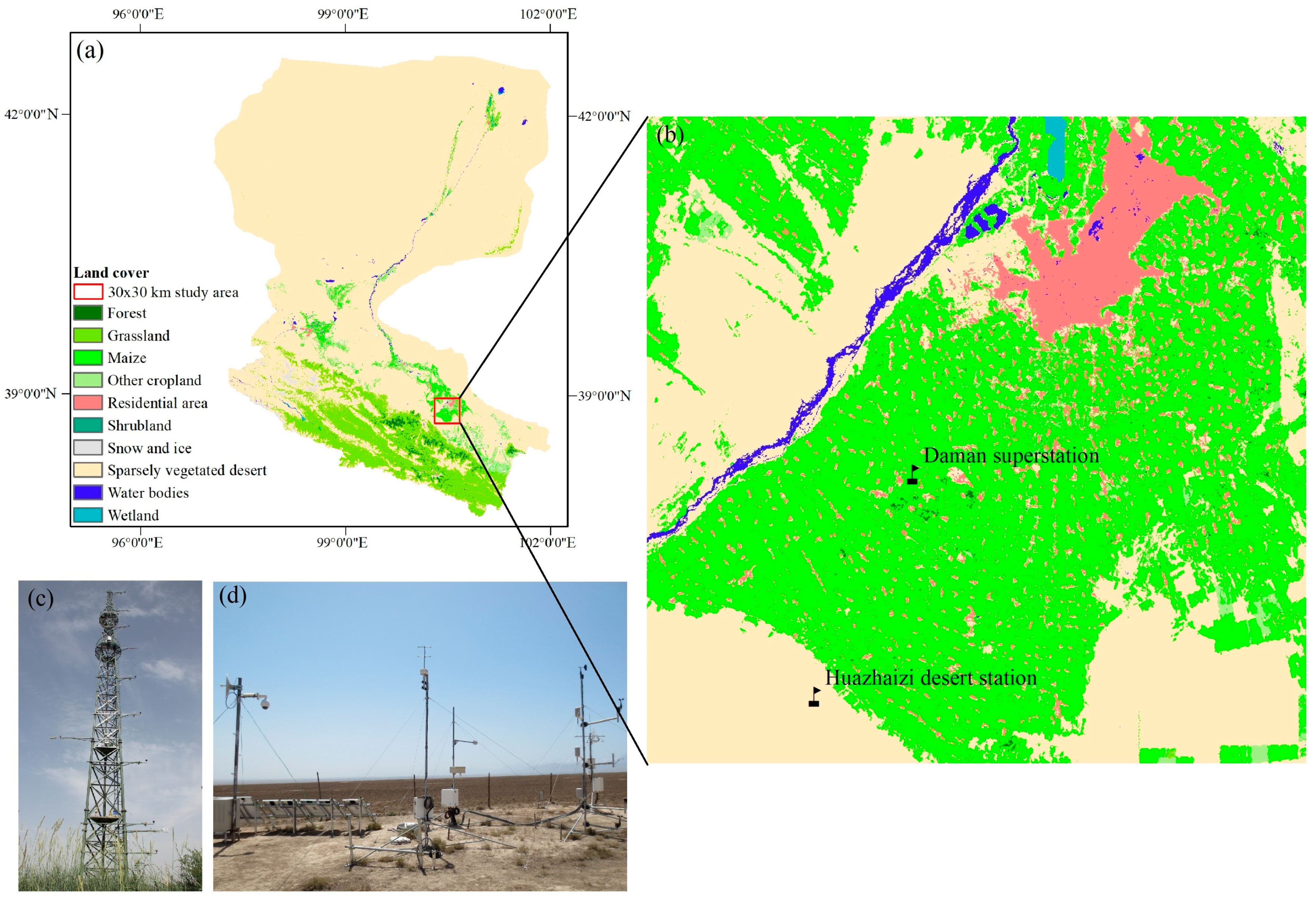
2.1. Study Area

The evapotranspiration partitioning method was applied in a desert–oasis zone, which is located in the middle reaches of Heihe River Basin in northwest China, as shown in Figure 1. This study area is 30 km × 30 km characterized by sparsely vegetated desert (36%), and an artificial oasis (>60%) dominated by irrigated maize, vegetables, residential areas, orchards, and poplar shelterbelts. This study area has an arid continental monsoon climate characterized by rainy summers and dry winters with over 60% of precipitation occurring in the summer [38]. The annual mean air temperature is approximately 6–8 °C [39] and the annual precipitation is about 100–250 mm, while the annual potential evaporation ranges from 1200 mm to 1800 mm [40]. The water resources for this area are the Heihe River and groundwater [39]. There is considerable amount of water consumed by irrigated cropland surrounded by desert creating an oasis type setting. Given that a fraction of the irrigated water is lost via soil evaporation and therefore not used in crop biomass accumulation, accurately partitioning of evapotranspiration into evaporation and transpiration is crucial to evaluate strategies for reducing E that will lead to water conservation.

In 2012, the Heihe Watershed Allied Telemetry Experimental Research–Multi-Scale Observation Experiment on Evapotranspiration (HiWATER-MUSOEXE) was launched for studying the spatial-temporal variations as well as the impact factors of ET within this desert–oasis ecosystem [41,42,43,44]. In HiWATER-MUSOEXE experiment, the intensive observations of ET and atmospheric and biophysical data were collected over this study area between 3 May and 21 September in 2012 [42], while long term observations of ET in cropland and desert steppe have continued since 2012 [41].

2.2. Field Measurements

Two study sites, Daman superstation (DM) and Huazhaizi desert station (HZZ), for obtaining long-term observations in HiWATER-MUSOEXE were selected for applying and evaluating estimates of ET and ET partitioning in this study, as shown in Figure 1.

The Daman superstation (Figure 1c) is located in cropland covered by seeded maize, which is usually planted in late April and harvested in late September. In the early stage of growth, the maize grows quickly and reaches its maximum canopy height (~2 m) and LAI (~4.5) at the end of June [23]. The soil moisture in this cropland is relatively high (ranges from 0.2 to 0.5 m³/m³) due to flood irrigation and precipitation during the whole growing season [23]. To reduce the loss of evaporated water from the soil surface for improving water use efficiency, plastic films are used in this cropping system. The plastic films cover approximately 60% of the soil surface. The Huazhaizi desert site (Figure 1d) is located in a natural desert steppe dominated by perennial short shrub-Reaumuria soongaria with constant canopy height of 0.3 m, maximum LAI of ~0.7, and soil moisture ranging between 0.07 and 0.2 m³/m³ [45].

At each site, a tower-based observation system is installed and is still in operation, which includes a four-component radiometer, automated weather stations (AWSs), eddy covariance (EC) systems, and soil heat flux plates, and soil moisture and temperature measurement systems (SMTMS) buried around the EC tower. The meteorological observations for model input and surface fluxes for model evaluation span from 1 May to 31 October for the years 2012–2016 were extracted from the HiWATER-MUSOEXE data archive at the Cold and Arid Regions Science Data Center at Lanzhou (http://card.westgis.ac.cn/).

A detailed description of all weather and surface energy balance measurements is provided in Xu et al. [44] and Liu et al. [41]. A brief description of the measurements used in this study is provided here. Meteorological data including air temperature, air pressure, wind speed and direction, and humidity at height of 5 m above ground level (agl) for DM and 3 m agl for HZZ were obtained from AWSs at 10 min averaging intervals. The four components of radiation (incoming and outgoing shortwave and longwave radiation) at height of 12 m agl for DM and 2.65 m agl for HZZ were measured by a 4-way radiometer at 10 min averaging intervals. The surface soil heat flux was calculated using heat flux plate measurements at a depth of 0.06 m combined with soil moisture and temperature at a depth of 0.02 m and 0.04 m measured by SMTMS at 10 min averaging intervals based on the one-dimensional equation of soil thermal diffusion [46]. The surface soil heat flux, radiation observations, and meteorological data were processed to 30 min averages.

The sensible ($H$) and latent ($LE$) heat fluxes used to evaluate the accuracy of modeled turbulent fluxes and daily ET were measured from EC systems installed at 4.5 m agl for DM and 2.85 m agl for HZZ. The EC system consists of an open-path infrared gas analyzer and a 3-D sonic anemometer with a sampling frequency of 10 Hz. The high frequency data collected from EC system were processed to produce 30 min average turbulent fluxes of sensible and latent heat and net carbon flux exchange using Edire software (http://www.geos.ed.ac.uk/abs/-research/micromet/EdiRE/). For more details of the EC instrumentation and processing of the 10 Hz data, please refer to Liu et al. [43] and Xu et al. [44].

Generally, the sum of $H$ and $LE$ from EC system is less than the difference between net radiation ($R_n$) measured from radiometer and the ground soil heat flux ($G$) calculated from soil heat plates, as known as surface energy imbalance or lack of energy balance closure. The average closure ratios (i.e., $\left(H+LE\right)/\left(R_n-G\right)$) during study periods for DM and HZZ were 0.80 and 0.79, respectively. To compare with the modeled fluxes, which requires energy conservation, energy balance closure was imposed on the observed fluxes. Given that the surface energy imbalance is mainly associated with underestimation of $LE$ from EC systems [47], the forced closure fluxes were achieved by using the residual-LE closure method (assigning the residual ($R_n-G-H-LE$) to observed $LE$) [48].

Measurements of ${\delta }^{18}O$ of ecosystem water pools and their flux ratios from an isotropic analyzer were obtained to evaluate the accuracy of partitioned $E$ and $T$ at Daman superstation from 27 May to 21 September in 2012 during HiWATER-MUSOEXE experiment [12]. In this study, the ratio of $E$ from soil and $T$ from maize canopy to the total ET from cropland ($E/ET$ and $T/ET$) were directly computed by Wen et al. [12] using the isotope method, which is based on the isotopic compositions of water fluxes from soil, foliage, and composite land surface. According to Wen et al. [12], the isotopic compositions of ET (${\delta }_{ET}$) was determined by flux-gradient technique, the isotopic composition of $E$ (${\delta }_E$) was calculated using Craig–Gordon model, and the composition of $T$ (${\delta }_T$) was estimated based on xylem water under isotopic steady state assumption. Finally, $E/ET$ and $T/ET$ were estimated by conservation principles based on ${\delta }_{ET}$, ${\delta }_E$, and ${\delta }_T$.

2.3. Model Inputs

The ET partitioning method based on TSEB and data fusion can be driven by meteorological, radiation, and remote sensing data at coarse and fine spatial resolution. To estimate regional ET, E, and T, the regional meteorological forcing including air temperature ($T_a$), wind speed ($u$), relative humidity (RH) and air pressure, and radiation forcing including downward solar radiation (DSR) and longwave radiation (DLR) were determined by interpolating the observations at two study sites based on the inverse distance weighted method.

The remote sensing data used in this study included the MODIS surface reflectance product (MOD09GA) and LST product (MOD11A1) at 500m–1km spatial resolution and level-1 data of Landsat 7 Enhanced Thematic Mapper Plus (ETM+) and Landsat 8 Operational Land Imager (OLI)/Thermal Infrared Sensor (TIRS) at 30m–100m spatial resolution. To obtain more continuous MODIS LST, a robust LST reconstruction method proposed by Sun et al. [49] was used to recover clear sky LST for cloud-contaminated pixels in MODIS scenes with <25% cloud cover. Both MODIS reflectance and LST products were projected to UTM projection and resampled using nearest neighbor algorithm to spatial resolution of 100 m, which is consistent with Landsat 8 TIRS images. All the Landsat 7 data used in this study have striped gaps due to the scan-line corrector (SLC) failure of ETM+ since May 2003. Therefore, a simple gap-filled method proposed by Scaramuzza et al. [50] was used to create filled scenes of Landsat 7. To derive Landsat reflectance images from visible near infrared and shortwave bands of Landsat 7/8, the Fast line-of-sight Atmospheric Analysis of Hypercubes (FLAASH) module of ENVI were applied for atmospheric correction. The Landsat LST were derived by using the radiative transfer based method [51] to thermal infrared bands of Landsat 7/8. Landsat reflectance and LST images were resampled to spatial resolution of 100 m. Excluding the cloud-contaminated data, a total of 416 days of MODIS products and 34 days of Landsat products were used in this study from 1 May to 31 October for years 2012–2016, as described in

Table 1. List of moderate resolution imaging spectroradiometer (MODIS) and Landsat 7/8 imagery used in this study.

Years	Number of Days with Useable MODIS Imagery	Day of Year (DOY) with A Clear Landsat 7 Overpass	DOY with A Clear Landsat 8 Overpass
2012	92	176, 192, 240, 272, 288, 304	----
2013	90	130, 178, 242, 290	154, 186, 202, 282
2014	81	229, 245, 277, 290	125, 205, 221
2015	80	136	240, 256, 272, 288
2016	73	123, 219, 283	179, 211, 259, 275, 291

.

The key land surface inputs required for TSEB including LST, $f_c$, LAI, and canopy height ($h_c$) were derived based on STARFM using MODIS and Landsat data. The fused LST were directly used in TSEB model algorithms. The vegetation inputs $f_c$, LAI, and $h_c$ were calculated based on the normalized difference vegetation index (NDVI), which was estimated using fused red and near-infrared land reflectance. The value of $f_c$ was estimated based on a NDVI-based formulation (i.e., $f_c = 1-{\left(\frac{NDV{I}_{max}-NDVI}{NDV{I}_{max}-NDV{I}_{min}}\right)}^p$, where $NDV{I}_{max} = 0.8$ and $NDV{I}_{min} = 0.1$ are the maximum and minimum NDVI values in study area, coefficient $p = 0.6$ and $p = 0.7$ were used for vegetated area and desert, respectively) from Gutman and Ignatov [52] and LAI was determined from $f_c$ using a logarithmic relationship (i.e., $\mathrm{LAI} = \frac{1-\ln \left(1-f_c\right)}{0.5}$) proposed by Choudhury [53]. For vegetated desert and forest, $h_c$ was considered as constant ($h_c$= 0.3 m for vegetated desert [45] and $h_c$= 8 m for forest [35]). For the oasis region growing mainly irrigated maize, $h_c$ was calculated using a relationship between $h_c$ and NDVI (i.e., $h_c = 2.9184\times NDV{I}^{1.65}$) [35].

To specify surface roughness parameters based on land use types in TSEB, the monthly land cover map at 30 m resolution in study area were collected from dataset of land cover map of Heihe River Basin derived by using multiple classifiers and multisource remote sensing data [54]. The land cover map was aggregated to spatial resolution of 100 m by majority class assignment to match up to the fused reflectance and LST inputs.

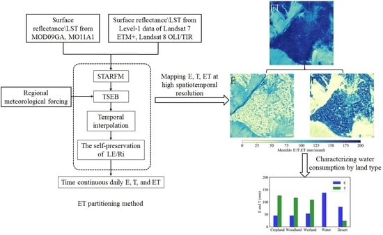
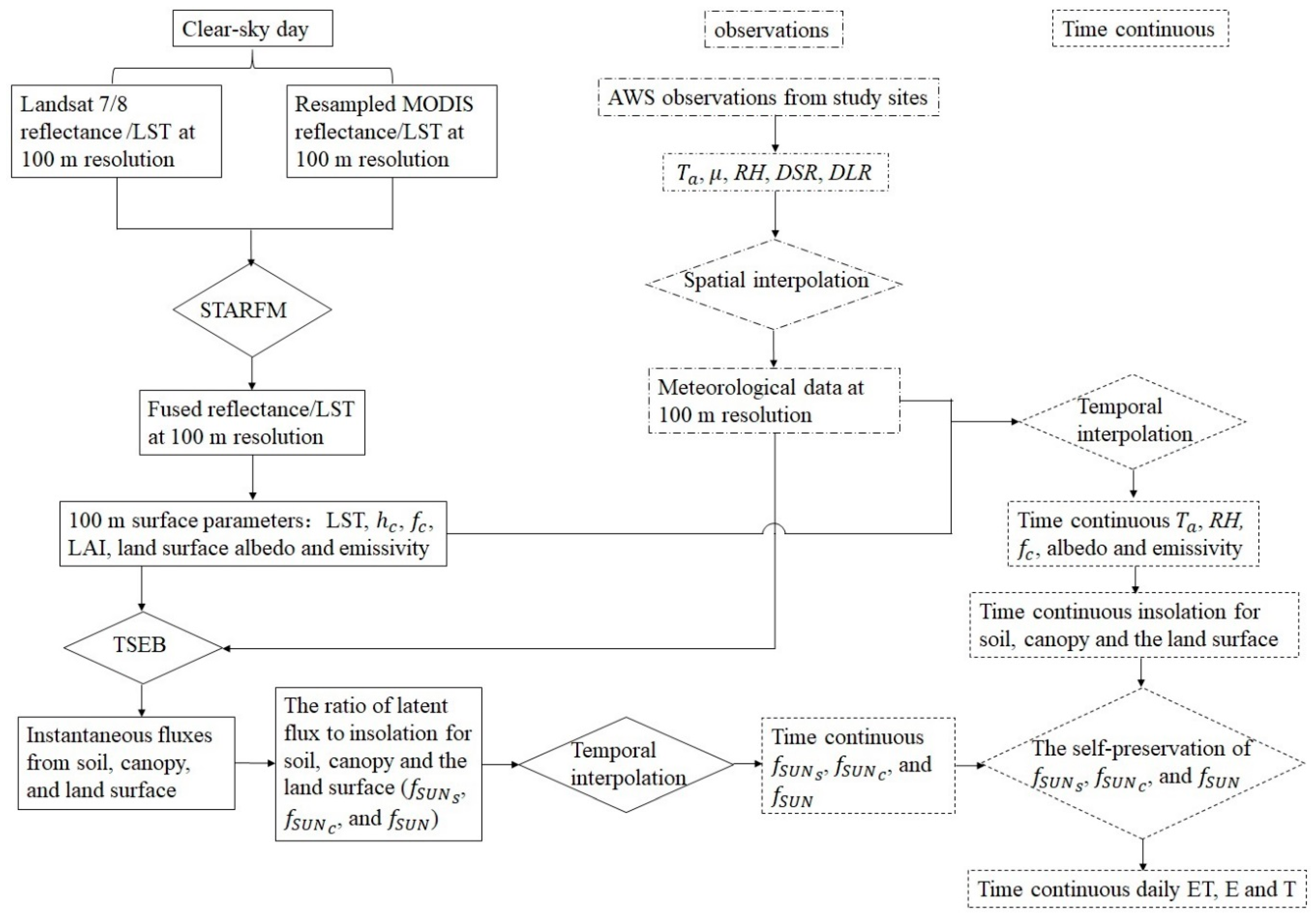
2.4. ET Partitioning Method

The ET partitioning method based on TSEB and multi-satellite data fusion is illustrated in Figure 2. For clear-sky days, the fused land surface reflectance at visible near infrared and shortwave bands and LST with MODIS temporal resolution and Landsat spatial resolution were derived based on STARFM. Then, the instantaneous land surface fluxes and the ratio of latent flux to insolation for soil ($f_{SUNs}$), canopy ($f_{SUNc}$), and composite land surface ($f_{SUN}$) were estimated based on TSEB by using land surface parameters calculated from fused data combined with regional meteorological inputs interpolated from observations. For cloudy days, the instantaneous $f_{SUNs}$, $f_{SUNc}$, and $f_{SUN}$ were obtained by linear interpolation based on an assumption that $f_{SUNs}$, $f_{SUNc}$, and $f_{SUN}$ changes linearly between the two adjacent clear days. Finally, the time continuous regional daily E, T, and ET were calculated based on the assumption of $f_{SUNs}$, $f_{SUNc}$, and $f_{SUN}$ is constant during the daylight hours [3].

2.5. TSEB Model

To estimate surface energy fluxes from soil and canopy components, Norman et al. [16] originally proposed the TSEB model, which has undergone several revisions [17,55,56,57,58,59] to accommodate more diverse land cover conditions. In TSEB, the surface energy balance for soil, canopy and the composite land surface are expressed as

$$R_{ns} = L{E}_s+H_s+G$$

(1)

$$R_{nc} = L{E}_c+H_c$$

(2)

$$R_n = LE+H+G$$

(3)

where $R_n$ is net radiation, $LE$ is latent heat flux, $H$ is sensible heat flux, $G$ is ground soil heat flux (all in W/m²). Subscript $s$ and $c$ represent soil and canopy components, respectively. Apart from $G$, all the land surface fluxes in Equation (3) can be calculated as the sum of soil and canopy components in Equation (1) and (2). $G$ is usually calculated as the fraction of $R_{ns}$ [16],

$$G = c_G{R}_{ns}$$

(4)

where $c_G$ is an empirical coefficients, which varies with time, soil type, and soil moisture. For satellite overpass time around solar noon, $c_G$ is assumed to be constant value of 0.35 for many soil type and moisture conditions [60].

The net radiation for soil ($R_{ns}$) and canopy ($R_{nc}$) are given as [17],

$$R_{ns} = {\tau }_{longwave}{L}_{\downarrow }+\left(1-{\tau }_{longwave}\right){\epsilon }_c\sigma T_c^4-{\epsilon }_s\sigma T_s^4+{\tau }_{solar}\left(1-{\alpha }_s\right)S_{\downarrow }$$

(5)

$$R_{nc} = \left(1-{\tau }_{longwave}\right)\left(L_{\downarrow }+{\epsilon }_s\sigma T_s^4-2{\epsilon }_c\sigma T_c^4-{\epsilon }_s\sigma T_s^4\right)+\left(1-{\tau }_{solar}\right)\left(1-{\alpha }_c\right)S_{\downarrow }$$

(6)

where $L_{\downarrow }$ and $S_{\downarrow }$ are incoming longwave and shortwave radiation (W/m²), respectively. ${\tau }_{longwave}$ and ${\tau }_{solar}$ are the transmittances of longwave and shortwave radiation through the canopy, respectively. $\epsilon$ and $\alpha$ are the emissivity and albedo, respectively. Subscript $s$ and $c$ represent soil and canopy components, respectively. $T_s$ and $T_c$ are soil and canopy components temperature (K), respectively.

By permitting the interaction between soil and canopy fluxes, Norman et al. [16] proposed a “series” version of TSEB, which is more robust to compute the sensible heat fluxes [61,62]. Following Norman et al. [16], $H$, $H_s$, and $H_c$ are expressed as

$$H = \rho C_P\frac{T_{ac}-T_a}{r_a}$$

(7)

$$H_s = \rho C_P\frac{T_s-T_{ac}}{r_s}$$

(8)

$$H_c = \rho C_P\frac{T_c-T_{ac}}{r_x}$$

(9)

where $\rho$ is the density of air (kg/m³), $C_P$ is the specific heat of air (J/(kg$·$K)), $T_{ac}$ is the air temperature in the canopy air layer (K), $T_a$ is the air temperature in the soil-canopy combined surface (K). $r_a$ is the bulk aerodynamic resistance (s/m), which is computed by using Monin–Obukhov surface layer similarity theory. The soil resistance $r_s$ (s/m) is derived according to Kustas and Norman [17]. $r_x$ is the boundary layer resistance of the canopy elements (s/m).

In TSEB, $T_s$ and $T_c$ in Equations (5), (6), (8), and (9) are related to satellite derived directional surface temperature ($T_R\left(\mathsf{\theta }\right)$) and the fraction vegetation cover ($f_c(\mathsf{\theta }$)), as expressed in [63],

$$T_R\left(\mathsf{\theta }\right)= {\left[f_c\left(\mathsf{\theta }\right)T_c^4+\left(1-f_c\left(\mathsf{\theta }\right)\right)T_s^4\right]}^{1/4}$$

(10)

where $\mathsf{\theta }$ is the view angle of thermal sensor. $T_s$ and $T_c$ can be calculated by iteration for Equations (2)–(10) with an initial value of $L{E}_c$, which is estimated based on Priestley–Taylor equation,

$$L{E}_c = {\alpha }_{PT}{f}_g\frac{∆}{∆+\gamma }{R}_{nc}$$

(11)

where $f_g$ is the fraction of $\mathrm{LAI}$ that is green, $∆$ is the slope of the saturation vapor pressure versus temperature curve (kPa/°C), $\gamma$ is the psychrometer constant (~0.066 kPa/°C). The ${\alpha }_{PT}$ term is the Priestley–Taylor parameter, which is assumed to be constant value of 1.26 for unstressed transpiring canopy. For stressed conditions which can cause $L{E}_s<0$, TSEB iteratively reduces the value of ${\alpha }_{PT}$ from 1.26 until $L{E}_s>0$ [63]. In addition, for the sparsely vegetated desert, the modification for initial value of $L{E}_c$ proposed by Zhuang and Wu [59] was adopted since it reduced bias between measured and modeled H. This modification was not as reliable in partitioning ET between E and T as the original TSEB for the cropland and therefore was not applied to this land cover type.

The instantaneous surface energy fluxes for soil, canopy, and composite land surface at MODIS overpass time are solved for iteratively with Equations (1)–(11) and are then upscaled to daily ET, E, and T based on the ratio of instantaneous to daily insolation approach [3,22,29,30,31],

$$f_{SUNi} = L{E}_i/R_{si}$$

(12)

$$L{E}_{id} = f_{SUNi}\times R_{sid}$$

(13)

where $R_{si}$ are instantaneous insolation. Subscript $i$ represents soil, canopy, or composite land surface. $L{E}_{id}$ and $R_{sid}$ are daily latent heat flux and insolation for soil, canopy, and composite land surface, respectively. Then $LE$, $L{E}_s$, and $L{E}_c$ are converted to daily ET, E, and T by dividing the latent heat of evaporation.

2.6. STARFM

The STARFM, originally proposed by Gao et al. [37] for fusing MODIS and Landsat surface reflectance, has been widely used to obtained high spatiotemporal information of LST [35,36], land use types [64], and ET [22,26,29,30,31,32,33]. In this study, STARFM was used to produce LST and land surface reflectance at spatial resolution of 100 m with temporal resolution of MODIS (hereinafter referred to as Landsat-like). When Landsat data are not available, the predicted Landsat-like data is determined by using existing Landsat/MODIS data pair/pairs based on a weighting function, which is developed using a moving search window method. In STARFM, the weighting function for central pixel of moving window can be expressed as

$$L\left(x_{w/2},y_{w/2},t_0\right) = {\displaystyle \sum }_{i = 1}^w{\displaystyle \sum }_{j = 1}^w{\displaystyle \sum }_{k = 1}^n{W}_{ijk}\times \left(M\left(x_i,y_j,t_0\right)+L\left(x_i,y_j,t_k\right)-M\left(x_i,y_j,t_k\right)\right)$$

(14)

where $L$ and $M$ denote the land surface reflectance/LST of Landsat and MODIS, respectively. $w$ is the size of searching window. $\left(x_{w/2},y_{w/2}\right)$ and $\left(x_i,y_i\right)$ are the location of central pixel and the neighboring pixel in searching window, respectively. The time variable $t_0$ and $t_k$ are the predication date and acquisition date of Landsat/MODIS data pair/pairs, respectively.$k$ is the number of Landsat/MODIS data pair/pairs. $W_{ijk}$ is the weight that represents the contribution of each neighboring pixel to the predicted central pixel. The weight $W_{ijk}$ is determined by spectral difference between MODIS and Landsat pair at $t_k$, temporal difference between MODIS data at $t_0$ and $t_k$, and the distance between central pixel and neighboring pixel. For more details of STARFM, please refer to Gao et al. [37].

2.7. Landsat-Only Interpolation

To evaluate the value added by MODIS in the fusion process, the daily ET estimated based on fused data and the daily ET estimated based on Landsat data using a simple Landsat-only interpolation scheme were compared with the observed daily ET from the EC flux, radiation and meteorological observations. The Landsat-only interpolation scheme has been widely used to obtain time continuous daily ET in Mapping Evapotranspiration with Internalized Calibration (METRIC) model based on the ratio of ET to reference ET ($f_{RET}$) [65],

$$f_{RET} = ET/E{T}_{ref}$$

(15)

where $E{T}_{ref}$ is the reference ET estimated based on the Penman–Monteith formulation of the Food and Agriculture Organization standard using meteorological data [66]. In this scheme, the time continuous $f_{RET}$ is determined by linear interpolation based on estimated $f_{RET}$ on Landsat overpass dates. Then, the time continuous daily ET is derived as the product of $f_{RET}$ and $E{T}_{ref}$.

3. Results

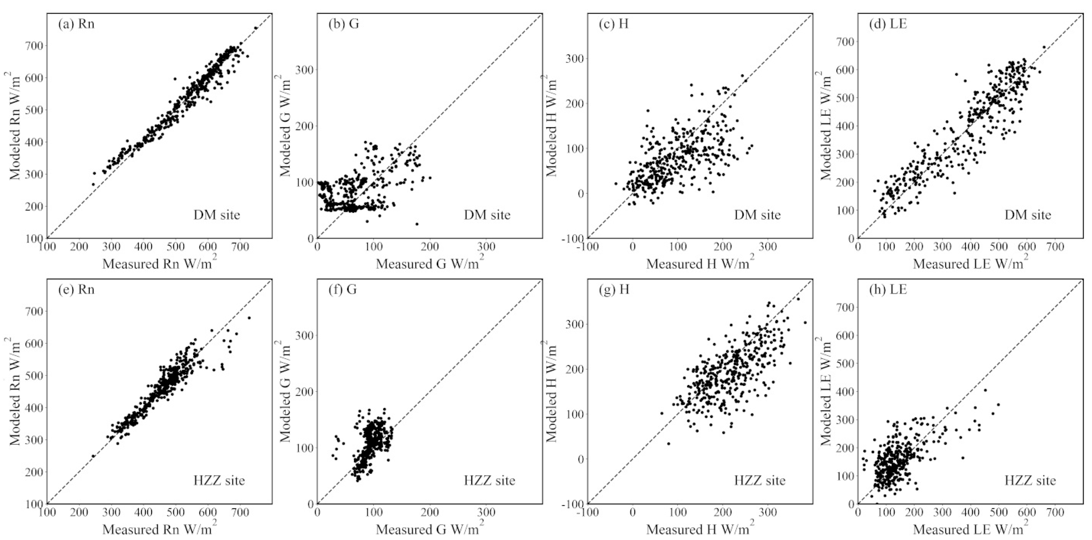
3.1. Evaluation of Land Surface Fluxes at The Study Sites

To assess the performance of the ET estimating method, the modeled and measured land surface fluxes including $R_n$, $G$, $H$, and $LE$ for the satellite overpass times were compared at the two study sites. For matching with the source areas of observations, the modeled land surface fluxes based on TSEB and fusion data were averaged over upwind source area (two pixels) at the two study sites [35,67]. The scatter plots in Figure 3 show the comparisons of modeled and measured land surface fluxes at DM and HZZ sites during 1 May to 31 October from 2012 to 2016. In addition, the statistical difference between measured and modeled land surface fluxes are given in

Table 2. The statistical difference of measured vs. modeled land surface fluxes at DM and HZZ sites during 1 May to 31 October from 2012 to 2016.

Study Site	Number	Error Type	Rn (W/m2)	G (W/m2)	H (W/m2)	LE (W/m2)
DM	391	Bias	2	12	−20	4
		RMSE	22	41	54	61
		MAPD	3%	47%	42%	12%
HZZ	395	Bias	1	13	−24	10
		RMSE	26	27	52	61
		MAPD	4%	22%	19%	32%

, including the bias error computed as the average difference between measured and modeled fluxes, the root mean square error (RMSE), and the mean absolute percent difference (MAPD).

From Figure 3 and Table 2, it appears that modeled $R_n$, $G$, $H$, and $LE$ agree well with the forced closure observations, with the scatter of points falling generally along the 1:1 line. RMSE values of ~25 W/m² for $R_n$, ~40 W/m² for $G$, ~55 W/m² for $H$, and ~60 W/m² for $LE$, indicate reasonable surface flux partitioning at both DM and HZZ sites. Compared with $G$, $H$, and $LE$, modeled $R_n$ has the best agreement with measured yielding a MAPD of 3% and 4% for DM site and HZZ site, respectively. The difference between modeled and measured $G$ is mainly caused by the considerable mismatch in source areas between soil heat flux plates (0.1–1 m) and the resolution of modeled fluxes (200 m) [68]. Compared with HZZ site covered by sparse vegetation, the modeled $G$ at DM site covered by irrigated maize with wider range of soil moisture and vegetation cover during the whole growing season, yields greater scatter with RMSE of 41 W/m² and MAPD of 47%, but shows a smaller bias of 12 W/m².

For $H$, the difference between modeled $H$ and observations from EC system illustrated in Figure 3c,g indicates a slightly underestimate with bias of −20 W/m² for DM site and −24 W/m² for HZZ site, which is consistent with the results from earlier studies [45,68]. For the residual of the surface energy balance $LE$, the values estimated using TSEB and fusion data yield good agreement with Bias of ~10 W/m² for both DM and HZZ sites when compared with flux tower observations using the residual-LE closure method. The MAPD value for $LE$ at DM site (12%) is less than the uncertainty of the EC measured $LE$ (18%) reported by Wang et al. [69]. However, the MAPD value is as larger as 32% at HZZ site due in part to the fact that the overall range in $LE$ values are relatively small under sparse arid vegetation cover and water-limited conditions.

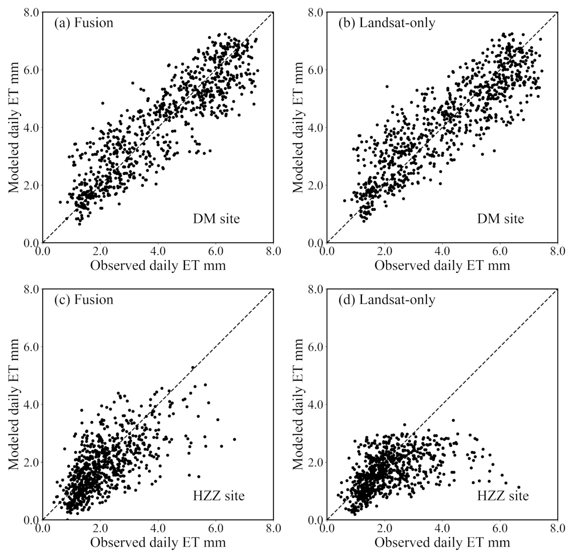
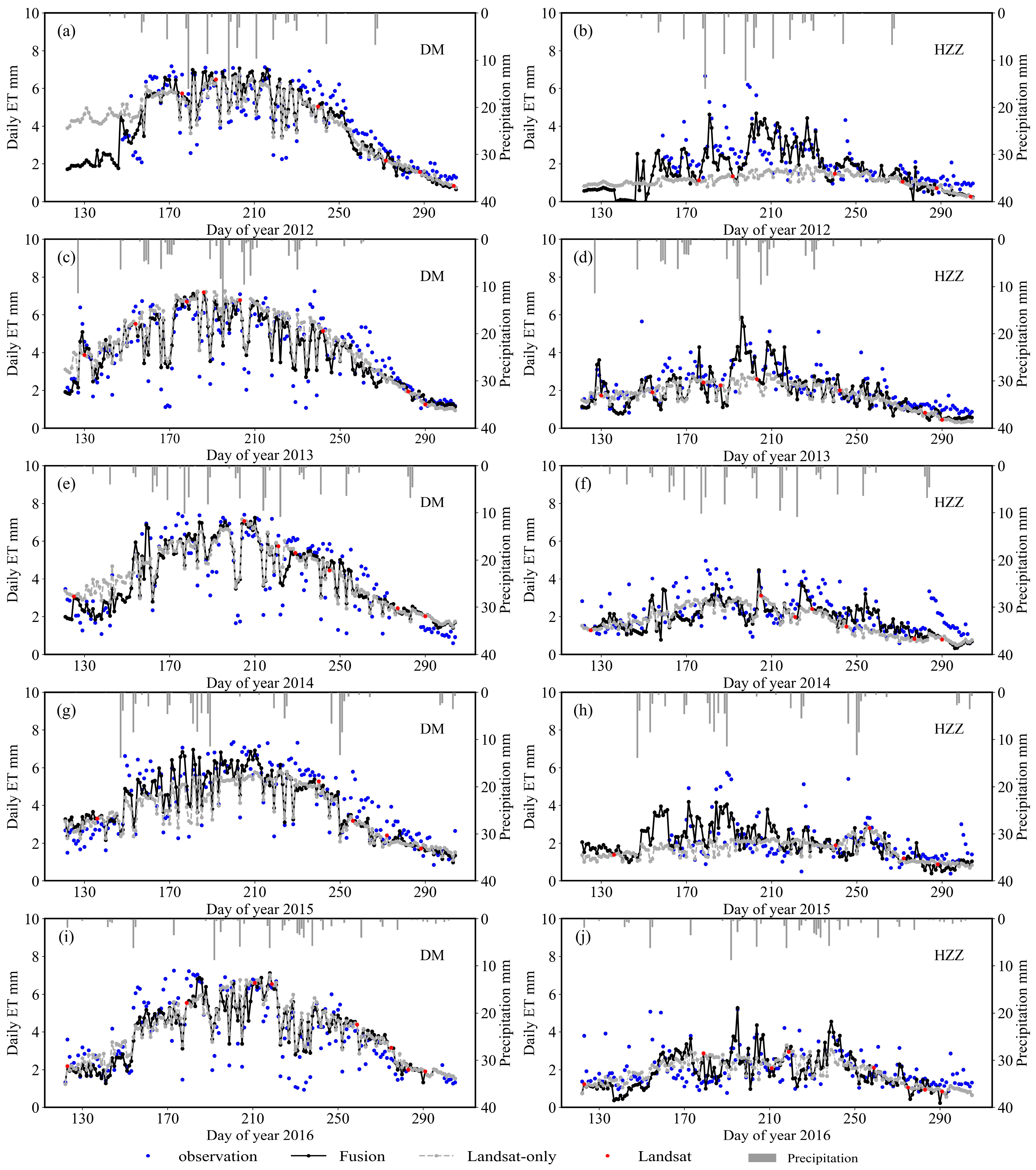
3.2. Evaluation of Daily ET at The Study Sites

To further evaluate the accuracy of the proposed ET estimating method as well as to assess the value added by MODIS in the fusion process, the modeled daily ET based on the proposed method and Landsat-only interpolation scheme were compared with the residual LE observations at the two flux tower sites (Figure 4). The error statistics for modeled daily ET based on both two methods are listed in

Table 3. The statistical results of observed daily ET vs. modeled daily ET based on TSEB and STARFM using fused data and modeled ET based on Landsat-only interpolation scheme at DM and HZZ sites for the period 1 May to 31 October from 2012 to 2016.

Study Site	Number	Error Type	Fusion	Landsat-Only
DM	825	Bias (mm)	0.01	0.04
		RMSE (mm)	0.85	0.91
		MAPD	16%	17%
HZZ	791	Bias(mm)	−0.25	−0.45
		RMSE (mm)	0.84	1.00
		MAPD	29%	33%

. Additionally, the time series of observed daily ET and modeled ET based on both two methods for the period 1 May to 31 October from 2012 to 2016 are shown in Figure 5.

For the DM site, the modeled daily ET using both methods agree well with observations, with similar scatter falling along the 1:1 line (Figure 4). The modeled daily ET using Landsat-only interpolation method show acceptable accuracy with bias, RMSE, and MAPD values of 0.04 mm, 0.91 mm, and 17%, respectively. By contrast, the modeled daily ET using TSEB and fusion data have slightly lower bias, RMSE and MAPD values of 0.01 mm, 0.85 mm, and 16%, indicating slightly better performance using this daily ET interpolation method. Given that there is sufficient irrigation and precipitation for the irrigated maize field to meet atmospheric demand at the DM site, the variation of ET is mainly affected by radiation. From Figure 5, we can see that the similar ET trends with low values correspond to decreased insolation on cloudy days were produced by the two daily ET interpolation methods during the whole study period. However, neither model captures the observed ET values falling below 3 mm. This is likely due to neither interpolation method providing accurate estimates under these low radiation conditions. Given that the lack of available Landsat data during DOY 125–170 in 2012 and 2014, and DOY 140–240 in 2015, the daily ET modeled from Landsat-only interpolation scheme differ greatly from both daily ET observed from EC and modeled from TSEB using the fusion data. This is an issue using Landsat-only interpolation, especially in regions with persistent cloud cover.

For HZZ site, better agreement between modeled and observed daily ET is achieved by using TSEB and data fusion. The modeled values of daily ET from the Landsat-only interpolation scheme are clearly underestimated when the observed values of daily ET are greater than 3 mm (Figure 4d). Daily ET modeled based on TSEB using fusion data yields bias, RMSE, and MAPD values of −0.25 mm, 0.84 mm, and 29%, respectively. By comparison, the underestimated daily ET based on Landsat-only interpolation scheme yields bias of −0.45 mm, RMSE of 1.00 mm, and MAPD of 33%. The HZZ site is located in a natural desert steppe with sparsely clumped vegetation and low soil moisture. As a result, the significant fluctuation of time series of daily ET is mainly caused by rainfall events. From Figure 5, it appears that the trend of daily ET modeled based on Landsat-only interpolation scheme is hard to capture the oscillations in ET caused by rainfall events, which significantly impacts soil evaporation and the subsequent rapid drying that again strongly impacts E. Since there is MODIS imagery often available soon after rainfall events, the more accurate temporal trend of daily ET is captured with relatively large ET increase after a rainfall event followed by drying of the soil surface, hence decreasing E and ET. Therefore, using TSEB and fusing MODIS and Landsat significantly improves daily ET over rainfed ecosystems, particularly with sparse vegetation cover where rapid changes in E significantly impact ET.

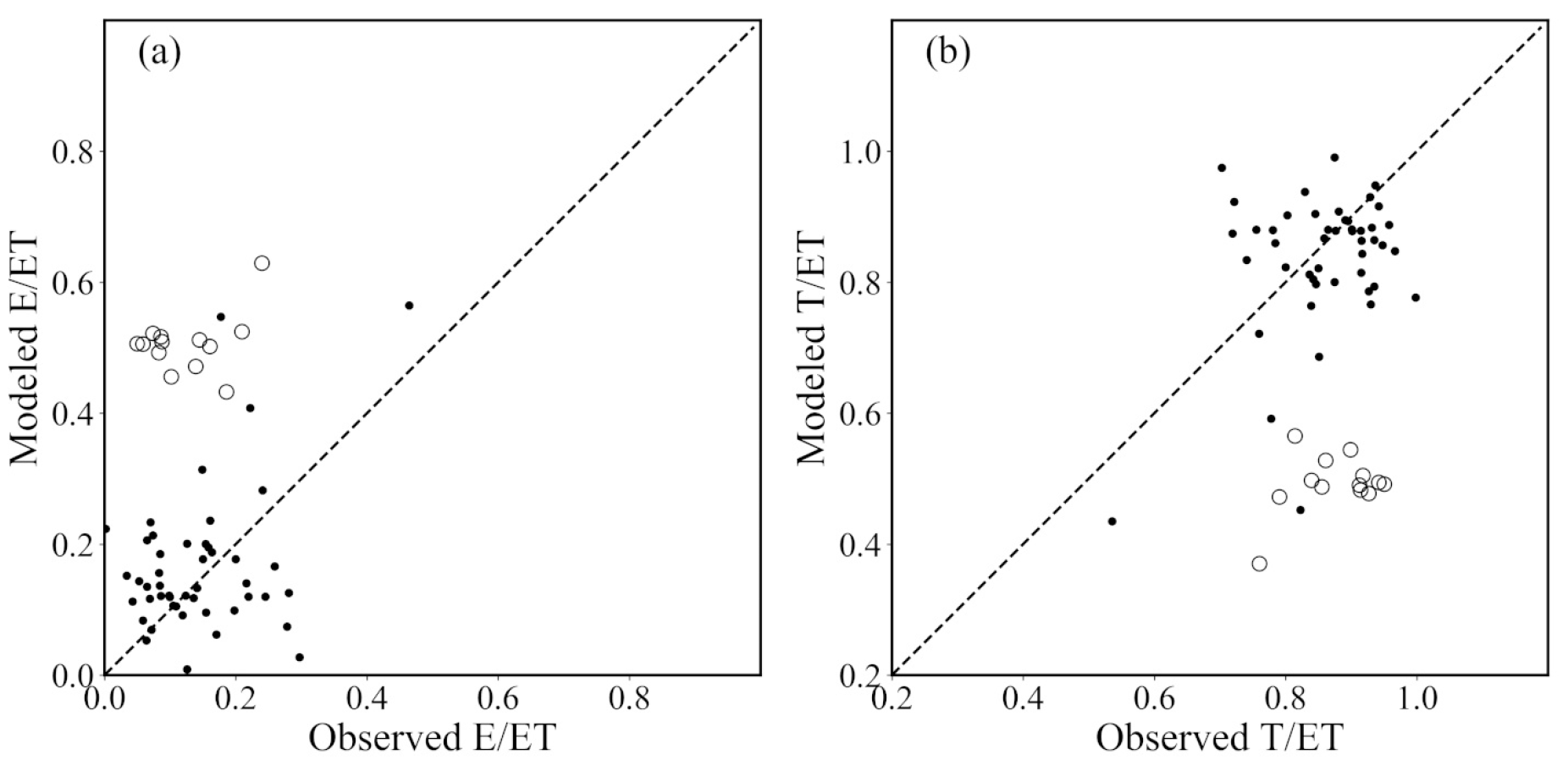
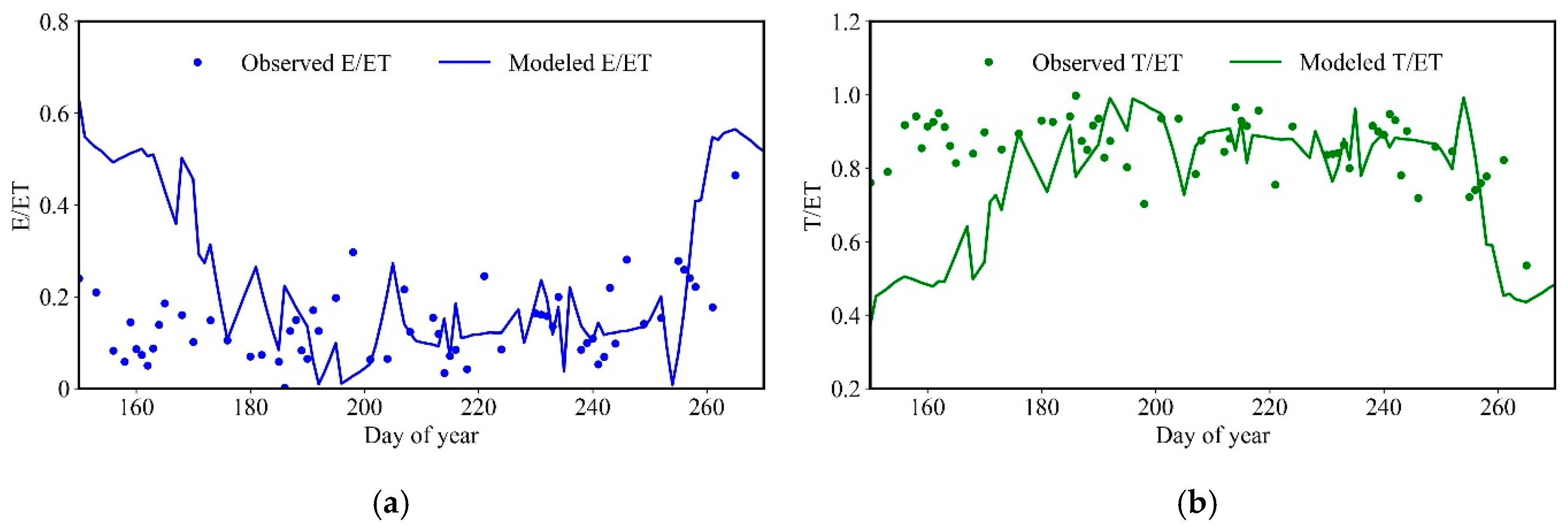
3.3. Evaluation of ET Partitioning Over The Cropland

The assessment of the ET partitioning method based on TSEB and fusion data was conducted by comparing with the ratios of E/ET and T/ET obtained from isotopic technology at DM site from 27 May (DOY 148) to 21 September (DOY 265) in 2012 [12], as illustrated in Figure 6 and

Table 4. The statistical results of observed E/ET and T/ET vs. modeled values for the period 27 May to 21 September, 2012 (DOY 148–265) at the DM site. The period where DOY >170 is when the plastic film has degraded from radiation and farm operations (see discussion below).

	Error Type	Overall (Number = 60)	DOY >170 (Number = 47)
E/ET	Bias	0.1	0
	RMSE	0.2	0.11
	MAPD	107%	53%
T/ET	Bias	−0.1	0
	RMSE	0.2	0.11
	MAPD	17%	10%

. For the period when the plastic film has deteriorated (DOY >170), the proposed method performs well for partitioning ET to E and T at the cropland site, with both values scattering around 1:1 line. However, outliers in E/ET and T/ET are under the early growing season when there is a plastic film significantly affecting the partitioning. For the whole growing season, this partitioning method based on TSEB and fusion data yields a bias of 0.1, a RMSE of 0.2, and a MAPD of 107% for E/ET while it produces a bias of −0.1, a RMSE of 0.2, and a MAPD of 17% for T/ET. The large MAPD value for E/ET is due to two factors: (1) the impact of the plastic film on E and T partitioning early in the growing season and (2) with most E/ET values below 0.3, any slight deviation in E/ET estimate significantly increases the value of the MAPD statistic.

The time series of observed and modeled E/ET and T/ET are illustrated in Figure 7. From Figure 7, it is confirmed that the large discrepancy between measured and modeled E/ET and T/ET for the group of points illustrated in Figure 6 occurs in the beginning of the growing season. As a previous study [23] concluded, this is due to the fact that the actual E/ET is reduced by the plastic film barrier deployed at the start of the growing season. This thin and disposal plastic film, covering approximately 60% of the soil surface, degrades from radiation and farming operations during the early growth stage of the maize. As a result, the plastic film is not an effective vapor barrier affecting observed E/ET and T/ET by the middle and later part of the growing season. The modeled E/ET and T/ET using TSEB and fusion data agree well with the observations in terms of both magnitude and temporal dynamics by the middle of the growing season. This suggests that the ET partitioning method predicted by TSEB can partition ET into E and T accurately over irrigated cropland as long as there are no artificial barriers reducing soil E. For the middle and late part of measurement period (DOY >170), the modeled E/ET from TSEB and fusion data yields bias, RMSE, and MAPD values of 0, 0.11, and 53%, respectively, and the modeled T/ET results in bias, RMSE, and MAPD values of 0, 0.11, and 10%, respectively.

4. Discussion

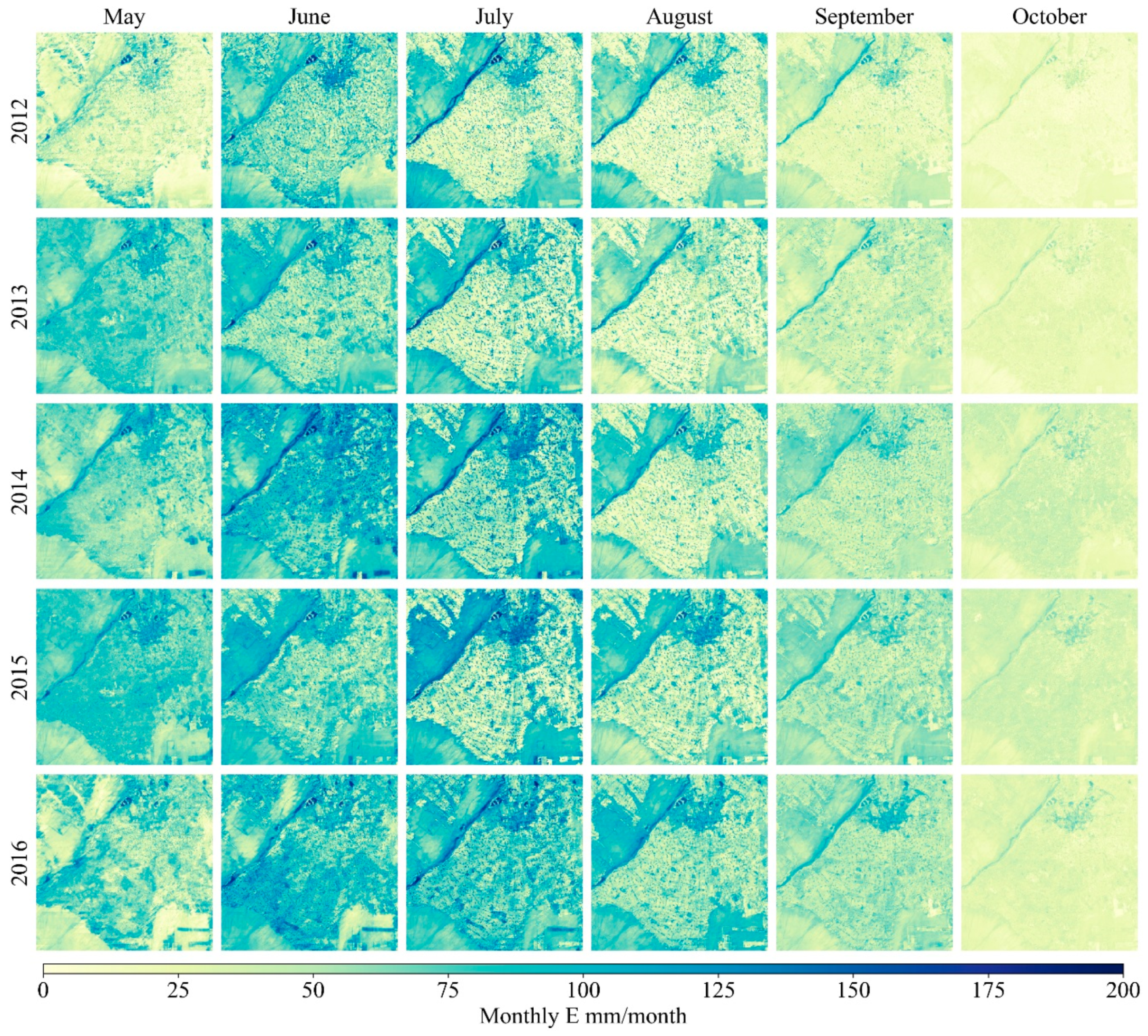
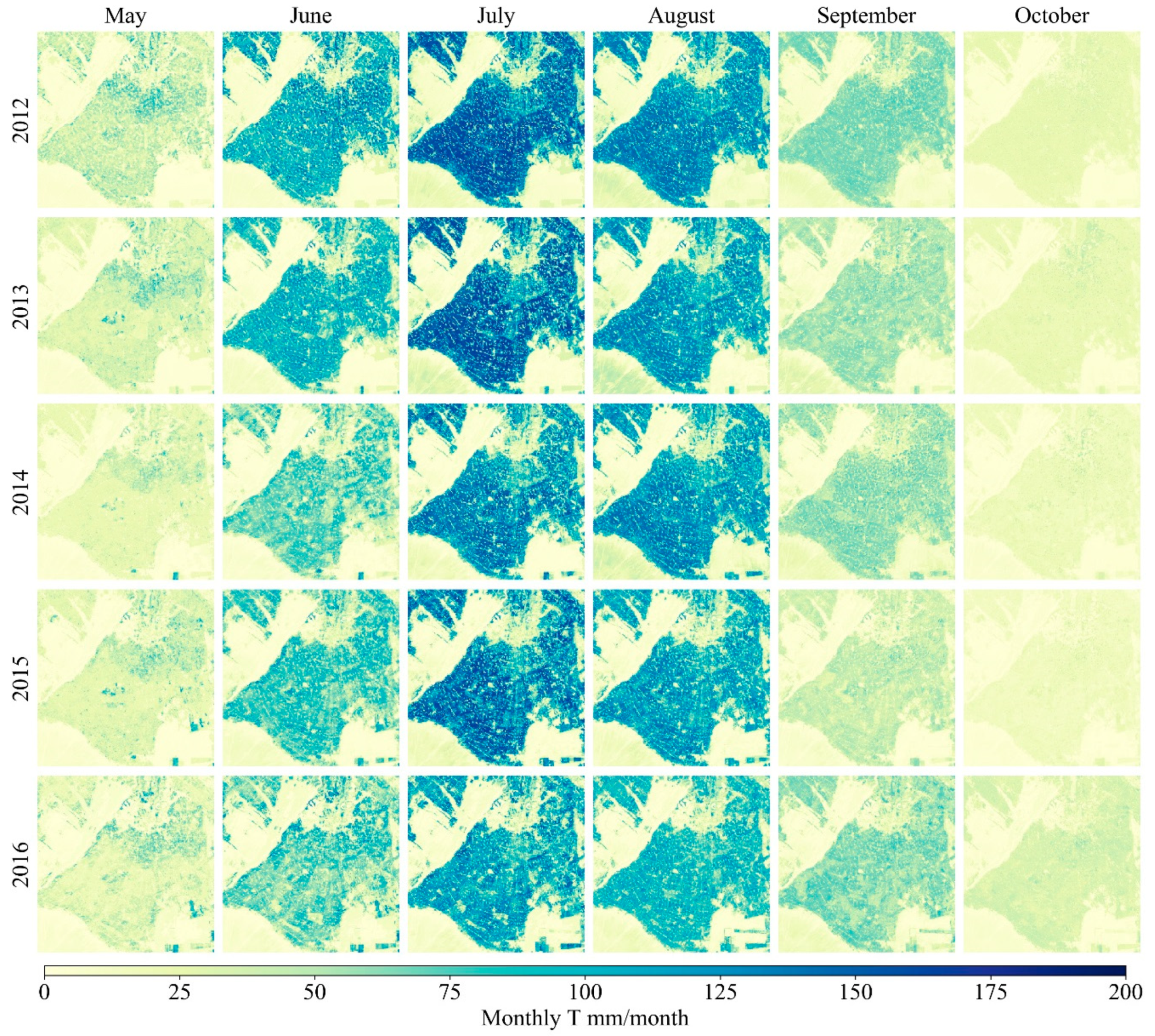
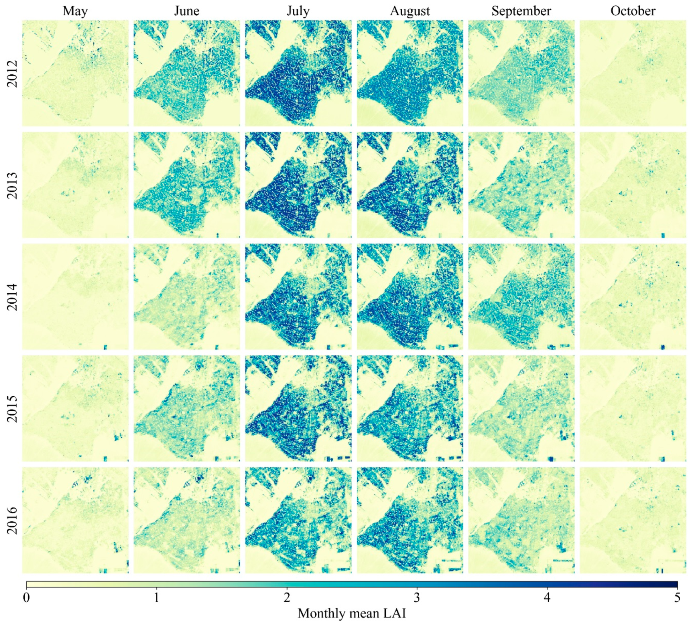
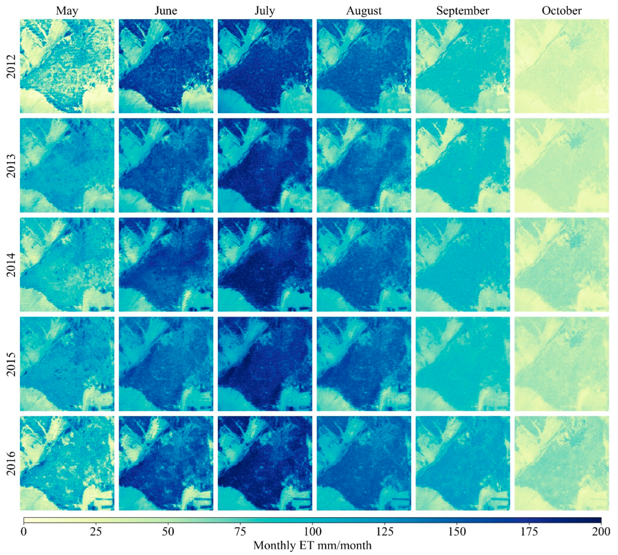
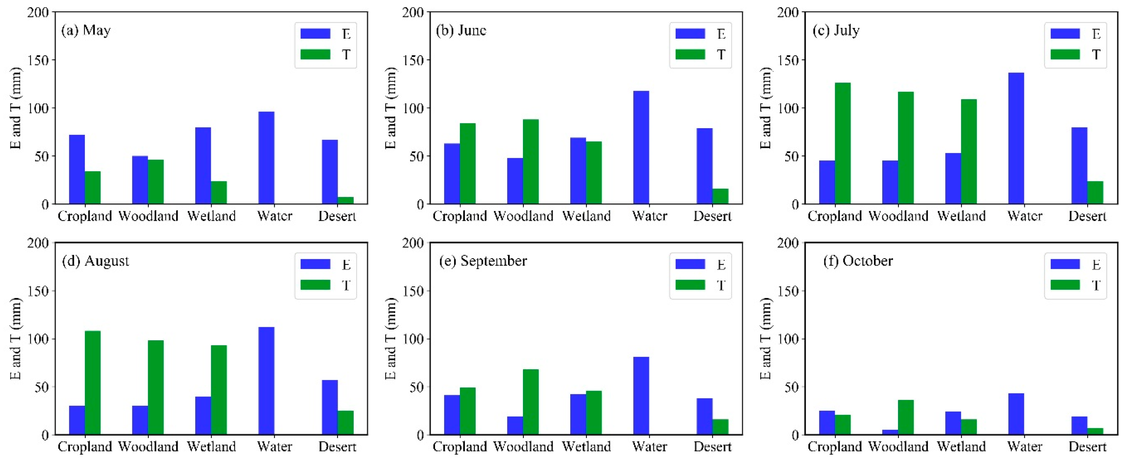
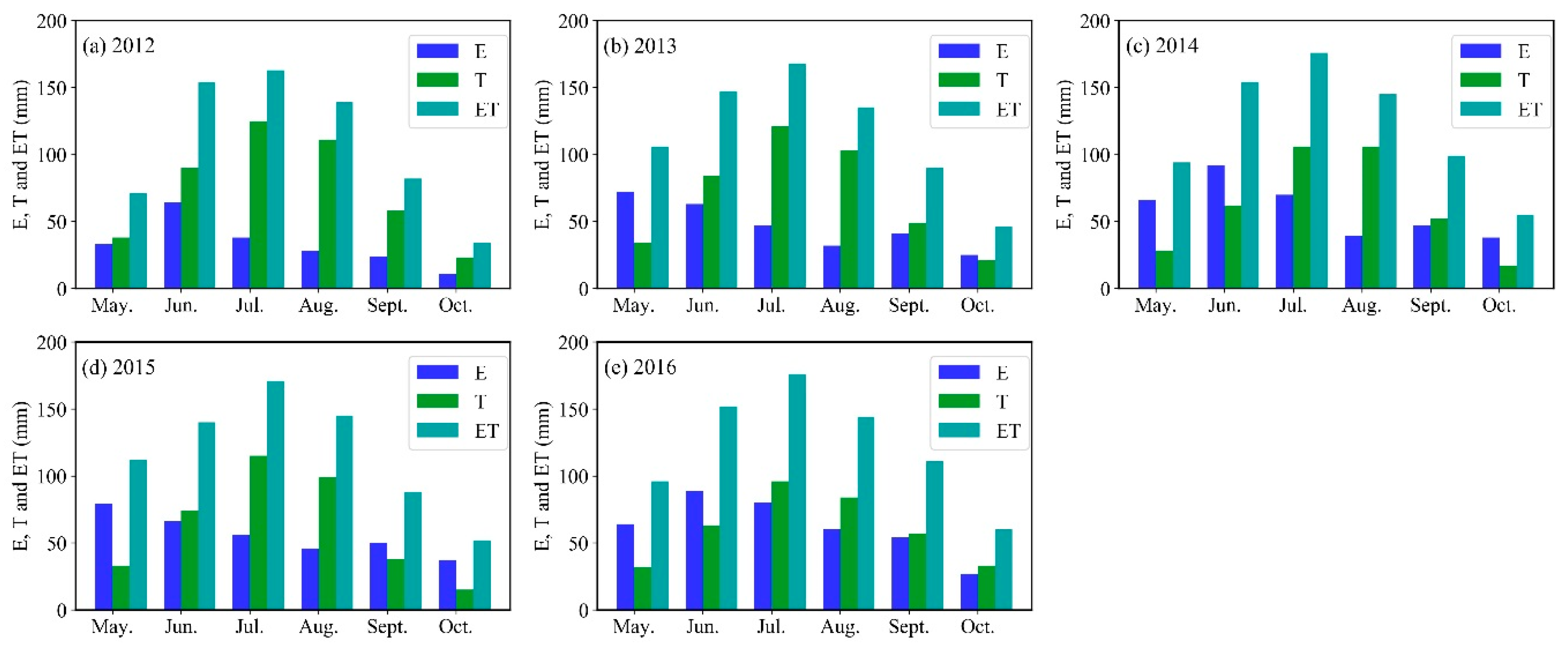
4.1. Spatiotemporal Patterns of E, T, and ET

Overall model validation in Section 3 indicates that the proposed ET partitioning method produced satisfactory estimates of ET and its partitioning, with statistical errors within the expected and reported errors in literature. The daily ET modeled based on TSEB using fusion data at study sites is comparable or had slightly better accuracy than previous studies [3,35,36,67,68]. The magnitude and temporal dynamics of modeled E/ET and T/ET in this study are consistent with results from model output based on the dual temperature difference (DTD) approach using MODIS data [3] and output from the two-source variational data assimilation (TVDA) system using in situ observations [23]. This indicates the current modeling approach incorporating data fusion can provide reliable E, T, and ET maps using Landsat and MODIS data.

The monthly E, T, and ET maps derived from modeled daily values from May to October from 2012 to 2016 in the study domain were produced for evaluating the E versus T as a function of land cover. From Figure 8, it appears that the seasonal variation and spatial diversity in monthly E fluctuates slightly from month to month and is affected by different land cover conditions. Given that the important factor influencing the magnitude of E—soil moisture, which is almost exclusively affected by the frequency of precipitation in rainfed environments [70], the monthly precipitation derived from averaged observation of two study sites is listed in

Table 5. Monthly precipitation (mm) during May to October from 2012 to 2016 in the study domain.

Years	May	June	July	August	September	October
2012	1.9	31.1	47.1	24.5	10.5	0.1
2013	18.5	33.0	58.9	17.9	3.0	0.0
2014	6.5	41.6	23.0	42.2	10.3	14.1
2015	18.2	31.2	30.4	12.0	33.1	9.4
2016	16.7	25.4	27.0	38.8	10.0	10.0

. For sparsely vegetated desert site, the seasonal fluctuation of monthly E coincides with that of precipitation illustrated in Table 5, due to the fact that the rate of E is correlated positively with soil moisture under water-limited condition [71,72]. The value of E for the desert site is relatively high in the middle of the summer season (i.e., from June to August) since the highest amount of precipitation normally occurs during this period, with a monthly mean precipitation of ~30 mm. On the other hand, precipitation is relatively low prior to June and after August with monthly mean precipitation of <15 mm.

The monthly E for the irrigated agricultural area (oasis) shows complex fluctuations during growing season that is influenced by solar irradiance, soil moisture, as well as vegetation cover. In the early part of growing season, the soil surface is partially covered by vegetation and soil moisture is relatively high due to the flood irrigation implemented once prior to the growing season and twice in the early growing season [23,73]. As a result, the rate of E in May and June is relatively high and fluctuates from year to year with changes in precipitation and timing of the irrigation. In the middle part of the growing season, the vegetation cover is relatively high, which rapidly reduces the amount of the solar irradiation and wind that reaches the soil surface both causing a significant reduction in E even if there are high soil moisture conditions. This results in the monthly E in July and August being smaller than that in May and June, even though the soil moisture is still relatively high due to frequent precipitation events and additional irrigation events. Compared to August, the rate of E in September is slightly increased mainly caused by the leaf senescence and harvesting crop that leads to the decrease of interception of solar irradiation and attenuation of wind. Lowest solar irradiation as well as relatively low soil moisture conditions due to low precipitation leads to the monthly E in October being the smallest during the study period.

The monthly T maps are illustrated in Figure 9. Considering that the seasonal variation trend of rate of T generally follows the temporal variability in LAI [3,5,72,73], the spatial pattern of monthly mean LAI derived from fusion data during the study period is shown in Figure 10. From Figure 9 and Figure 10, we can see that the seasonal variation, spatial variability, and differences in monthly T in different years is almost identical with the discrepancies in monthly mean LAI between different years. The spatio-temporal pattern for T distinguishes the oasis containing irrigated crops from the surrounding desert. During the whole growing season, the monthly T can be regarded as constant at about 20 mm for the desert vegetation and residential areas, while the T maps show seasonal variation for the oasis area where the value of T is driven by vegetation growth and biomass accumulation. The monthly T for oasis area increases from May to June with vegetation growth and reaches maximum in July with highest biomass accumulation of vegetation and then decreases from August to October associated with the leaf senescence.

As shown in Figure 11, the monthly ET, the sum of E and T, has significant seasonal variation over the six month period and spatial patterns for the different land cover types in the study domain. The ET values for cropland is clearly greater than surrounding desert during the whole growing season. Although the value of ET is dominated by rate of E for sparsely vegetated desert while dominated by rate of T for the irrigated croplands/oasis, the seasonal variation trend of ET in the oasis is similar to the surrounding desert. Comparison of ET maps in different years (cf. Figure 11), the trends in the seasonal variation in ET remain relatively consistent from 2012 to 2016. Naturally, the monthly ET in the middle growing season is larger than that in early and late growing season due to maximum plant biomass and precipitation/irrigation inputs. However, differences in amount and timing of the precipitation and irrigation events, plant growth rates and peak biomass differ from year to year. As a result, there are some apparent discrepancies in monthly cumulative ET for different years.

4.2. Water Consumption by Land Type

To characterize water consumption by different land covers in the study domain, the monthly value of E and T per unit area for cropland, woodland, wetland, water, and desert in 2013 are demonstrated in Figure 12. The densely vegetated area including cropland, woodland, and wetland significantly consume more water than the sparsely vegetated desert. The monthly E and T shows that there are differences in water loss from soil surface and water consumption for vegetation growth of densely vegetated land types caused by different soil moisture and phenology, growth, and development characteristics of the vegetation. The woodland consumes greatest amount of water for vegetation growth in early and late of growing season, while the cropland yielded the most plant water use in the middle of growing season.

The cropland, covering 53% of study area, consumes the greatest amount of surface water and groundwater for the study domain mainly from irrigation. To distinguish water consumption of the cropland for the years 2012 to 2016, the monthly E, T, and ET per unit area are illustrated in Figure 13. In general, the total water consumption of the cropland area remains relatively constant from 2012 to 2016 with cumulative ET ~675 mm during May to October but the water loss through evaporation from soil surface increases gradually, especially in July and August. The ratio of cumulative E to cumulative ET from May through October yields values of 0.31 for 2012, 0.41 for 2013, 0.47 for 2014, 0.46 for 2015, and 0.53 for 2016, respectively. With this increasing trend in E/ET, better irrigation strategies and water management decisions are urgently needed to reduce the water loss from the soil in the irrigated cropland area.

5. Conclusions

To provide detailed information of water use for agricultural water management at field and farm to landscape scales in semiarid and arid regions, a daily field-scale ET partitioning method developed by combining STARFM and TSEB was utilized and verified in the middle reaches of Heihe River Basin in this study. This method was developed by following the input parameter fusion scheme for estimating daily field-scale ET, which estimates ET, E, and T based on TSEB model formulations using land surface input parameters derived from data with spatiotemporal characteristics of MODIS and Landsat fused using STARFM.

In this study, daily ET, E, and T at spatial resolution of 100 m from May through October for the years 2012 to 2016 for the study area were estimated by using the ET partitioning method. A comparison of modeled instantaneous land surface fluxes and residual closure observations derived from the EC systems and AWSs at cropland and desert sites indicate that reliable surface fluxes were estimated using this method. In addition, the value added by incorporating MODIS in the fusion process for estimating daily ET, compared to Landsat-only interpolation scheme was assessed by comparing with ET observations for the irrigated cropland and desert sites. The results demonstrate that more accurate daily ET is produced by using the data fusion-based TSEB, with RMSE values of less than 1 mm/day for cropland and desert. We further tested the E and T partitioning capabilities of this proposed method for the cropland using E/ET and T/ET observed from isotopic technology. Apart from early growing season when the actual E was reduced by plastic film covering, the modeled E/ET and T/ET agreed well with observations in terms of both magnitude and temporal dynamics.

Maps of monthly E, T, and ET from May through October for the years 2012 to 2016 in the study area show reasonable temporal and spatial variability. The monthly E varies from month to month due to compounding effects from different land cover types being affected by precipitation, irrigation events and rate and amount of accumulated vegetation cover/biomass over the growing season. Meanwhile monthly T shows a consistent seasonal trend associated with vegetation growth and biomass production. Moreover, water consumption by different land cover types was conducted based on spatiotemporal distributions of E and T, reflecting the influence of soil moisture, fractional vegetation cover and phenology on E and T partitioning. The general relative increase in water loss through evaporation from bare soil in irrigated cropland during the growing season from 2012 to 2016 indicates that irrigation and water management strategies are urgently needed for conserving water resources in the Heihe River Basin.

As far as modeling the effect of plastic film layers for reducing E, previous studies indicate that the accuracy in estimating ET and its partitioning using Priestly–Taylor [74] and Shuttleworth–Wallace [75] modeling approaches with plastic film-mulching can be improved by incorporating the effect of mulching fraction on E. Based on these previous studies, we plan to develop and evaluate a refinement in the TSEB algorithm for computing E for fields containing plastic films. Due to the limitation of observations of ET partitioning into E and T, model validation could only be conducted for the oasis–desert ecosystem. Future plans include verifying the utility of this ET partitioning method over a wider range of land cover types using eddy covariance-based techniques [13,14].

References

1. Kirda, C.; Kanber, R. Water, no longer a plentiful resource, should be used sparingly in irrigated agriculture. In Crop Yield Response to Deficit Irrigation; Kluwer Academic Publishers: Dordrecht, The Netherlands, 1999; pp. 1–20. [Google Scholar]
2. Fernández, J.E.; Slawinski, C.; Moreno, F.; Walczak, R.T.; Vanclooster, M. Simulating the fate of water in a soil–crop system of a semi-arid Mediterranean area with the wave 2.1 and the euro-access-ii models. Agric. Water Manag. 2002, 56, 113–129. [Google Scholar] [CrossRef]
3. Song, L.S.; Liu, S.M.; Kustas, W.P.; Nieto, H.; Sun, L.; Xu, Z.W.; Skaggs, T.H.; Yang, Y.; Ma, M.G.; Xu, T.R.; et al. Monitoring and validating spatially and temporally continuous daily evaporation and transpiration at river basin scale. Remote Sens. Environ. 2018, 219, 72–88. [Google Scholar] [CrossRef]
4. Kool, D.; Agam, N.; Lazarovitch, N.; Heitman, J.L.; Sauer, T.J.; Ben-Gal, A. A review of approaches for evapotranspiration partitioning. Agric. For. Meteorol. 2014, 184, 56–70. [Google Scholar] [CrossRef]
5. Kustas, W.P.; Alfieri, J.G.; Nieto, H.; Wilson, T.G.; Gao, F.; Anderson, M.C. Utility of the two-source energy balance (TSEB) model in vine and interrow flux partitioning over the growing season. Irrig. Sci. 2019, 37, 375–388. [Google Scholar] [CrossRef]
6. Moran, M.S. Thermal infrared measurement as an indicator of plant ecosystem health. In Thermal Remote Sensing in Land Surface Processes; CRC press: Boca Raton, FL, USA, 2004; pp. 257–282. [Google Scholar]
7. Semmens, K.A.; Anderson, M.C.; Kustas, W.P.; Gao, F.; Alfieri, J.G.; McKee, L.; Prueger, J.H.; Hain, C.R.; Cammalleri, C.; Yang, Y.; et al. Monitoring daily evapotranspiration over two California vineyards using landsat 8 in a multi-sensor data fusion approach. Remote Sens. Environ. 2016, 185, 155–170. [Google Scholar] [CrossRef] [Green Version]
8. Courault, D.; Seguin, B.; Olioso, A. Review on estimation of evapotranspiration from remote sensing data: From empirical to numerical modeling approaches. Irrig. Drain. Syst. 2005, 19, 223–249. [Google Scholar] [CrossRef]
9. Kalma, J.D.; Mcvicar, T.R.; Mccabe, M.F. Estimating land surface evaporation: A review of methods using remotely sensed surface temperature data. Surv. Geophys. 2008, 29, 421–469. [Google Scholar] [CrossRef]
10. Wang, K.C.; Dickinson, R.E. A review of global terrestrial evapotranspiration: Observation, modeling, climatology, and climatic variability. Rev. Geophys. 2012, 50. [Google Scholar] [CrossRef]
11. Qiao, C.; Sun, R.; Xu, Z.W.; Zhang, L.; Liu, L.Y.; Hao, L.Y.; Jiang, G.Q. A study of shelterbelt transpiration and cropland evapotranspiration in an irrigated area in the middle reaches of the Heihe river in northwestern china. IEEE Geosci. Remote Sens. Lett. 2015, 12, 369–373. [Google Scholar] [CrossRef]
12. Wen, X.F.; Yang, B.; Sun, X.M.; Lee, X.H. Evapotranspiration partitioning through in-situ Oxygen isotope measurements in an oasis cropland. Agric. For. Meteorol. 2016, 230–231, 89–96. [Google Scholar] [CrossRef] [Green Version]
13. Scanlon, T.M.; Kustas, W.P. Partitioning evapotranspiration using an eddy covariance-based technique: Improved assessment of soil moisture and land–atmosphere exchange dynamics. Vadose Zone J. 2012, 11, 1–7. [Google Scholar] [CrossRef]
14. Scanlon, T.M.; Schmidt, D.F.; Skaggs, T.H. Correlation-based flux partitioning of water vapor and carbon dioxide fluxes: Method simplification and estimation of canopy water use efficiency. Agric. For. Meteorol. 2019, 279, 107732. [Google Scholar] [CrossRef]
15. Talsma, C.J.; Good, S.P.; Carlos, J.; Brecht, M.; Fisher, J.B.; Miralles, D.G.; McCabe, M.; Purdy, A.J. Partitioning of evapotranspiration in remote sensing-based models. Agric. For. Meteorol. 2018, 260–261, 131–143. [Google Scholar] [CrossRef]
16. Norman, J.M.; Kustas, W.P.; Humes, K.S. Source approach for estimating soil and vegetation energy fluxes in observations of directional radiometric surface temperature. Agric. For. Meteorol. 1995, 77, 263–293. [Google Scholar] [CrossRef]
17. Kustas, W.P.; Norman, J.M. Evaluation of soil and vegetation heat flux predictions using a simple two-source model with radiometric temperatures for partial canopy cover. Agric. For. Meteorol. 1999, 94, 13–29. [Google Scholar] [CrossRef]
18. Fisher, J.B.; Tu, K.P.; Baldocchi, D.D. Global estimates of the land–atmosphere water flux based on monthly AVHRR and ISLSCP-II data, validated at 16 FLUXNETsites. Remote Sens. Environ. 2008, 112, 901–919. [Google Scholar] [CrossRef]
19. Miralles, D.G.; Gash, J.H.; Holmes, T.R.H.; Jeu, R.A.M.D.; Dolman, A.J. Global canopy interception from satellite observations. J. Geophys. Res. Atmos. 2010, 115, D16122. [Google Scholar] [CrossRef]
20. Mu, Q.Z.; Zhao, M.S.; Running, S.W. Improvements to a MODIS global terrestrial evapotranspiration algorithm. Remote Sens. Environ. 2011, 115, 1781–1800. [Google Scholar] [CrossRef]
21. Bellvert, J.; Jofre-Cekalovic, C.; Pelecha, A.; Mata, M.; Nieto, H. Feasibility of using the two-source energy balance model (TSEB) with Sentinel-2 and Sentinel-3 images to analyze the spatio-temporal variability of vine water status in a vineyard. Remote Sens. 2020, 12, 2229. [Google Scholar] [CrossRef]
22. Sun, L.; Anderson, M.C.; Gao, F.; Hain, C.; Alfieri, J.G.; Sharifi, A.; McCarty, G.W.; Yang, Y.; Yang, Y.; Kustas, W.P.; et al. Investigating water use over the Choptank river watershed using a multisatellite data fusion approach. Water Resour. Res. 2017, 53, 5298–5319. [Google Scholar] [CrossRef] [Green Version]
23. Xu, T.R.; Bateni, S.; Margulis, S.; Song, L.S.; Liu, S.M.; Xu, Z.W. Partitioning evapotranspiration into soil evaporation and canopy transpiration via a two-source variational data assimilation system. J. Hydrometeorol. 2016, 17, 2353–2370. [Google Scholar] [CrossRef]
24. Yao, Y.J.; Liang, S.L.; Yu, J.; Chen, J.Q.; Liu, S.M.; Lin, Y.; Fisher, J.B.; McVicar, T.R.; Cheng, J.; Jia, K.; et al. A simple temperature domain two-source model for estimating agricultural field surface energy fluxes from Landsat images. J. Geophys. Res. Atmos. 2017, 122, 5211–5236. [Google Scholar] [CrossRef]
25. Cammalleri, C.; Anderson, M.C.; Gao, F.; Hain, C.R.; Kustas, W.P. A data fusion approach for mapping daily evapotranspiration at field scale. Water Resour. Res. 2013, 49, 4672–4686. [Google Scholar] [CrossRef]
26. Anderson, M.C.; Kustas, W.P.; Norman, J.M.; Hain, C.R.; Mecikalski, J.R.; Schultz, L.; Gonzalez-Dugo, M.P.; Cammalleri, C.; d’Urso, G.; Pimstein, A.; et al. Mapping daily evapotranspiration at field to continental scales using geostationary and polar orbiting satellite imagery. Hydrol. Earth Syst. Sci. 2011, 15, 223–239. [Google Scholar] [CrossRef] [Green Version]
27. Kustas, W.P.; Norman, J.M.; Anderson, M.C.; French, A.N. Estimating subpixel surface temperatures and energy fluxes from the vegetation index–radiometric temperature relationship. Remote Sens. Environ. 2003, 85, 429–440. [Google Scholar] [CrossRef]
28. Bai, L.L.; Cai, J.B.; Liu, Y.; Chen, H.; Zhang, B.Z.; Huang, L.X. Responses of field evapotranspiration to the changes of cropping pattern and groundwater depth in large irrigation district of Yellow river basin. Agric. Water Manag. 2017, 188, 1–11. [Google Scholar] [CrossRef]
29. Cammalleri, C.; Anderson, M.C.; Gao, F.; Hain, C.R.; Kustas, W.P. Mapping daily evapotranspiration at field scales over rainfed and irrigated agricultural areas using remote sensing data fusion. Agric. For. Meteorol. 2014, 186, 1–11. [Google Scholar] [CrossRef] [Green Version]
30. Knipper, K.R.; Kustas, W.P.; Anderson, M.C.; Alfieri, J.G.; Prueger, J.H.; Hain, C.R.; Gao, F.; Yang, Y.; Mckee, L.G.; Nieto, H.; et al. Evapotranspiration estimates derived using thermal-based satellite remote sensing and data fusion for irrigation management in California vineyards. Irrig. Sci. 2019, 37, 431–449. [Google Scholar] [CrossRef]
31. Yang, Y.; Anderson, M.C.; Gao, F.; Hain, C.; Noormets, A.; Sun, G.; Wynne, R.; Thomas, V.; Sun, L. Investigating impacts of drought and disturbance on evapotranspiration over a forested landscape in North Carolina, USA using high spatiotemporal resolution remotely sensed data. Remote Sens. Environ. 2020, 238, 111018. [Google Scholar] [CrossRef]
32. Yang, Y.; Anderson, M.C.; Gao, F.; Hain, C.R.; Semmens, K.A.; Kustas, W.P.; Noormets, A.; Wynne, R.H.; Thomas, V.A.; Sun, G. Daily Landsat-scale evapotranspiration estimation over a forested landscape in North CarolinaUSA, using multi-satellite data fusion. Hydrol. Earth Syst. Sci 2017, 21, 1017–1037. [Google Scholar] [CrossRef] [Green Version]
33. Yang, Y.; Anderson, M.C.; Gao, F.; Wardlow, B.; Hain, C.R.; Otkin, J.A.; Alfieri, J.; Yang, Y.; Sun, L.; Dulaney, W. Field-scale mapping of evaporative stress indicators of crop yield: An application over mead, NE, USA. Remote Sens. Environ. 2018, 210, 387–402. [Google Scholar] [CrossRef]
34. Guzinski, R.; Nieto, H. Evaluating the feasibility of using Sentinel-2 and Sentinel-3 satellites for high-resolution evapotranspiration estimations. Remote Sens. Environ. 2019, 221, 157–172. [Google Scholar] [CrossRef]
35. Li, Y.; Huang, C.L.; Hou, J.L.; Gu, J.; Zhu, G.F.; Li, X. Mapping daily evapotranspiration based on spatiotemporal fusion of ASTER and MODIS images over irrigated agricultural areas in the Heihe River Basin, Northwest China. Agric. For. Meteorol. 2017, 244, 82–97. [Google Scholar] [CrossRef]
36. Ma, Y.F.; Liu, S.M.; Song, L.S.; Xu, Z.W.; Liu, Y.L.; Xu, T.R.; Zhu, Z.L. Estimation of daily evapotranspiration and irrigation water efficiency at a landsat-like scale for an arid irrigation area using multi-source remote sensing data. Remote Sens. Environ. 2018, 216, 715–734. [Google Scholar] [CrossRef]
37. Gao, F.; Masek, J.; Schwaller, M.; Hall, F. On the blending of the Landsat and MODIS surface reflectance: Predicting daily Landsat surface reflectance. IEEE Trans. Geosci. Remote Sens. 2006, 44, 2207–2218. [Google Scholar]
38. Cheng, G.D.; Li, X.; Zhao, W.Z.; Xu, Z.M.; Feng, Q.; Xiao, S.C.; Xiao, H.L. Integrated study of the water-ecosystem-economy in the Heihe River Basin. Natl. Sci. Rev. 2014, 1, 413–428. [Google Scholar] [CrossRef] [Green Version]
39. Li, X.; Cheng, G.D.; Ge, Y.C.; Li, H.Y.; Han, F.; Hu, X.L.; Tian, W.; Tian, Y.; Pan, X.D.; Nian, Y.Y.; et al. Hydrological cycle in the heihe river basin and its implication for water resource management in endorheic basins. J. Geophys. Res. Atmos. 2018, 123, 890–914. [Google Scholar] [CrossRef]
40. Li, X.; Cheng, G.D.; Liu, S.M.; Xiao, Q.; Ma, M.M.; Jin, R.; Che, T.; Liu, Q.H.; Wang, W.Z.; Qi, Y.; et al. Heihe watershed allied telemetry experimental research (HiWATER): Scientific objectives and experimental design. Bull. Am. Meteorol. Soc. 2013, 94, 1145–1160. [Google Scholar] [CrossRef]
41. Liu, S.M.; Li, X.; Xu, Z.W.; Che, T.; Xiao, Q.; Ma, M.G.; Liu, Q.H.; Jin, R.; Guo, J.W.; Wang, L.X.; et al. The Heihe integrated observatory network: A basin-scale land surface processes observatory in China. Vadose Zone J. 2018, 17, 180072. [Google Scholar] [CrossRef]
42. Liu, S.M.; Xu, Z.W.; Song, L.S.; Zhao, Q.Y.; Ge, Y.; Xu, T.R.; Ma, Y.F.; Zhu, Z.L.; Jia, Z.Z.; Zhang, F. Upscaling evapotranspiration measurements from multi-site to the satellite pixel scale over heterogeneous land surfaces. Agric. For. Meteorol. 2016, 230–231, 97–113. [Google Scholar] [CrossRef]
43. Liu, S.M.; Xu, Z.W.; Wang, W.Z.; Jia, Z.Z.; Zhu, M.J.; Bai, J.W.; Wang, J.M. A comparison of eddy-covariance and large aperture scintillometer measurements with respect to the energy balance closure problem. Hydrol. Earth Syst. Sci. 2011, 15, 1291–1306. [Google Scholar] [CrossRef] [Green Version]
44. Xu, Z.W.; Liu, S.M.; Li, X.; Shi, S.J.; Wang, J.M.; Zhu, Z.L.; Xu, T.R.; Wang, W.Z.; Ma, M.G. Intercomparison of surface energy flux measurement systems used during the HiWATER-MUSOEXE. J. Geophys. Res. Atmos. 2013, 118, 13140–13157. [Google Scholar] [CrossRef]
45. Li, Y.; Kustas, W.P.; Huang, C.L.; Nieto, H.; Haghighi, E.; Anderson, M.C.; Domingo, F.; Garcia, M.; Scott, L.R. Evaluating soil resistance formulations in thermal-based two-source energy balance (TSEB) model: Implications for heterogeneous semiarid and arid regions. Water Resour. Res. 2019, 55, 1059–1078. [Google Scholar] [CrossRef] [Green Version]
46. Yang, K.; Wang, J.M. A temperature prediction-correction method for estimating surface soil heat flux from soil temperature and moisture data. Sci. China Ser. Earth Sci. 2008, 51, 721–729. [Google Scholar] [CrossRef]
47. Prueger, J.H.; Hatfield, J.L.; Kustas, W.P.; Hipps, L.E.; MacPherson, J.I.; Neale, C.M.U.; Eichinger, W.E.; Cooper, D.I.; Parkin, T.B. Tower and aircraft Eddy Covariance measurements of water vapor, energy, and carbon dioxide fluxes during SMACEX. J. Hydrometeorol. 2005, 6, 954–960. [Google Scholar] [CrossRef]
48. Twine, T.E.; Kustas, W.P.; Norman, J.M.; Cook, D.R.; Houser, P.R.; Mayers, T.P.; Prueger, J.H.; Starks, P.J.; Wesely, M.L. Correcting eddy covariance flux underestimation over a grassland. Agric. For. Meteorol. 2000, 103, 279–300. [Google Scholar] [CrossRef] [Green Version]
49. Sun, L.; Chen, Z.X.; Gao, F.; Anderson, M.C.; Song, L.S.; Wang, L.M.; Hu, B.; Yang, Y. Reconstructing daily clear-sky land surface temperature for cloudy regions from Modis data. Comput. Geosci. 2017, 105, 10–20. [Google Scholar] [CrossRef]
50. Scaramuzza, P.; Micijevic, E.; Chander, G. SLC Gap-Filled Products Phase One Methodology. 2004. Available online: https://landsat.usgs.gov/sites/default/files/documents/SLC_Gap_Fill_Methodology.pdf (accessed on 28 May 2009).
51. Yu, X.; Guo, X.; Wu, Z. Land surface temperature retrieval from landsat 8 tirs-comparison between radiative transfer equation-based method, split window algorithm and single channel method. Remote Sens. 2014, 6, 9829–9852. [Google Scholar] [CrossRef] [Green Version]
52. Gutman, G.; Ignatov, A. The derivation of the green vegetation fraction from NOAA/AVHRR data for use in numerical weather prediction models. Int. J. Remote Sens 1998, 19, 1533–1543. [Google Scholar] [CrossRef]
53. Choudhury, B.J. Relationships between vegetation indices, radiation absorption, and net photosynthesis evaluated by a sensitivity analysis. Remote Sens. Environ. 1987, 22, 209–233. [Google Scholar] [CrossRef]
54. Zhong, B.; Yang, A.X.; Nie, A.H.; Yao, Y.J.; Zhang, H.; Wu, S.L.; Liu, Q.H. Finer resolution land-cover mapping using multiple classifiers and multisource remotely sensed data in the Heihe River Basin. IEEE J. Sel. Top. Appl. Earth Obs. Remote Sens. 2015, 99, 1–20. [Google Scholar] [CrossRef]
55. Campbell, G.S.; Norman, J.M. An Introduction to Environmental Biophysics; Springer Science and Business Media: New York, NY, USA, 1998; p. 286. [Google Scholar]
56. Colaizzi, P.D.; Agam, N.; Tolk, J.A.; Evett, S.R.; Howell, T.A.; Gowda, P.; O’Shaughnessy, S.A.; Kustas, W.P.; Anderson, M.C. Two source energy balance model to calculate E, T, and ET: Comparison of Priestly-Taylor and Penman-Monteith formulations and two time scaling methods. Trans. ASABE 2014, 57, 479–498. [Google Scholar]
57. Colaizzi, P.D.; Evett, S.R.; Howell, T.A.; Gowda, P.; O’Shaughnessy, S.A.; Tolk, J.A.; Kustas, W.P.; Anderson, M.C. Two source energy balance model: Refinements and lysimeter tests in the Southern High Plains. Trans. ASABE 2012, 55, 551–562. [Google Scholar] [CrossRef]
58. Kustas, W.P.; Norman, J.M. A two-source energy balance approach using directional radiometric temperature observations for sparse canopy covered surfaces. J. Agron. 2000, 92, 847–854. [Google Scholar] [CrossRef]
59. Zhuang, Q.F.; Wu, B.F. Estimating evapotranspiration from an improved two-source energy balance model using ASTER satellite imagery. Water 2015, 7, 6673–6688. [Google Scholar] [CrossRef] [Green Version]
60. Kustas, W.P.; Daughtry, C.S.T. Estimation of the soil heat flux/net radiation ratio from spectral data. Agric. For. Meteorol. 1990, 49, 205–223. [Google Scholar] [CrossRef]
61. Morillas, L.; García, M.; Nieto, H.; Villagarcia, L.; Sandholt, I.; Gonzalez-Dugo, M.P.; Zarco-Tejada, P.J.; Domingo, F. Using radiometric surface temperature for surface energy flux estimation in Mediterranean drylands from a two-source perspective. Remote Sens. Environ. 2013, 136, 234–246. [Google Scholar] [CrossRef] [Green Version]
62. Song, L.S.; Kustas, W.P.; Liu, S.M.; Colaizzi, P.D.; Nieto, H.; Xu, Z.W.; Ma, Y.F.; Li, M.S.; Xu, T.R.; Agam, N.; et al. Applications of a thermal-based two-source energy balance model using Priestley-Taylor approach for surface temperature partitioning under advective conditions. J. Hydrol. 2016, 540, 574–587. [Google Scholar] [CrossRef] [Green Version]
63. Kustas, W.P.; Anderson, M.C. Advances in thermal infrared remote sensing for land surface modeling. Agric. For. Meteorol. 2009, 149, 2071–2081. [Google Scholar] [CrossRef]
64. Zhu, L.; Radeloff, V.C.; Ives, A.R. Improving the mapping of crop types in the midwestern USA by fusing landsat and modis satellite data. Int. J. Appl. Earth Obs. Geoinf. 2017, 58, 1–11. [Google Scholar] [CrossRef]
65. Allen, R.G.; Tasumi, M.; Trezza, R. Satellite-based energy balance for Mapping Evapotranspiration with Internalized Calibration (METRIC)—Model. J. Irrig. Drain. Eng. 2007, 133, 380–394. [Google Scholar] [CrossRef]
66. Allen, R.G.; Pereira, L.S.; Raes, D.; Smith, M. Crop. Evapotranspiration—Guidelines for Computing Crop. Water Requirements—FAO Irrigation and Drainage Paper 56; FAO: Rome, Italy, 1998; p. 300. [Google Scholar]
67. Yang, Y.T.; Long, D.; Guan, H.D.; Liang, W.; Simmons, C.; Batelaan, O. Comparison of three dual-source remote sensing evapotranspiration models during the MUSOEXE-12 campaign: Revisit of model physics. Water Resour. Res. 2015, 51, 3145–3165. [Google Scholar] [CrossRef]
68. Song, L.S.; Liu, S.M.; Kustas, W.P.; Zhou, J.; Xu, Z.W.; Xia, T.; Li, M.S. Application of remote sensing-based two-source energy balance model for mapping field surface fluxes with composite and component surface temperatures. Agric. For. Meteorol. 2016, 230–231, 8–19. [Google Scholar] [CrossRef] [Green Version]
69. Wang, J.M.; Zhuang, J.X.; Wang, W.Z.; Liu, S.M.; Xu, Z.W. Assessment of uncertainties in Eddy Covariance flux measurement based on intensive flux matrix of HiWATER-MUSOEXE. IEEE Geosci. Remote Sens. Lett. 2015, 12, 259–263. [Google Scholar] [CrossRef]
70. Coronato, F.R.; Bertiller, M.B. Precipitation and landscape related effects on soil moisture in semi-arid rangelands of Patagonia. J. Arid Environ. 1996, 34, 1–9. [Google Scholar] [CrossRef]
71. Chanzy, A.; Bruckler, L. Significance of soil surface moisture with respect to daily bare soil evaporation. Water Resour. Res. 1993, 29, 1113–1125. [Google Scholar] [CrossRef]
72. Liu, C.M.; Zhang, X.Y.; Zhang, Y.Q. Determination of daily evaporation and evapotranspiration of winter wheat and maize by large-scale weighing lysimeter and micro-lysimeter. Agric. For. Meteorol. 2002, 111, 109–120. [Google Scholar] [CrossRef]
73. Zhou, S.; Yu, B.F.; Zhang, Y.; Huang, Y.F.; Wang, G.Q. Water use efficiency and evapotranspiration partitioning for three typical ecosystems in the Heihe river basin, northwestern China. Agric. For. Meteorol. 2018, 253–254, 261–273. [Google Scholar] [CrossRef]
74. Ding, R.S.; Kang, S.Z.; Li, F.S.; Zhang, Y.Q.; Tong, L. Evapotranspiration measurement and estimation using modified Priestley-Taylor model in an irrigated maize field with mulching. Agric. For. Meteorol. 2013, 168, 140–148. [Google Scholar] [CrossRef]
75. Li, S.; Kang, S.Z.; Zhang, L.; Ortega-Farias, S.; Li, F.S.; Du, T.S.; Tong, L.; Wang, S.F.; Ingman, M.; Guo, W.H. Measuring and modeling maize evapotranspiration under plastic film-mulching condition. J. Hydrol. 2013, 503, 153–168. [Google Scholar] [CrossRef]
Figure 1. Land covers and location of study area ((a) and (b)) and photos of Daman superstation (c) and Huazhaizi desert station (d).
Remotesensing 12 03223 g001
Figure 2. Schematic flow-chart of estimating time continuous daily evapotranspiration (ET), evaporation (E), and transpiration (T) at 100 m resolution based on two source energy balance (TSEB) and multi-satellite data fusion.
Remotesensing 12 03223 g002
Figure 3. Comparison of land surface fluxes measured from eddy covariance (EC) and automated weather stations (AWS) systems and that modeled from TSEB using fused data at (a–d) Daman superstation (DM) and (e–h) Huazhaizi desert station (HZZ) sites during 1 May to 31 October from 2012 to 2016.
Remotesensing 12 03223 g003
Figure 4. Comparison of observed daily ET generated from forced closure L E observations from EC towers and modeled daily ET based on TSEB and spatial and temporal adaptive reflectance fusion model (STARFM) using fused data and that based on Landsat-only interpolation scheme at (a,b) DM and (c,d) HZZ sites for the period 1 May to 31 October for the years 2012 to 2016.
Remotesensing 12 03223 g004
Figure 5. Time series of observed daily ET (blue dots) and modeled ET based on TSEB and STARFM using fused data (black line with dots), modeled ET based on Landsat-only interpolation scheme (grey line with dots), and precipitation (grey bar) at (a,c,e,g,i) DM and (b,d,f,h,j) HZZ sites for the period 1 May to 31 October from 2012 to 2016.
Remotesensing 12 03223 g005
Figure 6. Comparison of observed (a) E/ET and (b) T/ET from isotopic technology and modeled values based on TSEB with fusion data from 27 May to 21 September, 2012 (DOY 148–265) at the DM site. The data points having open circles are from modeled and observed E/ET and T/ET values prior to DOY 170 before the plastic film had degraded.
Remotesensing 12 03223 g006
Figure 7. Time series of observed (a) E/ET (blue dots) and (b) T/ET (green dots) from isotopic technology and modeled (a) E/ET (blue line) and (b) T/ET (green line) based on TSEB and fusion data from 27 May to 21 September in 2012 at DM site.
Remotesensing 12 03223 g007
Figure 8. Spatial pattern of monthly E during May to October from 2012 to 2016 in the study domain.
Remotesensing 12 03223 g008
Figure 9. Spatial pattern of monthly T during May to October from 2012 to 2016 in the study domain.
Remotesensing 12 03223 g009
Figure 10. Spatial pattern of monthly mean leaf area index (LAI) during May to October from 2012 to 2016 in the study domain.
Remotesensing 12 03223 g010
Figure 11. Spatial pattern of monthly ET during May to October from 2012 to 2016 in the study domain.
Remotesensing 12 03223 g011
Figure 12. Monthly E and T under difference land covers in the study domain during (a–f) May to October for 2013.
Remotesensing 12 03223 g012
Figure 13. Monthly E, T, and ET for the cropland area during May to October for the years (a–e) 2012 to 2016.
Remotesensing 12 03223 g013