Article

Adaptive Iterated Shrinkage Thresholding-Based Lp-Norm Sparse Representation for Hyperspectral Imagery Target Detection

1
School of Information and Electronics, Beijing Institute of Technology, Beijing 100081, China
2
School of Intelligent Engineering, Zhengzhou University of Aeronautics, Zhengzhou 450015, China
*
Author to whom correspondence should be addressed.
Remote Sens. 2020, 12(23), 3991; https://doi.org/10.3390/rs12233991
Submission received: 15 October 2020 / Revised: 21 November 2020 / Accepted: 29 November 2020 / Published: 6 December 2020
(This article belongs to the Section Remote Sensing Image Processing)

Abstract

:
In recent years, with the development of compressed sensing theory, sparse representation methods have been concerned by many researchers. Sparse representation can approximate the original image information with less space storage. Sparse representation has been investigated for hyperspectral imagery (HSI) detection, where approximation of testing pixel can be obtained by solving l 1 -norm minimization. However, l 1 -norm minimization does not always yield a sufficiently sparse solution when a dictionary is not large enough or atoms present a certain level of coherence. Comparatively, non-convex minimization problems, such as the l p penalties, need much weaker incoherence constraint conditions and may achieve more accurate approximation. Hence, we propose a novel detection algorithm utilizing sparse representation with l p -norm and propose adaptive iterated shrinkage thresholding method (AISTM) for l p -norm non-convex sparse coding. Target detection is implemented by representation of the all pixels employing homogeneous target dictionary (HTD), and the output is generated according to the representation residual. Experimental results for four real hyperspectral datasets show that the detection performance of the proposed method is improved by about 10 % to 30 % than methods mentioned in the paper, such as matched filter (MF), sparse and low-rank matrix decomposition (SLMD), adaptive cosine estimation (ACE), constrained energy minimization (CEM), one-class support vector machine (OC-SVM), the original sparse representation detector with l 1 -norm, and combined sparse and collaborative representation (CSCR).

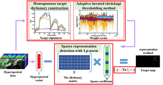
Graphical Abstract

1. Introduction

Hyperspectral images consist of both spectral and spatial information. Spectral information of hyperspectral images is of great abundance. Due to the advantage of rich spectral information, the spectral characteristics of hyperspectral imagery (HSI) can be used to differentiate similar substances from each other. With the development of sensor technology, hyperspectral target detection techniques have been used in a wide range of aspects of mineral exploration, agriculture, environmental monitoring, and information reporting [1,2]. Target detection is to search the desired targets, such as man-made targets, which popularly have different spectral signatures from natural background targets [3,4]. Hyperspectral target detection issue is equal to a binary hypothesis theory that contains two hypotheses: the H 1 (target is subsistent) and H 0 (target is absent) intrinsically.
Many traditional target detection algorithms have been proposed [5,6,7]. Constrained energy minimization (CEM) method is to design a filter that can output the smallest amount of information under the constraints of target spectrum. It can enhance target information and suppress the background information [8,9,10]. The CEM has better detection effect on the small objects in the image except for the large objects. There is no need to qualify that the data belongs to a particular distribution, spectral angle mapper (SAM) [11], which does not need any information distribution assumption, can be seen as one of the most simplest target detectors. Spectral matched filter (MF) [12,13] is also a well-known detector in maximizing signal-to-background ratio and estimating the background covariance matrix to acquire targets of necessary from background. Regularized spectral matched filter, which is the extension of SMF, has been recently investigated in Reference [14]. The generalized likelihood ratio test (GLRT) is considered when the covariance of background pixel is the same but the mean value is different [15]. With the progress of machine learning and pattern recognition, many information-driven target detection algorithms, such as kernel method and sparse expression method, have gradually attracted researchers’ attention on hyperspectral target detection. Kernel-based detectors include kernel RX, support vector data description (SVDD), and one-class support vector machine (OC-SVM) [16]. In addition, some linear combinations-based detectors have been developed to find objects in a minimum-residual manner [17,18].
In Reference [19,20], sparse representation detector (SRD) was proposed for target detection. For example, sparse representation with a binary hypothesis testing model was developed in Reference [21,22]. The approximate results can be calculated by samples from individual background dictionary or target and background mixed basis under different hypothesis [23]. Two approaches, called GPN and MPN, are designed to automatically detect targets from the hyperspectral remote sensing data [24]. Both methods are improved versions of NMF. The GPN uses an iterative projected gradient descent methods, while the iterative multiplicative gradient-based method is used in the MPN. Sparse and Low-Rank Matrix Decomposition (SLMD) is proposed to effectively detect targets in hyperspectral imagery with homogeneous representation [25]. The paper consists of two core modules. The first one involved with building an accurate background dictionary to help reduce the heterogeneous interference, and the second one is to build a target dictionary to further detect targets. A strategy of combining sparse and collaborative representations (CSCR) is introduced in Reference [26,27]. For each testing pixel, priori target signatures’s sparse representation is implemented by using the l 1 -norm minimization, while background pixel’s collaborative representation is implemented by using the l 2 -norm minimization. All target detection results are calculated by using the consequence from above two representation residuals. These methods fully exploited the fact the pixel from HSI can be approximated by a sparse linear representation based on specific observation basis. Sparsest representation coefficients can be obtained by solving an l 0 -norm optimization, which is NP-hard [28]. Alternatively, the  l 1 -minimization [29] has been employed in SRD, providing excellent performance.
Nevertheless, one of the drawbacks in the l 1 -minimization is that solutions are often less sparse than those in the l 0 -minimization. In SRD, the sparser the coding coefficients are, the easier the decision is. Based on this consideration, we attempt to develop a novel sparse representation detector with an alternative l p minimization which has a sparser solution than the l 1 -minimization. Hence, a non-convex l p -norm-based sparse representation detector (Lp-SRD) is proposed, which can recover a testing pixel by solving an l p -norm minimization issue with requirements of much feeble incoherence conditions and lower signal to background ratio for a stable solution [30].
The l p -norm sparse coding problem has been applied to a lot of fields of machine learning and computer vision tasks. Some people have studied the construction of dictionaries. The traditional complete dictionary contains target and background, which has certain influence on the performance of target detection. Moreover, some dictionaries are acquired by double-window method, which is low performance and less efficiency. Therefore, the method of constructing homogeneous target dictionary is proposed and used in Lp-SRD.
Some papers have made some efforts in solving the sparse coefficient. A few typical algorithms solving this problem include iteratively reweighted l 1 -minimization method (IRL1) [31], general iteratively reweight least squares method (GIRLS), iterative reweight least squares method (IRLS) [32], Look-Up Table method (LUT) [33], iteratively thresholding method (ITM) [34], and the generalized iterated shrinkage algorithm (GISA) [35]. Among these methods, IRLS, IRL1, and ITM usually cannot converge to global optimal solution, even for l p -minimization problem. LUT can employ look-up tables to reserve the solutions, e.g., different values for the same variable and regularization parameter, which requires high memory and computational costs to construct and reserve the look-up table. The convergence rate is slow to GISA. Thus, adaptive iterated shrinkage thresholding method (AISTM) is proposed and used to Lp-SRD.
The contributions of our research include: first, l p -minimization-based sparse representation is proposed for hyperspectral target detection; second, homogeneous target dictionary and adaptive iterated shrinkage thresholding method (AISTM) are proposed to solve the l p -minimization problem. Due to this overall design and optimization, higher purity reconstruction endmember will be obtained, thus resulting in smaller residuals for the correctly detected items of our method. The membership of y ( y R L are testing pixels, and L is the number of bands in the hyperspectral.) can be calculated by contrasting the final residual with the prescribed threshold η . Experimental results indicate that our Lp-SRD method is supreme to other counterparts with p ( 0 < p < 1 ).
The remaining part of our paper is arranged as follows. Existing sparse representation detector with L 1 -norm is introduced in Section 2. The Lp-SRD target detection architecture is given in Section 3. The hyperspectral datasets, parameters analysis and detection performance of correlative methods are displayed in Section 4. Last, the conclusion is summarized in Section 5.

2. Sparse Representation Detector with L 1 -norm

The basic idea of sparse representation is that all or most of the original signals can be sparsely reconstructed by the linear combination of elements from the dictionary. In Reference [36,37], SRD was designed to detect one (target) classes and reject other background classes. In our work, training data consist of target signatures. Background samples are not assumed to be known a priori. This is useful in practical applications to detect targets from unknown background.
Consider hyperspectral data with known target signatures X R L × N . The N denotes the number of atoms, and each atom has L dimensional features. The  y R L being a testing pixel. Then, y can be approximately represented as,
y α 1 x 1 + α 2 x 2 + + α N x N = x 1 x 2 x N α 1 α 2 α N T = X α ,
where α is weight vector and asked to be as sparse as possible. With a sparser α , it is easier to properly determine which category member the pixel y belongs to. Sparse vector α can be calculated by deducing the following equation,
α = arg min α 0 s . t . y = X α .
The solving of Equation (2) is NP-hard problem and its computational is quite large for solving large-scale problems [38]. Many researchers find it is strenuous to use above method to solve large-scale calculations. The  l 1 -norm can replace l 0 -norm [39] in Equation (2) under certain conditions. Moreover, y = X α cannot hold precisely since the testing pixel may include noise. Equation  (2) would be described as:
α = arg min α 1 + λ y X α 2 2 ,
where λ is Lagrange multiplier ( λ > 0 ), can have a balance between sparsity and data reconstruction error. For this optimization process, a few techniques can be used to estimate the solution [40]. When the sparse vector α is acquired, the residual of the pixel is described as:
r S R D ( y ) = y X α 2 .
In SRD, once the representation process is finished, target can be determined based on the residuals. And the residuals can be obtained by directly subtracting the reconstruction element from the original input. If  r S R D ( y ) is smaller than the predetermined threshold, y would be identified as target pixel; otherwise, y would be decided as background pixel.

3. Proposed Target Detection Framework

The sparse representation was originally designed for high-dimensional image data analysis. The idea is that the detected pixels can be expressed linearly by a very few atoms in the over-complete dictionary. The target detection algorithm by sparse representation in this paper mainly includes three aspects: (1) homogeneous target dictionary construction; (2) sparse coefficient solution; and (3) decision function design. The general flowchart for target detection method is shown in Figure 1. First, the dictionary matrix is constructed by calculating the mean of target spectrum and its four-neighborhood spectrum. Then, l p -norm is used to acquire the sparse coefficient, in which AISTM is used to acquire the sparse coefficient iteratively. Finally, an appropriate decision function is designed to judge the results.

3.1. Homogeneous Target Dictionary Construction

Target detection has been studied by many researchers in the area of HSI processing. At present, sparse representation algorithm has achieved good detection effect in this aspect. However, dictionaries in traditional sparse representation algorithms contain both target and background pixels, and the proportion of target information and background information is uncertain [41,42]. Different proportions of target and background will produce different detection results. In addition, the spectral curve of some pixels may be incorrect due to measurement errors or other reasons, so the dictionary cannot be accurately constructed. To overcome these shortcomings, the homogeneous target dictionary construction scheme is proposed. In our work, training data consist of target signatures. Each target spectral feature is obtained by the mean of its spectrum and its four-neighborhood spectrum. This is useful in practical applications to detect targets from an unknown background.
Consider hyperspectral data with known target signatures X R L × N , where L denotes the number of dimensional features for each atom. The N denotes the number of obtained target atoms. Dictionary X can be denoted as:
X = { x 1 , x 2 , , x i , , x N } ,
where x i is a priori target spectrum.
The position coordinates of x i is denoted as (i, j). Then, mean x i can be expressed as
x i = x i ( i , j ) + x i ( i 1 , j ) + x i ( i + 1 , j ) + x i ( i , j 1 ) + x i ( i , j + 1 ) 5 .

3.2. Sparse Representation Detector with L p -norm

The l p -norm is a function that has the concept of “length” [5]. It is denoted as
α p = i = 1 N α i p 1 / p .
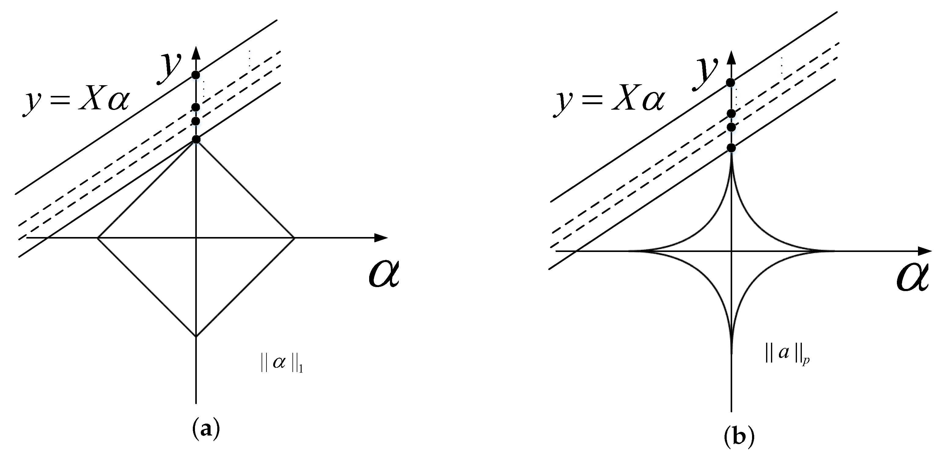
In order to clearly show the process for methods of different norm, we use the graphics in 2-D space to display the solutions for the l 1 -norm minimization in Figure 2a and l p -norm minimization in Figure 2b. S = α * : y = X α } expresses a line in the 2-D space, but, in the higher dimensions, it will be a hyperplane. The line of S covers all possible solution α * . Therefore, the sparse solutions for these methods are the intersection points of line S and the graphs of l 1 and l p . We can estimate whether the solutions are sparse by calculating the number of intersection points. Assume that we change the l p -ball from original condition until it touches the collection of S for some point. So, the solutions for the l p -norm minimization issue are above mentioned intersection points. When the sparse solutions are localized on the coordinate axis, they will be sparse enough. For the scenograph of Figure 2, we can clearly find out that the solutions for l p -norm minimization are sparser than l 1 -norm.
As we mentioned earlier, the matrix X is required to be less coherent [39] to ensure the equivalence between l 0 -minimization in Equation (2) and l 1 -minimization in Equation (3). Otherwise, the solution (weight vector) in the l 1 -minimization is less sparse than the one in the l 0 minimization [35]. Fortunately, the  l p -minimization has been proven that it can recover a sparser signal from linear measurements than the l 1 -minimization [43], which can be confirmed by both theoretical analysis and numerical simulations [44]. The objective function of the l p optimization in our paper can be denoted as
min α 1 2 y X α q q + λ α p p .
Better results can be achieved by setting the value of q ( 0 < q < 2 ) as an open solution to the reconstruction. This is a non-convex minimization issue as 0 < p < 1 , and  · p p is not sub-additive and violates the triangle inequality. Inspired by soft-thresholding, we propose adaptive iterated shrinkage thresholding method (AISTM) to obtain the l p -minimization solution in Equation (8) by two steps: (1) modifying the thresholding and (2) modifying the shrinkage means.
When y > 0 , solutions for Equation (8) would satisfy the range of [ 0 , y ] . Otherwise, solutions for Equation (8) will fall into the range of [ y , 0 ] . Specifically, we focus on the situation of y > 0 in the following. We can construct a function g ( α ) as
g ( α ) = 1 2 ( α y ) 2 + λ | α | p .
First, it is found that, when we obtain λ and p, there is a specific threshold τ p A I S T M ( λ ) . If  y < τ p A I S T M ( λ ) , α = 0 would be the global minimum. Otherwise, the nonzero solution would be the optimal. Considering for any y τ p A I S T M ( λ ) , + , g ( α ) has one unique minimum α p * in the scope of ( α 0 ( λ , p ) , + ) . We can get the following equation as
α p * y + λ p α p * p 1 = 0 .
For any y τ p A I S T M ( λ ) , + , we let α p * become the unique minimum for g ( α ) in the scope of ( α p * , + ) . Accordingly, we can get the following equation as
g ( 0 ) > g ( α p * ) .
Further, to generalize soft threshold, we would solve the following equation set to acquire the appropriate thresholding τ p A I S T M ( λ ) and α p * corresponding with thresholding as
α p * τ p A I S T M ( λ ) + λ p α p * p 1 = 0 1 2 α p * τ p A I S T M ( λ ) 2 + λ α p * p = 1 2 τ p A I S T M ( λ ) 2 ,
where the only solution for α p * is
α p * = ( 2 λ ( 1 p ) ) 1 2 p ,
and the thresholding value τ p A I S T M ( λ ) is
τ p A I S T M ( λ ) = ( 2 λ ( 1 p ) ) 1 2 p + λ p ( 2 λ ( 1 p ) ) p 1 2 p .
Secondly, in order to shorten the time of finding the non-zero solution, the following gradient descent method is adopted:
α k = α k 1 λ m ^ k / ( s ^ k + ε ) ,
where λ is the stepsize, and  ε is equal to 1 × 10⁻⁸ to prevent zeros from occurring in the implementation. And  m ^ k and s ^ k can be obtained as
g k = λ p α k 1 p 1 m k = β 1 m k 1 + 1 β 1 g k s k = β 2 s k 1 + 1 β 2 g k 2 m ^ k = m k / 1 β 1 k s ^ k = s k / 1 β 2 k ,
where g k is gradient. The  λ is learning rate. The  m k is biased first moment estimate, and  s k is biased second raw moment estimate. The  m ^ k and s ^ k are bias-corrected. The  β 1 is exponential decay rate of first order moment estimation. The  β 2 is exponential decay rate of the second moment estimation. We assign the value of β 1 and β 2 to 0.1 and 0.2, respectively. The iterative algorithm AISTM ( y , λ , β 1 , β 2 , ε , J , u ) is summarized in Algorithm 1.
Algorithm 1 (AISTM):  T u A I S T M ( y ; λ ) = A I S T M ( y , λ , β 1 , β 2 , ε , J , u )
Input: y , λ , β 1 , β 2 , ε , J , u
1. Calculating the thresholding value τ u A I S T M by Equation (14);
2. If  y τ u A I S T M ( λ ) ;
3.    T u A I S T M ( y ; λ ) = 0 ;
4. Else
5.   k = 0 , α ( k ) = y ;
6.   k = 0 , m k = 0 , s k = 0 ;
7.  Iterate on k = 0 , 1 , 2 , , J ;
8.  Calculating the corresponding α u * by Equation (15);
9.   T u A I S T M ( y ; λ ) = sgn ( y ) α u * ;
10. End
Output: T u A I S T M ( y ; λ ) .
AISTM is an improvement for iterative shrinkage thresholding. It has been proven the ITM algrithm would converge to stationary point in Reference [45], while any thresholding T ( y ; λ ) satisfied with 0 λ < + and < y < + , if T ( y ; λ ) has the following characteristics:
(i)
T ( y ; λ ) T y ; λ if y y ;
(ii)
T ( y ; λ ) = T ( y ; λ ) ;
(iii)
lim y T ( y ; λ ) = ; and
(iv)
0 T ( y ; λ ) y for 0 y < .
We can easily find that AISTM satisfies above four characteristics. So, the ability of convergence for AISTM method would be guaranteed.
In the proposed method, alternating direction method of multipliers (ADMM) is taken to settle SRD framework. We replace the soft-thresholding operator of ADMM by using AISTM operator method. By choosing the appropriate value of u (q or p) for AISTM, we can get good detection results. The AISTM is an iterative algorithm, and the gradient descent method for X or y in iteration process is involved as
α ( k ) = T u A I S T M ( α ( k 1 ) X 2 X T ( X α y ) ; X 2 λ ) ,
where X is the spectral norm of X .
Empirically, we find that satisfactory results can be acquired by choosing the number of iterations J as 2 or 3. When α is obtained, membership of y can be determined by comparing final residual with prescribed threshold η :
D Lp - SRD ( y ) = 1 if y X α 2 < = η 0 if y X α 2 > η ,
where 1 means that y is a target, and 0 means that y belongs to the background [46].
To illustrate the advantages of the proposed Lp-SRD, Figure 3 depicts an example of different methods in reconstruction residuals between a target or background pixel and its estimation using the HyMap data to be introduced in Section 4. The target spectrum represents a pixel of yellow nylon, and the background spectrum represents a mixture of grass and building. From comparative results shown in Figure 3a, the reconstruction residual of the proposed Lp-SRD between a chosen target pixel and its estimation is relatively small, which indicates the reconstructed spectrum of Lp-SRD is closer to that of a real target pixel. The residual is closely correlated with detection results, and the smaller the reconstruction residual is, the more likely the pixel will be claimed as a target one. On the other hand, in Figure 3b, the reconstruction residual of the proposed Lp-SRD between a chosen background pixel and its estimate is relatively large; this makes it convenient to distinguish the target from its background. In this way, the solution for l p -norm minimization would become more stable, resulting in better detection ability.

4. Experiments and Discussion

4.1. Hyperspectral Datasets

The first dataset is the scene diagram of Gulfport area. The image was obtained by Airborne Infrared or Visible Image Spectrometer (AVIRIS) sensor [47]. The image is made up of 100 × 100 pixels, and the image’s spatial resolution is about 3.4 m. Gulfport contains 191 spectral bands after removing corresponding bands. The targets are the three airplanes. The false color and ground-truth map for targets are displayed in Figure 4.
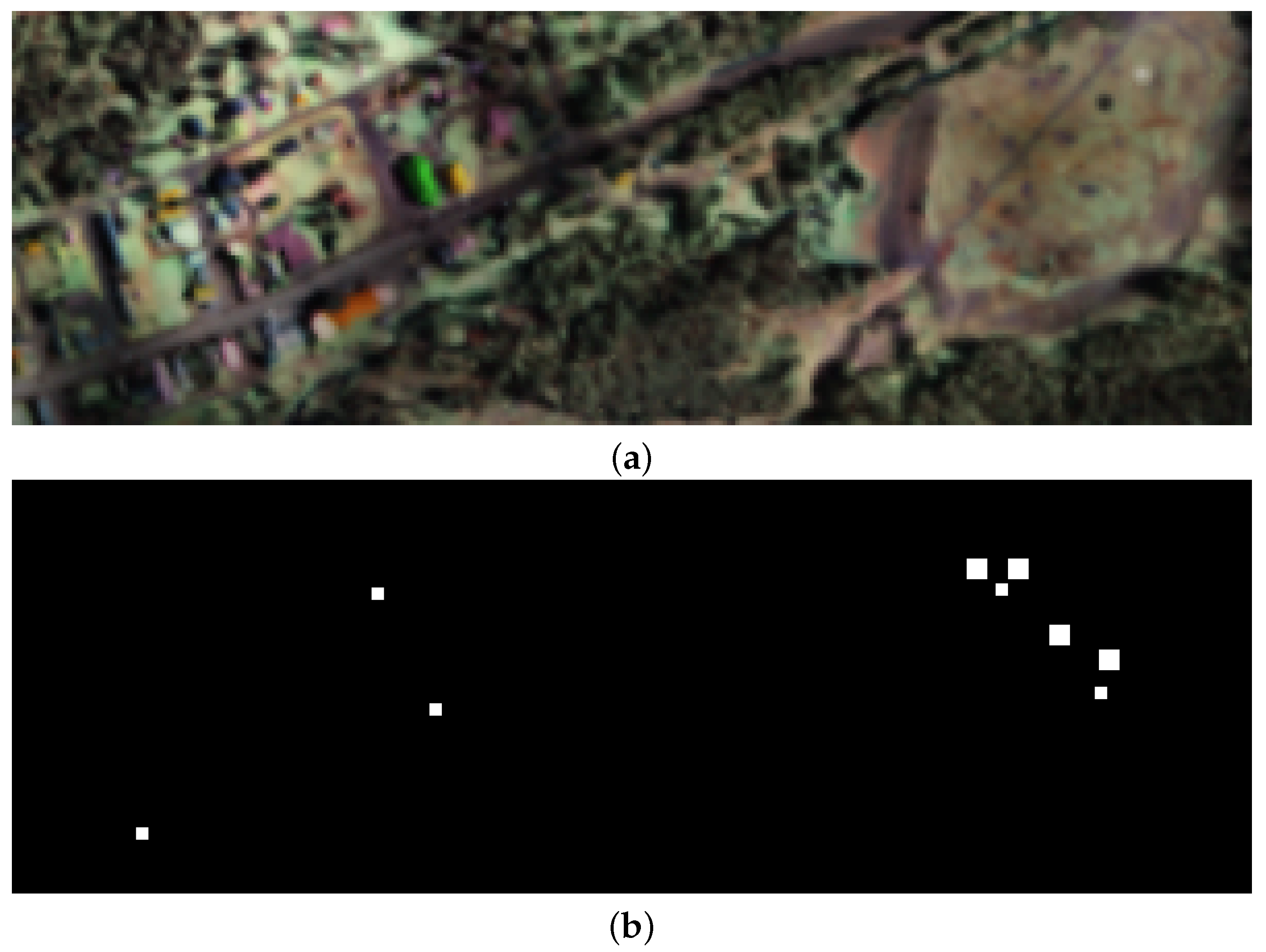
The second dataset is the scene diagram of Cooke City area, Montanta, on 4 July 2006. The image was obtained by HyMap hyperspectral imagery sensor [48]. The image is made up of 200 × 800 pixels, and the HyMap’s spatial resolution is about 3 m. HyMap contains 126 spectral bands meet wavelength interval 0.4–2.5 μ m. In order to compare quickly, we tailor a subgraph for the size 100 × 300 in the paper. Experimental results are satisfactory. Seven targets’ signatures are used for training, which includes 4 fabric panel targets (Yellow Nylon, Red Nylon, Red Cotton, and Blue Cotton) and 3 vehicle targets (Chevy Blazer, Subaru GL Wagon, and Toyota T100). Vehicle targets are located in the right half of the false color map. Panel targets are located in the left half of the false color map. The false color and ground-truth map for targets are displayed in Figure 5.
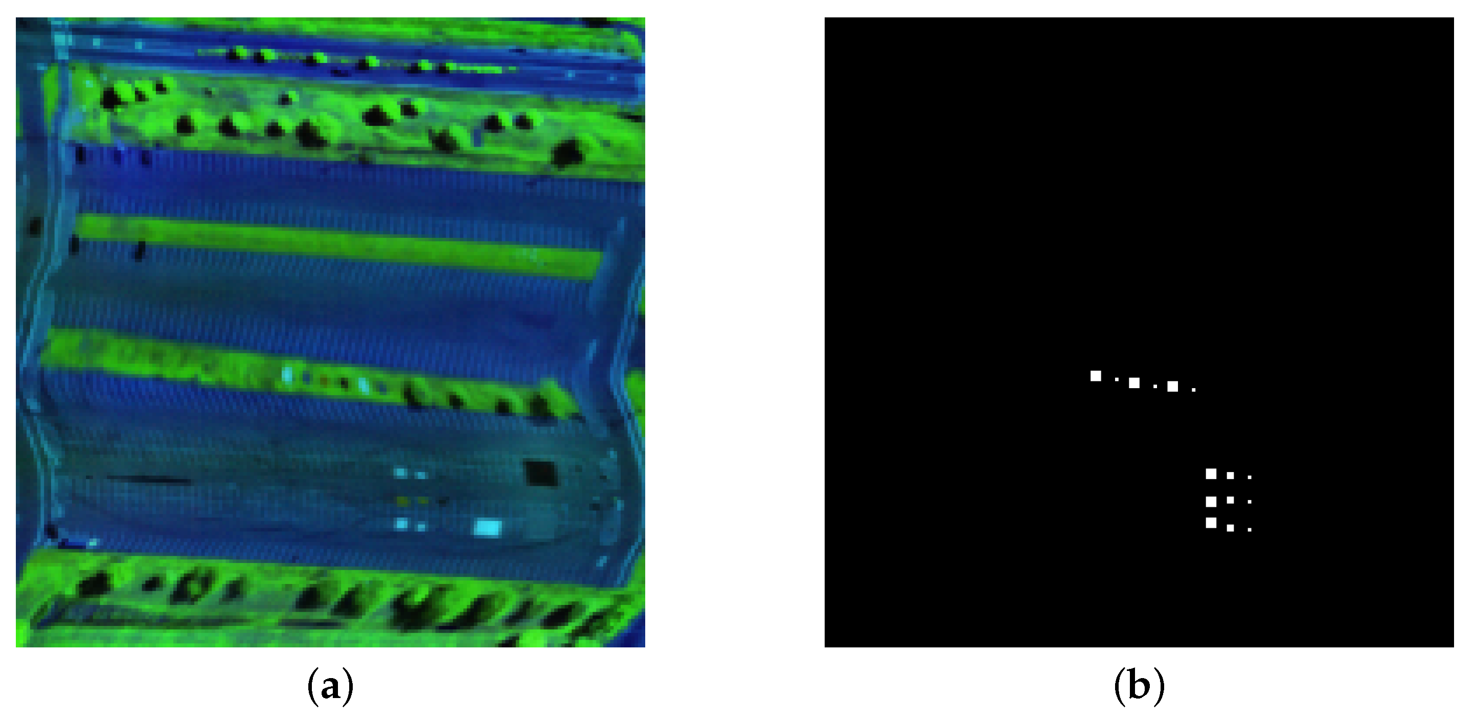
The third dataset is comes from Rochester experiment. The image was obtained by SpecTIR hyperspectral sensor. The image is made up of 180 × 180 × 120 pixels, and SpecTIR’s spatial resolution is about 1 m. The noisy and useless bands have been deleted in this image. Targets contain man-made colorful square fabrics [49]. The false color and ground-truth map for targets are displayed in Figure 6.
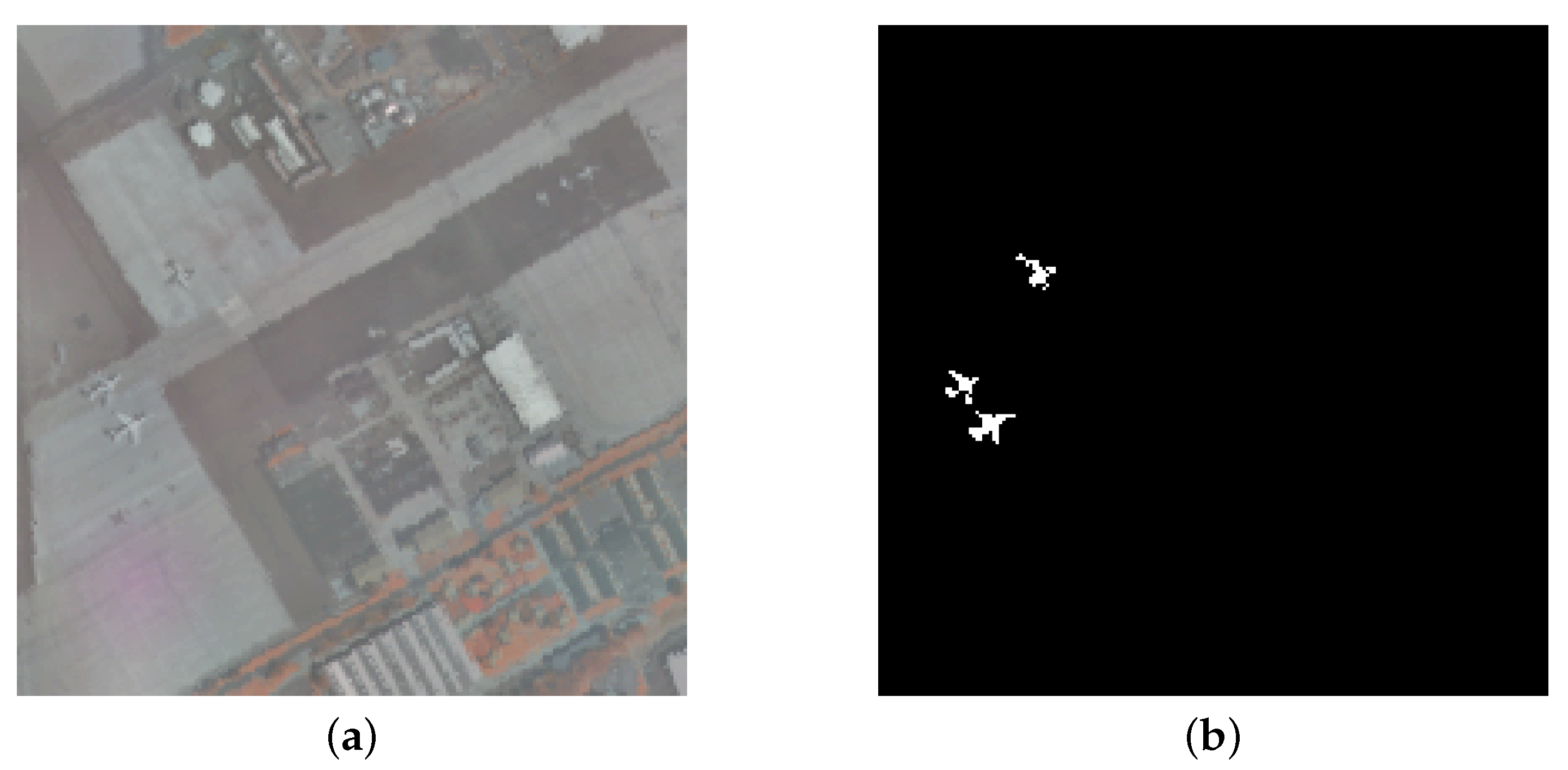
The fourth dataset is the scene diagram of San Diego. The image was obtained by AVIRIS sensor. The image is made up of 200 × 200 × 189 pixels, and San Diego’s spatial resolution is about 3.5 m. The noisy and useless bands have been deleted in this image. Targets consist of airplanes containing fifty-eight pixels [50]. The false color and ground-truth map for targets are displayed in Figure 7.

4.2. Parameters Analysis

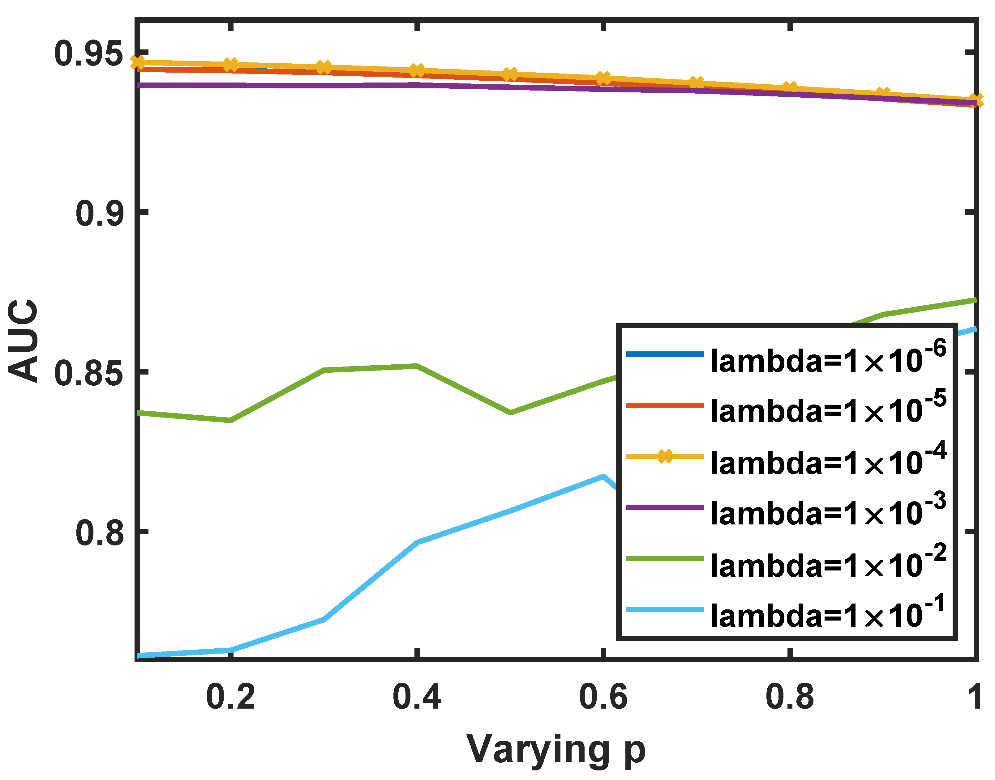
For the proposed Lp-SRD, the value of dictionary samples for the Gulfport dataset, the HyMap dataset, the SpecTIR dataset and the San Diego dataset are 3, 7, 5, and 3. The values of u (q) are 0.9, 1.2, 1.2, and 1, respectively. Two parameters (p and λ ) are studied. These two parameters are very important for the proposed algorithm, and only by choosing the right parameters can the best detection performance be obtained. By fixing λ as {1 × 10⁻⁶, 1 × 10⁻⁵, 1 × 10⁻⁴, 1 × 10⁻³, 1 × 10⁻², 1 × 10⁻¹} as suggested in Reference [35], and varying p from 0.1 to 1.0 at intervals of 0.1, the detection performance of Lp-SRD under different parameters are collected. Figure 8, Figure 9, Figure 10 and Figure 11 can be used to analysis the detection performance with different parameters.
Figure 8, Figure 9, Figure 10 and Figure 11 show the area under curve (AUC) performance of our proposed Lp-SRD by varying p, as well as λ . According to Equation (9), p can affect the performance of the detector. Here, p is changed from 0.1 to 1.0. In the Gulfport dataset, one can observe the detection performance in Figure 8 when the parameter λ = 1 × 10 2 and the parameter p is varied. For example, when p = 0.9, the proposed Lp-SRD achieves the highest detection accuracy, i.e., AUC = 99.65%, and drops around 97.58% as p = 0.1. In the HyMap dataset, one can observe the detection performance in Figure 9 when the parameter λ = 1 × 10 4 and the parameter p is varied. For example, when p = 0.1, the proposed Lp-SRD achieves the highest detection accuracy, i.e., AUC = 94.48%, and drops around 93.84% as p = 1.0. In the SpecTIR dataset, one can observe the detection performance in Figure 10 when the parameter λ = 1 × 10 1 and the parameter p is varied. For example, when p = 0.1, the proposed Lp-SRD achieves the highest detection accuracy, i.e., AUC = 99.70%, and drops around 96.50% as p = 0.5. In the San Diego dataset, one can observe the detection performance in Figure 11 when the parameter λ = 1 × 10 1 and the parameter p is varied. For example, when p = 0.4, the proposed Lp-SRD achieves the highest detection accuracy, i.e., AUC = 98.99%, and drops around 98.84% as p = 1. These figures also show the detection performance versus varying λ . A wide range of λ is from {1 × 10⁻⁶, 1 × 10⁻⁵, …, 1 × 10⁻¹}. We notice that the detection performance is relatively excellent if the parameter p and λ are fixed. Therefore, p and λ can be set to corresponding values to improve the detection performance of this method.

4.3. Detection Performance

We contrast the detection performance between Lp-SRD method and other detection methods, such as CEM, OC-SVM, SRD, etc. For qualitative and quantitative comparison, detection maps, statistical separability analysis, receiver operate characteristic (ROC), and area under the curve (AUC) metric are introduced for main criteria for evaluation. ROC curves have been far and wide employed as the performance estimate means for target detection situations, where it indicates the comparison between target detection probability p d and false alarm rate p f . The computational equation of p d and p f can be denoted as
p d = N detected N t p f = N miss N ,
where N detected denotes the number of detected right target pixels under threshold η , N miss denotes the number of background are mistaken for targets, N t denotes the number of practical target pixels in HSI, and N is the number of all pixels in HSI.
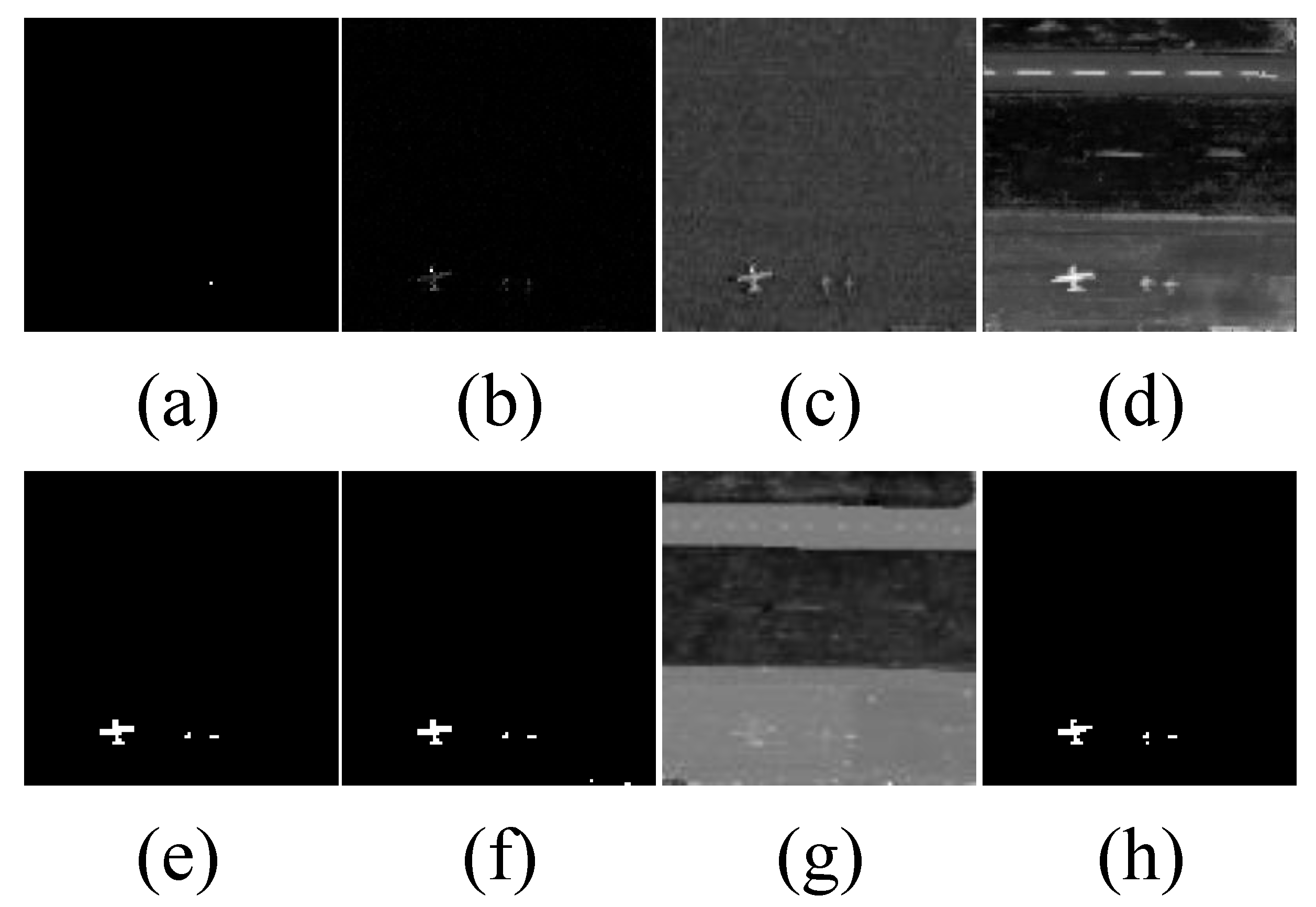
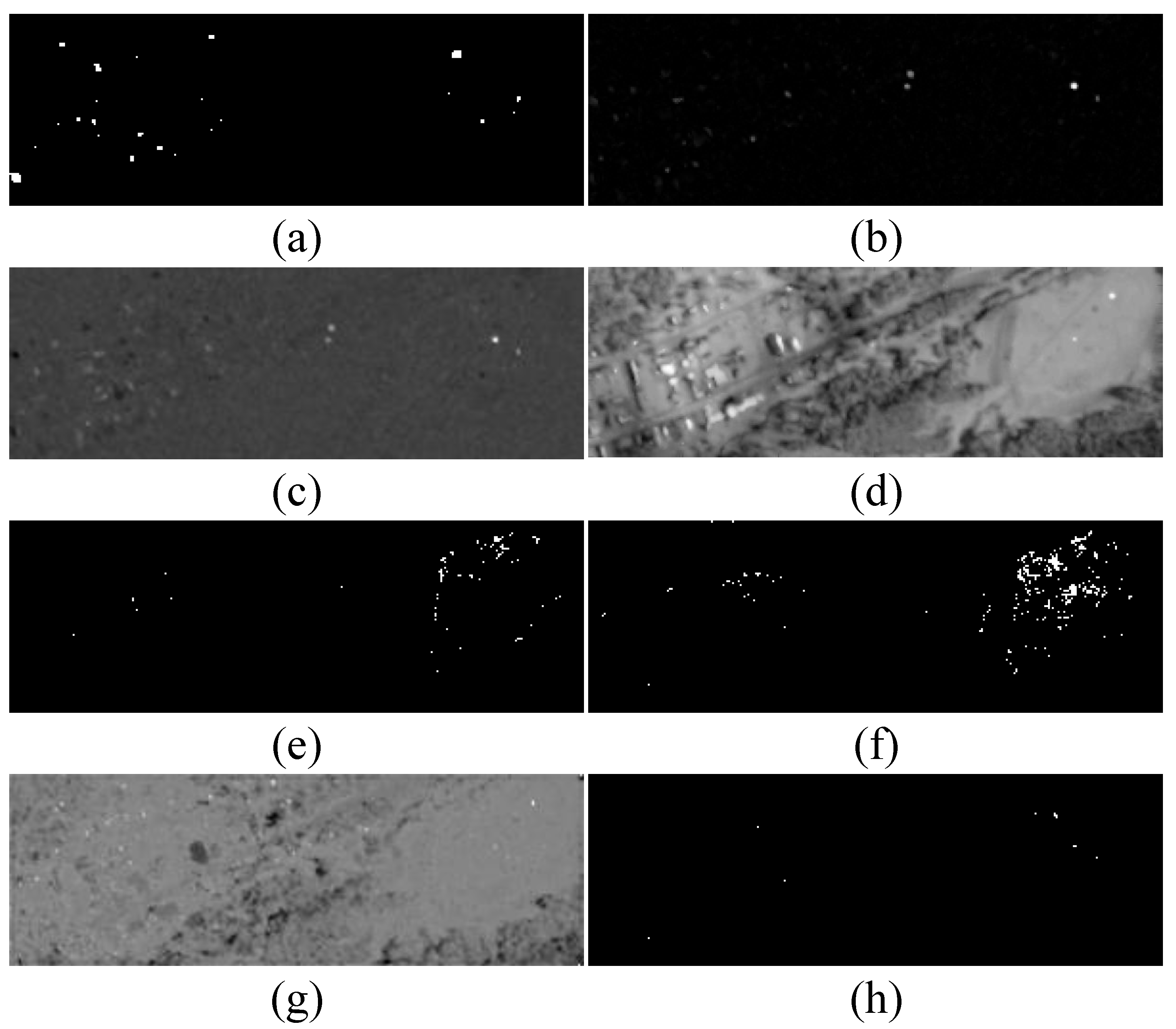
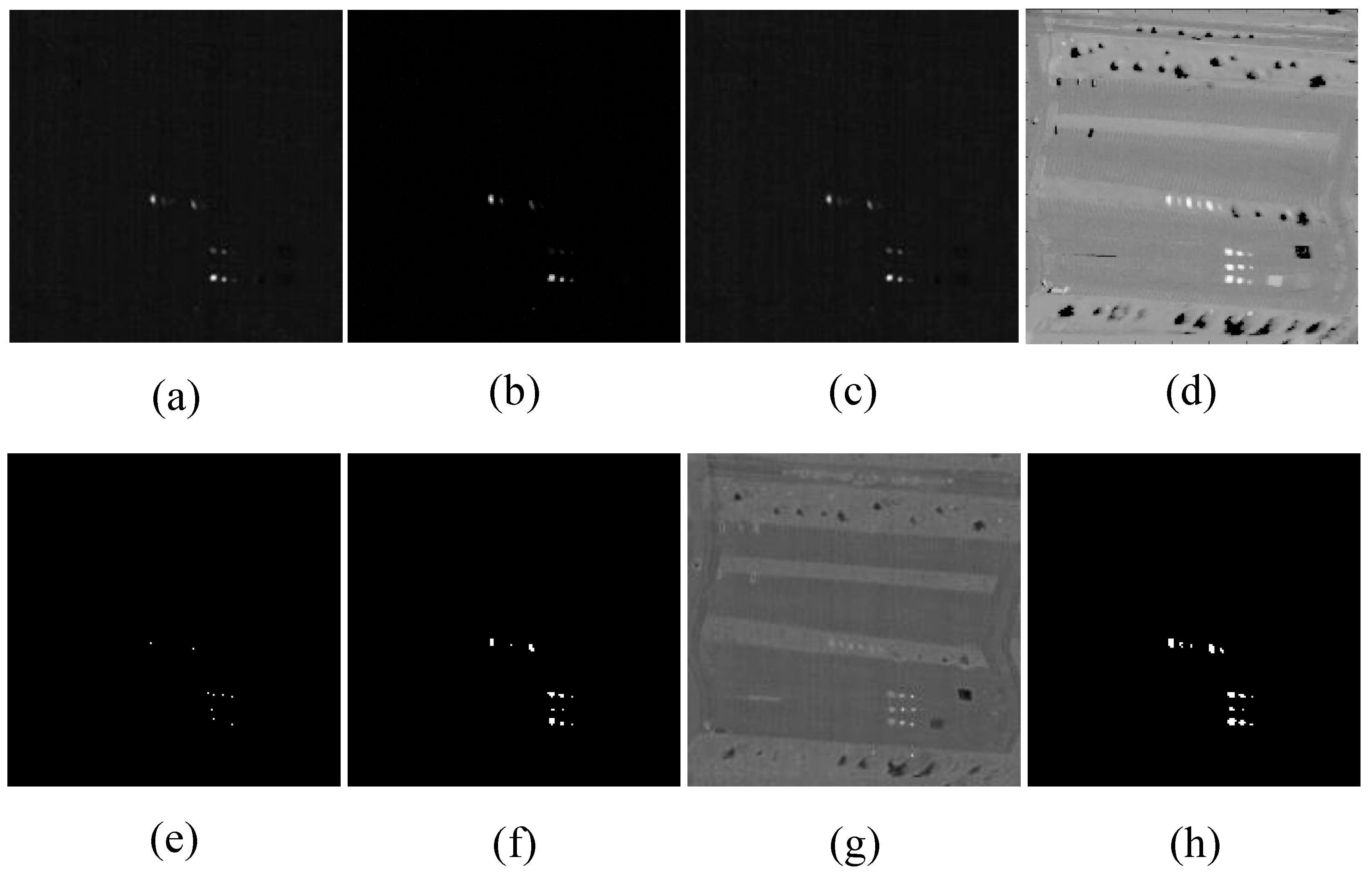
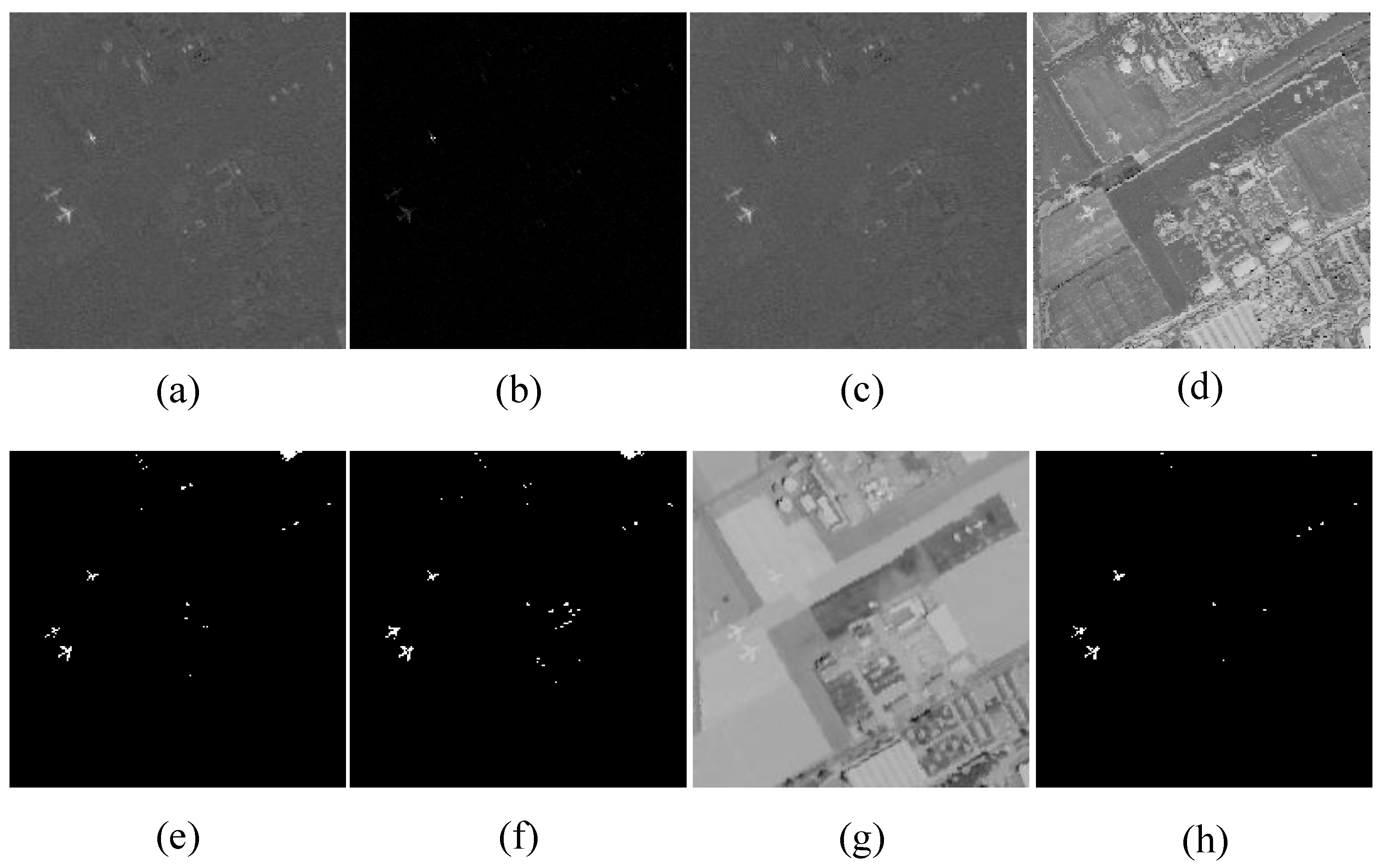
Figure 12, Figure 13, Figure 14 and Figure 15 denote the detection maps under p f is fixed to a appropriate value (e.g., 0.1 or 0.15) and p d is the corresponding value. The p d for proposed Lp-SRD from Figure 12, Figure 13, Figure 14 and Figure 15 are 1.00, 0.94, 1.00, and 1.00, respectively. The proposed Lp-SRD reflects the best detection results with the largest p d . When p f is set to a appropriate value, a suitable threshold η can be acquired.
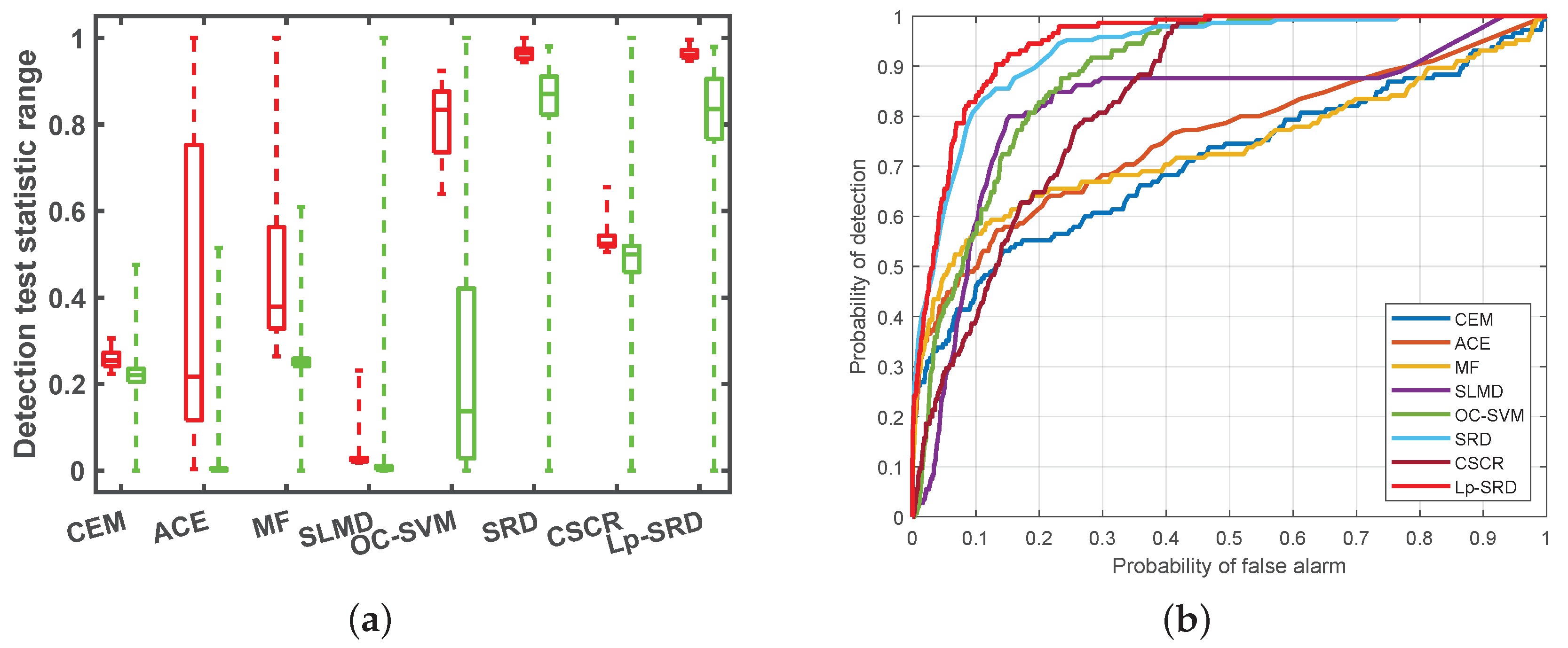
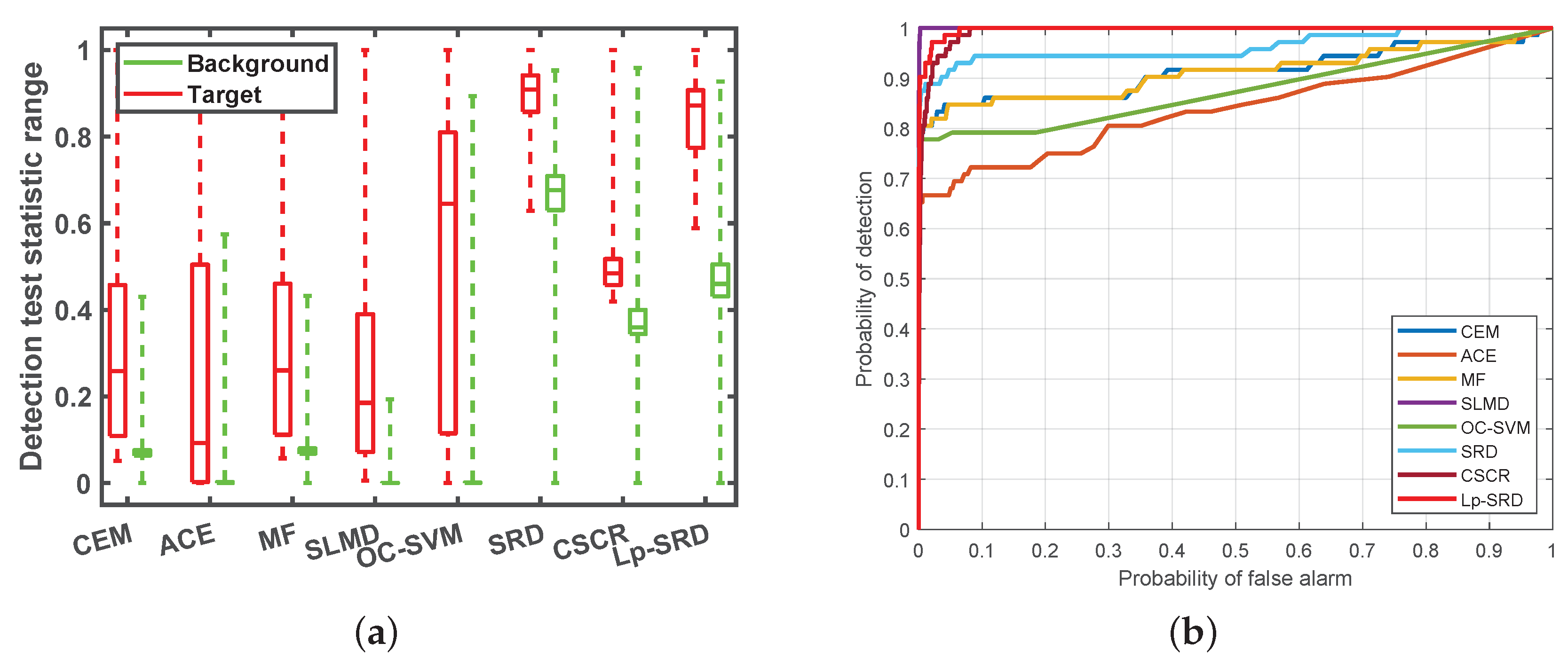
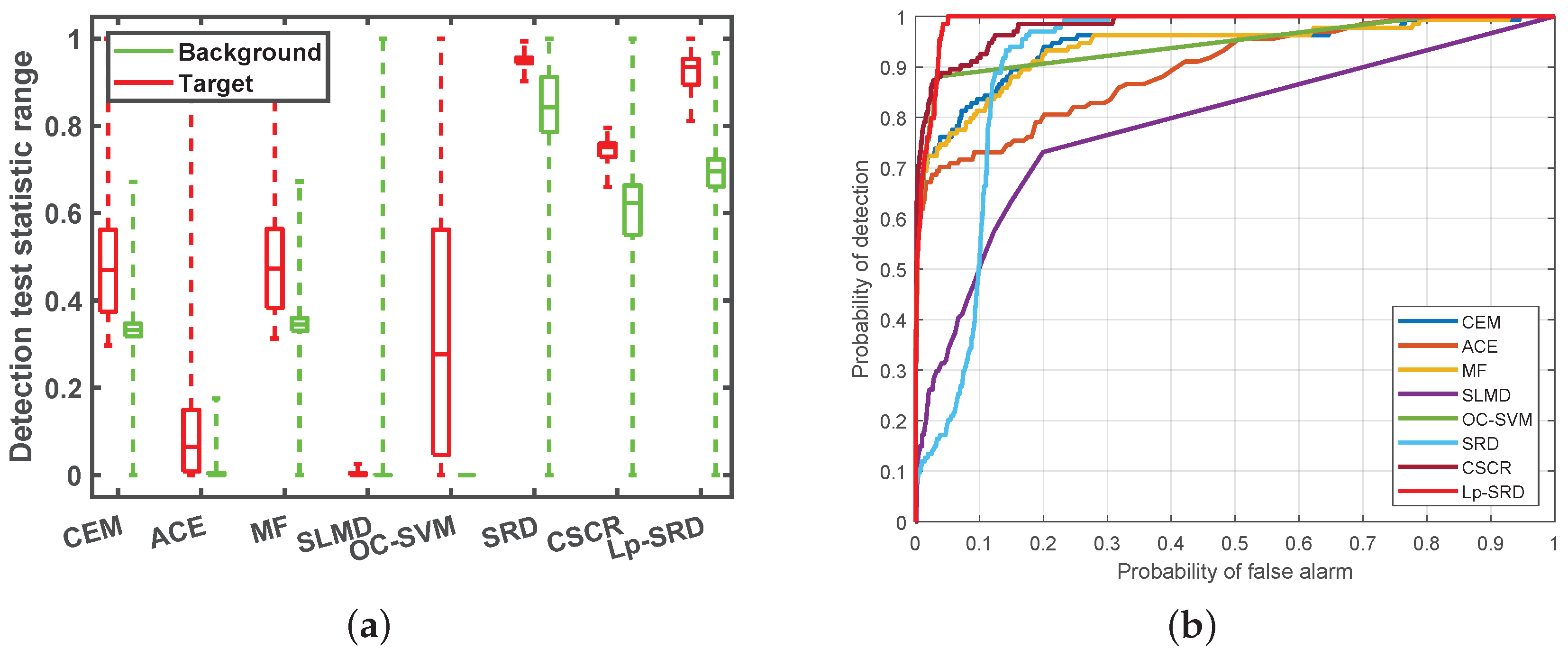
Figure 16, Figure 17, Figure 18 and Figure 19 illustrate the statistical separability analysis and ROC of the aforementioned detectors. Figure 16a, Figure 17a, Figure 18a, Figure 19a stand for box diagrama, and Figure 16b, Figure 17b, Figure 18b, Figure 19b stand for ROC for 4 real hypserspectral datasets. Next, we discuss the detection performance for the proposed method through box diagram and ROC curve, respectively.
First, the box diagrama is analyzed. The red box represents a range of targets, and the green box represents range of background. The interval between the green and red boxes shows separability between target and background. As shown in Figure 16a, the interval between the red and green boxes of Lp-SRD method is larger than other mentioned methods. It shows that Lp-SRD can easily separate targets from the background more useful. As shown in Figure 16a, Figure 17a, Figure 18a, Figure 19a, the box diagrams of the other three data also show that our proposed method can also easily separate the target from background.
Second, we analyzed the ROC. For generating ROC, detection output results are normalized to [ 0 , 1 ] as the value of threshold are gradually altered for 0 to 1. By calculating the owned ground-truth map, ROC curve is acquired by drawing results probability of detection against the probability of false alarms at various threshold settings. The proposed Lp-SRD is validated with four real hyperspectral scenarios. Specifically, Lp-SRD yields a higher probability of detection with false alarm rate varies under a big range for Gulfport data, as shown in Figure 16b. For example, when p f is about ( 0.1 ), p d of Lp-SRD achieves approximately 1.0. The CEM, ACE, MF, SLMD, OC-SVM, SRD, and CSCR are are below 0.98. We can find the proposed Lp-SRD also provides the best performance for the other three data from Figure 16b, Figure 17b, Figure 18b, Figure 19b.
Table 1 further lists the AUC values for eight aforementioned detectors. For the four hyperspectral datasets, the AUC values for the proposed method are 0.9960, 0.9468, 0.9970, and 0.9899, respectively. The maximum AUC values of other methods for the four hyperspectral datasets are 0.9908, 0.9303, 0.9932, and 0.9805, which are all lower than that of the proposed method. Table 2 provides the execution time for various detection methods. For the four hyperspectral datasets, the execution time of the proposed method are 0.8816, 4.8677, 2.1889, and 3.6604, respectively. The execution time of the baseline method basically does not exceed 1 s. The detection time of the proposed method is between 1 and 5 s, which takes longer time than other baseline methods. It is apparent that we proposed Lp-SRD can realize the outstanding performance, although execution time is relatively larger than other traditional detection methods, except SLMD and CSCR. All experiments were implemented in MATLAB on an Intel Core i7-8700H CPU computer with 8 GB of RAM. Because OC-SVM code is used, we used MEX function that called C program for MATLAB. The proposed method has not yet been integrated into the toolkit and will be accelerated in the future. There is great potential for improvement in the computing efficiency.
From qualitative and quantitative analysis of the detection results, the proposed Lp-SRD is always superior to the CEM, ACE, MF, SLMD, OC-SVM, SRD, and CSCR. It can be confirmed that the non-convex l p -norm sparse coding solved by homogeneous target dictionary construction and adaptive iterated shrinkage thresholding method requires much weaker incoherence constraint conditions to acquire a good recovery.

5. Conclusions

For this paper, we presented an HSI target detection method named Lp-SRD. The method effectively investigated the minimum coefficient and made it possible to reach high detection accuracy with only limited hyperspectral priori information. Specifically, we designed a dictionary construction method based on homogeneous target dictionary. There were no background samples, libraries, nor local window involved in the operation procedure. Then, we proposed adaptive iterated shrinkage thresholding method to solve the l p -minimization problem. The algorithm contains two parts: modifying the thresholding and modifying the shrinkage rules. Last, target detection was achieved according to representation residual. Four real hyperspectral datasets were used to check detection performance for our proposed Lp-SRD method. Experimental results demonstrated the detection performance of the proposed method is improved by about 10 % to 30 % than methods mentioned in the paper.

Author Contributions

All the authors designed and participated in the research. X.Z. implemented the experiments. W.L. and M.Z. analyzed the overall construction of the draft. X.Z., W.L. and M.Z. completed the first draft. R.T., W.L. and P.M. reviewed the manuscript. All authors have read and agreed to the published version of the manuscript.

Funding

This work was supported by National Natural Science Foundation of China (NSFC-61922013, U1833203, 61421001), China Postdoctoral Science Fundation (2020M670163).

Acknowledgments

All the authors feel grateful the publicists of Gulfport hyperspectral dataset, HyMap hyperspectral dataset, SpecTIR hyperspectral dataset, and San Diego hyperspectral dataset. In this paper, these dataset are adopted to check the performance of our proposed Lp-SRD method. The authors also thank the all authors of the baseline methods for contrast experiments.

Conflicts of Interest

All the authors state that there is no conflict of interest.

References

  1. Schweizer, S.M.; Moura, J.M.F. Hyperspectral imagery: Clutter adaptation in anomaly detection. IEEE Trans. Inf. Theory 2000, 46, 1855–1871. [Google Scholar] [CrossRef]
  2. Datt, B.; McVicar, T.R.; Van Niel, T.G.; Jupp, D.L.; Pearlman, J.S. Preprocessing EO-1 Hyperion hyperspectral data to support the application of agricultural indexes. IEEE Trans. Geosci. Remote Sens. 2003, 41, 1246–1259. [Google Scholar] [CrossRef] [Green Version]
  3. Zhang, G.; Zhao, S.; Li, W.; Du, Q.; Ran, Q.; Tao, R. HTD-Net: A Deep Convolutional Neural Network for Target Detection in Hyperspectral Imagery. Remote Sens. 2020, 12, 1489. [Google Scholar] [CrossRef]
  4. Fu, X.; Shang, X.; Sun, X.; Yu, H.; Song, M.; Chang, C.-I. Underwater Hyperspectral Target Detection with Band Selection. Remote Sens. 2020, 12, 1056. [Google Scholar] [CrossRef] [Green Version]
  5. Zhang, Z.; Xu, Y.; Yang, J.; Li, X.; Zhang, D. A Survey of Sparse Representation: Algorithms and Applications. IEEE Access 2015, 490–530. [Google Scholar] [CrossRef]
  6. Zhang, L.; Zhang, L.; Tao, D.; Huang, X.; Du, B. Hyperspectral Remote Sensing Image Subpixel Target Detection Based on Supervised Metric Learning. IEEE Trans. Geosci. Remote Sens. 2014, 52, 4955–4965. [Google Scholar] [CrossRef]
  7. Zhang, Y.; Wu, K.; Du, B.; Zhang, L.; Hu, X. Hyperspectral Target Detection via Adaptive Joint Sparse Representation and Multi-Task Learning with Locality Information. Remote Sens. 2017, 9, 482. [Google Scholar] [CrossRef] [Green Version]
  8. Yang, S.; Shi, Z. SparseCEM and SparseACE for Hyperspectral Image Target Detection. IEEE Geosci. Remote Sens. Lett. 2014, 11, 2135–2139. [Google Scholar] [CrossRef]
  9. Wang, Y.; Lee, L.C.; Xue, B.; Wang, L.; Song, M.; Yu, C.; Li, S.; Chang, C.I. A Posteriori Hyperspectral Anomaly Detection for Unlabeled Classification. IEEE Trans. Geosci. Remote Sens. 2018, 56, 3091–3106. [Google Scholar] [CrossRef]
  10. Chang, C.I.; Li, H.C.; Song, M.; Liu, C.; Zhang, L. Real-Time Constrained Energy Minimization for Subpixel Detection. IEEE J. Sel. Top. Appl. Earth Obs. Remote Sens. 2015, 8, 2545–2559. [Google Scholar] [CrossRef]
  11. Li, W.; Du, Q. A survey on representation-based classification and detection in hyperspectral remote sensing imagery. Pattern Recognit. Lett. 2016, 83P2, 115–123. [Google Scholar] [CrossRef]
  12. Tao, R.; Zhao, X.D.; Li, W.; Li, H.C.; Du, Q. Hyperspectral anomaly detection by fractional fourier entropy. IEEE J. Sel. Top. Appl. Earth Obs. Remote Sens. 2019, 12, 4920–4929. [Google Scholar] [CrossRef]
  13. Funk, C.C.; Theiler, J.; Roberts, D.A.; Borel, C.C. Clustering to improve matched filter detection of weak gas plumes in hyperspectral thermal imagery. IEEE Trans. Geosci. Remote Sens. 2001, 39, 1410–1420. [Google Scholar] [CrossRef] [Green Version]
  14. Scharf, L.L.; Friedlander, B. Matched subspace detectors. IEEE Trans. Signal Process. 1994, 42, 2146–2157. [Google Scholar] [CrossRef] [Green Version]
  15. Theiler, J.; Foy, B.R. EC-GLRT: Detecting Weak Plumes in Non-Gaussian Hyperspectral Clutter Using an Elliptically-Contoured Generalized Likelihood Ratio Test. In Proceedings of the IGARSS 2008—2008 IEEE International Geoscience and Remote Sensing Symposium, Boston, MA, USA, 7–11 July 2008. [Google Scholar] [CrossRef] [Green Version]
  16. Li, W.; Du, Q. Collaborative representation for hyperspectral anomaly detection. IEEE Trans. Geosci. Remote Sens. 2014, 53, 1463–1474. [Google Scholar] [CrossRef]
  17. Lo, E. Partitioned correlation model for hyperspectral anomaly detection. Opt. Eng. 2015, 54, 123114. [Google Scholar] [CrossRef]
  18. Jablonski, J.A.; Bihl, T.J.; Bauer, K.W. Principal component reconstruction error for hyperspectral anomaly detection. IEEE Geosci. Remote Sens. Lett. 2015, 12, 1725–1729. [Google Scholar] [CrossRef]
  19. Chen, Y.; Nasrabadi, N.M.; Tran, T.D. Simultaneous joint sparsity model for target detection in hyperspectral imagery. IEEE Geosci. Remote Sens. Lett. 2011, 8, 676–680. [Google Scholar] [CrossRef]
  20. Chen, Y.; Nasrabadi, N.M.; Tran, T.D. Sparse representation for target detection in hyperspectral imagery. IEEE J. Sel. Top. Signal Process. 2011, 5, 629–640. [Google Scholar] [CrossRef]
  21. Zhang, Y.; Du, B.; Zhang, L. A sparse representation-based binary hypothesis model for target detection in hyperspectral images. IEEE Trans. Geosci. Remote Sens. 2014, 53, 1346–1354. [Google Scholar] [CrossRef]
  22. Du, B.; Zhang, Y.; Zhang, L.; Tao, D. Beyond the Sparsity-Based Target Detector: A Hybrid Sparsity and Statistics-Based Detector for Hyperspectral Images. IEEE Trans. Image Process. 2016, 25, 5345–5357. [Google Scholar] [CrossRef] [PubMed]
  23. Cui, M.; Prasad, S. Class-Dependent Sparse Representation Classifier for Robust Hyperspectral Image Classification. IEEE Trans. Geosci. Remote Sens. 2015, 53, 2683–2695. [Google Scholar] [CrossRef]
  24. Karoui, M.S.; Benhalouche, F.Z.; Deville, Y.; Djerriri, K.; Weber, C. Partial Linear NMF-Based Unmixing Methods for Detection and Area Estimation of Photovoltaic Panels in Urban Hyperspectral Remote Sensing Data. Remote Sens. 2019, 11, 2164. [Google Scholar] [CrossRef] [Green Version]
  25. Bitar, A.W.; Cheong, L.F.; Ovarlez, J.P. Sparse and Low-Rank Matrix Decomposition for Automatic Target Detection in Hyperspectral Imagery. IEEE Trans. Geosci. Remote Sens. 2019, 57, 5239–5251. [Google Scholar] [CrossRef] [Green Version]
  26. Li, W.; Du, Q.; Zhang, B. Combined sparse and collaborative representation for hyperspectral target detection. Pattern Recognit. 2015, 48, 3904–3916. [Google Scholar] [CrossRef]
  27. Tan, K.; Hou, Z.; Wu, F.; Du, Q.; Chen, Y. Anomaly Detection for Hyperspectral Imagery Based on the Regularized Subspace Method and Collaborative Representation. Remote Sens. 2019, 11, 1318. [Google Scholar] [CrossRef] [Green Version]
  28. Wright, J.; Yang, A.Y.; Ganesh, A.; Sastry, S.S.; Ma, Y. Robust face recognition via sparse representation. IEEE Trans. Pattern Anal. Mach. Intell. 2008, 31, 210–227. [Google Scholar] [CrossRef] [Green Version]
  29. Charles, A.S.; Olshausen, B.A.; Rozell, C.J. Learning sparse codes for hyperspectral imagery. IEEE J. Sel. Top. Signal Process. 2011, 5, 963–978. [Google Scholar] [CrossRef]
  30. Qin, L.Y.; Lin, Z.; She, Y.; Zhang, C. A comparison of typical lp minimization algorithms. Neurocomputing 2013, 119, 413–424. [Google Scholar]
  31. Candes, E.J.; Wakin, M.B.; Boyd, S.P. Enhancing sparsity by reweighted l1 minimization. J. Fourier Anal. Appl. 2008, 14, 877–905. [Google Scholar] [CrossRef]
  32. Gorodnitsky, I.F.; Rao, B.D. Sparse signal reconstruction from limited data using FOCUSS: A re-weighted minimum norm algorithm. IEEE Trans. Signal Process. 1997, 45, 600–616. [Google Scholar] [CrossRef] [Green Version]
  33. Krishnan, D.; Fergus, R. Fast image deconvolution using hyper-Laplacian priors. In Advances in Neural Information Processing Systems; 2009; pp. 1033–1041. [Google Scholar]
  34. She, Y. Thresholding-based iterative selection procedures for model selection and shrinkage. Electron. J. Stat. 2009, 3, 384–415. [Google Scholar] [CrossRef]
  35. Zuo, W.; Meng, D.; Zhang, L.; Feng, X.; Zhang, D. A generalized iterated shrinkage algorithm for non-convex sparse coding. In Proceedings of the IEEE International Conference on Computer Vision, Sydney, NSW, Australia, 1–8 December 2013; pp. 217–224. [Google Scholar]
  36. Zhang, L.; Zhang, L.; Tao, D.; Huang, X. Sparse Transfer Manifold Embedding for Hyperspectral Target Detection. IEEE Trans. Geosci. Remote Sens. 2014, 52, 1030–1043. [Google Scholar] [CrossRef]
  37. Zhao, C.; Li, X.; Ren, J.; Marshall, S. Improved sparse representation using adaptive spatial support for effective target detection in hyperspectral imagery. J. Remote Sens. 2013, 34, 8669–8684. [Google Scholar] [CrossRef] [Green Version]
  38. Elad, M. Sparse and Redundant Representations; Springer: New York, NY, USA, 2010. [Google Scholar]
  39. Donoho, D.L. For most large underdetermined systems of linear equations the minimal l1-norm solution is also the sparsest solution. Commun. Pure Appl. Math. A J. Issued Courant Inst. Math. Sci. 2006, 59, 797–829. [Google Scholar] [CrossRef]
  40. Hofleitner, A.; Rabbani, T.; El-Ghaoui, L.; Bayen, A. Online Homotopy Algorithm for a Generalization of the LASSO. IEEE Trans. Autom. Control 2013, 58, 3175–3179. [Google Scholar] [CrossRef]
  41. Chen, Y.; Nasrabadi, N.M.; Tran, T.D. Hyperspectral Image Classification Using Dictionary-Based Sparse Representation. IEEE Trans. Geosci. Remote Sens. 2011, 49, 3973–3985. [Google Scholar] [CrossRef]
  42. Yuan, H. Robust patch-based sparse representation for hyperspectral image classification. Int. J. Wavelets Multiresolut. Inf. Process. 2017, 15, 1750028. [Google Scholar] [CrossRef]
  43. Chartrand, R.; Staneva, V. Restricted isometry properties and nonconvex compressive sensing. Inverse Probl. 2008, 24, 035020. [Google Scholar] [CrossRef] [Green Version]
  44. Chartrand, R. Exact reconstruction of sparse signals via nonconvex minimization. IEEE Signal Process. Lett. 2007, 14, 707–710. [Google Scholar] [CrossRef]
  45. Daubechies, I.; Defrise, M.; De, M.C. An iterative thresholding algorithm for linear inverse problems with a sparsity constraint. Commun. Pure Appl. Math. A J. Issued Courant Inst. Math. Sci. 2004, 57, 1413–1457. [Google Scholar] [CrossRef] [Green Version]
  46. Nasrabadi, N.M. Regularized spectral matched filter for target recognition in hyperspectral imagery. IEEE Signal Process. Lett. 2008, 15, 317–320. [Google Scholar] [CrossRef]
  47. Kang, X.; Zhang, X.; Li, S.; Li, K.; Li, J. Hyperspectral Anomaly Detection With Attribute and Edge-Preserving Filters. IEEE Trans. Geosci. Remote Sens. 2017, 55, 5600–5611. [Google Scholar] [CrossRef]
  48. Snyder, D.; Kerekes, J.; Fairweather, I.; Crabtree, R. Development of a Web-Based Application to Evaluate Target Finding Algorithms. In Proceedings of the IGARSS 2008—2008 IEEE International Geoscience and Remote Sensing Symposium, Boston, MA, USA, 7–11 July 2008; pp. II-915–II-918. [Google Scholar]
  49. Herweg, J.A.; Kerekes, J.P.; Weatherbee, O.; Messinger, D.; van Aardt, J.; Ientilucci, E.; Ninkov, Z.; Faulring, J.; Raqueño, N.; Meola, J. SpecTIR hyperspectral airborne rochester experiment data collection campaign. In Proceedings of the Algorithms and Technologies for Multispectral, Hyperspectral, and Ultraspectral Imagery XVIII, Baltimore, MD, USA, 23–27 April 2012; International Society for Optics and Photonics: San Diego, CA, USA, 2012; p. 839028. [Google Scholar]
  50. Zhao, R.; Du, B.; Zhang, L.P. Hyperspectral anomaly detection via a sparsity score estimation framework. IEEE Trans. Geosci. Remote Sens. 2017, 55, 3208–3222. [Google Scholar] [CrossRef]
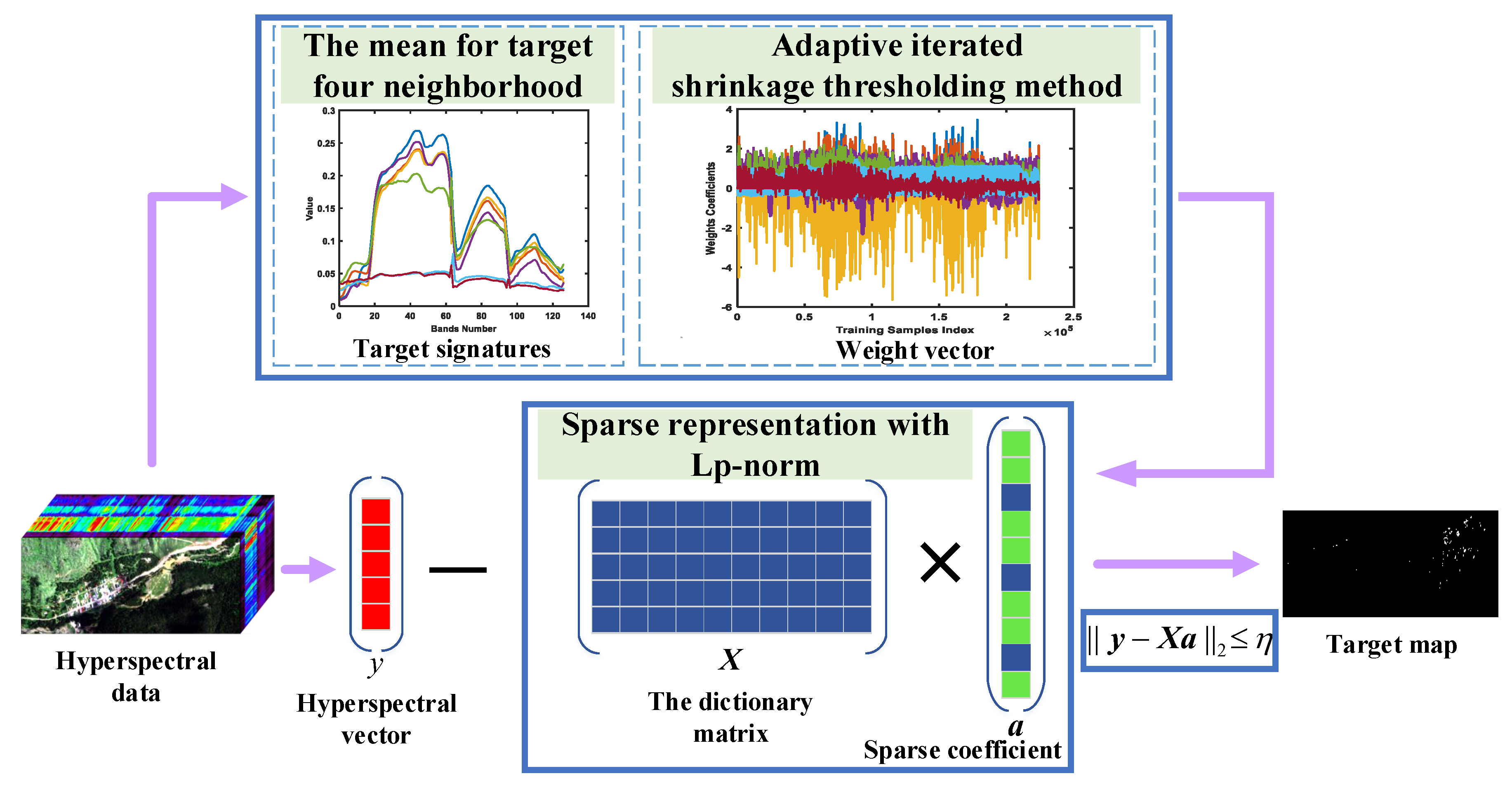
Figure 1. Schematic of the proposed sparse representation with l p -norm framework.
Remotesensing 12 03991 g001
Figure 2. The scenograph of solutions for different norm minimization in 2-D space. (a) The scenograph of the solutions for l 1 -norm minimization. (b) The scenograph of the solutions for l p -norm minimization.
Remotesensing 12 03991 g002
Figure 3. Comparison of l p -norm and l 1 -norm target-based representation residuals of a target pixel (yellow nylon) and a background pixel (mixture of grass and building) in the HyMap data. It is desired that the target pixel has a small residual, and the background pixel has a large residual. (a) Target pixel. (b) Background pixel.
Remotesensing 12 03991 g003
Figure 4. Illustration of the Gulfport dataset: (a) false color (RGB: 60, 30, 20); (b) the ground-truth map.
Remotesensing 12 03991 g004
Figure 5. Illustration of the HyMap dataset: (a) false color (RGB: 60, 30, 20); (b) the ground-truth map.
Remotesensing 12 03991 g005
Figure 6. Illustration of the SpecTIR dataset: (a) false color (RGB: 60, 30, 20); (b) the ground-truth map.
Remotesensing 12 03991 g006
Figure 7. Illustration of the San Diego dataset: (a) false color (RGB: 60, 30, 20); (b) the ground-truth map.
Remotesensing 12 03991 g007
Figure 8. Area under curve (AUC) values of different varying p, as well as lambda ( λ ), in the Gulfport dataset.
Remotesensing 12 03991 g008
Figure 9. AUC values of different varying p, as well as lambda ( λ ), in the HyMap dataset.
Remotesensing 12 03991 g009
Figure 10. AUC values of different varying p, as well as lambda ( λ ), in the SpecTIR dataset.
Remotesensing 12 03991 g010
Figure 11. AUC values of different varying p, as well as lambda ( λ ), in the San Diego dataset.
Remotesensing 12 03991 g011
Figure 12. Detection maps for the Gulfport dataset when p f is fixed to 0.1: (a) Constrained energy minimization (CEM) p d = 0.84. (b) adaptive cosine estimation (ACE) p d = 0.81. (c) matched filter (MF) p d = 0.90. (d) Sparse and Low-Rank Matrix Decomposition (SLMD) p d = 0.98. (e) one-class support vector machine (OC-SVM) p d = 0.95. (f) sparse representation detector (SRD) p d = 0.94. (g) combining sparse and collaborative representations (CSCR) p d = 0.99. (h) l p -norm-based sparse representation detector (Lp-SRD) p d = 1.00.
Remotesensing 12 03991 g012
Figure 13. Detection maps for the HyMap dataset when p f is fixed to 0.15: (a) CEM p d = 0.55. (b) ACE p d = 0.59. (c) MF p d = 0.71. (d) SLMD p d = 0.80. (e) OC-SVM p d = 0.79. (f) SRD p d = 0.86. (g) CSCR p d = 0.62. (h) Lp-SRD p d = 0.94.
Remotesensing 12 03991 g013
Figure 14. Detection maps for the SpecTIR dataset p f is fixed to 0.1: (a) CEM p d = 0.84. (b) ACE p d = 0.72. (c) MF p d = 0.84. (d) SLMD p d = 0.98. (e) OC-SVM p d = 0.79. (f) SRD p d = 0.95. (g) CSCR p d = 0.98. (h) Lp-SRD p d = 1.00.
Remotesensing 12 03991 g014
Figure 15. Detection maps for the San Diego dataset p f is fixed to 0.1: (a) CEM p d = 0.85. (b) ACE p d = 0.72. (c) MF p d = 0.80. (d) SLMD p d = 0.52. (e) OC-SVM p d = 0.90. (f) SRD p d = 0.73. (g) CSCR p d = 0.92. (h) Lp-SRD p d = 1.00.
Remotesensing 12 03991 g015
Figure 16. Detection performance using the Gulfport dataset: (a) Statistical separability analysis. (b) Receiver operate characteristic (ROC) curves.
Remotesensing 12 03991 g016
Figure 17. Detection performance using the HyMap dataset: (a) Statistical separability analysis. (b) ROC curves.
Remotesensing 12 03991 g017
Figure 18. Detection performance using the SpecTIR dataset: (a) Statistical separability analysis. (b) ROC curves.
Remotesensing 12 03991 g018
Figure 19. Detection performance using the San Diego dataset: (a) Statistical separability analysis. (b) ROC curves.
Remotesensing 12 03991 g019
Table 1. AUC values of different target detectors using four experimental datasets.
MethodsCEMACEMFSLMDOC-SVMSRDCSCRLp-SRD
Gulfport0.91540.91840.93710.98710.98520.98480.99080.9960
HyMap0.70820.75540.73590.81820.88350.93030.83930.9468
SpecTIR0.91240.83920.91150.98540.87570.96250.99320.9970
San Diego0.94170.89610.93850.78800.75100.95900.98050.9899
Table 2. Execution time of different target detectors using four experimental datasets (unit: seconds).
MethodsCEMACEMFSLMDOC-SVMSRDCSCRLp-SRD
Gulfport0.11320.15380.10046.64810.06600.82323.02660.8816
HyMap0.17150.36470.22366.59670.24232.338117.90004.8677
SpecTIR0.19050.36880.25077.39710.10512.08568.09122.1889
San Diego0.29160.61210.435212.24670.15222.885511.87673.6604
Publisher’s Note: MDPI stays neutral with regard to jurisdictional claims in published maps and institutional affiliations.