Adaptive-SFSDAF for Spatiotemporal Image Fusion that Selectively Uses Class Abundance Change Information

 ,
,
Abstract
1. Introduction
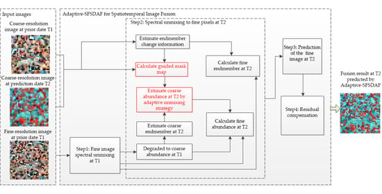
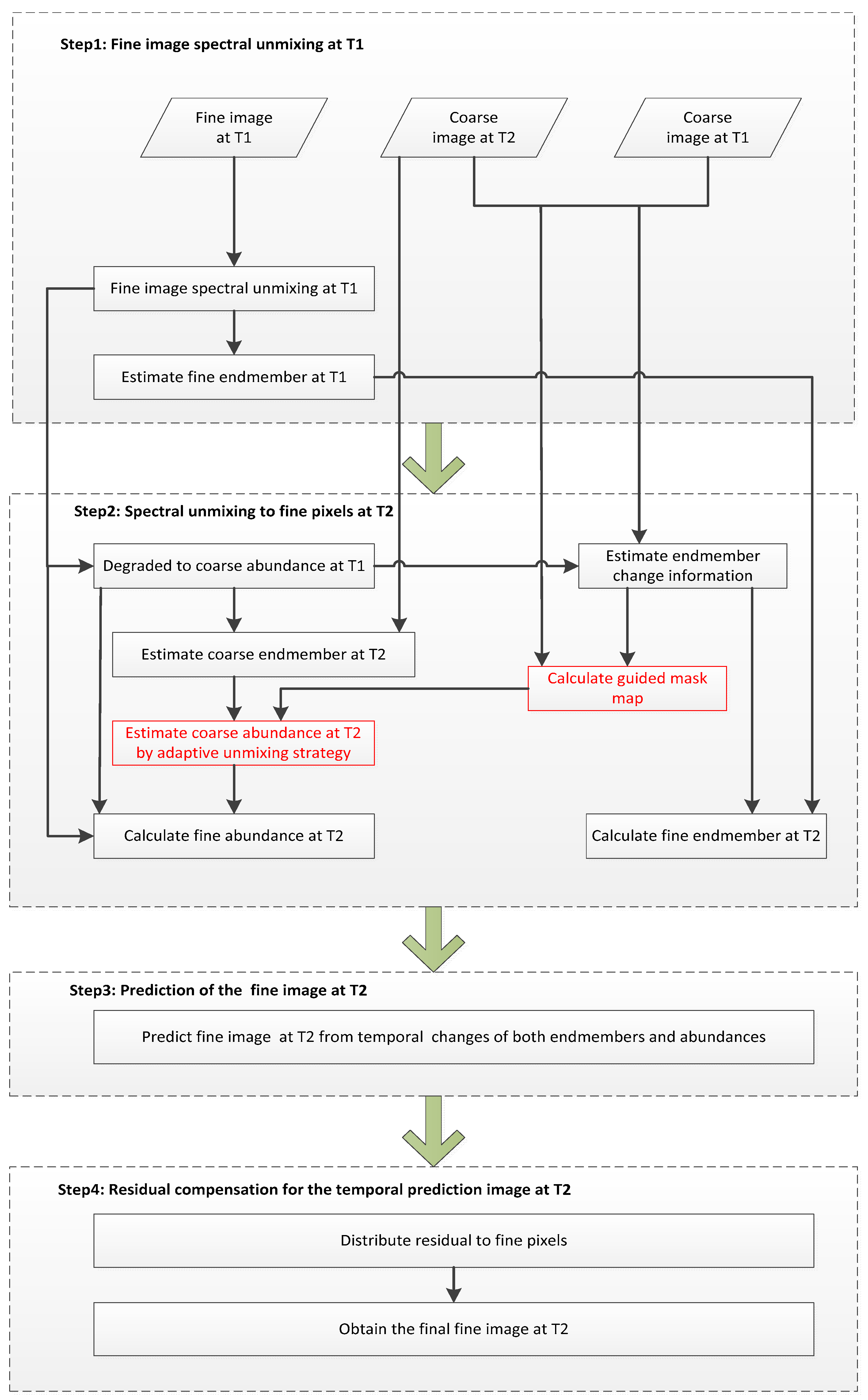
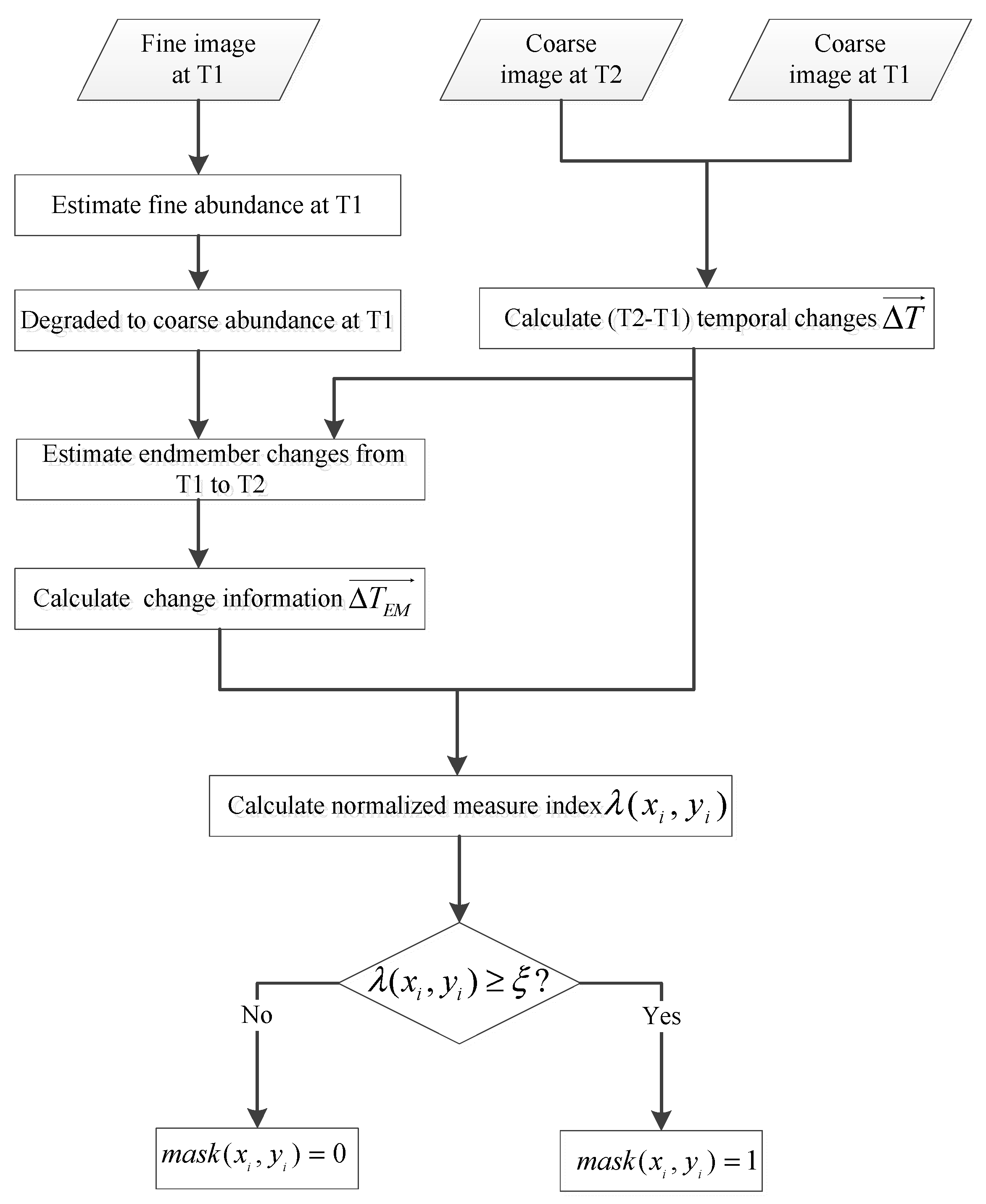
2. Methods
2.1. Fine Image Spectral Unmixing at T1
2.2. Spectral Unmixing to Fine Pixels at T2
2.2.1. Estimation of the Coarse-Resolution Endmember at T2
2.2.2. Estimation of the Fine-Resolution Endmember at T2
2.2.3. Estimation of the Coarse-Resolution Abundance at T2
2.2.4. Estimation of the Fine-Resolution Abundance at T2
2.3. Prediction of the Fine Image at T2
2.4. Residual Compensation for the Temporal Prediction Image at T2
3. Experiments
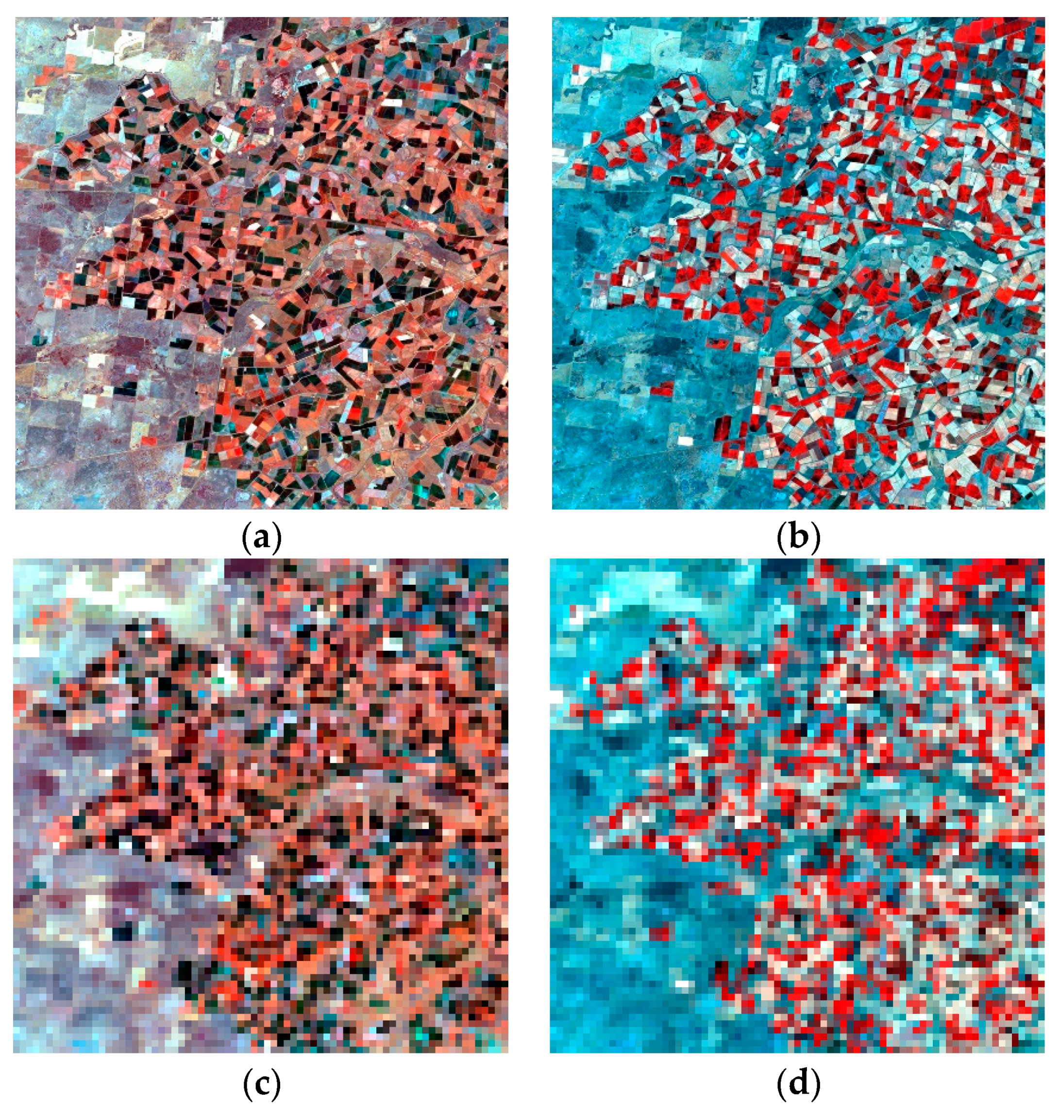
3.1. Study Area and Data
3.2. Comparison and Evaluation
4. Results
4.1. Test Using the Coleambally Dataset with a Heterogeneous Landscape
4.2. Test Using the Gwydir Dataset with Land Cover Type Change
4.3. Comparison of Computation Times
5. Discussion
5.1. Comparison of Adaptive-SFSDAF and SFSDAF for Spatially Heterogeneous Landscapes
5.2. Comparison of Adaptive-SFSDAF and SFSDAF for Landscapes with Land Cover Type Change
6. Conclusions
Author Contributions
Funding
Acknowledgments
Conflicts of Interest
Abbreviations
| K | denotes the number of classes |
| N | denotes the number of selected coarse pixels |
| l | denotes the number of bands |
| t1 | denotes the observation date T1 |
| t2 | denotes the observation date T2 |
| ξ | denotes the mask generation threshold |
| n | denotes the total number of similar pixels |
| C(xi,yi,t1) | denotes the ith coarse pixel value at T1 |
| C(xi,yi,t2) | denotes the ith coarse pixel value at T2 |
| ∆F (c) | denotes the cth endmember change information from T1 to T2 |
| ∆FT | denotes the estimated temporal change information from T1 to T2 |
| ∆T(xi,yi,b) | denotes the ith difference value between C(xi,yi,t2) and C(xi,yi,t1) in band b |
| denotes the ith difference vector between C(xi,yi,t2) and C(xi,yi,t1) | |
| denotes the ith estimated temporal change due to endmember change from T1 to T2 | |
| λ(xi,yi) | denotes the ith normalized measure index, which ranges from 0 to 1 |
| mask(xi,yi) | denotes the ith binary mask value |
References
- Gao, F.; Masek, J.; Schwaller, M.; Hall, F. On the blending of the Landsat and MODIS surface reflectance: Predicting daily Landsat surface reflectance. IEEE Trans. Geosci. Remote Sens. 2006, 44, 2207–2218. [Google Scholar] [CrossRef]
- Mitchell, A.L.; Rosenqvist, A.; Mora, B. Current remote sensing approaches to monitoring forest degradation in support of countries measurement, reporting and verification (MRV) systems for REDD+. Carbon Balance Manag. 2017, 12, 9. [Google Scholar] [CrossRef] [PubMed]
- Hilker, T.; Wulder, M.A.; Coops, N.C.; Linke, J.; McDermid, G.; Masek, J.G.; Gao, F.; White, J.C. A new data fusion model for high spatial- and temporal-resolution mapping of forest disturbance based on Landsat and MODIS. Remote Sens. Environ. 2009, 113, 1613–1627. [Google Scholar] [CrossRef]
- Rogan, J.; Chen, D. Remote sensing technology for mapping and monitoring land-cover and land-use change. Prog. Plan. 2004, 61, 301–325. [Google Scholar] [CrossRef]
- Zhang, J.; Zhou, C.; Xu, K.; Masataka, W. Flood disaster monitoring and evaluation in china. Glob. Environ. Chang. Part B Environ. Hazards 2002, 4, 33–43. [Google Scholar] [CrossRef]
- Joyce, K.E.; Belliss, S.E.; Samsonov, S.V.; McNeill, S.J.; Glassey, P.J. A review of the status of satellite remote sensing and image processing techniques for mapping natural hazards and disasters. Prog. Phys. Geogr. 2009, 33, 183–207. [Google Scholar] [CrossRef]
- Malingreau, J.P. Remote sensing and disaster monitoring—A review of applications in Indonesia. In Proceedings of the 18th International Symposium on Remote Sensing of Environment, Paris, France, 1–5 October 1984; pp. 283–297. [Google Scholar]
- Belgiu, M.; Stein, A. Spatiotemporal image fusion in remote sensing. Remote Sens. 2019, 11, 818. [Google Scholar] [CrossRef]
- Wang, Q.; Atkinson, P.M. Spatio-temporal fusion for daily Sentinel-2 images. Remote Sens. Environ. 2018, 204, 31–42. [Google Scholar] [CrossRef]
- Chen, B.; Huang, B.; Xu, B. Comparison of spatiotemporal fusion models: A review. Remote Sens. 2015, 7, 1798–1835. [Google Scholar] [CrossRef]
- Zhu, X.; Helmer, E.H.; Gao, F.; Liu, D.; Chen, J.; Lefsky, M.A. A flexible spatiotemporal method for fusing satellite images with different resolutions. Remote Sens. Environ. 2016, 172, 165–177. [Google Scholar] [CrossRef]
- Zhong, D.; Zhou, F. A Prediction Smooth Method for Blending Landsat and Moderate Resolution Imagine Spectroradiometer Images. Remote Sens. 2018, 10, 1371. [Google Scholar] [CrossRef]
- Zhong, D.; Zhou, F. Improvement of clustering methods for modelling abrupt land surface changes in satellite image fusions. Remote Sens. 2019, 11, 1759. [Google Scholar] [CrossRef]
- Huang, B.; Zhang, H. Spatio-temporal reflectance fusion via unmixing: Accounting for both phenological and land-cover changes. Int. J. Remote Sens. 2014, 35, 6213–6233. [Google Scholar] [CrossRef]
- Zhao, Y.; Huang, B.; Song, H. A robust adaptive spatial and temporal image fusion model for complex land surface changes. Remote Sens. Environ. 2018, 208, 42–62. [Google Scholar] [CrossRef]
- Wang, J.; Huang, B. A rigorously-weighted spatiotemporal fusion model with uncertainty analysis. Remote Sens. 2017, 9, 990. [Google Scholar] [CrossRef]
- Wu, B.; Huang, B.; Cao, K.; Zhuo, G. Improving spatiotemporal reflectance fusion using image inpainting and steering kernel regression techniques. Int. J. Remote Sens. 2016, 38, 706–727. [Google Scholar] [CrossRef]
- Kwan, C.; Budavari, B.; Gao, F.; Zhu, X. A hybrid color mapping approach to fusing MODIS and Landsat images for forward prediction. Remote Sens. 2018, 10, 520. [Google Scholar] [CrossRef]
- Kwan, C.; Zhu, X.; Gao, F.; Chou, B.; Perez, D.; Li, J.; Shen, Y.; Koperski, K.; Marchisio, G. Assessment of spatiotemporal fusion algorithms for planet and worldview images. Sensors 2018, 18, 1051. [Google Scholar] [CrossRef]
- Liu, M.; Ke, Y.; Yin, Q.; Chen, X.; Im, J. Comparison of five spatio-temporal satellite image fusion models over landscapes with various spatial heterogeneity and temporal variation. Remote Sens. 2019, 11, 2612. [Google Scholar] [CrossRef]
- Zhu, X.; Chen, J.; Gao, F.; Chen, X.; Masek, J.G. An enhanced spatial and temporal adaptive reflectance fusion model for complex heterogeneous regions. Remote Sens. Environ. 2010, 114, 2610–2623. [Google Scholar] [CrossRef]
- Chen, B.; Chen, L.; Huang, B.; Michishita, R.; Xu, B. Dynamic monitoring of the Poyang Lake wetland by integrating Landsat and MODIS observations. ISPRS J. Photogramm. Remote Sens. 2018, 139, 75–87. [Google Scholar] [CrossRef]
- Emelyanova, I.V.; McVicar, T.R.; Van Niel, T.G.; Li, L.T.; van Dijk, A.I. Assessing the accuracy of blending Landsat–MODIS surface reflectances in two landscapes with contrasting spatial and temporal dynamics: A framework for algorithm selection. Remote Sens. Environ. 2013, 133, 193–209. [Google Scholar] [CrossRef]
- Bioucas-Dias, J.M.; Plaza, A.; Dobigeon, N.; Parente, M.; Du, Q.; Member, S.; Chanussot, J. Hyperspectral unmixing overview: Geometrical, statistical, and sparse regression-based approaches. IEEE J. Sel. Top. Appl. Earth Obs. Remote Sens. 2012, 5, 354–379. [Google Scholar] [CrossRef]
- Amorós-López, J.; Gómez-Chova, L.; Alonso, L.; Guanter, L.; Zurita-Milla, R.; Moreno, J.; Camps-Valls, G. Multitemporal fusion of Landsat/TM and ENVISAT/MERIS for crop monitoring. Int. J. Appl. Earth Obs. Geoinf. 2013, 23, 132–141. [Google Scholar] [CrossRef]
- Zhukov, B.; Oertel, D.; Lanzl, F.; Reinhäckel, G. Unmixing-based multisensory multiresolution image fusion. IEEE Trans. Geosci. Remote Sens. 1999, 37, 1212–1226. [Google Scholar] [CrossRef]
- Zurita-Milla, R.; Clevers, J.G.; Schaepman, M.E. Unmixing-based Landsat TM and MERIS FR data fusion. IEEE Geosci. Remote Sens. Lett. 2008, 5, 453–457. [Google Scholar] [CrossRef]
- Zurita-Milla, R.; Kaiser, G.; Clevers, J.; Schneider, W.; Schaepman, M. Downscaling time series of MERIS full resolution data to monitor vegetation seasonal dynamics. Remote Sens. Environ. 2009, 113, 1874–1885. [Google Scholar] [CrossRef]
- Gevaert, C.M.; García-Haro, F.J. A comparison of STARFM and an unmixing-based algorithm for Landsat and MODIS data fusion. Remote Sens. Environ. 2015, 156, 34–44. [Google Scholar] [CrossRef]
- Ma, J.; Zhang, W.; Andrea, M.; Gao, L.; Zhang, B. An Improved Spatial and Temporal Reflectance Unmixing Model to Synthesize Time Series of Landsat-Like Images. Remote Sens. 2018, 10, 1388. [Google Scholar] [CrossRef]
- Xue, J.; Leung, Y.; Fung, T. An Unmixing-Based Bayesian Model for Spatio-Temporal Satellite Image Fusion in Heterogeneous Landscapes. Remote Sens. 2019, 11, 324. [Google Scholar] [CrossRef]
- Xue, J.; Leung, Y.; Fung, T. A bayesian data fusion approach to spatio-temporal fusion of remotely sensedimages. Remote Sens. 2017, 9, 1310. [Google Scholar] [CrossRef]
- Huang, B.; Song, H. Spatiotemporal reflectance fusion via sparse representation. IEEE Trans. Geosci. Remote Sens. 2012, 50, 3707–3716. [Google Scholar] [CrossRef]
- Song, H.; Huang, B. Spatiotemporal satellite image fusion through one-pair image learning. IEEE Trans. Geosci. Remote Sens. 2013, 51, 1883–1896. [Google Scholar] [CrossRef]
- Liu, X.; Deng, C.; Wang, S.; Huang, G.-B.; Zhao, B.; Lauren, P. Fast and accurate spatiotemporal fusion based upon extreme learning machine. IEEE Geosci. Remote Sens. Lett. 2016, 13, 2039–2043. [Google Scholar] [CrossRef]
- Liu, X.; Deng, C.; Chanussot, J.; Hong, D.; Zhao, B. StfNet: A Two-Stream Convolutional Neural Network for Spatiotemporal Image Fusion. IEEE Trans. Geosci. Remote Sens. 2019, 57, 6552–6564. [Google Scholar] [CrossRef]
- Tan, Z.; Yue, P.; Di, L.; Tang, J.J.R.S. Deriving high spatiotemporal remote sensing images using deep convolutional network. Remote Sens. 2018, 10, 1066. [Google Scholar] [CrossRef]
- Song, H.; Liu, Q.; Wang, G.; Hang, R.; Huang, B. Spatiotemporal Satellite Image Fusion Using Deep Convolutional Neural Networks. IEEE J. Sel. Top. Appl. Earth Obs. Remote Sens. 2018, 11, 821–829. [Google Scholar] [CrossRef]
- Li, X.; Foody, G.M.; Boyd, D.S.; Ge, Y.; Zhang, Y.; Du, Y.; Ling, F. Sfsdaf: An enhanced fsdaf that incorporates sub-pixel class fraction change information for spatio-temporal image fusion. Remote Sens. Environ. 2019, 237. [Google Scholar] [CrossRef]
- Ball, G.H.; Hall, D.J. ISODATA, A Novel Method of Data Analysis and Pattern Classification; Technical Report; Stanford Research Institute: Menlo Park, CA, USA, May 1965. [Google Scholar]
- Gao, F.; Hilker, T.; Zhu, X.; Anderson, M.A.; Masek, J.; Wang, P.; Yang, Y. Fusing Landsat and MODIS data for vegetation monitoring. IEEE Geosci. Remote Sens. Mag. 2015, 3, 47–60. [Google Scholar] [CrossRef]
- Quan, J. Blending multi-spatiotemporal resolution land surface temperatures over hetero-geneous surfaces. In Proceedings of the 2017 Joint Urban Remote Sensing Event (JURSE), Dubai, UAE, 6–8 March 2017. [Google Scholar] [CrossRef]


| T1 | UBDF | FIT-FC | FSDAF | SFSDAF | Adaptive-SFSDAF | ||
|---|---|---|---|---|---|---|---|
| RMSE | Band1 | 0.0258 | 0.0172 | 0.0151 | 0.0118 | 0.0113 | 0.0116 |
| Band2 | 0.041 | 0.0277 | 0.0226 | 0.0179 | 0.0169 | 0.0175 | |
| Band3 | 0.0617 | 0.0469 | 0.0352 | 0.0283 | 0.0264 | 0.0275 | |
| Band4 | 0.1152 | 0.0557 | 0.0438 | 0.036 | 0.0354 | 0.0355 | |
| Band5 | 0.0802 | 0.0519 | 0.0415 | 0.0357 | 0.0344 | 0.0354 | |
| Band7 | 0.0541 | 0.041 | 0.0336 | 0.0292 | 0.0284 | 0.029 | |
| MAD | Band1 | 0.0204 | 0.0122 | 0.0107 | 0.0082 | 0.0079 | 0.0082 |
| Band2 | 0.0321 | 0.0196 | 0.0159 | 0.0123 | 0.0117 | 0.0123 | |
| Band3 | 0.0482 | 0.0324 | 0.0242 | 0.0191 | 0.0179 | 0.0188 | |
| Band4 | 0.0805 | 0.0414 | 0.0312 | 0.0247 | 0.0245 | 0.0247 | |
| Band5 | 0.0626 | 0.0368 | 0.0289 | 0.0244 | 0.0234 | 0.0242 | |
| Band7 | 0.0409 | 0.029 | 0.0233 | 0.0196 | 0.0191 | 0.0195 | |
| CC | Band1 | 0.6586 | 0.7869 | 0.8368 | 0.9036 | 0.9128 | 0.9082 |
| Band2 | 0.6427 | 0.7508 | 0.8345 | 0.9006 | 0.9119 | 0.9057 | |
| Band3 | 0.731 | 0.7702 | 0.8732 | 0.9194 | 0.9305 | 0.9246 | |
| Band4 | 0.0898 | 0.5633 | 0.7481 | 0.8379 | 0.8442 | 0.8427 | |
| Band5 | 0.8463 | 0.8585 | 0.9102 | 0.9339 | 0.939 | 0.9356 | |
| Band7 | 0.8694 | 0.8849 | 0.9237 | 0.9427 | 0.9459 | 0.944 | |
| SSIM | Band1 | 0.8629 | 0.8824 | 0.9053 | 0.9234 | 0.9275 | 0.9239 |
| Band2 | 0.8365 | 0.8079 | 0.869 | 0.8832 | 0.891 | 0.8863 | |
| Band3 | 0.7655 | 0.6914 | 0.7906 | 0.8122 | 0.8266 | 0.8173 | |
| Band4 | 0.6321 | 0.6231 | 0.7145 | 0.7488 | 0.7561 | 0.7544 | |
| Band5 | 0.6994 | 0.6823 | 0.7702 | 0.7689 | 0.7814 | 0.7763 | |
| Band7 | 0.7529 | 0.7298 | 0.8026 | 0.8062 | 0.8134 | 0.8103 | |
| PSNR | Band1 | 31.7545 | 35.2938 | 36.4347 | 38.5496 | 38.954 | 38.7268 |
| Band2 | 27.748 | 31.1607 | 32.903 | 34.9645 | 35.4478 | 35.149 | |
| Band3 | 24.2001 | 26.5832 | 29.0748 | 30.9549 | 31.5601 | 31.2184 | |
| Band4 | 18.7718 | 25.0879 | 27.1724 | 28.8701 | 29.0257 | 28.9879 | |
| Band5 | 21.9126 | 25.6997 | 27.6463 | 28.9346 | 29.2691 | 29.0167 | |
| Band7 | 25.3384 | 27.7344 | 29.4774 | 30.6877 | 30.9286 | 30.7642 |
| T1 | UBDF | FIT-FC | FSDAF | SFSDAF | Adaptive-SFSDAF | ||
|---|---|---|---|---|---|---|---|
| RMSE | Band1 | 0.0295 | 0.0152 | 0.0115 | 0.0101 | 0.0098 | 0.0099 |
| Band2 | 0.039 | 0.0222 | 0.017 | 0.0145 | 0.014 | 0.014 | |
| Band3 | 0.0508 | 0.0273 | 0.0207 | 0.0175 | 0.017 | 0.017 | |
| Band4 | 0.0792 | 0.0524 | 0.0331 | 0.0289 | 0.028 | 0.0278 | |
| Band5 | 0.1737 | 0.063 | 0.0508 | 0.0444 | 0.0436 | 0.0437 | |
| Band7 | 0.1385 | 0.0444 | 0.0354 | 0.0316 | 0.0313 | 0.0311 | |
| MAD | Band1 | 0.0256 | 0.0107 | 0.0079 | 0.0073 | 0.0071 | 0.0072 |
| Band2 | 0.0335 | 0.0156 | 0.0117 | 0.0103 | 0.01 | 0.01 | |
| Band3 | 0.0445 | 0.0189 | 0.014 | 0.0123 | 0.0119 | 0.0119 | |
| Band4 | 0.0636 | 0.0391 | 0.0242 | 0.0212 | 0.0204 | 0.0204 | |
| Band5 | 0.1516 | 0.048 | 0.0371 | 0.0331 | 0.0324 | 0.0327 | |
| Band7 | 0.1243 | 0.033 | 0.0255 | 0.0231 | 0.0228 | 0.0227 | |
| CC | Band1 | 0.3881 | 0.6563 | 0.8185 | 0.8627 | 0.8702 | 0.8684 |
| Band2 | 0.3382 | 0.6523 | 0.8096 | 0.8662 | 0.8749 | 0.8746 | |
| Band3 | 0.3871 | 0.6531 | 0.8142 | 0.8705 | 0.8801 | 0.8793 | |
| Band4 | 0.4963 | 0.5898 | 0.8495 | 0.8877 | 0.895 | 0.8971 | |
| Band5 | 0.2927 | 0.5931 | 0.7564 | 0.8192 | 0.8273 | 0.8278 | |
| Band7 | 0.4002 | 0.586 | 0.7595 | 0.8149 | 0.8212 | 0.8238 | |
| SSIM | Band1 | 0.8425 | 0.9093 | 0.9397 | 0.9437 | 0.947 | 0.9463 |
| Band2 | 0.8225 | 0.8575 | 0.8987 | 0.9095 | 0.9156 | 0.9157 | |
| Band3 | 0.7784 | 0.8194 | 0.8712 | 0.8851 | 0.8941 | 0.8937 | |
| Band4 | 0.7109 | 0.6064 | 0.7735 | 0.7903 | 0.8043 | 0.8119 | |
| Band5 | 0.4178 | 0.5096 | 0.5956 | 0.62 | 0.6347 | 0.6391 | |
| Band7 | 0.4229 | 0.6029 | 0.6857 | 0.7068 | 0.7198 | 0.723 | |
| PSNR | Band1 | 30.5947 | 36.3693 | 38.8205 | 39.9448 | 40.1689 | 40.1124 |
| Band2 | 28.1789 | 33.08 | 35.3827 | 36.8026 | 37.0646 | 37.05 | |
| Band3 | 25.8912 | 31.2827 | 33.6768 | 35.1207 | 35.4151 | 35.3817 | |
| Band4 | 22.0276 | 25.6164 | 29.6146 | 30.7911 | 31.0706 | 31.1095 | |
| Band5 | 15.2018 | 24.018 | 25.8872 | 27.045 | 27.2041 | 27.1898 | |
| Band7 | 17.1708 | 27.0463 | 29.0097 | 29.9939 | 30.0891 | 30.1437 |
| Example 1 | Example 2 | |||||
|---|---|---|---|---|---|---|
| Total Time | Time of Spectral Unmixing | Number of Unmixed Pixels | Total Time | Time of Spectral Unmixing | Number of Unmixed Pixels | |
| UBDF | 757.1 | - | - | 1572.0 | - | - |
| FIT-FC | 286.2 | - | - | 506.3 | - | - |
| FSDAF | 515.1 | - | - | 948.3 | - | - |
| SFSDAF | 343.2 | 73.3 | 5625 | 574.2 | 89.4 | 10,000 |
| Adaptive-SFSDAF | 286.4 | 14.2 | 1100 | 504.8 | 20.4 | 2295 |
Publisher’s Note: MDPI stays neutral with regard to jurisdictional claims in published maps and institutional affiliations. |
© 2020 by the authors. Licensee MDPI, Basel, Switzerland. This article is an open access article distributed under the terms and conditions of the Creative Commons Attribution (CC BY) license (http://creativecommons.org/licenses/by/4.0/).
Share and Cite
Hou, S.; Sun, W.; Guo, B.; Li, C.; Li, X.; Shao, Y.; Zhang, J. Adaptive-SFSDAF for Spatiotemporal Image Fusion that Selectively Uses Class Abundance Change Information. Remote Sens. 2020, 12, 3979. https://doi.org/10.3390/rs12233979
Hou S, Sun W, Guo B, Li C, Li X, Shao Y, Zhang J. Adaptive-SFSDAF for Spatiotemporal Image Fusion that Selectively Uses Class Abundance Change Information. Remote Sensing. 2020; 12(23):3979. https://doi.org/10.3390/rs12233979
Chicago/Turabian StyleHou, Shuwei, Wenfang Sun, Baolong Guo, Cheng Li, Xiaobo Li, Yingzhao Shao, and Jianhua Zhang. 2020. "Adaptive-SFSDAF for Spatiotemporal Image Fusion that Selectively Uses Class Abundance Change Information" Remote Sensing 12, no. 23: 3979. https://doi.org/10.3390/rs12233979
APA StyleHou, S., Sun, W., Guo, B., Li, C., Li, X., Shao, Y., & Zhang, J. (2020). Adaptive-SFSDAF for Spatiotemporal Image Fusion that Selectively Uses Class Abundance Change Information. Remote Sensing, 12(23), 3979. https://doi.org/10.3390/rs12233979