Abstract
Many spatiotemporal image fusion methods in remote sensing have been developed to blend highly resolved spatial images and highly resolved temporal images to solve the problem of a trade-off between the spatial and temporal resolution from a single sensor. Yet, none of the spatiotemporal fusion methods considers how the various temporal changes between different pixels affect the performance of the fusion results; to develop an improved fusion method, these temporal changes need to be integrated into one framework. Adaptive-SFSDAF extends the existing fusion method that incorporates sub-pixel class fraction change information in Flexible Spatiotemporal DAta Fusion (SFSDAF) by modifying spectral unmixing to select spectral unmixing adaptively in order to greatly improve the efficiency of the algorithm. Accordingly, the main contributions of the proposed adaptive-SFSDAF method are twofold. One is to address the detection of outliers of temporal change in the image during the period between the origin and prediction dates, as these pixels are the most difficult to estimate and affect the performance of the spatiotemporal fusion methods. The other primary contribution is to establish an adaptive unmixing strategy according to the guided mask map, thus effectively eliminating a great number of insignificant unmixed pixels. The proposed method is compared with the state-of-the-art Flexible Spatiotemporal DAta Fusion (FSDAF), SFSDAF, FIT-FC, and Unmixing-Based Data Fusion (UBDF) methods, and the fusion accuracy is evaluated both quantitatively and visually. The experimental results show that adaptive-SFSDAF achieves outstanding performance in balancing computational efficiency and the accuracy of the fusion results.
1. Introduction
Earth observation missions have played an important role in coping with global changes and solving many problems and challenges related to the development of human society. Both land cover dynamics monitoring, such as timely crop monitoring [1], forest degradation monitoring [2,3], and land use change detection [4], and emergency response to disaster monitoring [5,6,7], such as forest fire and flood monitoring, require remote sensing data with both high spatial and high temporal resolution. Although high spatial and spectral resolution with frequent coverage are the long-term targets of remote sensors, it is difficult for a single sensor to have both high spatial and temporal resolution due to technological constraints. In addition, cloud and shadow contamination also make a large number of remote sensing images unusable. Over the last decade, increasing numbers of remote sensing satellites have been launched, collecting multi-modal remote sensing data with multi-sensor, multi-resolution, and multi-temporal properties. Therefore, there is an increasing amount of research focused on fusing multi-modal remote sensing data to collect fine-scale data with high spatiotemporal resolution.
Spatiotemporal image fusion approaches in remote sensing have been developed for blending images with fine spatial resolution but coarse temporal resolution (e.g., Landsat imagery) with images with fine temporal resolution but coarse spatial resolution (e.g., MODIS imagery) to generate fine-spatiotemporal-resolution images [8,9,10,11]. With minimal input, given one pair of fine-coarse images acquired on nearly the same day (hereafter referred to as T1,) and one coarse image acquired on the predicted date (hereafter referred to as T2), the output is the fine-spatial-resolution image at T2; this technique can make better use of remote sensing data in Earth observation missions by fully mining the inherent associations of multi-modal remote sensing data.
Spatiotemporal image fusion in remote sensing integrates the super-resolution problem in the temporal, spatial, and spectral domains. In the temporal domain, it is necessary to estimate temporal change information to predict the target image. Thus, many fusion methods using change detection techniques are proposed, such as fusion methods based on two fine-coarse image pairs [3,12,13,14], and fusion methods based on one fine-coarse image pair [15,16,17,18,19]. The Hybrid Color Mapping (HCM) approach [18,19], which directly established the mapping between two MODIS images at different times and then used that mapping for forward prediction, can work well for homogeneous images. In the spatial domain, such a method estimates the predicted image information through the self-similar characteristics in the scene. Such methods are often referred to as weighted function-based methods [20]. The spatial and temporal adaptive reflectance fusion model (STARFM) is the one of the earliest to establish the satellite fusion model [1], which is simple, flexible and the most widely used. However, this method assumes that the land cover type in the coarse pixel does not change over the prediction period, so the performance degrades somewhat when used on landscapes with high heterogeneity. Improved algorithms based on STARFM include the enhanced version of STARFM (ESTARFM) [21] and the Spatio-Temporal Adaptive Fusion model For NDVI products (STAFFN) [22]. Emelyanova et al. [23] compared STARFM and ESTARFM and concluded that ESTARFM achieved better performance where/when spatial variance was dominant; STARFM achieved better performance where/when temporal variance was dominant. The method of retrieving fine image information in the spectral domain is often referred to as an unmixing-based method. The traditional unmixing-based method is based on the linear mixing model to solve the fractional abundance of endmembers [24], but the unmixing based method used in the fusion model is somewhat different. More precisely, it is a spatial unmixing method [25] that estimates the endmembers in the sliding window where the class abundance is known; therefore, spatial unmixing can describe the endmember variability of different spatial regions. One of the earliest unmixing methods is the Multisensor Multiresolution Technique (MMT) [26], and many improved variants have been proposed. Zurita-Milla et al. [27,28] used constrained least squares in the unmixing process to obtain a justified solution. Amorós-López et al. [25] added a regularization term to the cost function to restrict the variance of the endmember spectra. Gevaert and García-Haro [29] proposed the Spatial and Temporal Reflectance Unmixing Model (STRUM) using Bayesian method that describes data fusion uncertainties in a clear probabilistic framework. Based on STRUM, Ma et al. [30] proposed an improved method (ISTRUM) by applying fine-resolution abundance image, which can generate higher accuracy than STRUM. In addition to the above algorithms, there are other fusion approaches that incorporate the unmixing based method to improve the performance of existing algorithms. For example, two improved Bayesian data fusion approaches (ISTBDF-I and -II) [31] were proposed by incorporating an unmixing based algorithm into the existing Spatiotemporal Bayesian Data Fusion (STBDF) framework [32], which can enhance the fusion ability of existing STBDF model in handling heterogeneous areas.
In recent years, due to the development of machine learning and deep learning, many learning-based methods have also been developed, including SPSTFM based on two pairs of input images [33], one pair learning based on sparse representation [34], extreme learning [35], and deep learning [36,37,38]. This type of method learns the correspondence between the available coarse-fine image pairs in a whole framework. For example, the StfNet [36] learns two fine difference images predictions from the corresponding coarse ones at forward and backward dates respectively, and further optimizes the fusion results through a temporal constraint among time-series images. This method is based on two fine-coarse image pairs and is suitable for monitoring intermediate dynamics.
Meanwhile, additional fusion methods use a mixture of multiple technologies introduced previously to achieve higher fusion performance. For example, the Flexible Spatiotemporal DAta Fusion (FSDAF) [11] first estimated the temporal changes of endmembers in a scene based on the spatial unmixing method to describe gradual phenology changes, then used spatial interpolation to characterize sudden land cover type changes, and finally performed residual compensation based on a weighted function of similar pixels.
Based on FSDAF, an enhanced fusion method incorporates sub-pixel class fraction change information in Flexible Spatiotemporal DAta Fusion (SFSDAF) [39], resulting in better performance when applied to landscapes with many mixed pixels and land cover type changes. However, in practice, not all pixels experienced class abundance changes, and SFSDAF still unmixed such pixels with invariant class abundance, which not only leads to a large computational burden, but also brings some uncertainty to the prediction model. There are no spatiotemporal fusion methods that consider the various temporal changes among in different pixels, which can affect the performance of the fusion results, or how these changes could be integrated into one framework to develop an improved fusion method. The adaptive-SFSDAF proposed in this paper is based on SFSDAF, a recently developed, best-performing method with minimal input pairs. Adaptive-SFSDAF first detects outliers in the image over the prediction period and then selectively uses class abundance change information by a guided mask map. The proposed adaptive-SFSDAF optimizes the unchanged-type areas contained in land cover class change more directly from the perspective of class abundance information present in the image, thus reducing the uncertainty in the SFSDAF prediction model. Although Wu et al. [17] also used a changed mask map in the reflectance fusion method, their method is based on the regularized Iteratively Reweighted Multivariate Alteration Detection (IR- MAD) method, and only determines whether a pixel is changed or not. In experiments, our proposed method is compared with the state-of-the-art FSDAF, SFSDAF, FIT-FC, and Unmixing-Based Data Fusion (UBDF) methods, and the fusion accuracy is evaluated both quantitatively and visually. According to the experimental results, the following two conclusions are drawn:
(1) For both Coleambally and Gwydir, adaptive-SFSDAF can greatly reduce the number of unmixed pixels in spectral unmixing processing; nearly 80% of the total pixels are shown to be unnecessary in terms of prediction accuracy and, thus, can be eliminated with negligible loss of performance. This shows that adaptive-SFSDAF can achieve significant unmixed pixels reduction while preserving comparable fusion performance using full unmixed pixels.
(2) Adaptive-SFSDAF reduced the uncertainty in the SFSDAF prediction model by optimizing the unchanged-type areas of land cover class change, thus strengthening the robustness of SFSDAF. In particular, adaptive-SFSDAF was superior when capturing the Gwydir site image structure. For both types of sites, adaptive-SFSDAF achieved better performance than FSDAF, according to both visual and quantitative measurements.
2. Methods
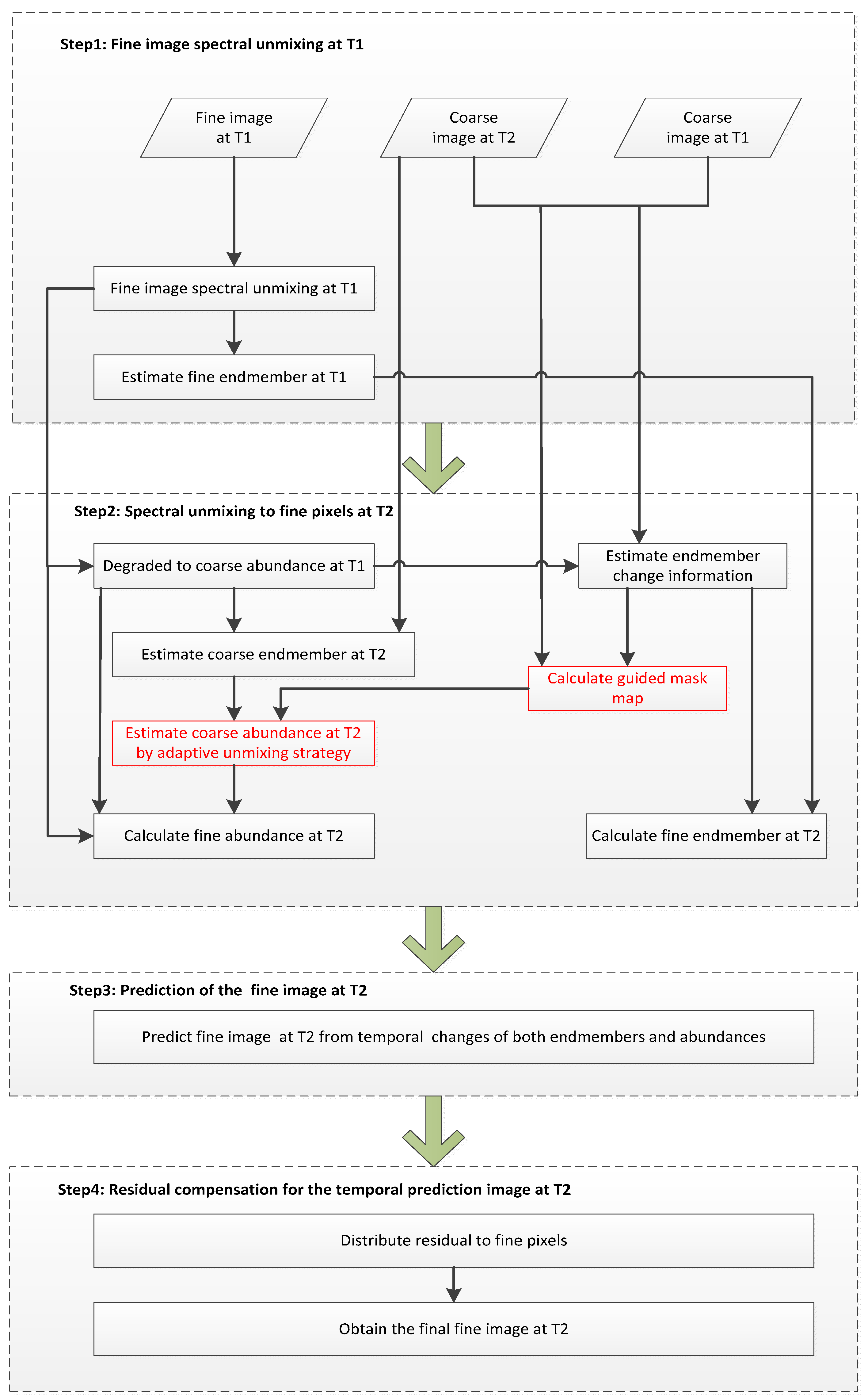
In Adaptive-SFSDAF, a pair of fine-coarse images acquired at T1 and one coarse image acquired at T2 are known. The aim of the fusion algorithm is to predict the fine image corresponding to the coarse input at T2. Because the fine-coarse images are obtained by two different sensors, the input pair needs to be geographically registered first to facilitate subsequent fusion processing [1]. Adaptive-SFSDAF mainly includes the following four steps: (1) spectral unmixing of the fine image at T1 to obtain its endmembers and abundances; (2) estimation of the spectral unmixing result for the fine image at T2; (3) prediction of the fine image at T2 according to the change information of both endmembers and class abundances; and (4) compensation for the prediction residual and production of the final fine image at T2. The flowchart of the proposed adaptive-SFSDAF is shown in Figure 1. In this proposed process, the difference between adaptive-SFSDAF and SFSDAF occurs in step 2, corresponding to the red boxes in Figure 1. Adaptive-SFSDAF is detailed as follows. The notations and definitions in adaptive-SFSDAF are provided in Abbreviations.
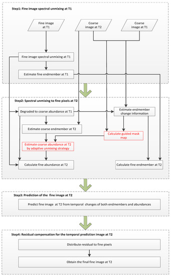
Figure 1.
Flowchart of the proposed adaptive- sub-pixel class fraction change information incorporated in Flexible Spatiotemporal DAta Fusion (SFSDAF).
2.1. Fine Image Spectral Unmixing at T1
First, the fine-resolution (fine) image at T1 is classified by either a supervised or an unsupervised classification method. In order to classify the image automatically, an unsupervised clustering method, such as Iterative Self-Organizing Data Analysis Technique Algorithm (ISODATA), is applied [40]. According to the classification map, endmember information of the image can be estimated using the average vector of each class. Then, the abundance of class at each pixel (xi,yi) can be estimated by soft classification as follows:
where F(xi,yi,t1) is the fine image at observation date T1, (xi,yi) represents the spatial position of each input spectral vector, K is the total number of classes, vc is the average vector of class c; ‖X‖∑ is the Mahalanobis norm, which is calculated by ‖X‖∑=XT∑−1X, and Σ denotes the sample covariance matrix.
After solving the class abundance of the fine image at T1, the endmember information can be estimated according to the well-known linear mixing model (LMM). The endmember rFR(c,b,t1) can be calculated by solving the following equation:
where F(xi,yi,b,t1) is the band b value of the fine image at T1. Equation (2) is solved separately for each band b of l total bands.
2.2. Spectral Unmixing to Fine Pixels at T2
In order to predict the fine image at T2, the temporal change information of the image from T1 to T2 needs to be calculated. FSDAF estimates the time variation of endmembers, while SFSDAF further considers the time variation of abundance information within each fine pixel. Because the fine details at T2 are unknown except for the coarse-resolution (coarse) image, the estimation of the fine abundance map at T2 will use the coarse image at T2 repeatedly. The estimation of the fine abundance map at T2 can be accomplished by the spectral unmixing method. The main steps are detailed as follows.
2.2.1. Estimation of the Coarse-Resolution Endmember at T2
Let C(xi,yi,t1) be the coarse image observed at T1 where (xi,yi) is the ith pixel. Its abundance map can be obtained by downsampling the fine abundance map aFR(xij,yij,c,t1):
where f↓ represents the downsampling operator and aFR(xij,yij,c,t1) denotes the jth fine-resolution abundance value within the ith coarse-resolution abundance value aCR(xi,yi,c,t1) at T1.
Next, the endmember information of the coarse image at T2 can be estimated based on the linear mixing model,
where C(xi,yi,b,t2) is the coarse image of band b observed at T2 and rCR(c,b,t2) is the cth endmember in spectrum b corresponding to the coarse image at T2.
Since the abundance information of the coarse image at T2 is unknown, here the corresponding abundance information at T1 is used for approximation. This approximation error can be reduced using a pixel selection strategy, similar to the method used in [11]. It is worth mentioning that an iterative algorithm that repeatedly estimates rCR(c,b,t2) and updates aCR(xi,yi,c,t2) by Equation (4) and Equation (7) could be a better alternative for situations with no time constraints.
2.2.2. Estimation of the Fine-Resolution Endmember at T2
Assuming that the land cover type does not change between T1 and T2, the temporal change in a coarse pixel at location (xi,yi) in band b can be expressed as follows:
where ∆T(xi,yi,b) is the difference value between C(xi,yi,t2) and C(xi,yi,t1) in band b and ∆F(c,b) is the endmember change information. To avoid the collinearity problem, the purest pixels of each class are selected. At the same time, only pixels with moderate amounts of change are used to avoid the effects of the land cover type change. The final N(N > K) selected pixels can form N linear mixing equations. Then, ∆F(c,b) can be solved using the above equations by the least square method.
The fine-resolution endmember at T2 can be estimated by adding the fine-resolution endmember at T1 and the endmember change information between T1 and T2:
2.2.3. Estimation of the Coarse-Resolution Abundance at T2
According to the coarse-resolution endmember at T2, the corresponding abundance for each coarse pixel at T2 can be solved using the linear unmixing method. Let l be the total band number of the input image; then, l equations can be obtained by the well-known linear mixing model (LMM), the coarse resolution abundance can be derived by the constrained least square method. The formula is as follows:
where aCR(xi,yi,c,t2) is the coarse-resolution abundance value of class c at T2.
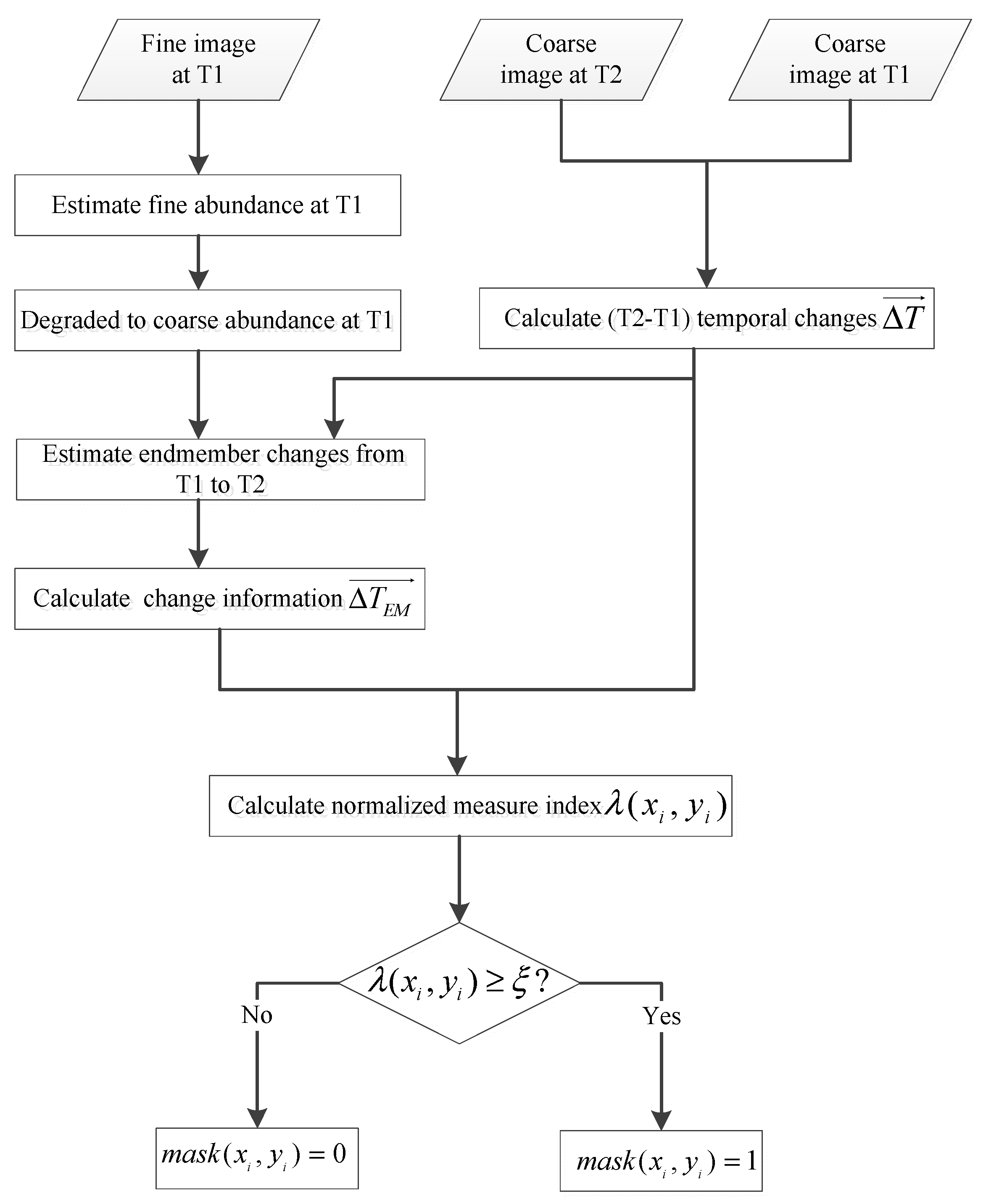
In order to obtain each abundance value at position (xi,yi), SFSDAF needs to solve the above LMM model pixel by pixel, which leads to a large computational burden. Note that the endmember estimation process also needs to solve linear mixture equations, but only once for the whole image. It is apparent that with increases in the size and band number of the input image, the computation time will increase proportionally. This is an intolerable problem for rapid fusion of large remote sensing images. Adaptive-SFSDAF compares the actual change information of the image from T1 to T2 with the predicted endmember change information, and then derives a mask whose pixel value represents whether spectral unmixing is needed. According to the various temporal changes between different pixels over the prediction period, the mask will dynamically select some pixels to guide the spectral unmixing, thus greatly increasing the speed of the unmixing processing by SFSDAF. The mask is explained in the below:
The actual change information of the coarse images from T1 to T2 is defined as:
From the endmember change ∆F, we can derive:
Now, comparing the two change information terms and , the normalized measure index at (xi,yi) is defined as:
The range of the normalized measure index λ(xi,yi) is [0,1]. It can be seen that if and are equal, the minimum value of 0 will be taken, and if the directions of and are opposite, the maximum value of 1 will be chosen.
Let ξ be the mask generation threshold. Using the threshold method for the variable λ(xi,yi), the final binary mask at (xi,yi) is obtained:
Since the value range of λ(xi,yi) is [0,1], the mask generation threshold ξ ranges from 0 to 1 correspondingly. When the maximum value of 1 is taken by ξ, pixels with opposite directions of and are selected for spectral unmixing. When the minimum value of 0 is taken by ξ, then all the pixels are selected for spectral unmixing, and adaptive-SFSDAF is the same as SFSDAF.
A flowchart of the proposed method is shown in Figure 2. When performing the linear unmixing processing of the coarse image at T2, only the pixels where the mask is valid are unmixed:

Figure 2.
Flowchart of the calculation of the guided mask map in adaptive-SFSDAF.
2.2.4. Estimation of the Fine-Resolution Abundance at T2
After solving the abundance information of the coarse image at T1 and T2, the temporal change in the coarse-resolution abundance from T1 to T2 can be obtained as follows:
The corresponding temporal change in the fine-resolution abundance can be obtained by upsampling and refinement processing:
where f↑ is the upsampling operator, B is the weighted function for refinement, and ∆aFR(xij,yij,c) denotes the jth fine-resolution abundance change within the ith coarse-resolution abundance change ∆aCR(xi,yi,c) of class c.
Similar to finding the endmembers of the fine image at T2, the abundance of the fine image at T2 can also be calculated as follows:
2.3. Prediction of the Fine Image at T2
Since the temporal endmember change and abundance change from T1 to T2 are both estimated in the aforementioned steps, the fine image at T2 can be predicted:
where FTP(xi,yi,t2) is referred to as the temporal prediction image because it combines the fine image at T1 and the temporal change information ∆FT. Within the temporal change information, each pixel is modeled as a linear mixture of material endmembers in the image. By respectively representing the fine pixel at T1 and T2 using the LMM model, the temporal change information can be derived accordingly. The advantage of using temporal change information to predict the target is that the two known coarse images can be fully utilized, and more importantly, except for the temporal change information, there is no need to consider the reconstruction accuracy of any image.
2.4. Residual Compensation for the Temporal Prediction Image at T2
Residuals exist in the whole processing chain and, thus, residual compensation is needed to refine the obtained predicted image. Let RCR(xi,yi) be the coarse-resolution residuals at (xi,yi). The coarse-resolution temporal change is defined as:
Then, we obtain
Since the real fine image at T2 is unknown, only coarse-resolution residuals can be calculated from the known conditions. To compensate for these residuals in order to produce the fine prediction image, the key problem is to derive the fine-resolution residuals from its corresponding coarse-resolution residuals.
For a single coarse pixel, the aim is to allocate the residuals to each fine pixel inside it. Since the coarse image at T2 is the only information known at that time, its spatial interpolation can produce another spatial predicted image. Combined with the local uniformity characteristics of the pixel, the allocation weight can be estimated. Let RFR(xij,yij) be the fine residuals at location (xij,yij), which is calculated as:
where w(ij,ij) is the allocated weight at fine pixel (ij,ij) inside the coarse pixel at location (xi,yi).
After residual compensation the fine predicted image at T2 is:
Since the residual distribution is allocated within each coarse pixel, the distributed image will have obvious coarse-grained effect at the edge of each coarse pixel. In order to overcome this problem and maintain the spectral characteristics of the original image, further refinement process is implemented using spectrally similar pixels within the neighborhood of target pixel (xij,yij):
where n is the total number of similar pixels and wk is the weight of the similar pixel k.
3. Experiments
3.1. Study Area and Data
Two sets of images in this study were used for testing the proposed method. The fine images are real Landsat remote sensing data from public remote sensing datasets provided by Dr. Emelyanova et al. [23]. In order to avoid the influence of radiometric and geometric inconsistencies from different sensors on the fusion algorithms, degraded MODIS-like images were used as coarse images, which is a commonly used strategy in performance comparison of spatiotemporal satellite image fusion models [11]. In all of the experiments, the degrading factor was 16. Six spectral bands were used: red, green, blue, infrared, and two shortwave infrared bands.
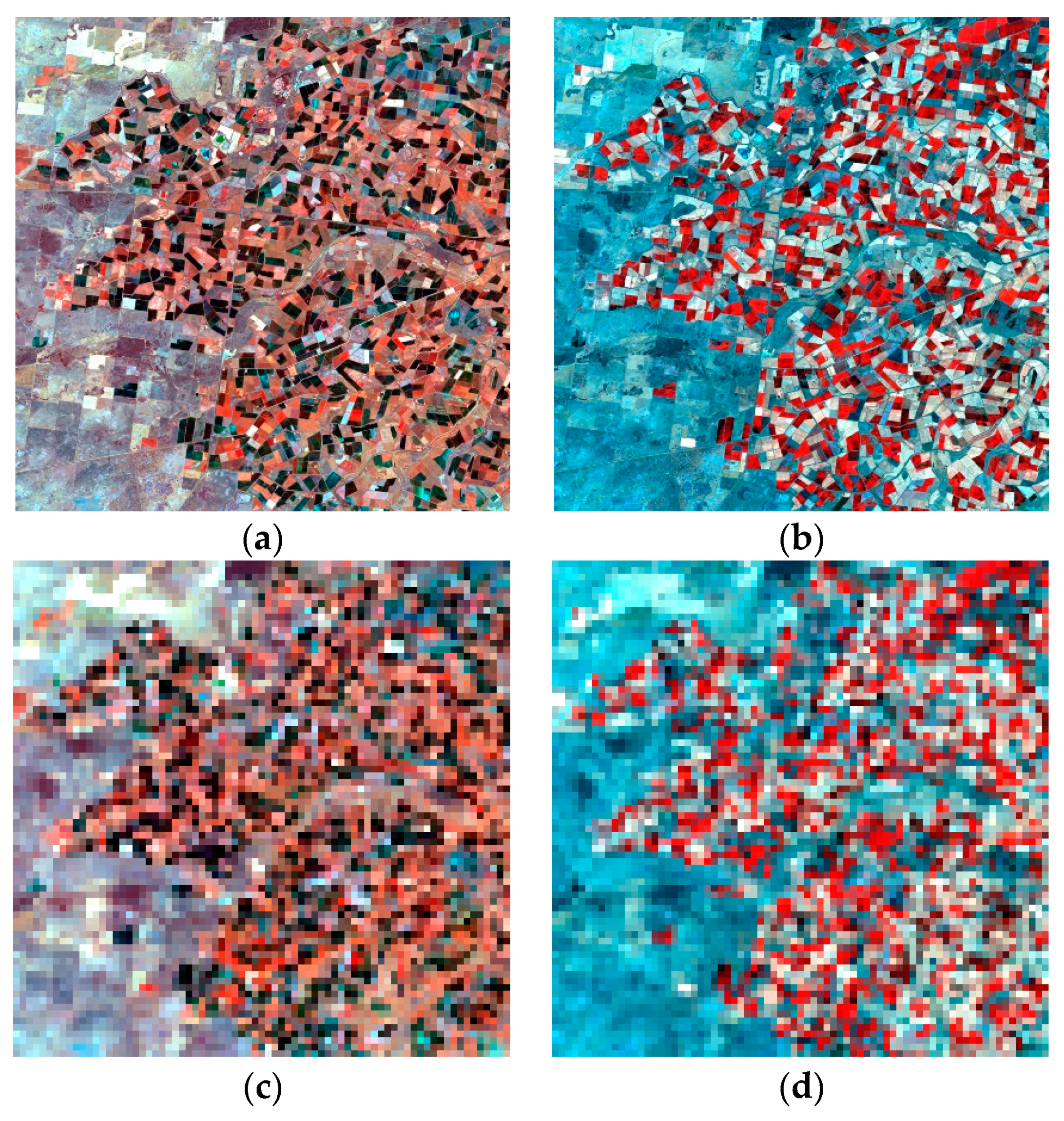
The first set of data come from the Coleambally Irrigation Area (Coleambally), which is located in southern New South Wales of Australia (34.0034 E, 145.0675 S). This region is planted with a variety of different crops. These scattered, small, patchy crops show a complicated distribution with heterogeneous characteristics. The Landsat images were acquired on 25 December 2001 (T1), and 12 January 2002 (T2). Figure 3a,b show the fine images at T1 and T2, which have a size of 1200 × 1200 and a spatial resolution of 25 m. Figure 3c,d are the corresponding degraded MODIS-like images. Coleambally mainly consists of irrigated rice crops and other farmlands. It can be seen that this period happens to be the austral summer growing season, which leads to obvious temporal changes. The input to the spatiotemporal fusion algorithm is the pair of images taken on 25 December 2001 (Figure 3a,c at T1), and the coarse image taken on 12 January 2002 (Figure 3d at T2). The output is the predicted fine image at T2 based on the three available images. Figure 3b presents the evaluation reference image for the predicted image at T2.
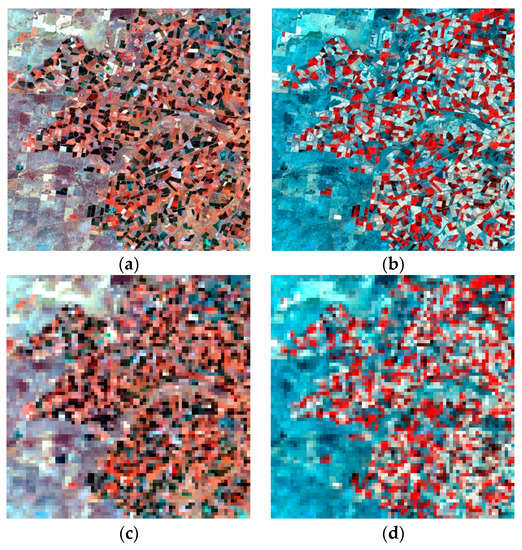
Figure 3.
Dataset of Coleambally: real Landsat-7 images acquired on 25 December 2001 (a), and 12 January 2002 (b), (c,d) are simulated MODIS-like images with a degrading factor 16.
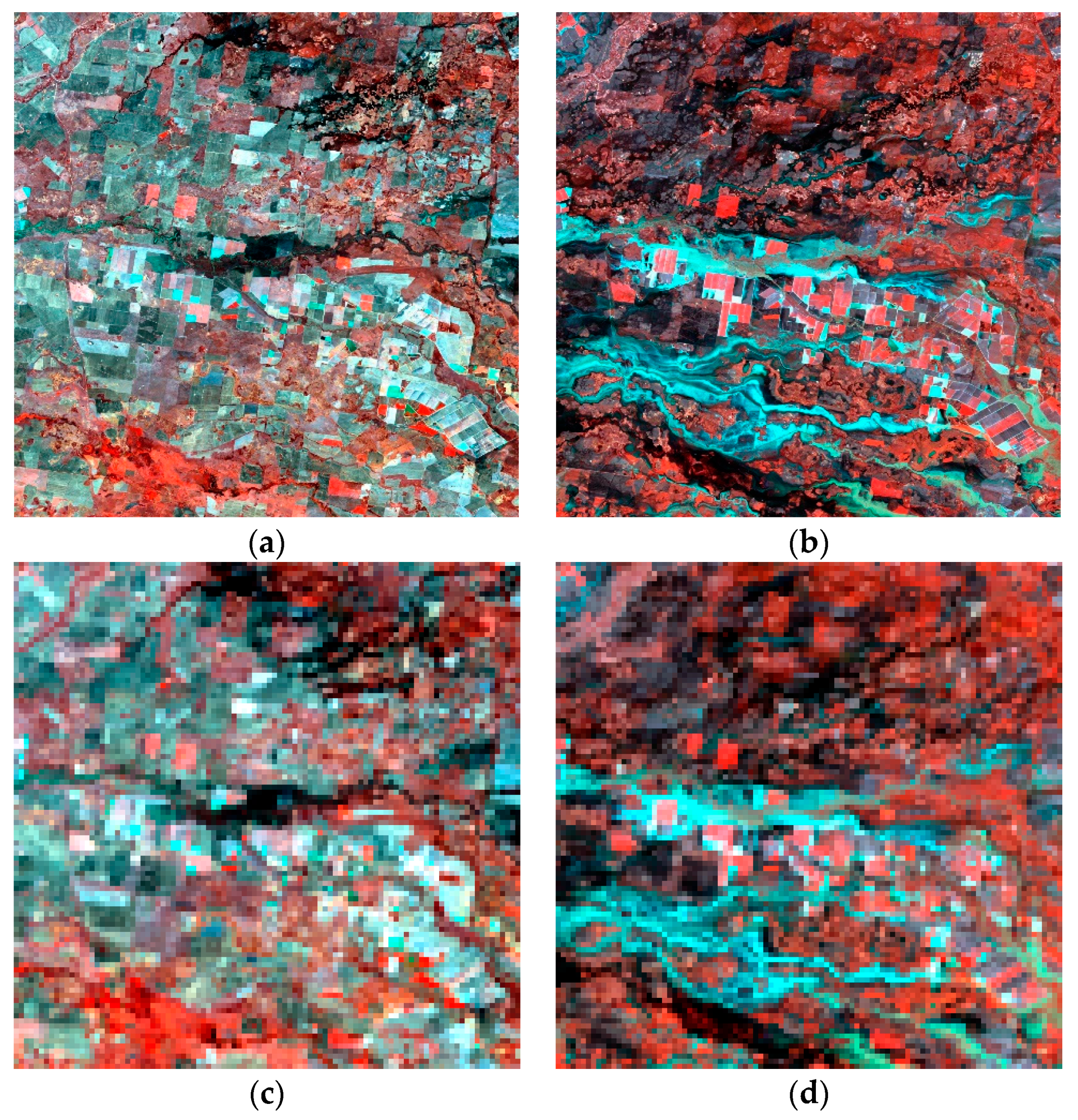
The second set of data comes from the Lower Gwydir Catchment (“Gwydir”) located in northern New South Wales of Australia (149.2815 E, 29.0855 S). This site is representative of dramatic temporal change because of a large flooding event that occurred in mid-December 2004. The Landsat images were acquired on 26 November 2004 (T1), and 12 December 2004 (T2). Figure 4a,b show the fine images at T1 and T2, which have a size of 1600 × 1600 and a spatial resolution of 25 m. Figure 4c,d are the corresponding degraded MODIS-like images. It can be seen that many areas at T1 change to large, water-inundated areas at T2 due to the sudden flooding. Different from that in Coleambally, the large temporal change of Gwydir mainly can be attributed to the land cover type change. The input to the spatiotemporal fusion algorithm is the pair of images taken on 26 November 2004 (Figure 4a,c at T1), and the coarse image taken on 12 December 2004 (Figure 4d at T2). The output is the predicted fine image at T2 based on the three available images. Figure 4b is the reference image for the predicted image at T2.
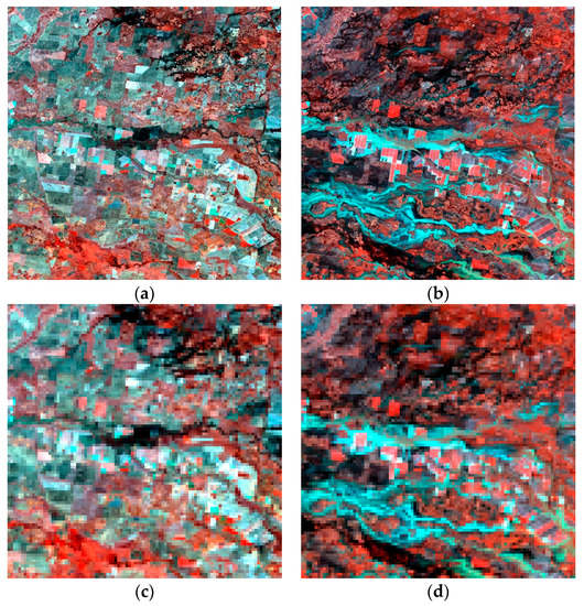
Figure 4.
Dataset of Gwydir: real Landsat-5 acquired on 26 November 2004 (a), and 12 December 2004 (b,c) and (d) are simulated MODIS-like images with a degrading factor of 16.
3.2. Comparison and Evaluation
To evaluate the performance of the adaptive-SFSDAF algorithm quantitatively and visually, four comparison algorithms are selected as benchmark methods: FSDAF [11], SFSDAF [39], FIT-FC [9], and UBDF [27]. The above four methods were selected due to the following reasons: (1) FSDAF is a robust model at various scales [20]; (2) SFSDAF is a recently developed fusion algorithm based on FSDAF and had better performance than the existing representative fusion methods in all of the experiments reported as it incorporated sub-pixel class fraction change information in the fusion methods; (3) FIT-FC is computationally efficient in comparison to other fusion algorithms in the literature; and (4) UBDF is the most cited model in the unmixing based methods. Among all experiments, for FSDAF, SFSDAF and UBDF, the number of land cover classes was set to 4, for FSDAF, SFSDAF and FIT-FC, the number of similar pixels was set to 20, and the size of the sliding window was set to 16. For UBDF and FIT-FC, the size of the sliding window in MODIS image was 5 × 5 and 3 × 3 coarse-resolution pixels respectively.
Five indices were calculated for accuracy assessment: root mean square error (RMSE), mean absolute difference (MAD), correlation coefficient (CC), structure similarity (SSIM), and peak signal-to-noise ratio (PSNR). Among these indices, RMSE and MAD were used to gauge the prediction error between the fused image and the real image. The closer the values of RMSE and MAD were to 0, the better the performance. CC was used to measure the linear correlation between the fused image and the real image, and SSIM was used to show the structural similarity between them. The closer the values of CC and SSIM were to 1, the more similar the two images. In addition to the above indices, an assessment index, PSNR, was also used to evaluate fusion quality from the perspective of applying remote sensing images. Finally, we further compared the processing time between adaptive-SFSDAF and the above four comparison algorithms.
4. Results
4.1. Test Using the Coleambally Dataset with a Heterogeneous Landscape
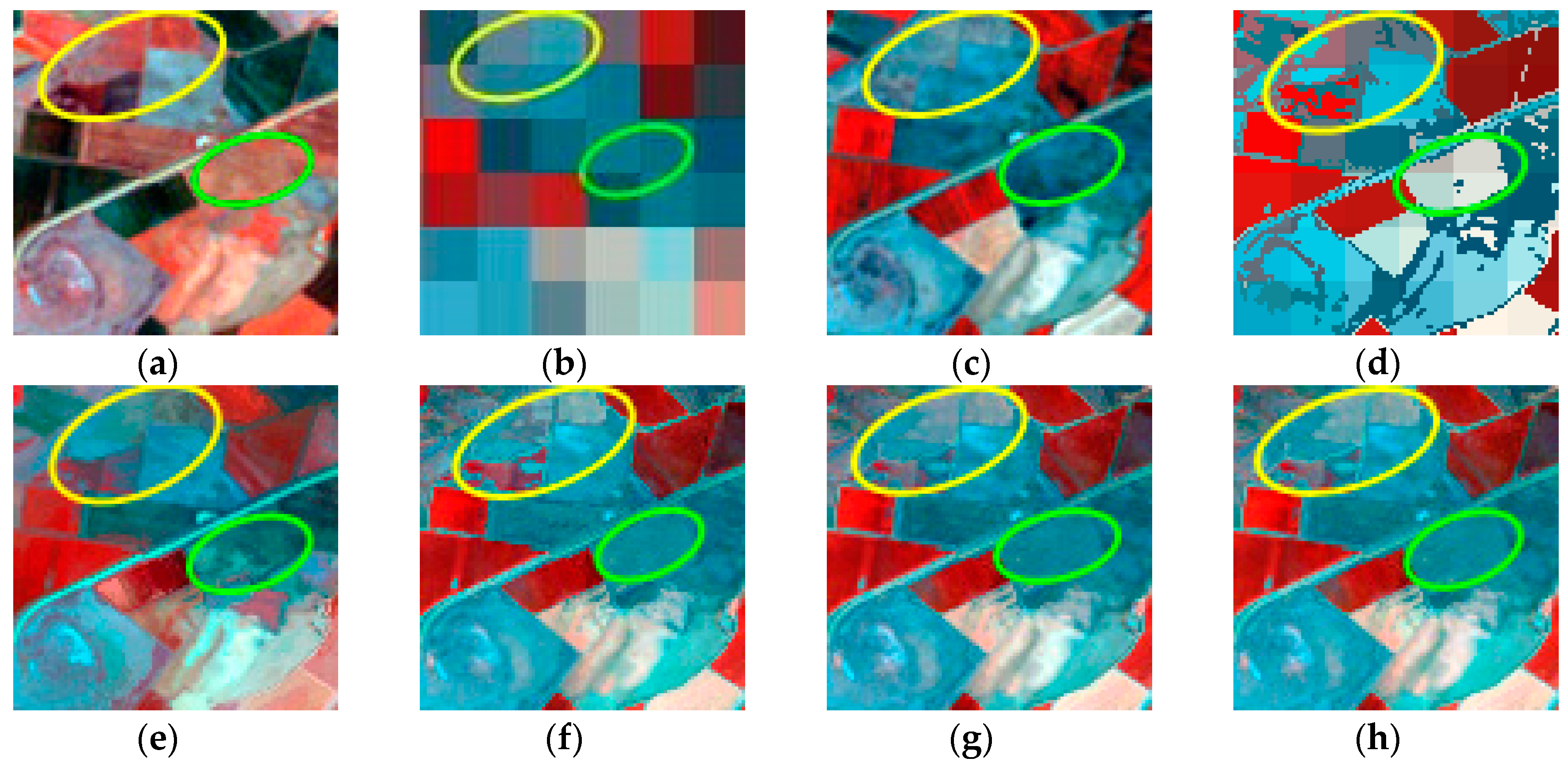
Figure 5 shows the results of the fusion predicted by the five methods. The rows from left to right successively show the two original Landsat images (see Figure 5a,b) and the UBDF, FIT-FC, FSDAF, SFSDAF, and adaptive-SFSDAF images (see Figure 5c–g), respectively. Figure 6 shows the magnified area in the yellow box in Figure 5b. It can be seen that all the fusion methods can reasonably predict the Landsat image at T2. However, the methods still have apparent differences when focusing on the spatial details of the magnified area. Particularly, it can be seen that in the yellow ellipses, the SFSDAF and adaptive-SFSDAF images are the most similar to the real Landsat image at T2, but both the FSDAF and FIT-FC images show some small crop parcels with dissimilar changes in color. UBDF has the worst performance. Generally, FSDAF and SFSDAF are better than UBDF, which can be further confirmed by the green ellipses where UBDF exhibits an incorrect white area (see Figure 6d). In addition, we can see that although adaptive-SFSDAF only performed abundance unmixing on selected pixels based on the guided mask map, there is almost no difference between SFSDAF and adaptive-SFSDAF in both the overall and detailed images.
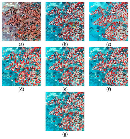
Figure 5.
Original Landsat images on December 25, 2001 (a) and January 12, 2002 (b), and the images predicted by Unmixing-Based Data Fusion (UBDF) (c), FIT-FC (d), FSDAF (e), SFSDAF (f) and adaptive-SFSDAF (g).
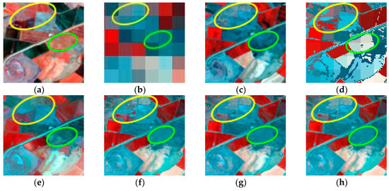
Figure 6.
Magnified images in the yellow box shown in Figure 5b: original Landsat image on 25 December 2001 (a) original MODIS-like and Landsat images on 12 January 2002 (b,c), and the images predicted by UBDF (d), FIT-FC (e), FSDAF (f), SFSDAF (g) and adaptive-SFSDAF (h).
The quantitative results are shown in Table 1. The table shows the quantitative evaluation of the original images at T1 and the fusion images from the five methods, with the real image at T2 for reference. Compared with those of SFSDAF, the indices of adaptive-SFSDAF are slightly degraded but still better than those of FSDAF. For example, band 4 has the highest temporal variation among all 6 bands (RMSE > 0.1); for adaptive-SFSDAF, the RMSE is 0.0355, with a decrease of 0.0005 compared to that of FSDAF and an increase of 0.0001 compared to that of SFSDAF. In terms of CC and SSIM of band 4, adaptive-SFSDAF has a value of 0.8427 and 0.7544, respectively, with gains of 0.0048 and 0.0056 over those of FSDAF, and with a decrease of 0.0015 and 0.0017 compared to those of SFSDAF.

Table 1.
Accuracy Assessment of the Five Fusion Methods at the Coleambally Site in Figure 3. Bold data indicate the most accurate method.
4.2. Test Using the Gwydir Dataset with Land Cover Type Change
Figure 7 presents the results of the fusion predicted by the five methods. Figure 7a,b show the two original Landsat images, while Figure 7c-g show the UBDF, FIT-FC, FSDAF, SFSDAF, and adaptive-SFSDAF images, respectively. Figure 8 shows the magnified area in the yellow box in Figure 7b. It is obvious that UBDF is the worst among the five methods, as it is not fine enough to describe flooding area at various scales (see Figure 7c, with an incorrect predicted flooding area, and Figure 8d, with blocky boundaries in detail). This is because UBDF is a local window-based unmixing method and is not suitable for landscapes with land cover type change. FIT-FC and FSDAF exhibit better prediction for the flooding areas but still has obvious dissimilar patches in the green ellipse. The SFSDAF and adaptive-SFSDAF images are the most similar to the real Landsat image. According to the visual comparison, adaptive-SFSDAF and SFSDAF are generally similar both overall and in detail.
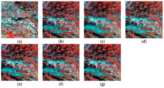
Figure 7.
Original Landsat images on November 26, 2004 (a), and December 12, 2004 (b), and the images predicted by UBDF(c), FIT-FC(d), FSDAF(e), SFSDAF(f), and adaptive-SFSDAF(g).
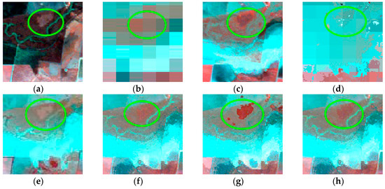
Figure 8.
Magnified images in the yellow box shown in Figure 7b: original Landsat image on 26 November 2004 (a), original MODIS-like and Landsat images on 12 December 2004 (b,c), and the images predicted by UBDF(d), FIT-FC(e), FSDAF(f), SFSDAF(g), and adaptive-SFSDAF(h).
Table 2 shows the quantitative comparison results of the five methods. It appears that UBDF has the worst performance among all the methods, which is consistent with the results reported in [20]. For all the bands, SFSDAF generated lower RMSE and MAD and higher CC, SSIM and PSNR values compared with those of FSDAF. Adaptive-SFSDAF is generally consistent with SFSDAF in terms of RMSE and MAD, but for band 4, band 5, and band 7, it predicted a slightly higher CC (band 4, 0.8971 vs. 0.895; band 5, 0.8278 vs. 0.8273; band 7, 0.8238 vs. 0.8212) and SSIM (band 4, 0.8119 vs. 0.8043; band5, 0.6391 vs. 0.6347; band 7, 0.723 vs. 0.7198) compared with those of SFSDAF. The 4th, 5th, and 7th bands have the largest temporal change among all the bands, suggesting that adaptive-SFSDAF has advantages in maintaining structural similarity for images with large temporal change.

Table 2.
Accuracy assessment of the five fusion methods at the Gwydir site in Figure 4. Bold data indicate the most accurate method.
4.3. Comparison of Computation Times
The computation times of different spatiotemporal fusion algorithms are shown in Table 3. The computer configuration for the experiments was an Intel(R) Core (TM) i7-8750H processor (2.20 Ghz) with 8 GB RAM. In our study, UBDF, SFSDAF, and adaptive-SFSDAF were implemented in MATLAB R2019a, and FIT-FC and FSDAF were implemented in ENVI5.1/IDL8.3. In order to make an accurate and fair comparison, the computation time of MATLAB platform does not include the step of reading input data or writing output data and only concerns the processing steps. The number of classes in all methods is 4. As listed in Table 3, adaptive-SFSDAF and FIT-FC are the fastest among all the models, indicating that they are both suitable for large area applications. It can be seen that in the first example, the computation time of FIT-FC and adaptive-SFSDAF was comparable; however, in the second example with larger image size, adaptive-SFSDAF was slightly faster than FIT-FC. This is mainly because the adaptive selection strategy of adaptive-SFSDAF effectively eliminates a lot of unnecessary local unmixing calculations, while FIT-FC still needs to perform local regression and spatial filter calculations pixel by pixel. It is worth mentioning that although SFSDAF has more processing steps than FSDAF, its computing efficiency is still very high because it used bicubic interpolation method instead of thin plate spline (TPS) interpolation method. UBDF is less efficient than others due to lots of local-based unmixing calculations.

Table 3.
Comparison of the computation time of different spatiotemporal fusion algorithms (unit: seconds).
The adaptive-SFSDAF proposed in this paper is an improved version of SFSDAF with greater calculation efficiency. Therefore, the focus was the comparison of the computation times between SFSDAF and adaptive-SFSDAF. As shown in Table 3, the total computation time of adaptive-SFSDAF is significantly reduced compared to that of SFSDAF. Adaptive-SFSDAF required approximately 57 s less than SFSDAF in the first example and approximately 69 s less than SFSDAF in the second example. The middle column in each example also shows the time spent solving class abundances by spectral unmixing, and the third column gives the corresponding number of unmixed pixels. Since the computation time of SFSDAF is nearly proportional to the number of coarse-resolution pixels [39], the maximum possible reduction in the number of unmixed pixels while retaining fusion performance can greatly improve the computational efficiency of SFSDAF. It is demonstrated in Table 3 that the total number of unmixed pixels of adaptive-SFSDAF in example 1 is 19.56% of that of SFSDAF, and the total number of unmixed pixels in example 2 is 22.95% of that of SFSDAF. Therefore, the time used for spectral unmixing can be reduced to approximately 20% of that of SFSDAF by adaptive-SFSDAF. For example, in experiment 1, SFSDAF required 73.3 s, whereas adaptive-SFSDAF required 14.2 s. The results in experiment 2 also support the results from experiment 1 (89.4 s for SFSDAF vs. 20.4 s for adaptive-SFSDAF).
5. Discussion
For the spatiotemporal image fusion methods used in remote sensing, spatial heterogeneity and land cover type change are two factors that greatly affect performance [11,39], To improve the processing speed of SFSDAF, adaptive-SFSDAF selectively uses class abundance change information by a guided mask map in the estimation of the temporal prediction image. Compared with SFSDAF, adaptive-SFSDAF exhibits different performance for the two typical experimental landscapes. Concrete theoretical analysis and results are described next.
5.1. Comparison of Adaptive-SFSDAF and SFSDAF for Spatially Heterogeneous Landscapes
The Coleambally dataset is for a typical spatially heterogeneous landscape. From the original two Landsat images, it can be seen that there are many small patches of fragmented crops in the scene, which have irregular shapes and a complex spatial distribution. Due to crop phenology, the reflectance values changed significantly. The difficulty of spatiotemporal image fusion for highly heterogeneous landscapes lies in the large number of mixed pixels. SFSDAF estimates both the endmember change and subpixel class fraction change when performing temporal prediction. The endmember change is derived for the entire image, while the subpixel class fraction change is estimated for each pixel; this derivation improves the inaccurate estimation of local changes in mixed pixels of heterogeneous regions. Therefore, the performance of SFSDAF is better than that of FSDAF. Adaptive-SFSDAF uses selective class abundance change information based on the guided mask map, which can be seen as a soft transition from FSDAF to SFSDAF, and its performance is generally intermediate.
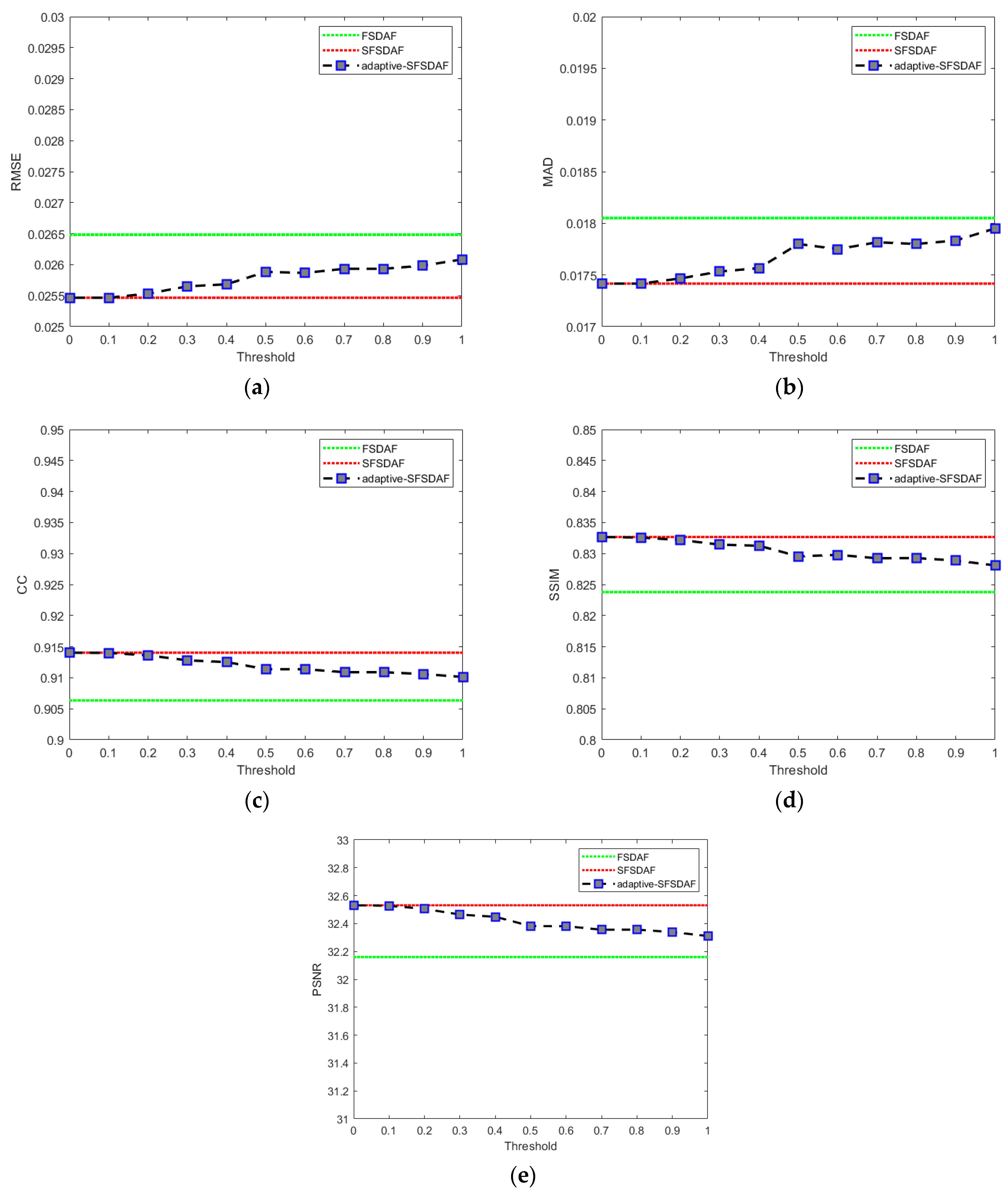
Figure 9 plots the adaptive-SFSDAF accuracy indices versus the mask threshold for the Coleambally site. The green and red lines represent FSDAF and SFSDAF, respectively. The black line between them represents adaptive-SFSDAF, which is consistent with our analysis. Furthermore, it can be seen that the curves are smoother when the mask threshold is farther away from 0.5; this indicates that, in these intervals, the performance of the fusion method does not increase as the number of unmixed pixels increases. As a result, using more pixels for unmixing did not necessarily produce better results. In general, with a decrease in the mask generation threshold, the performance of adaptive-SFSDAF will become closer to SFSDAF.
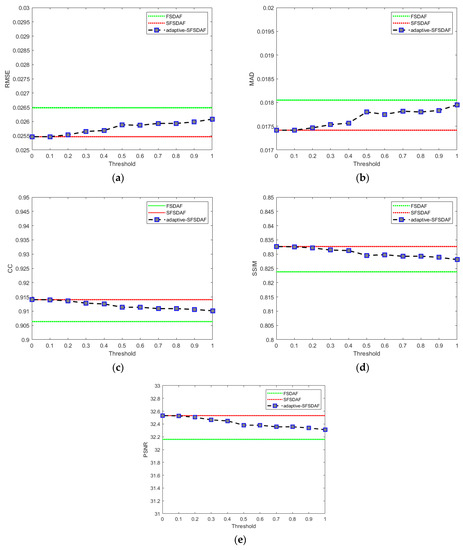
Figure 9.
Adaptive-SFSDAF accuracy indices versus the mask threshold for the Coleambally site: (a) RMSE, (b) MAD, (c) CC, (d) SSIM, and (e) PSNR. All results are the mean of total six bands.
5.2. Comparison of Adaptive-SFSDAF and SFSDAF for Landscapes with Land Cover Type Change
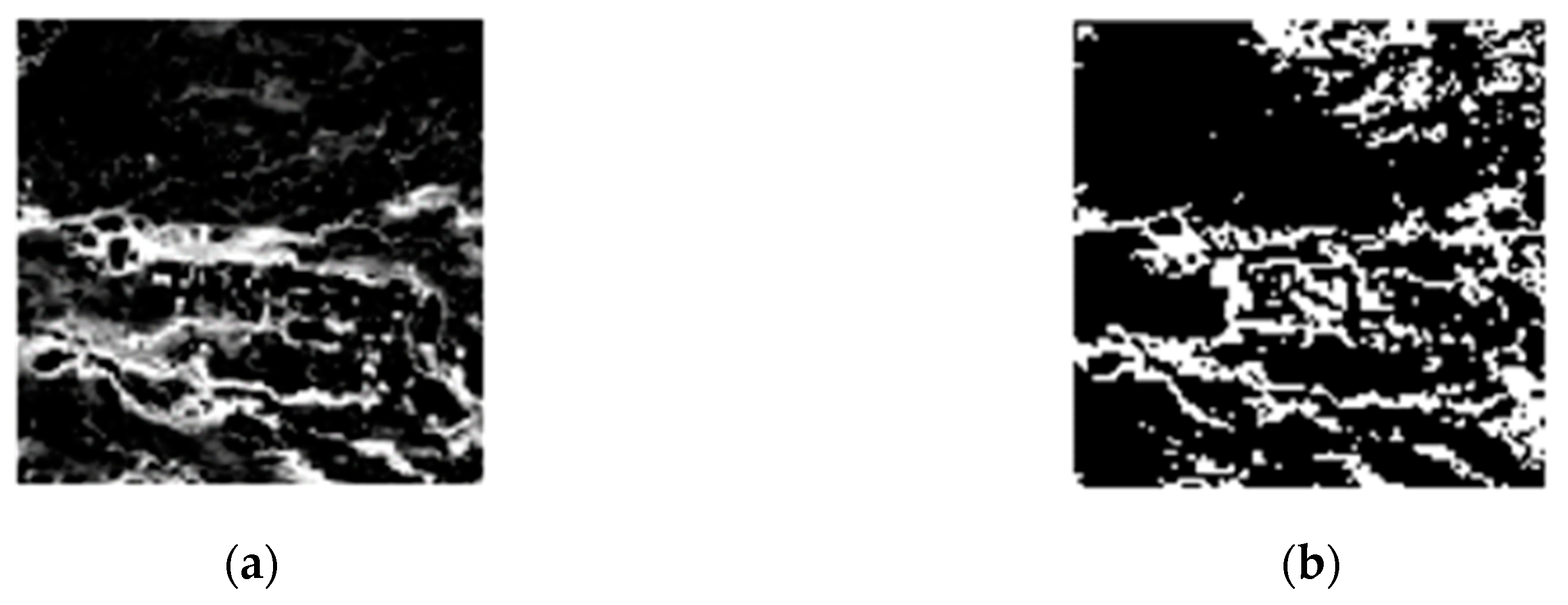
The Gwydir site is a typical landscape with land cover type change. The sudden flood event caused abrupt land cover type change between the input and prediction dates. SFSDAF incorporated the change in class abundance in each fine pixel and improved the performance compared to that of FSDAF by accurately estimating the water-inundated area. However, the inundated area only occupies a small part of the whole area and, hence, most ground cover has no abrupt land cover changes. More precisely, most pixels still exhibit global endmember changes over time. Therefore, it is not necessary to unmix all pixels one by one, which incurs a large computational burden for the fusion method. For this study area, the water abundance map at prediction time (T2) is provided in Figure 10a, and the guided mask map generated by adaptive-SFSDAF is shown in Figure 10b. We can see that the guided mask map successfully detects and covers the inundated area, indicating where land cover type change occurs. These detected outliers are very difficult to estimate and primarily affect the performance of spatiotemporal fusion methods. Adaptive-SFSDAF can adaptively detect and unmix these outliers in the image and achieve outstanding performance in balancing the computational efficiency and accuracy of the fusion results when compared to those of SFSDAF.

Figure 10.
Guided mask map for the Gwydir site: (a) the water abundance map at prediction time (T2) and (b) guided mask map.
From a methods point of view, it is known that, in order to estimate the abundance information at T2, a relatively long computation chain is used in which each step has some assumptions regarding estimation; thus, errors generated by the entire computation chain cannot be ignored. Unlike the Coleambally landscape, Gwydir has a relatively large gradually changing area, except for the abruptly flooded area. This indicates that a relatively large area contains unchanged-type pixels with approximately invariant class abundance. Using global predictions in these areas not only avoids unnecessary calculations, but also can reduce error in the long computation chain. Although a small number of pixels in the whole area are unmixed by adaptive-SFSDAF, the overall prediction error (RMSE and MAD values) does not decrease, and since the fine image at T1 provides the only true structure of the overall image, the CC and SSIM values are slightly improved in the last three spectral bands with the largest temporal change.
6. Conclusions
Spatiotemporal image fusion methods in remote sensing establish the super-resolution problem in three dimensions: time, space, and spectrum. These methods also cover the numerous advanced technologies of remote sensing intelligent processing such as weighting functions, unmixing, regression, machine learning, and so on. The development of fusion methods effectively improved the utilization of the large amount of multi-modal remote sensing data and promoted the wide application of satellite remote sensing to human activity and disaster monitoring, among other applications. Adaptive-SFSDAF is based on SFSDAF, which is the best-performing method among existing spatiotemporal fusion methods with minimal input pairs presented recently. By adaptively selecting class abundance change information for temporal estimation, adaptive-SFSDAF significantly reduced the number of unmixed pixels while retaining outstanding fusion performance. Two groups of challenging landscapes with high heterogeneity and abrupt land cover type change are selected to analyze the performance of adaptive-SFSDAF. The experimental results showed that adaptive-SFSDAF could effectively reduce the computation of unmixing processing with very little loss of fusion performance. More specifically, the following conclusions were drawn for each specific type of site: (1) for landscapes with high heterogeneity, due to a large number of mixed pixels contained in the image, the quality index performance of adaptive-SFSDAF falls between those of FSDAF and SFSDAF. However, visual comparisons of adaptive-SFSDAF and SFSDAF show no substantial differences; (2) for landscapes with land cover type change, adaptive-SFSDAF did not show degraded fusion performance. On the contrary, it had slightly higher performance in terms of retaining the image structure. Therefore, unmixing all abundance changes in the scene would not ensure better performance for fusion methods.
It is worth emphasizing that since adaptive-SFSDAF is built on SFSDAF, it is also not suitable for predicting products (such as the vegetation index [41], surface temperature [42], etc.) with only one band. In addition, although SFSDAF improved performance by incorporating class abundance changes in temporal estimates, it is much more sensitive to the registration error of the coarse-fine image pair since all class abundance change estimation occurs inside a single coarse-fine pixel pair. Adaptive-SFSDAF reduced the number of unmixed pixels and, hence, reduced this sensitivity to some extent. However, how to further improve the robustness of the fusion method to registration errors is still worthy of further discussion.
Author Contributions
Conceptualization, S.H. and W.S.; methodology, S.H. and B.G.; writing—original draft preparation, S.H., W.S., C.L. and X.L.; writing—review and editing, S.H., C.L., X.L., Y.S. and B.G.; supervision, Y.S. and J.Z. All authors have read and agreed to the published version of the manuscript.
Funding
This research was funded by the National Natural Science Foundation of China (No. 61571346; No. 61801377).
Acknowledgments
The authors gratefully acknowledge Xiaodong Li at the Institute of Geodesy and Geophysics of the Chinese Academy of Sciences for many helpful discussions. They thank Xiaolin Zhu and team at the Hong Kong Polytechnic University for providing the source code and also for their assistance in the use of the software. They thank Jin Chen for making the fusion software publicly available and Xuehong Chen for his assistance in the use of the software. They would also like to thank Maolin Liu at Peking University, Feng Gao at U.S. Department of Agriculture, and Frank Thonfeld at the University of Würzburg for their valuable helps. Finally, they wish to thank the anonymous reviewers and the editors for their constructive comments, which have improved the content of this paper.
Conflicts of Interest
The authors declare no conflict of interest.
Abbreviations
| K | denotes the number of classes |
| N | denotes the number of selected coarse pixels |
| l | denotes the number of bands |
| t1 | denotes the observation date T1 |
| t2 | denotes the observation date T2 |
| ξ | denotes the mask generation threshold |
| n | denotes the total number of similar pixels |
| C(xi,yi,t1) | denotes the ith coarse pixel value at T1 |
| C(xi,yi,t2) | denotes the ith coarse pixel value at T2 |
| ∆F (c) | denotes the cth endmember change information from T1 to T2 |
| ∆FT | denotes the estimated temporal change information from T1 to T2 |
| ∆T(xi,yi,b) | denotes the ith difference value between C(xi,yi,t2) and C(xi,yi,t1) in band b |
| denotes the ith difference vector between C(xi,yi,t2) and C(xi,yi,t1) | |
| denotes the ith estimated temporal change due to endmember change from T1 to T2 | |
| λ(xi,yi) | denotes the ith normalized measure index, which ranges from 0 to 1 |
| mask(xi,yi) | denotes the ith binary mask value |
References
- Gao, F.; Masek, J.; Schwaller, M.; Hall, F. On the blending of the Landsat and MODIS surface reflectance: Predicting daily Landsat surface reflectance. IEEE Trans. Geosci. Remote Sens. 2006, 44, 2207–2218. [Google Scholar] [CrossRef]
- Mitchell, A.L.; Rosenqvist, A.; Mora, B. Current remote sensing approaches to monitoring forest degradation in support of countries measurement, reporting and verification (MRV) systems for REDD+. Carbon Balance Manag. 2017, 12, 9. [Google Scholar] [CrossRef] [PubMed]
- Hilker, T.; Wulder, M.A.; Coops, N.C.; Linke, J.; McDermid, G.; Masek, J.G.; Gao, F.; White, J.C. A new data fusion model for high spatial- and temporal-resolution mapping of forest disturbance based on Landsat and MODIS. Remote Sens. Environ. 2009, 113, 1613–1627. [Google Scholar] [CrossRef]
- Rogan, J.; Chen, D. Remote sensing technology for mapping and monitoring land-cover and land-use change. Prog. Plan. 2004, 61, 301–325. [Google Scholar] [CrossRef]
- Zhang, J.; Zhou, C.; Xu, K.; Masataka, W. Flood disaster monitoring and evaluation in china. Glob. Environ. Chang. Part B Environ. Hazards 2002, 4, 33–43. [Google Scholar] [CrossRef]
- Joyce, K.E.; Belliss, S.E.; Samsonov, S.V.; McNeill, S.J.; Glassey, P.J. A review of the status of satellite remote sensing and image processing techniques for mapping natural hazards and disasters. Prog. Phys. Geogr. 2009, 33, 183–207. [Google Scholar] [CrossRef]
- Malingreau, J.P. Remote sensing and disaster monitoring—A review of applications in Indonesia. In Proceedings of the 18th International Symposium on Remote Sensing of Environment, Paris, France, 1–5 October 1984; pp. 283–297. [Google Scholar]
- Belgiu, M.; Stein, A. Spatiotemporal image fusion in remote sensing. Remote Sens. 2019, 11, 818. [Google Scholar] [CrossRef]
- Wang, Q.; Atkinson, P.M. Spatio-temporal fusion for daily Sentinel-2 images. Remote Sens. Environ. 2018, 204, 31–42. [Google Scholar] [CrossRef]
- Chen, B.; Huang, B.; Xu, B. Comparison of spatiotemporal fusion models: A review. Remote Sens. 2015, 7, 1798–1835. [Google Scholar] [CrossRef]
- Zhu, X.; Helmer, E.H.; Gao, F.; Liu, D.; Chen, J.; Lefsky, M.A. A flexible spatiotemporal method for fusing satellite images with different resolutions. Remote Sens. Environ. 2016, 172, 165–177. [Google Scholar] [CrossRef]
- Zhong, D.; Zhou, F. A Prediction Smooth Method for Blending Landsat and Moderate Resolution Imagine Spectroradiometer Images. Remote Sens. 2018, 10, 1371. [Google Scholar] [CrossRef]
- Zhong, D.; Zhou, F. Improvement of clustering methods for modelling abrupt land surface changes in satellite image fusions. Remote Sens. 2019, 11, 1759. [Google Scholar] [CrossRef]
- Huang, B.; Zhang, H. Spatio-temporal reflectance fusion via unmixing: Accounting for both phenological and land-cover changes. Int. J. Remote Sens. 2014, 35, 6213–6233. [Google Scholar] [CrossRef]
- Zhao, Y.; Huang, B.; Song, H. A robust adaptive spatial and temporal image fusion model for complex land surface changes. Remote Sens. Environ. 2018, 208, 42–62. [Google Scholar] [CrossRef]
- Wang, J.; Huang, B. A rigorously-weighted spatiotemporal fusion model with uncertainty analysis. Remote Sens. 2017, 9, 990. [Google Scholar] [CrossRef]
- Wu, B.; Huang, B.; Cao, K.; Zhuo, G. Improving spatiotemporal reflectance fusion using image inpainting and steering kernel regression techniques. Int. J. Remote Sens. 2016, 38, 706–727. [Google Scholar] [CrossRef]
- Kwan, C.; Budavari, B.; Gao, F.; Zhu, X. A hybrid color mapping approach to fusing MODIS and Landsat images for forward prediction. Remote Sens. 2018, 10, 520. [Google Scholar] [CrossRef]
- Kwan, C.; Zhu, X.; Gao, F.; Chou, B.; Perez, D.; Li, J.; Shen, Y.; Koperski, K.; Marchisio, G. Assessment of spatiotemporal fusion algorithms for planet and worldview images. Sensors 2018, 18, 1051. [Google Scholar] [CrossRef]
- Liu, M.; Ke, Y.; Yin, Q.; Chen, X.; Im, J. Comparison of five spatio-temporal satellite image fusion models over landscapes with various spatial heterogeneity and temporal variation. Remote Sens. 2019, 11, 2612. [Google Scholar] [CrossRef]
- Zhu, X.; Chen, J.; Gao, F.; Chen, X.; Masek, J.G. An enhanced spatial and temporal adaptive reflectance fusion model for complex heterogeneous regions. Remote Sens. Environ. 2010, 114, 2610–2623. [Google Scholar] [CrossRef]
- Chen, B.; Chen, L.; Huang, B.; Michishita, R.; Xu, B. Dynamic monitoring of the Poyang Lake wetland by integrating Landsat and MODIS observations. ISPRS J. Photogramm. Remote Sens. 2018, 139, 75–87. [Google Scholar] [CrossRef]
- Emelyanova, I.V.; McVicar, T.R.; Van Niel, T.G.; Li, L.T.; van Dijk, A.I. Assessing the accuracy of blending Landsat–MODIS surface reflectances in two landscapes with contrasting spatial and temporal dynamics: A framework for algorithm selection. Remote Sens. Environ. 2013, 133, 193–209. [Google Scholar] [CrossRef]
- Bioucas-Dias, J.M.; Plaza, A.; Dobigeon, N.; Parente, M.; Du, Q.; Member, S.; Chanussot, J. Hyperspectral unmixing overview: Geometrical, statistical, and sparse regression-based approaches. IEEE J. Sel. Top. Appl. Earth Obs. Remote Sens. 2012, 5, 354–379. [Google Scholar] [CrossRef]
- Amorós-López, J.; Gómez-Chova, L.; Alonso, L.; Guanter, L.; Zurita-Milla, R.; Moreno, J.; Camps-Valls, G. Multitemporal fusion of Landsat/TM and ENVISAT/MERIS for crop monitoring. Int. J. Appl. Earth Obs. Geoinf. 2013, 23, 132–141. [Google Scholar] [CrossRef]
- Zhukov, B.; Oertel, D.; Lanzl, F.; Reinhäckel, G. Unmixing-based multisensory multiresolution image fusion. IEEE Trans. Geosci. Remote Sens. 1999, 37, 1212–1226. [Google Scholar] [CrossRef]
- Zurita-Milla, R.; Clevers, J.G.; Schaepman, M.E. Unmixing-based Landsat TM and MERIS FR data fusion. IEEE Geosci. Remote Sens. Lett. 2008, 5, 453–457. [Google Scholar] [CrossRef]
- Zurita-Milla, R.; Kaiser, G.; Clevers, J.; Schneider, W.; Schaepman, M. Downscaling time series of MERIS full resolution data to monitor vegetation seasonal dynamics. Remote Sens. Environ. 2009, 113, 1874–1885. [Google Scholar] [CrossRef]
- Gevaert, C.M.; García-Haro, F.J. A comparison of STARFM and an unmixing-based algorithm for Landsat and MODIS data fusion. Remote Sens. Environ. 2015, 156, 34–44. [Google Scholar] [CrossRef]
- Ma, J.; Zhang, W.; Andrea, M.; Gao, L.; Zhang, B. An Improved Spatial and Temporal Reflectance Unmixing Model to Synthesize Time Series of Landsat-Like Images. Remote Sens. 2018, 10, 1388. [Google Scholar] [CrossRef]
- Xue, J.; Leung, Y.; Fung, T. An Unmixing-Based Bayesian Model for Spatio-Temporal Satellite Image Fusion in Heterogeneous Landscapes. Remote Sens. 2019, 11, 324. [Google Scholar] [CrossRef]
- Xue, J.; Leung, Y.; Fung, T. A bayesian data fusion approach to spatio-temporal fusion of remotely sensedimages. Remote Sens. 2017, 9, 1310. [Google Scholar] [CrossRef]
- Huang, B.; Song, H. Spatiotemporal reflectance fusion via sparse representation. IEEE Trans. Geosci. Remote Sens. 2012, 50, 3707–3716. [Google Scholar] [CrossRef]
- Song, H.; Huang, B. Spatiotemporal satellite image fusion through one-pair image learning. IEEE Trans. Geosci. Remote Sens. 2013, 51, 1883–1896. [Google Scholar] [CrossRef]
- Liu, X.; Deng, C.; Wang, S.; Huang, G.-B.; Zhao, B.; Lauren, P. Fast and accurate spatiotemporal fusion based upon extreme learning machine. IEEE Geosci. Remote Sens. Lett. 2016, 13, 2039–2043. [Google Scholar] [CrossRef]
- Liu, X.; Deng, C.; Chanussot, J.; Hong, D.; Zhao, B. StfNet: A Two-Stream Convolutional Neural Network for Spatiotemporal Image Fusion. IEEE Trans. Geosci. Remote Sens. 2019, 57, 6552–6564. [Google Scholar] [CrossRef]
- Tan, Z.; Yue, P.; Di, L.; Tang, J.J.R.S. Deriving high spatiotemporal remote sensing images using deep convolutional network. Remote Sens. 2018, 10, 1066. [Google Scholar] [CrossRef]
- Song, H.; Liu, Q.; Wang, G.; Hang, R.; Huang, B. Spatiotemporal Satellite Image Fusion Using Deep Convolutional Neural Networks. IEEE J. Sel. Top. Appl. Earth Obs. Remote Sens. 2018, 11, 821–829. [Google Scholar] [CrossRef]
- Li, X.; Foody, G.M.; Boyd, D.S.; Ge, Y.; Zhang, Y.; Du, Y.; Ling, F. Sfsdaf: An enhanced fsdaf that incorporates sub-pixel class fraction change information for spatio-temporal image fusion. Remote Sens. Environ. 2019, 237. [Google Scholar] [CrossRef]
- Ball, G.H.; Hall, D.J. ISODATA, A Novel Method of Data Analysis and Pattern Classification; Technical Report; Stanford Research Institute: Menlo Park, CA, USA, May 1965. [Google Scholar]
- Gao, F.; Hilker, T.; Zhu, X.; Anderson, M.A.; Masek, J.; Wang, P.; Yang, Y. Fusing Landsat and MODIS data for vegetation monitoring. IEEE Geosci. Remote Sens. Mag. 2015, 3, 47–60. [Google Scholar] [CrossRef]
- Quan, J. Blending multi-spatiotemporal resolution land surface temperatures over hetero-geneous surfaces. In Proceedings of the 2017 Joint Urban Remote Sensing Event (JURSE), Dubai, UAE, 6–8 March 2017. [Google Scholar] [CrossRef]
Publisher’s Note: MDPI stays neutral with regard to jurisdictional claims in published maps and institutional affiliations. |
© 2020 by the authors. Licensee MDPI, Basel, Switzerland. This article is an open access article distributed under the terms and conditions of the Creative Commons Attribution (CC BY) license (http://creativecommons.org/licenses/by/4.0/).

