Article

Surface Motion Prediction and Mapping for Road Infrastructures Management by PS-InSAR Measurements and Machine Learning Algorithms

1
Department of Civil and Industrial Engineering, Engineering School of the University of Pisa, Largo Lucio Lazzarino 1, 56126 Pisa, Italy
2
Institute of Geodesy and Photogrammetry, Technische Universität Braunschweig, Bienroder Weg 81, 38106 Braunschweig, Germany
*
Author to whom correspondence should be addressed.
Remote Sens. 2020, 12(23), 3976; https://doi.org/10.3390/rs12233976
Submission received: 28 September 2020 / Revised: 19 November 2020 / Accepted: 3 December 2020 / Published: 4 December 2020

Abstract

:
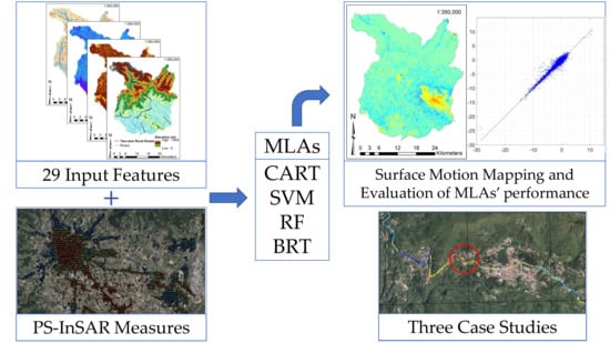
This paper introduces a methodology for predicting and mapping surface motion beneath road pavement structures caused by environmental factors. Persistent Scatterer Interferometric Synthetic Aperture Radar (PS-InSAR) measurements, geospatial analyses, and Machine Learning Algorithms (MLAs) are employed for achieving the purpose. Two single learners, i.e., Regression Tree (RT) and Support Vector Machine (SVM), and two ensemble learners, i.e., Boosted Regression Trees (BRT) and Random Forest (RF) are utilized for estimating the surface motion ratio in terms of mm/year over the Province of Pistoia (Tuscany Region, central Italy, 964 km2), in which strong subsidence phenomena have occurred. The interferometric process of 210 Sentinel-1 images from 2014 to 2019 allows exploiting the average displacements of 52,257 Persistent Scatterers as output targets to predict. A set of 29 environmental-related factors are preprocessed by SAGA-GIS, version 2.3.2, and ESRI ArcGIS, version 10.5, and employed as input features. Once the dataset has been prepared, three wrapper feature selection approaches (backward, forward, and bi-directional) are used for recognizing the set of most relevant features to be used in the modeling. A random splitting of the dataset in 70% and 30% is implemented to identify the training and test set. Through a Bayesian Optimization Algorithm (BOA) and a 10-Fold Cross-Validation (CV), the algorithms are trained and validated. Therefore, the Predictive Performance of MLAs is evaluated and compared by plotting the Taylor Diagram. Outcomes show that SVM and BRT are the most suitable algorithms; in the test phase, BRT has the highest Correlation Coefficient (0.96) and the lowest Root Mean Square Error (0.44 mm/year), while the SVM has the lowest difference between the standard deviation of its predictions (2.05 mm/year) and that of the reference samples (2.09 mm/year). Finally, algorithms are used for mapping surface motion over the study area. We propose three case studies on critical stretches of two-lane rural roads for evaluating the reliability of the procedure. Road authorities could consider the proposed methodology for their monitoring, management, and planning activities.

Graphical Abstract

1. Introduction

The different aspects of the daily life of most people and communities are intertwined with the roads [1]. Therefore, hazard prevention, planning, monitoring, inspection, and maintenance of roads network is critical. Non-Destructive High-Performance Techniques are essential tools for managing extended and complex road networks. By such techniques, road authorities can efficiently obtain reliable information concerning the causes of distresses (exogenous and endogenous factors) and consequences (infrastructure damages and deficiencies) of the assets they manage.
Currently, Persistent Scatterer Interferometric Synthetic Aperture Radar (PS-InSAR) technique is widely employed in infrastructure monitoring and inspection since it allows achieving reliable outcomes in the identification and prevention of infrastructural instabilities over time. However, PS-InSAR provides a point-based outcome and, therefore, infrastructures are not generally covered wholly by PS measures. Especially by using non-high-resolution satellites, there is usually no sufficient and homogeneous number of PS for assessing the condition of the assets, comprehensively. Besides, the PS-InSAR technique is not able to define the causes that produce surface motions. Considering the strengths and weaknesses of PS-InSAR for road monitoring and inspection activities, it is essential to optimize its functionality. To the best of our knowledge, little or nothing has been discussed on the use of PS-InSAR outcomes for modeling and predicting infrastructure instabilities for road infrastructure monitoring and management.
Accordingly, this research fits into the field of road maintenance using SAR-based sensors, through which we want to investigate the possibility of defining a predictive and preventive strategy. In other words, we aim to define a methodology that is able to exploit the PS-InSAR survey and allows mapping the surface movement at any point over infrastructures. Furthermore, this methodology should be able to predict instabilities even where PS are absent, and also highlight the causes of such motions, enabling road authorities to intervene before the triggering of a potentially critical phenomenon. By exploiting this strategy, road authorities should optimize the prevention, planning, monitoring, inspection, and maintenance of their network.
The primary hypothesis of the present research is that the surface motion recorded by the PS-InSAR technique can be correlated to road pavement deformations and damages. Once the Machine Learning Algorithms (MLAs) have been calibrated, through this assumption, it is possible to map surface movements and detect where road pavement structures are damaged.
In combination with SAR, the proposed methodology exploits the capability of advanced statistical modeling, such as MLAs, that can associate the most relevant conditioning factors with the target variable examined. Such target output (i.e., the dependent variable of the MLAs) is the average yearly surface motion identified by a PS-InSAR survey. In contrast, conditioning factors (i.e., the independent variables of the MLAs) are associated with exogenous events of infrastructures. Such events can alter infrastructure quality and are associated with natural phenomena, such as earthquakes, landslides, subsidence, sinkholes, and floods. Such events can be triggered by topological, geomorphological, hydrological, and social systems of the surrounding environment of infrastructures. The suggested methodology should enhance the feasibility of well-structured road maintenance plans, recognizing the most relevant interventions that infrastructures demand in advance.
This paper is an extended and updated version of Reference [2]. Specifically:
  • An extensive literature review has been conducted in all sections of the paper by adding 120 references;
  • This study proposes a prediction of surface motion rate for an extended area (from 132 km2 to 964 km2);
  • A wrapper feature selection approach has been introduced in order to reduce the computational complexity of the algorithms, improving their interpretability, reduce overfitting issues, and also increase the overall predictive performance. Our previous study did not include this preprocessing step;
  • Only PS observations have been used as target output to be modeled. Conversely, in Reference [2], we considered as output an interpolated map of PS-InSAR measures realized by the Inverse Distance Weighting process. Therefore, in this paper, we deal with real observation, avoiding the hypothesis that the measurements are correlated with each other through a predetermined distance function;
  • In this paper, we not only used Regression Tree (RT) algorithm that was used in Reference [2] but also investigated three MLAs, namely Support Vector Machine (SVM), Random Forest (RF), and Boosted Regression Trees (BRT);
  • Bayesian Optimization Algorithm (BOA) and 10-Fold Cross-Validation (CV) have been implemented to ensure that the best set of hyperparameters has been found out automatically. Therefore, we avoided to use of manual, random, or grid searches (that require user experience and a higher computational cost);
  • The Taylor Diagram and scatterplots have been computed to evaluate and compare the algorithms appropriately (in addition to R2, Root Mean Square Error (RMSE), and Mean Absolute Error (MAE));
  • Once the surface motion maps have been computed, we propose two additional case studies (i.e., two critical road sites) for evaluating the reliability of the suggested methodology.
The remainder of this paper is organized as follows: In Section 2, InSAR techniques for road monitoring are reviewed and several papers where the authors dealt with Machine Learning for modeling environmental-related issues are mentioned. In Section 3, the methodology: study area, workflow, database preparation (data collection, input/output definition, and feature selection), MLAs implementation (training, validation, test, evaluation, and comparison) are described. Afterward, in Section 4, the main findings of the research and future works are reported and discussed. Finally, the closing discussion and conclusion are presented in Section 5.

2. Related Works

2.1. InSAR Techniques and InSAR for Road Monitoring and Inspection

SAR is an active sensor mounted on both airborne and spaceborne platforms able to realize high-resolution radar images of the earth’s surface. SAR uses the microwave band in the broad radio spectrum; thus, it can provide images during day and night, and it can penetrate cloud cover and, sometimes, rain [3].
In 1974 the concept of SAR interferometry (InSAR) for earth’s surface observation had been introduced [4]. Differential InSAR (D-InSAR) technique has been developed to measure gradual surface motion between a couple of SAR image acquisitions. The core idea is to observe the difference between phase information that is correlated to the spatial changes of surface height. Therefore, D-InSAR can produce accurate digital elevation models (DEM) at a relatively low cost and detect deformation caused by various phenomena, such as earthquakes, volcanic activities, and glacier flows. D-InSAR allows monitoring large areas [5] with accuracy within centimeters to millimeters. Unfortunately, the accuracy of D-InSAR could be affected and reduced by two primary issues: temporal and geometric decorrelation and phase distortion due to atmospheric circumstances. Furthermore, since D-InSAR exploits only two SAR images, it is not capable of describing displacement patterns over time.
PS-InSAR has been promoted to overcome the drawbacks of D-InSAR. Indeed, by employing a long stack of co-registered SAR images, a PS-InSAR survey allows practitioners to visualize displacement patterns and quantify surface motion over time efficiently [6,7,8]. The PS-InSAR technique provides a point-based map outcome, in which a massive amount of Persistent (or Permanent) Scatterers (PS) is generally detected. PS are on-ground stable items for which spectral response does not change significantly during various SAR image acquisitions. Phase information backscattered from PS is used to determine the intensity and the temporal pattern of the surface motion along the Line-Of-Sight of the SAR sensor. Starting from a reference image, called the master image, each new acquisition allows adding a displacement value to each detected PS. To obtain a concise value, all recorded values are averaged, thus obtaining the average displacement over time, i.e., the average deformation velocity (or surface motion rate) of each PS. This deformation rate is generally expressed in millimeters/year.
The highest performance of PS-InSAR is provided in surveys on urbanized areas and infrastructures, where several stable PS can be found [7,9]. The technique has been used broadly for monitoring slow or relatively slow movements caused by human-related factors, such as mining activities [10,11], tunneling [12,13], and groundwater extraction [14]. Moreover, PS-InSAR can detect efficiently phenomena in which the environment plays also a key role, e.g., subsidence phenomena [15,16,17,18,19,20], landslides [21,22,23,24,25,26,27], sinkholes [20,28,29,30,31], active rock glacier movements [32,33], and displacement patterns driven by permafrost processes [34]. Nonetheless, there are some practice barriers to the use of PS-InSAR; the most significant flaw of this technique is the lack of PS in non-urbanized areas (e.g., agricultural and forested regions), where irregularities in geometry among SAR acquisitions generate phase decorrelation and cause a problematic PS identification [35].
In contrast, the ability to efficiently detect surface movements over urbanized large areas with relatively high accuracy and resolution has allowed the PS-InSAR technique to be developed in the field of Non-Destructive High-Performance civil infrastructure survey. The range of activities is broad:
  • planning, where the PS-InSAR technique is implemented for identifying areas where building new infrastructures [36];
  • prevention, where PS-InSAR is used to provide maintenance plans relying on the magnitude of the detected surface motion [37];
  • monitoring and inspection, an interferometric process is used to detect critical infrastructural damages, identifying sections in which there are substantial movements [38]. We found researches on the implementation of PS-InSAR for road infrastructures [36,37,38,39,40,41,42], rail infrastructures [29,43,44,45,46], bridges [47,48,49,50], and dams [51,52,53,54];
Furthermore, Ozden et al. [55] demonstrated by an InSAR benefit/cost analysis that SAR-based monitoring improves the effectiveness of the overall infrastructure monitoring system and reduces the total cost. Furthermore, it is worth mentioning that the effect of traffic jams on SAR images can be avoided as described in Reference [42]. The authors stated that the PS-InSAR outcomes can be used efficiently for predicting the quality of pavement, and that results are comparable with in-situ road roughness measurement.

2.2. Environmental Modeling by Machine Learning Modeling

To the best of our knowledge, there is not so much research on the prediction of surface motion ratio exploiting PS-InSAR measurement and MLAs. In addition to our previous research [2], it is worth mentioning the work of Deng et al. [56], in which the authors used a Grey–Markov model to predict subsidence ratio by exploiting PS-InSAR measures. However, such a study is different since they did not use environmental parameters for predicting subsidence detected by InSAR, and suggest a prediction of subsidence by a probabilistic approach.
Therefore, the purpose of this subsection is to identify how researchers use MLAs to map the susceptibility of areas to major natural or human-induced phenomena that cause massive economic and social losses to the community. We would like to highlight the most investigated issues, the most implemented MLAs, and the way for evaluating their modeling. Table 1 proposes a review of more than 40 recent works on environmental modeling by MLAs. It reports the reference (Ref.), the environmental-related issue investigated (Topic), the type of modeling (Task), i.e., if the MLAs have been used for classification (C) or Regression (R) purposes, the algorithms implemented (MLAs), the metrics employed for their evaluation (Performance Metrics), and if the authors made a feature selection approach in a preprocessing stage before training the MLAs.
Table 1 provides an overview depicting the following aspects:
  • Most of the studies involve the prediction of landslides, probably because they are the phenomenon that is most manifested worldwide. Some other relevant topics are flood susceptibility, gully erosion by stream power, and groundwater potential mapping. Subsidence, settlements, uplift, and, in general, surface motion prediction seems to have a lower interest from the academic community. However, the losses caused by these effects can still be enormous, and it is essential to be able to predict and mitigate their effects;
  • Most of the study involves a classification approach, i.e., the MLAs are calibrated for providing a binary output; thus, they can predict the presence or the absence of the phenomena, but nothing can be said regarding the intensity, the duration, and the direction. Conversely, Regression approaches attempt to predict a numerical output, i.e., they can provide information regarding a parameter of interest of a phenomenon (e.g., the safety factor in slope stability assessment or the settlement ratio in subsidence modeling). They suppose that a phenomenon could manifest over the entire study area;
  • An extensive set of implemented MLAs has been identified. There are numerous studies in which the algorithms are single learners (such as Classification and Regression Tree (CART) or SVM), and several ones in which ensemble learners are adopted (through aggregation techniques, such as bagging or boosting). Generally, they belong to three families: tree-based models (e.g., CART, RF, and BRT), Artificial Neural Network (ANN)-based models, and SVM-based models. Other algorithms often used are Logistic Regression (LR), Frequency Ratio (FR) (they only work for classification tasks), and Multivariate Adaptive Regression Splines (MARS). Other types of algorithms, less used, are shown in Table 1;
  • The metrics for evaluating the performance of MLAs are also manifold. The vast majority of classification-based studies present the calculation of the Area Under the Receiver Operating Characteristic (AUROC) and Accuracy. In regression-based studies, the most common parameters are the R2, RMSE, and MAE;
  • A feature selection approach before the training phase is not always implemented. Indeed, in about half of the reviewed papers, the authors declare that the set of conditioning factors is defined relying on expert judgment or their previous implementation in other papers, or simply describe the set of parameters without precise justifications. It must be said, however, that the set of conditioning factors are often the same for all the reviewed studies.
  • When a feature selection approach is implemented, the computation of the Variance Inflation Factors (VIF) has often been found. This parameter tests the multicollinearity of the factors, excluding the redundant ones. Unfortunately, VIF can only consider linear relationships between features, and in complex phenomena, this hypothesis appears strong. However, the VIF proposes a simple calculation, and the experience demonstrated by its extensive use shows that it still has a beneficial effect on modeling. Sometimes authors decide to test different subsets of features (for example, using a set with few features and a set with many of them) and compare the performance of MLAs. This technique could be useful for identifying a good subset of features excluding the less relevant ones, but if the subdivision into different datasets does not follow a specific algorithm, a satisfactory result is not guaranteed. More sophisticated feature selection methods, such as Principal Component Analysis (PCA) or Wrapper approaches, have been identified in limited research. Although they are powerful techniques, their limited use could derive from the excessive computational cost required.
Considering the above information highlighted by a bibliographic review, in this paper, we have decided to implement four MLAs: two single learners, i.e., RT and SVM, and two ensemble learners, i.e., RF (to exploit the advantages of bagging) and BRT (to exploit the potential of boosting). Considering that these models predict a numerical response, the metrics for evaluating their performance are the R2, RMSE, and the MAE. Furthermore, to highlight specific problems related to overfitting, clustering, or possible outliers, the scatterplots of the training and test phase are shown. Finally, to compare the MLAs from a graphical point of view, the Taylor Diagram is plotted. Three wrapper feature selection approaches are used, which allow, through an iterative and automatic procedure, to select a subset of the most relevant features for the modeling of the phenomenon. Wrappers should reduce the complexity of the phenomenon, reduce training times, alleviate possible overfitting issues, and possibly improve the performance of the models. The models are trained (the hyperparameters are tuned) automatically through the BOA and a 10-Fold CV process on 70% of the dataset (training set) and tested on the remaining 30% (test set).

3. Methodology

3.1. Study Area

The study area is the Province of Pistoia (Figure 1b), located in the Tuscany Region (Figure 1a), central Italy, and extends for 964 km2. Considering the strong subsidence that influences the Province, this area has become attractive for many authors aiming to analyze the magnitude of such effects and the associated causes; for example, there are studies involving Pistoia [16], the surrounding “Arno” river basin [35,102,103,104], and the Florence-Prato-Pistoia plain [17]. In Reference [17], the authors explained that movements are likely correlated to groundwater overexploitation by numerous nurseries opened since the 21st century. The high request for water is combined with soft layers compaction, resulting in a drop in the groundwater level and subsidence. Figure 1c describes the topography of the study area by its elevation (DEM) map; we can note a mountainous area in the northern part of the area, while two extensive flat areas are located in the southern part, divided by a not too pronounced mountain range. In the flat area on the right is located the city of Pistoia.
Furthermore, Figure 1c shows the river network. The network is made up of numerous rivers and streams, both in the mountainous and in the flat part, distributed evenly over the entire study area. These rivers flow mainly into the Arno River, the most important in the Tuscany region. Indeed, the flat areas of the study area are part of the so-called “Firenze-Pistoia-Prato” Arno river basin.
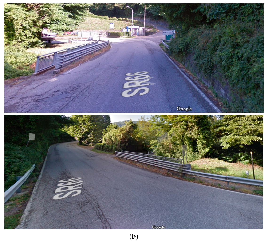
Finally, Figure 1c depicts the road network managed by the Tuscany Region Road Administration (TRRA). From an operational point of view, TRRA generally carries out monitoring and inspections of road infrastructures, plans maintenance interventions, and designs new infrastructural works. Moreover, the TRRA promotes and funds research for road safety analyses [105], planning maintenance intervention [106], mitigating road pavement noise [107,108], and using renewable materials in pavement structures [109]. In the province of Pistoia, TRRA manages three regional two-lane rural roads, called SR435, SR436, and SR66. Two-lane rural roads are single carriageway roads with one lane for each travel direction [110]. In Italy, such roads should have a lanes’ width greater than 3.75 m, paved shoulder greater than 1.50 m, a radius of curves greater than 118 m, and a maximum slope of 7%. These roads may eventually cross urban centers (such as the SR66 and SR435, which cross the city of Pistoia) for short stretches. The TRRA manages only the stretches that persist in rural areas; the suggested procedure is provided for these road sections but can be extended to the urban context.
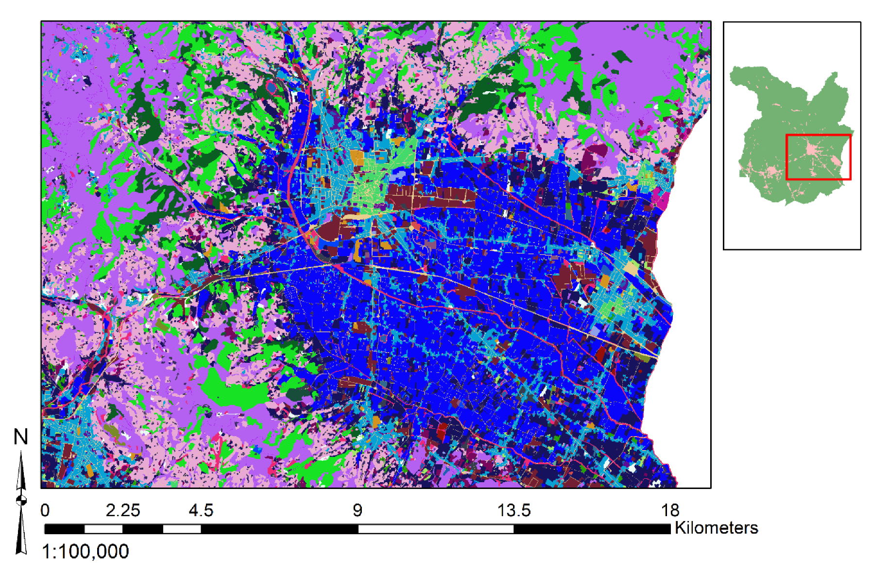
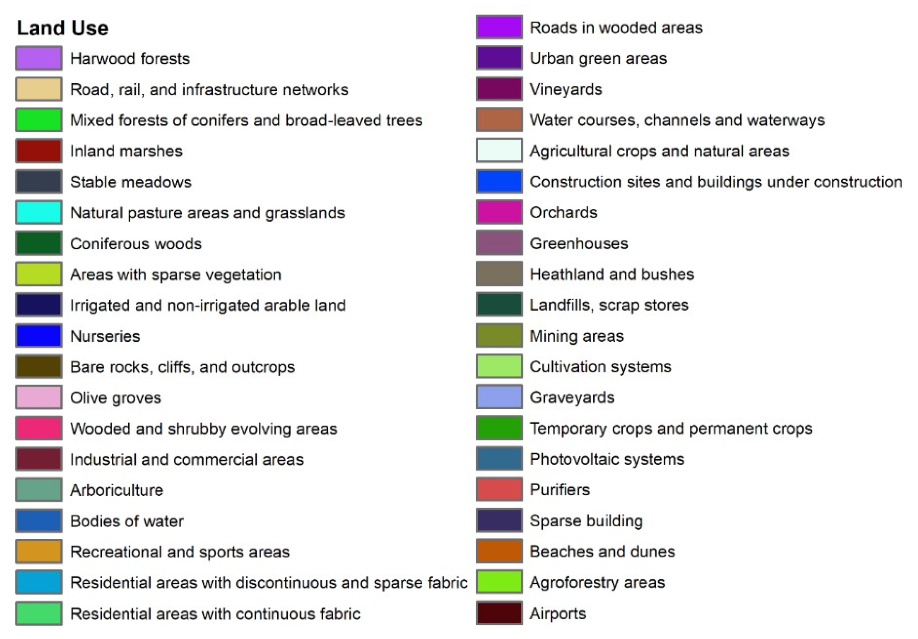
Figure 2 describes the land use map of the surrounding area of the Pistoia city center; it allows understanding the significant overexploitation of water in this area.
From Figure 2 we can note the imposing presence of nurseries ranging from the outskirts of the city to the right border of the Province. Pistoia is, in fact, one of the major European centers of nurseries. Figure A1 describes the Land Use map for the entire study area.

3.2. Workflow

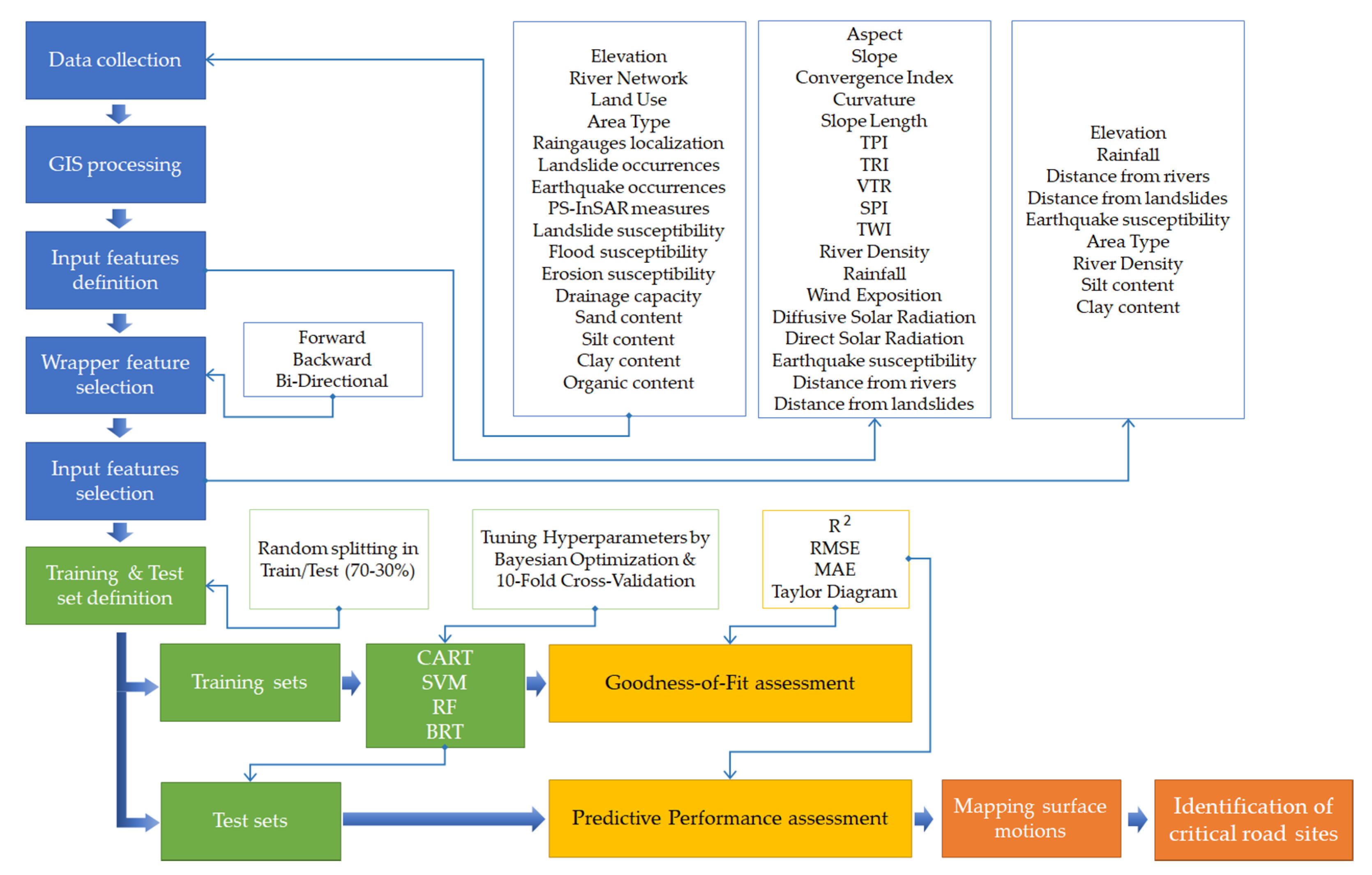
The steps of the proposed approach have been explained in Figure 3.
Firstly, data collection has been carried out. Sixteen types of information have been collected and preprocessed into a GIS platform to define the input features and the target output of the MLAs. A total of 29 input features have been computed. Subsequently, three wrapper feature selection approaches (forward, backward, and bi-directional) have been performed to identify the most relevant subset of features that can be associated with the output target. Specifically, 9 out of 29 features have been elected as input features. Once the dataset has been prepared, we randomly split it into the training (70% of the observations) and test set (30%).
Using the training set, the MLAs (RT, SVM, BRT, and RF) have been trained, validated, and evaluated by R2, RMSE, MAE, and the Scatterplots (phase of the Goodness-of-Fit assessment). The training phases of each MLA have been carried out by 30 iterations of the BOA; in each iteration, a 10-Fold CV has been implemented for evaluating the performance of the trained MLA. Therefore, the hyperparameters of the MLAs have been tuned by the BOA and CV in this phase.
Using the test set and the trained MLAs, the Predictive Performance can be evaluated by R2, RMSE, MAE, the Scatterplots, and the Taylor Diagram. In this phase, the MLAs have also been compared for identifying the most efficient and promising ones.
Once the MLAs have been trained and tested, we have employed them for making predictions and mapping the surface motion ratio over the whole study area, even in areas where there are no PS measurements.
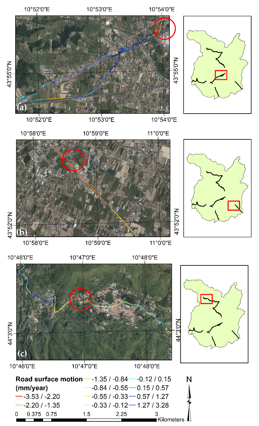
Finally, we have overlayed the road network that crosses the study area with the predicted surface motion maps; thus, it is possible to detect all the critical road sites of the network and draw up a priority road inspection list for planning a monitoring and inspection activity. For ensuring the reliability of the suggested approach, we propose three case studies of road sites predicted as critical by MLAs. The following subsections describe each of these phases.

3.3. Database Preparation

3.3.1. Data Collection

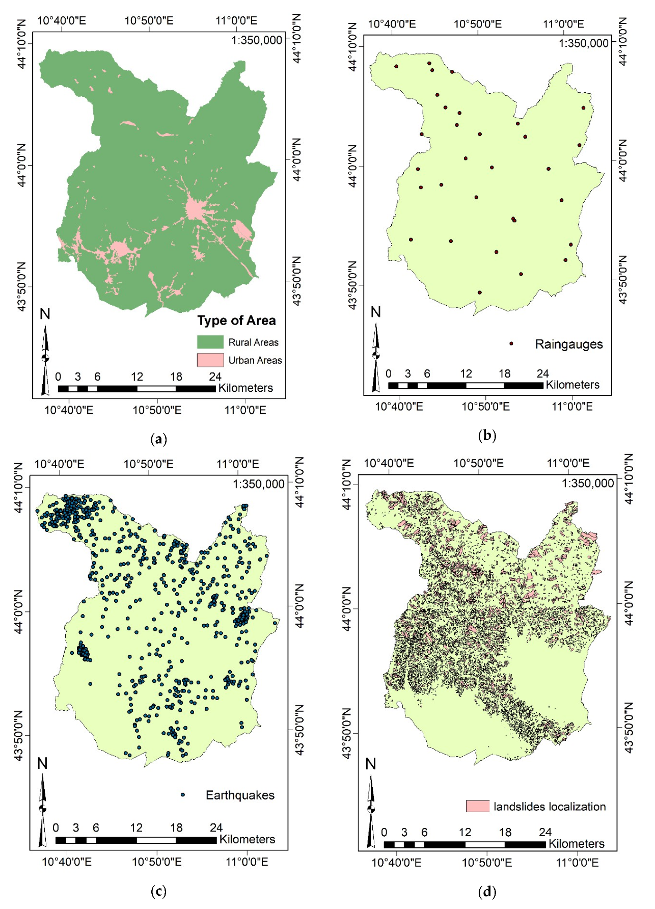
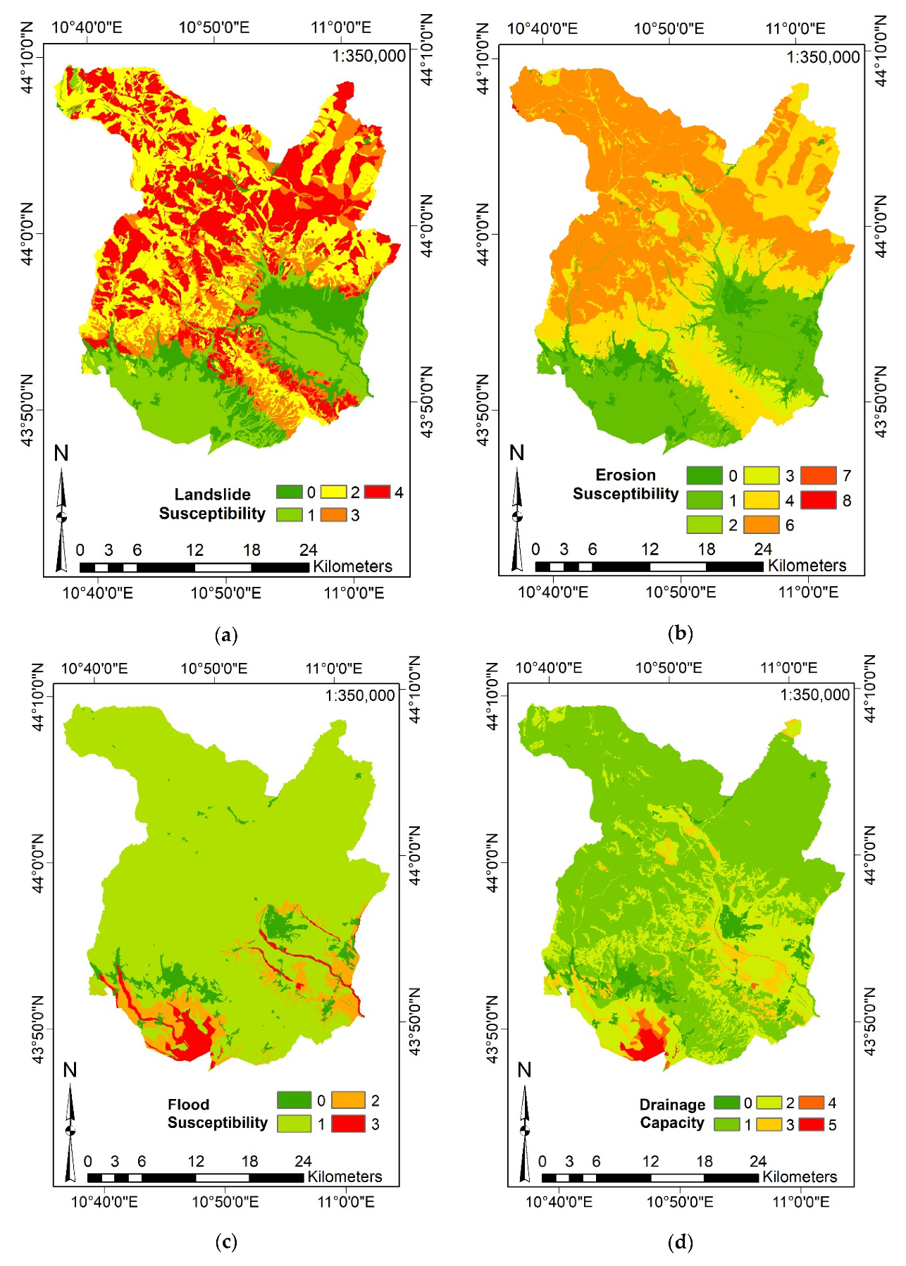
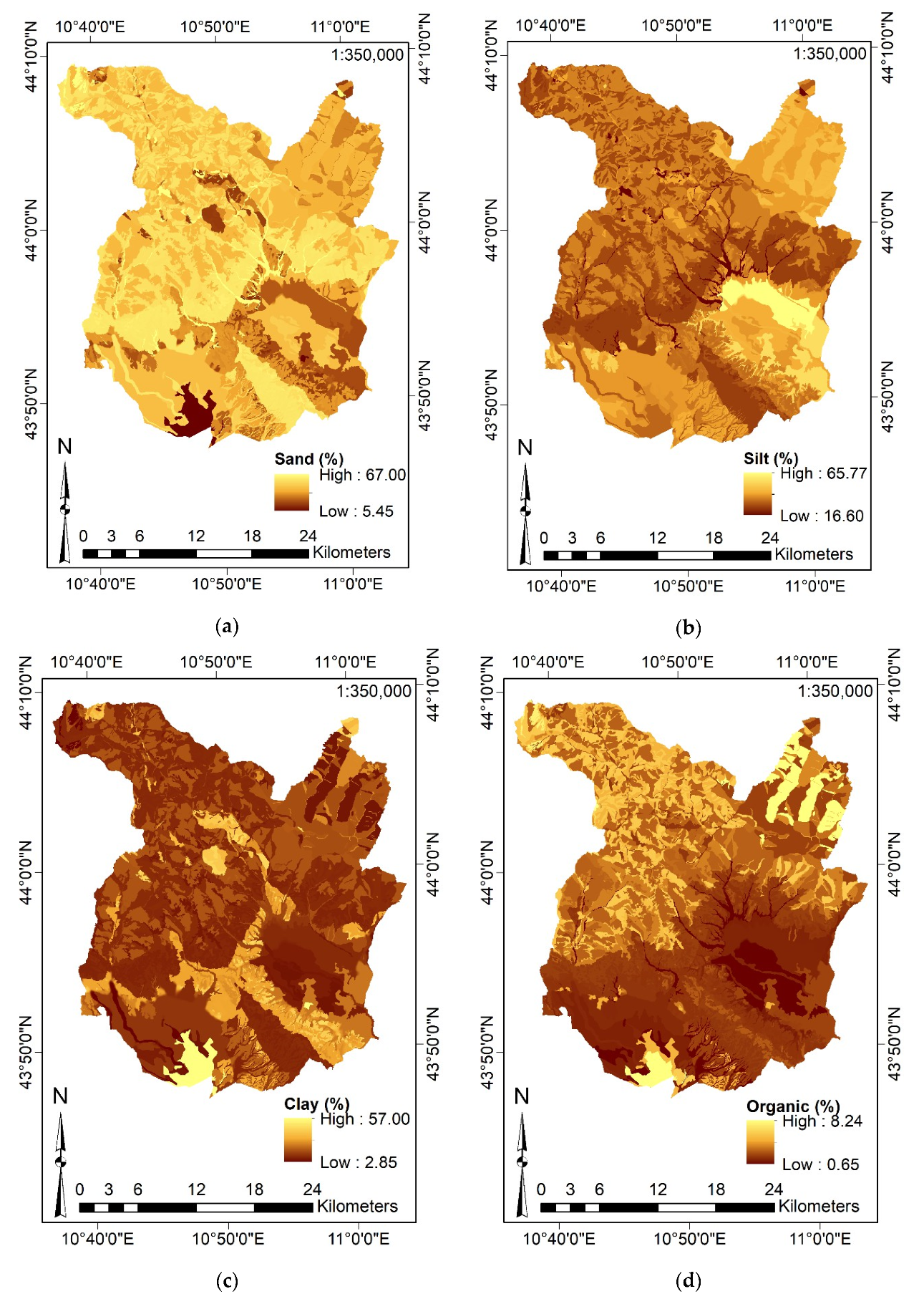
Sixteen types of information have been collected, including elevation, river network, land use, area type (i.e., localization of the urban and rural areas), localization of the rain gauges and rainfall data from 2014 to 2019, landslides (localization) and earthquakes (localization and magnitude) occurred, landslide susceptibility, flood susceptibility, erosion susceptibility, drainage capacity of the soil, and sand, silt, clay, and organic content of the subsoil. The Functional Center of the Tuscany Region (http://www.cfr.toscana.it/) provided the information related to the rain gauges localization and rainfalls. The Traffic Data Monitoring System on the Regional Roads of the Tuscany Region (https://www.regione.toscana.it/speciali/muoversi-in-toscana/traffico-in-tempo-reale) provided the information related to the area type. TRRA provided the other data, free of charge, on its Geoscope, at http://www502.regione.toscana.it/geoscopio/cartoteca.html.
A raster file has provided elevation with a cell size of 10 m per 10 m. River network has been provided by line-based shapefile. Land use, area type, landslide localization, landslide susceptibility, flood susceptibility, erosion susceptibility, drainage capacity of the soil, and sand, silt, clay, and organic content of the subsoil have been provided by polygon-based shapefile. Finally, rain gauges localization and earthquakes occurred have been provided by point-based shapefile, while rainfall data have been recorded on spreadsheet files.
Figure A2 reports the map of the area type, rain gauges localization, earthquakes, and landslides occurred, while Figure A3 shows the susceptibility maps (landslide, erosion, flood, and drainage capacity of the soil). Finally, Figure A4 describes the composition of the subsoil by the map of sand, silt, clay, and organic content. Elevation and river network have already been reported previously in Figure 1c.

3.3.2. Definition of the Input Features and Data Aggregation

In order to define the features employed as input predictors of the MLAs, two GIS platforms have been used: SAGA-GIS, version 2.3.2 [111], and ESRI ArcGIS (Redlands, CA, USA), version 10.5. The purpose of this phase is to handle the collected data for obtaining additional topographic-, hydrological-, and environmental-related features useful for modeling the phenomenon of surface motion. It is not obvious to identify the most critical predictors to model this complex phenomenon, which could be correlated in a highly non-linear manner to multiple features. Therefore, for their identification, the strategy adopted consists of two steps: (1) review of the factors most used in the literature and their computing, and (2) implementation of a strategy for subset feature selection, in order to limit the set of inputs exclusively to the most relevant and related ones to the target output.
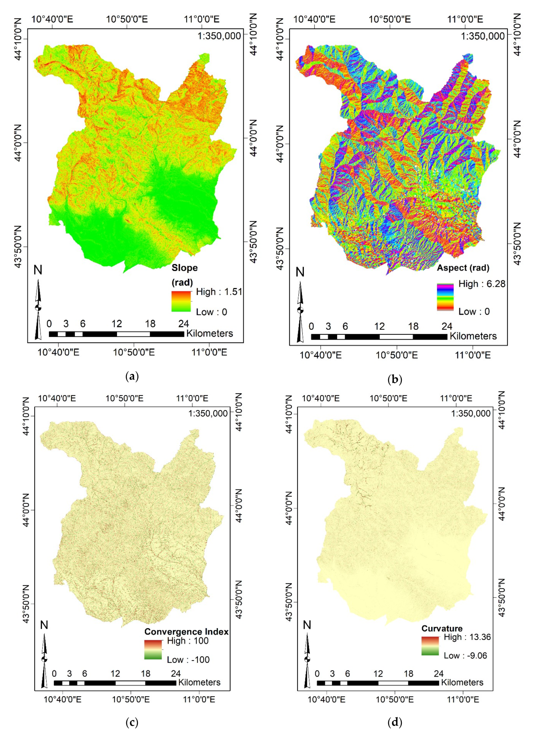
The review of the literature and the data already collected have led to identifying an amount of 29 potential input features, including 9 topographical-based features (Elevation, Aspect, Slope, Convergence Index (CI) [112], Curvature, Vector Ruggedness Measure (VRM) [113], Topographic Position Index (TPI) [114], Topographic Ruggedness Index (TRI) [115], and Slope Length (SL) [116]), 4 hydrological factors (Stream Power Index (SPI) [117], Topographic Wetness Index (TWI) [118], River Density, and Average Cumulative Yearly Rainfall), 4 environmental-based factors (Direct and Diffusive Yearly Solar Radiation [119], Wind Exposition (WE) [119], and Earthquake Susceptibility), 2 social system-based factors (Land Use and Area Type), 4 susceptibility-based factors (Landslide Susceptibility, Flood Susceptibility, Erosion Susceptibility, and Drainage capacity of the soil), and 4 subsoil composition-based factors (sand, silt, clay, and organic content). Distance from Rivers and Landslides have also been computed.
Apart from the sixteen features collected (Figure A1, Figure A2, Figure A3 and Figure A4) and inserted directly into the models, several others require to be determined through the GIS platforms. Both SAGA-GIS and ArcGIS have allowed computing most of them by specific instructions. They are based on mathematical relations (such as for the calculation of Aspect, Slope, Curvature, CI, TPI, TRI, SL, SPI, TWI), geospatial interpolations (such as for the computation of River Density, Average Cumulative Yearly Rainfall, Earthquake Susceptibility, Distance from Rivers, and Distance from Landslides), or more complex procedures (such as for the definition of the VRM, WE, Direct and Diffusive Solar Radiation). Figure A5, Figure A6 and Figure A7 report the computed topographical factors, hydrological factors, and environmental factors, respectively. Finally, Figure A8 shows the map of the distance from rivers and distance from landslides, respectively.
ArcGIS software has been used for computing the following input features:
  • Aspect and Slope (exploiting the Elevation) by their homonymous commands;
  • Average Cumulative Yearly Rainfall (considering the rain gauges localization and rainfall data) and the Earthquake Susceptibility (considering the earthquakes localization and magnitude) using an ordinary spherical kriging interpolation [2,58,61];
  • Distance from Rivers and Distance from Landslides by the Euclidean Distance command (considering the landslides localization and the river network);
  • River Density through the Kernel Density command (using the river network as input).
  • Furthermore, SAGA-GIS software has been exploited for deriving:
  • CI, Curvature, VRM, TPI, TRI, SL, WE, Direct and Diffusive Solar Radiation by their homonymous commands (considering the Elevation);
  • SPI, TWI, by their homonymous commands (considering the Slope and the catchment area derived from the Elevation).
In order to solve the semantical relations between features, a raster-based grid format with a 10-m spatial resolution has been used for all the predictors.
The main analytical relations for computing the features obtainable through a single relation, i.e., CI, TPI, TRI, SL, SPI, and TWI (Equations (1)–(6)), are reported below. The reader is referred to the references proposed for the calculation of the remaining more complex input features.
  • CI:
    C I = [ ( 1 n ) i = 1 n ϑ i 90 ° ] · 10 9
    where ϑ i describes the angle between the aspect of the i-th surrounding neighbor cell and the center cell (the cell under analysis) and n is the number of neighbors (eight neighbor cells considering a 3-by-3 scheme);
  • TPI:
    T P I = z 0 1 n R i R z i
    where z 0 is the elevation of the cell under analysis, z i is the elevation of the surrounding cells within a specified radius (100 m), and n R is the number of cells surrounding z 0 ,
  • TRI:
    T R I = i , j n ( z i , j z 0 )
    where z i , j is the elevation of each neighbor cell (eight neighbor cells considering a 3-by-3 scheme) to the elevation z 0 of the center cell (the cell under analysis);
  • SL, SPI, and TWI:
    S L = ( S 22.13 ) 0.6 · ( sin ( α ) 0.0896 ) 1.3
    S P I = S · tan ( α )
    T W I = ln ( S tan ( α ) )
    where S is the specific area of the catchment (expressed as m2/m of catchment) and α is the slope gradient (expressed in degrees). Equation (4) shows that SL is computed by knowing information on catchment area and slope; SAGA-GIS computes them internally by exploiting the Elevation.
It is worth reminding that:
  • Slope represents the rate of change of the surface in horizontal and vertical directions from the cell under analysis;
  • Aspect defines the slope direction. The values of Aspect of a cell indicates the compass direction (expressed in [rad] in the present paper) that the slope faces at that cell;
  • Curvature is equal to the second derivative value of the input surface (the Elevation). For each cell, a fourth-order polynomial function is fit to a surface composed of a 3-by-3 window;
  • VRM computes terrain ruggedness by measuring the dispersion of vectors orthogonal to each cell of the terrain input surface (Elevation). The cell under analysis and the eight surrounding neighbors are decomposed into three orthogonal components exploiting trigonometric relations, slope, and aspect. The VRM of the center cell (the cell under analysis) is equal to the magnitude of the resultant vector. Finally, the magnitude of the resultant vector is divided by the number of neighbor cells and subtracted from 1 (standardized and dimensionless form). Therefore, VRM ranges from 0 (flat) to 1 (most rugged) [120];
  • WE is represented by the absolute angle distance between the aspect and the azimuth of wind flux considering the North direction as the reference. It considers surface orientation only, neglecting the influence of surrounding terrains as well as the slope. Accordingly, WE moves from 0° (windward) to 180° (leeward). In the present paper, it is expressed in its dimensionless form (i.e., values lesser than 1 define wind shadowed areas whereas values greater than 1 identify areas exposed to wind). Considering that the predominant wind directions were not known in advance, the averaged WE has been computed by imposing several hypothetic directions (i.e., for each 15°) [119];
  • Direct Solar Radiation received from sun disk ( S d i r ) and Diffuse Solar Radiation received by the sky’s hemisphere ( S d i r ), on an unobstructed horizontal surface, in clear-sky conditions, at an altitude z , can be computed by Equations (7) and (8) exploiting the Elevation data [119]:
    S d i r = sin ( θ ) · S c · e z l · Δ z sin ( θ )
    S d i f = 0.5 · sin ( θ ) · S c · c · ( 1 e z l · Δ z sin ( θ ) )
    where S c is the solar constant ( ~ 1.367 kW/m2), l is the air density integrated over distance Δ z from top of the atmosphere to the elevation z , and c < 1 is a coefficient for accounting the loss of absorbed exo-atmospheric solar energy when passing the atmosphere (in the present study, c = 0.7 ).
Table 2 shows the descriptive statistics of the numerical features, in terms of the unit of measure (Unit), an example reference in which the same input has been used (Ref.), the minimum, maximum, and mean value (Min., Max., and Mean), the standard deviation, skewness, and kurtosis (St. Dev., Skew., and Kurt.).
Table 3 describes the categorical features in terms of type, i.e., Ordinal (Ord), Categorical (Cat), or Binary (Bin) feature, and the number of categories.

3.3.3. Output Target Response

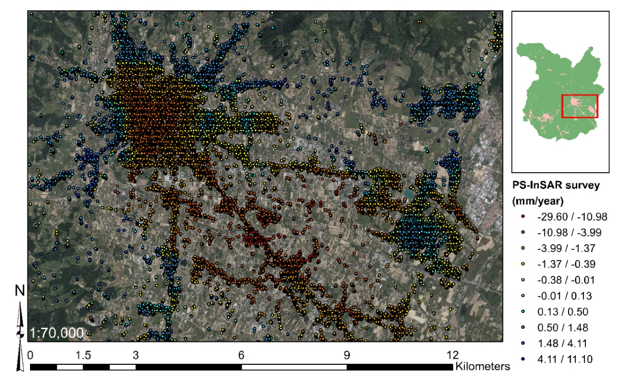
The MLAs are calibrated for predicting surface motion ratio in terms of mm/year. This considering, we have exploited the measurement of 52,257 PS detected over the study area (Figure 4a). The PSs with a coherence greater than 0.9 have been considered for ensuring the reliability of their measurements. The average velocity of each PS is considered as the target response of the MLAs. It is possible to note in Figure 4b that most PSs are localized over both urban areas and infrastructures that cross the study area.
The interferometric process is repeatedly carried out by the TRE Altamira (https://site.tre-altamira.com/), Milan, Italy, every six days, and provided free of charge by the “Geoportale Lamma” website https://geoportale.lamma.rete.toscana.it/difesa_suolo/#/viewer/openlayers/326. Indeed, the Tuscany Region is the first worldwide example of a regional scale monitoring system based on continuous satellite interferometric data processing, and in Reference [121], the main characteristics of the project are explained. In the present study, TRE Altamira has exploited a stack of co-registered Sentinel-1 ascending orbit acquisitions that cover a period from 12 December 2014 to 24 August 2019. The stack is composed of 210 images. The subsidence effect reaches an intensity of 29.6 mm/year, while uplifts assume maximum values equal to 11.1 mm/year.
It is worth considering that the surface motion revealed by PS-InSAR should be verified using external ground truth information, such as Global Navigation Satellite System (GNSS) measures. As for the Province of Pistoia, the issue of subsidence phenomenon is widely known and recognized by several international studies. There are some researches focused on validating the PS-InSAR data using GNSS information. For instance, in Reference [17], PS-InSAR data obtained by Sentinel-1 acquisitions from 2014 to 2017 have been compared and validated with GNSS data for the Province of Pistoia; the Authors reported that the difference in the vertical displacements detected by the Sentinel-1 data before and after the GNSS correction in Pistoia Province is approximately 1.0 mm/year. Supported by these findings, we can consider surface motion observations reliable enough to be used in the modeling of the MLAs.
As described in Section 3.1, the city of Pistoia is strongly affected by surface motion phenomena: at the city center, there are strong subsidence effects, while uplift motions have been detected at the boundaries of the city. Figure 5 demonstrates that the PS-InSAR technique can reveal such surface movements.

3.3.4. Definition of the Training and Test Sets

It is essential to identify the training and test set before move on to the training phase of the MLAs. In the present study, it has been chosen to randomly separate the dataset in the training set and test set, with a split percentage of 70% and 30%, respectively. Indeed, such percentages are generally employed. Several authors implemented the 70/30-based split in their modeling [59,61,72,83,85,94,101]. Once the random split has been implemented, the training set consists of 36,580 PS-InSAR observations, while the test set consists of 15,677 PS-InSAR observations.
It is also worth mentioning that the training set contains a validation set, according to a 10-Fold CV procedure.

3.4. Feature Selection Approach

Feature selection is a critical step in data preprocessing for alleviating overfitting issues of MLAs and reducing their complexity significantly (improving their interpretation) and the computational cost for their training. Indeed, some of the input features may be highly correlated or even redundant Moreover, a feature selection approach should lead to better MLAs in terms of predictive performance. A comprehensive overview of feature selection approaches and tutorial for their implementation can be found in Reference [122]. The present study focuses on methods called “wrapper approaches”, considering that they propose automatic strategies for recognizing the essential features of a dataset.
The wrapper feature selection approach has been introduced in Reference [123]. Wrapper-based approaches involve a robust but straightforward and pragmatic procedure for challenging the issue of feature selection. They are not directly connected to the algorithm to be trained, and they are inserted as an independent phase before the training step. Indeed, the wrapper procedure has to be carried out before the training phase of whatever MLAs. Therefore, it is one of the essential steps in the dataset preparation phase.
Approaching a feature selection by a wrapper-based approach means computing the performance of a prefixed MLA trained by several subsets of input features. The aim is to discover the subset of input features that shows the highest performance. The procedure is iterative and completely automatic. Unfortunately, wrappers suffer from the curse of dimensionality; in order to alleviate such issues, some search strategies can be followed, e.g., forward, backward, and bi-directional feature selection are efficient strategies [122,124]. In the forward approach, starting from a predetermined subset (generally starting with an empty subset of predictors), the predictors are inserted progressively one after the other (one for each iteration). In the Backward approach, the procedure is quite similar but works in the opposite direction. Still, starting from a predetermined subset (generally starting with the use of all the predictors), the predictors are removed progressively one after the other. Finally, in the bi-directional approach, at each iteration, the predictors can be both added and removed.
The use of wrapper feature selection approaches is not very common in environmental modeling, perhaps for its computational cost. We found an example of using a forward and backward feature selection approach as data preprocessing in Reference [96], where SVM, ANN, and GP have been used for predicting surface settlements after metro tunnel excavations.
In the present study, forward, backward, and bi-directional wrapper approaches have been implemented. Forward and bi-directional wrappers started with no attributes. Backward wrapper started with all the attributes. Each wrapper exploited a 500-RT-based RF as a learning algorithm. The predictive performance has been evaluated by RMSE after a 5-Fold CV process. It was defined that the wrappers should have stopped if, after 5 iterations, an improvement in RF performance was not identified.

3.5. Machine Learning Algorithms

Considering that we aim to predict surface motion ratio in terms of mm/year relying on a set of already known observations (i.e., we know in advance input and target output to be modeled), supervised MLAs for regression are the most suitable tools for achieving our purpose. Once trained, they can be used to make predictions on new data (i.e., on the samples belonging to the test set for evaluating the predictive performance) or on samples whose target response is not known (i.e., mapping the surface motion even in those places in which PS are not available).
The software MATLAB R2019b and Waikato Environment for Knowledge Analysis (WEKA) 3.8.4 [125,126] have been used to carry out the modeling. Modeling was performed on a workstation with the following configuration:
  • CPU: Intel Core i9-9900 (8 core, 16 threads, 3.10 GHz, max 5 GHz);
  • GPU: NVidia GeForce RTX 2080TI-11GB;
  • SSD: Samsung 970 PRO 512 Mb;
  • RAM memory: Corsair Vengeance LPX 32GB DDR4 3000 MHz (2 × 16 GB).
The following subsections report the core ideas and references of each MLA implemented in the present study.

3.5.1. Regression Tree

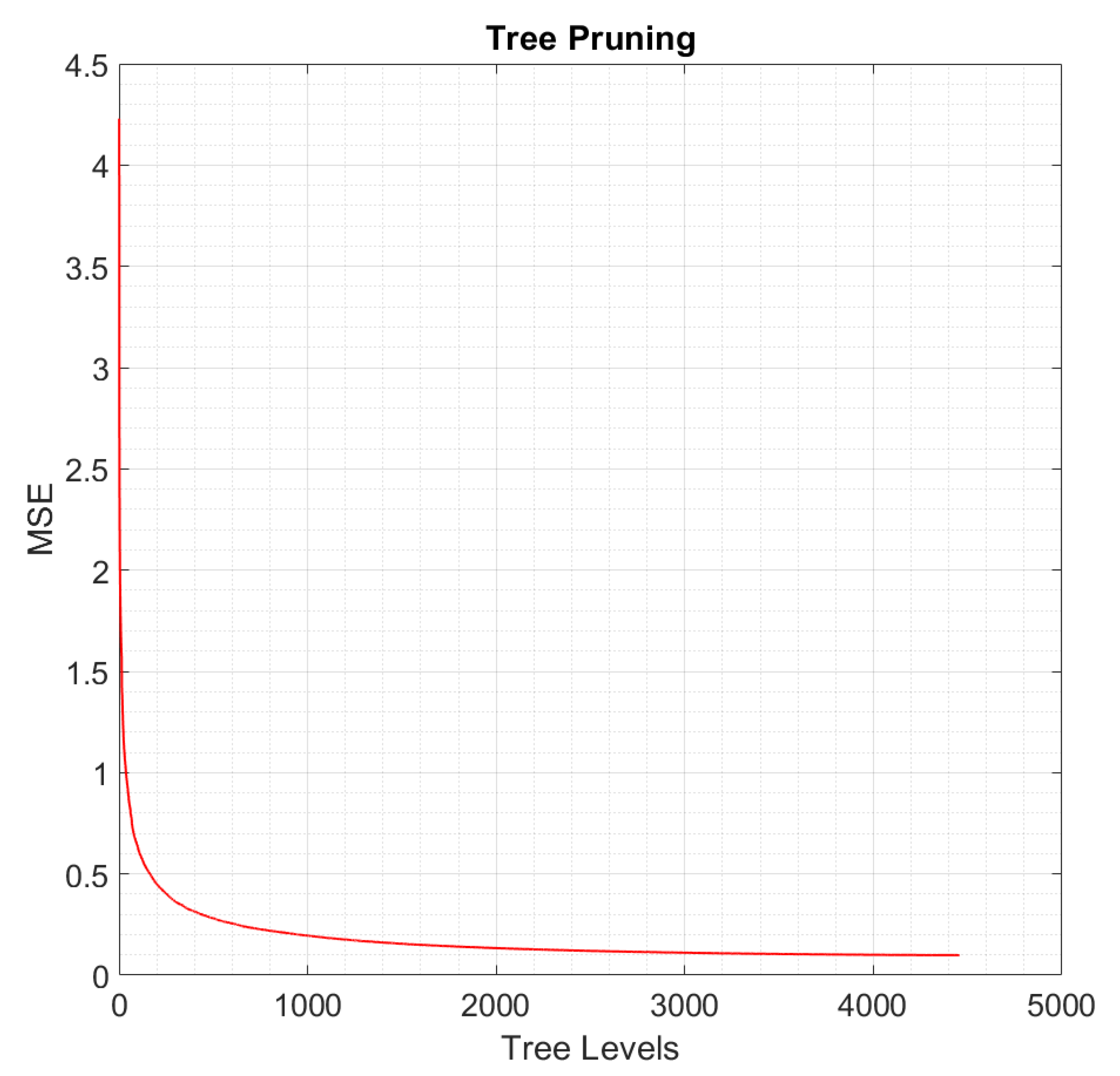
Breiman developed the RT algorithm in 1984 [127]. Commonly, the name of such an algorithm is Classification and Regression Tree (CART), considering that it can be employed both for classification and regression tasks, depending on the output target. In the present paper, we used the name “RT” since we are dealing with the construction of a CART that aims to predict a continuous target output. The RT algorithm is a hierarchical supervised learning algorithm made by decision rules that iteratively divides input features into homogeneous zones, called nodes. Such decision rules are learned from the training samples automatically by inference. Once the RT is trained, a tree-based graph is defined. The first node of the tree graph will be called the root node, while at the end, nodes will be called leaf nodes. The decision rules belonging to each node can be used for making predictions by using new unknown data. In this paper, we used a binary RT, i.e., each node (from the root node to the leaf nodes) has been subdivided into two branch nodes according to a specific decision rule. The Recursive Partitioning (RP) algorithm [127,128] has been exploited for defining the decision rules of each node. The leading analytical relation for training the RT can be found in the tutorial of Torgo [129]. Once a decision rule is defined for a node, the RP has been applied again to both child nodes. A termination criterion establishes when the RP process has to conclude. If the RP is not to be applied, the node is defined as a leaf node; the predicted value of the target output is the average value of all the y i included in the leaf node. In this study, a MSE threshold equal to 10 6 represents the termination criterion to be satisfied. This “relaxing” value should lead to a deep and complex tree that accounts for all the hidden patterns between features; it has been chosen considering that a subsequent pruning procedure should simplify enough the RT for preventing overfitting. To prune the RT, the so-called Pruning Level (PL) has to be fixed. PL is the number of hierarchical levels that have to be pruned. There is not rule of thumb for identifying the right PL. One procedure is to compute the Resubstitution Error (MSE) on the validation set for different PL and find the place in which adding nodes does not significantly increase the accuracy of the model.
Four hyperparameters have to be tuned: the fixed number of the input feature random sample for identifying the decision rules of the RT, the maximum number of splits, the minimum leaf node size, and the minimum parent size for each child node. Section 3.6 and Section 3.7 describe how they have been defined in our study.

3.5.2. Support Vector Machine

The concept of SVM was introduced under the name of the generalized portrait method by Vapnik and Lerner in 1963 [130]. Subsequently, through the definition of the statistical learning theory, Vapnik developed the current form of SVM [131,132,133,134]. In that form, SVM has been firstly implemented for classification purposes. Afterward, through the studies of Smola and Vapnik [135,136], the concept of SVM has also been extended to regression tasks. The general basic idea of SVM is to map the original data χ into a feature space with high dimensionality through a non-linear mapping function and then construct an optimal hyperplane in such a new feature space. In the case of classification tasks, SVMs search for an optimal hyperplane that maximally separates the data into two classes. On the contrary, in the case of regression tasks, the hyperplane to be searched for lies close to as many points as possible.
Considering the target output of the present study, the SVM for regression has been implemented. Valuable tutorials on the implementation of SVM for regression can be found in References [97,137]. The leading analytical relations can be found in such studies. For the sake of brevity, we just mention that an SVM for regression is generally called ε -insensitive SVM [131] since the aim is to discover the optimal hyperplane by minimizing the following ε -insensitive loss function:
L ε ( y ) = { 0                           f o r   | f ( x ) y | ε | f ( x ) y | ε           o t h e r w i s e
It is proved [97,137] that the function f describing the optimal hyperplane is:
f ( x ) = i = 1 l ( α i α i * ) x i , x + b
where α i , α i * are non-negative constants obtained by exploiting a Lagrange function to solve a convex optimization process concerning the minimization of L ε ( y ) . Therefore, the hyperplane to be searched for only depends on dot products between observations x i . When a non-linear relation links input features and target output, the SVM can solve the issue by mapping the input features into a high-dimensional feature space through some non-linear kernel functions [133]. The concept of the so-called kernel trick is essential to reduce dramatically the computational cost required for training the SVM [131]. In the case of the present paper, the radial basis kernel function (or Gaussian kernel) [138,139] has been implemented for mapping the feature into a high-dimensional feature space able to account for the non-linear relations between output response and input features (Equation (11)).
K ( x i , x j ) = e x i x j 2 2 σ 2
Three hyperparameters have to be tuned in the present study: the Box Constraint C (it defines the trade-off between the flatness of f and the amount up to which errors higher than ε are accepted), the value of ε , and the value of Gamma γ = 1 2 σ 2 for the computation of the kernel trick. Section 3.6 and Section 3.7 describe how they have been defined.

3.5.3. Random Forest

The RF algorithm has been defined in the study of Breiman [140]. RF belongs to the family of ensemble learners, which are algorithms composed of a large number of single learners, whose predictions are provided by aggregating the single prediction of each learner in some way. As for the previous algorithms, RF can be implemented for solving classification or regression problems. In the case of RF for regression, the “forest” consists of a massive number of uncorrelated RTs that operate as an ensemble learner. The fact that these RTs are uncorrelated is the core of the algorithm and its main strength. Indeed, in addition to each advantage of the RT algorithm, RF should not be prone to overfit the data, and it should be less sensitive to changes in the training set. Besides, no pruning process is required. In order to develop the uncorrelated trees:
  • RF algorithm exploits the bootstrap aggregation (also called Bagging) process, i.e., it defines several subsets of training samples with replacement, and then uses each of them for training each RT. For each subset, RF exploits two-thirds (in-bag samples) for training the RTs, and the remaining one-third (out-of-bag samples) for a CV process. This CV process is followed by the RF to minimize the error estimation (out-of-bag error) and define a robust algorithm;
  • RF exploits the feature randomness approach, which is to choose a fixed number of input features randomly chosen to be used for defining the decision rules of each RT. Accordingly, each RT is trained by a different subset of input features. They have a high variance in their prediction and a low bias.
Once trained, RF for regression can make predictions using new data by averaging the predicted target output that each RT predicts. Therefore, RF computes the arithmetic mean of all predictions, i.e., each RT has the same weight.
Two hyperparameters have to be tuned:
  • The amount of RT structures constituting the forest: RF is not prone to overfit the data, then the number of decision trees can be enormous in order to enhance its performance. However, the higher the number of RT to train, the higher is the computational cost required for growing the RF. Moreover, the accuracy of RF does not significantly improve once a certain number of RT has been reached;
  • The fixed number of input factors randomly sampled as candidates at each split.
Section 3.6 and Section 3.7 describe how they have been defined in this study.

3.5.4. Boosted Regression Tree

As for the RF, BRT is an ensemble learner based on tree aggregating. Nonetheless, instead of training parallelly, many uncorrelated trees are averaged to avoid overfitting only at the end of the process, and in the BRT algorithm, RTs are added sequentially to the ensemble. Therefore, Boosting is sequential: it is a forward, stage-wise procedure [141]. At each iteration, the new RT to be added concentrates expressly on those samples that are accountable for the remaining regression error [142] (the samples that result in the higher residuals).
The boosting technique has been introduced in Reference [143], then it has strongly imposed itself in Machine Learning modeling by the definition of the AdaBoost algorithm [144], where the authors defined a boosting algorithm composed of a collection of CART for solving classification problems. Boosting techniques for regression tasks appear firstly in References [145,146,147], in which authors employ a gradient descent process in order to minimize a specified loss function. A squared loss function is usually employed for regression purposes. Generally speaking, at each iteration, an additional RT is trained on the residuals of the previous iteration, and it is added to the ensemble. At the end of the process (once the number of RT composing the BRT, N R T , is reached), the final prediction T ( x i ) is computed as:
T ( x i ) = T 1 ( x i ) + η k = 2 N R T T k ( x i )
where T 1 ( x i ) is the prediction of the first RT and η is the learning rate. The process is stage-wise, i.e., the existing RTs are left unchanged as the model is enlarged. A detailed explanation of how the BRT algorithm works can be found in References [141,142,148].
Three hyperparameters need to be tuned in BRT: the number of learning cycles N R T , the learning rate η , and the minimum size of the leaf nodes. As for the other MLAs, in Section 3.6 and Section 3.7, readers can find a description of how they have been defined.

3.6. Hyperparameter Tuning by Bayesian Optimization Algorithm

Before starting the training phase of the MLAs, in which the model parameters can be discovered, one has to specify a set of hyperparameter values that allow reaching the highest performance during the training phase. This step constitutes an optimization problem where the function f (i.e., the objective function f that aims to represent the distribution of the hyperparameters) to be optimized is commonly unspecified. The BOA [149] is an efficient optimization algorithm for solving this kind of optimization problem since it is an automatic process, it does not require any manual search of the hyperparameters (an issue in manual tuning), and it does not suffer from the curse of dimensionality (an issue in Grid and Random search). BOA can solve functions that are computationally expensive to find the extremes values and can be applied for solving functions that do not have a closed-form expression, functions which are expensive to calculate, functions whose derivatives are hard to compute, and nonconvex functions. Some comprehensive tutorials on BOA implementation can be found in References [150,151].
Employing the Bayes theorem, BOA combines prior information about the unknown function f with sample information in order to obtain posterior information of the function distribution. Then, relying on this posterior information, BOA can deduce where the function has the optimal value. It is generally assumed that the Gaussian Process [152] is suitable as the prior distribution of f [151]. Accordingly, at each iteration, BOA exploits Gaussian Process for fitting the sample data and update the posterior distribution. By exploring the hyperparameters space, the aim is to compute the value of an unknown function f ( x ) at several sampling points to find the one where it is maximized:
x + = max x Ψ f ( x )
where Ψ denotes the search space of x (i.e., Ψ is the hyperparameter space, and x is a vector of values that define the values of the hyperparameters). In order to identify x + , BOA exploits the Bayes’ theorem:
P ( M | E ) = P ( E | M ) P ( M )
where P ( M | E ) is the posterior probability of a model M (in this case, M represents the behavior of f ( x ) ) given the data evidence E (in this case, E is the training sample point used for discovering the hyperparameters), P ( E | M ) is the likelihood of observing E given the model M , and P ( M ) is the prior probability of M , assumed that it follows a Gaussian Process.
Equation (14) highlights the key step of BOA: combining the prior distribution of f ( x ) with a sample point (the evidence E , i.e., at the beginning of the BOA, a set of evaluations of the function f ( x ) is identified by imposing different random values of the hyperparameters) to compute P ( M | E ) . Consequently, the posterior probability is used to find where the function f ( x ) can be maximized by the selection of an appropriate x + according to a specific criterion. The criterion is represented by the minimization of a utility function u , generally called the acquisition function. By the minimization of the function u , BOA identifies the next sample point (i.e., the next vector x to be added to the training sample). In the present paper, since we are dealing with MLAs for regression, the acquisition function of the i-th iteration is defined as:
u i = log ( 1 + l o s s i )
where l o s s i is the average cross-validated error (MSE) of the algorithm trained by using the set of hyperparameters defined at the i-th iteration committed on the folds not used for training the algorithm.
Therefore, BOA implements the following steps:
  • A set of evaluations of the function f ( x ) (training sample) is identified by imposing a Gaussian Process distribution and five random values of;
  • The acquisition function is computed; the BOA identifies the next sample point x that could improve the acquisition function and adds it to the training sample;
  • The BOA updates the posterior distribution and computes the acquisition function again;
  • At each new iteration, steps 1–3 are repeated, updating sequentially the P ( M | E ) with one new sample point x per iteration; at each iteration, a new sample point x is found and added to the training sample (the evidence data).
Once a fixed number of iterations is completed, the BOA concludes its process. The sample point x that demonstrates the best performance is chosen as x + of the algorithm. Therefore, the hyperparameters are identified. Each iteration of the BOA can take from a few seconds to several hours of work. In this study, each MLA was optimized with 30 iterations of the BOA.

3.7. K-Fold Cross-Validation Procedure

CV is a well-known and established process for training an algorithm, assessing its performance, or comparing the performance of different sets of hyperparameters for a chosen MLA [153]. Historically, the CV strategy has been conceptualized in Reference [154] by Larson. CV is meant as the action of splitting the dataset into two parts; the first one to be used for training the algorithm, while the second one to be used for assessing the performance of the modeling. Subsequently, the structure of k-fold CV has been defined in Reference [155], where the training set is divided into k folds of the same size. Accordingly, there are k iterations of the procedure. At each iteration, k-1 folds are used for training the algorithm, while the remaining fold is used for the validation phase. Therefore, in a CV procedure, each observation is used both for training and for testing. In Reference [156], Kohavi recommended a 10-fold CV as the best model selection procedure. Indeed, several other studies [60,67,69,73,86,87] used k-fold CV.
In this paper, a 10-Fold CV procedure has been implemented for each i th iteration of the BOA in order to evaluate the performance of the i th training phase of the MLAs (i.e., the MLAs trained by the i -th set of hyperparameters identified by the BOA process).

3.8. Predictor Importance

A tree-based model can compute the importance of each input factor used in training the MLAs. The computation of the Predictor Importance (PI) should demonstrate how much the target output of the MLAs is related to each input factor; the higher is the PI, the higher is the degree of the link between a specific input and the target output. Nonetheless, it worth mentioning that the term “Importance” is also connected to the splitting process of the tree-based model. Therefore, if the input is chosen early for splitting a node compared to another input, it gains more PI, even if this input is not strongly linked to the target output. Therefore, the PI values should be judged carefully.
The analytical relations for computing the PI are reported below. A detailed description of the procedure can be found in References [140,157]. As said in the description of the RT, a tree, T, is trained by a sample of N observations, exploiting the RP algorithm [127,128]. RP recognizes at each node, t, the best split, s t , for subdividing the node observations, N t , into two subsamples (the branch nodes), t L and t R ; RP aims to maximize the decrease Δ i ( s t , t ) of an impurity measure, i ( t ) . RP concludes its process when nodes become homogeneous (i.e., every observation belongs to the same class or the difference between target values is lower than a minimum MSE threshold). The impurity decrease is computed using Equation (16):
Δ i ( s t , t ) = i ( t ) p L i ( t L ) p R i ( t R )
where:
  • P L = N t L / N t
  • P R = N t R / N t
In the present study, the impurities i(t), i ( t L ) , i ( t R ) , at the nodes t, t L , t R , are represented by the MSE of the samples belonging to such nodes, respectively. Considering the feature randomness procedure and the ability to exploit a high number of uncorrelated trees, a 500 tree-based RF algorithm has been used for computing the PI. Following the study of Breiman [140], the PI of an independent input feature, X m , can be computed as:
P I ( X m ) = 1 N T T t T : v ( s t ) = X m p ( t ) Δ i ( s t , t )
where:
  • N T is the number of trees composing the forest;
  • t are the nodes belonging to the tree T ;
  • p ( t ) Δ i ( s t , t ) are the weighted impurity decreases;
  • P I ( X m ) is the importance of the input feature X m
  • p ( t ) is the proportion N T / N of samples reaching the node t;
  • v ( s t ) is the independent variable used in split s t .

3.9. Goodness-of-Fit and Predictive Performance Evaluation

The MLAs have been evaluated by three performance metrics: R2, RMSE, and MAE. They can be computed by the following Equations (18)–(20):
R 2 = 1 i = 1 N ( Y i p r e d i c t e d Y i o b s e r v e d ) 2 i = 1 N ( Y i o b s e r v e d Y ¯ o b s e r v e d ) 2
R M S E = 1 N i = 1 N [ ( Y i p r e d i c t e d Y i o b s e r v e d ) ] 2
M A E = 1 N i = 1 N | Y i p r e d i c t e d Y i o b s e r v e d |
where:
  • Y i p r e d i c t e d is the i-th predicted value of the target output Y ;
  • Y i o b s e r v e d is the i-th observed value of the target output Y ;
  • Y ¯ o b s e r v e d is the averaged observed value of the target output Y .
The coefficient R2 describes the ratio of explained variance by the model, comparing the sample variance of the model and that of the reference population. The RMSE represents the standard deviation of the residuals, i.e., the distribution of the difference between predicted and observed values. Therefore, RMSE shows the accuracy of the predictions. Moreover, MAE provides a measure of the average dimension of the errors.
Moreover, the scatterplots have been computed for each algorithm in order to compare observed and predicted values. The scatterplots enable identifying quickly if the training and testing phases have been conducted correctly, and if the algorithms are both able to represent the observed samples (training) and make predictions on new data (test). Furthermore, scatterplots are worthwhile tools for the identification of potential clustering of the points and outliers. Therefore, scatterplots should be more informative than the R 2 since the latter provides only a concise summary of the linear relationship between observations and predictions, while scatterplots provide a visual summary of a linear or nonlinear association [158].
Finally, in order to compare the MLAs, we compute the Taylor Diagram. As the name suggests, this tool has been defined by Taylor [159,160], and it suggests a concise and graph-based metric to assess the overall performance of an algorithm and enables an objective comparison among several models. In the Taylor Diagram, the standard deviation, the RMSE, and the R 2 of each MLA implemented and those of the reference population are included. The graph has to be read “radially”. In the present study, the standard deviation is represented by black arches, the RMSE by green arches, and the R 2 by blue arches. Finally, the performance of the MLAs is represented by red dots of various shapes. The MLAs that lies the most near the performance of the reference population (i.e., the red dot which belong R 2 = 1, RMSE = 0, and standard deviation = 2.09 mm/year) are the most representative. An example of a Taylor Diagram implementation for ML-based environmental modeling assessment can be found in Reference [101].

4. Results and Discussion

4.1. Feature Selection

The following Table 4 reports the outcomes in terms of the selected subsets of input features of the wrapper feature selection approaches. The starting set, the number of iterations, and the RMSE of each wrapper are also reported. The wrappers are based on a 500-RT-based RF.
From Table 4, we can appreciate that the three approaches lead to very similar results. Indeed, a set of input features is repeated over the three wrappers: this set includes Elevation, Rainfall, Distance from rivers, Distance from landslides, Earthquake susceptibility, Type of area, River Density, and Silt content of the subsoil. Moreover, the other relevant features elected by all the wrapper are those related to the subsoil composition (Sand, Organic, and Clay). Silt is considered relevant by all the wrappers). Specifically, Sand is elected by Forward and Bi-directional wrapper, Clay is elected by the Backward wrapper, and Organic by the Forward wrapper. The RMSE is very similar in all three approaches. The Backward wrapper shows the lower one and, therefore, the subset of feature selected by this approach has been chosen as the set of input features of the MLAs.

4.2. Machine Learning Hyperparameters

The following lists report the hyperparameters of the MLAs tuned by BOA and 10-Fold CV. Moreover, the time for training algorithms is reported.
RT:
  • CV process: 10-Fold;
  • Optimization of the Hyperparameters: Bayesian Process, 30 iterations;
  • Time for training the CART: 90 s;
  • Fixed number of random variables to choose for splitting nodes: 9;
  • Maximum number of splits: 8330;
  • Minimum leaf nodes size: 2;
  • Minimum parent size: 10;
  • Split criterion: MSE;
  • Number of nodes: 12,995;
  • Number of tree levels: 4457;
  • Number of pruned levels: 2000 (according to Figure 6, if the RT is pruned by 2000 levels, the MSE does not increase significantly and the resulting RT is less complex and less prone to overfit data);
  • Number of nodes after tree pruning: 6705 (2257 resulting tree levels).
SVM:
  • CV process: 10-Fold;
  • Optimization of the Hyperparameters: Bayesian Process, 30 iterations;
  • Time for training the SVM: 60,200 s;
  • Standardize the input factors: yes;
  • Type of kernel function: Gaussian kernel;
  • C (Box constraint): 38.361;
  • Gamma: 0.4017;
  • Epsilon: 0.0012.
RF:
  • CV process: 10-Fold;
  • Optimization of the Hyperparameters: Bayesian Process, 30 iterations;
  • Time for training the RF: 997 s;
  • Fixed number of random variables to choose for splitting nodes: 9;
  • Number of trees: 483;
BRT:
  • CV process: 10-Fold;
  • Optimization of the Hyperparameters: Bayesian Process, 30 iterations;
  • Time for training the BRT: 4285 s;
  • Fixed number of random variables to choose for splitting nodes: 9;
  • Number of learning cycles: 248;
  • Learning rate: 0.1042;
  • Maximum number of splits: 1470;
  • Minimum size of the leaf nodes: 6;
We can note that the RT algorithm shows the lowest time for training (90 s), followed by RF (997 s), BRT (4285 s), and SVM (60,200 s). If the training time is relevant for the practitioners, then the SVM should be avoided since it requires about 700 times more time than RT for its training. RT and RF could be an efficient solution in this case. If the number of tunable hyperparameters is essential instead, then the RF is the most efficient algorithm, considering that it requires two hyperparameters only. On the contrary, RT requires that several hyperparameters have to be tuned, and also the pruning process must be performed to avoid overfitting. If there are no limitations due either to the training time or to the number of hyperparameters to be tuned, then a suitable strategy is to train all the MLAs and check which of them has the best performance.

4.3. Goodness-of-Fit and Predictive Performance Assessment

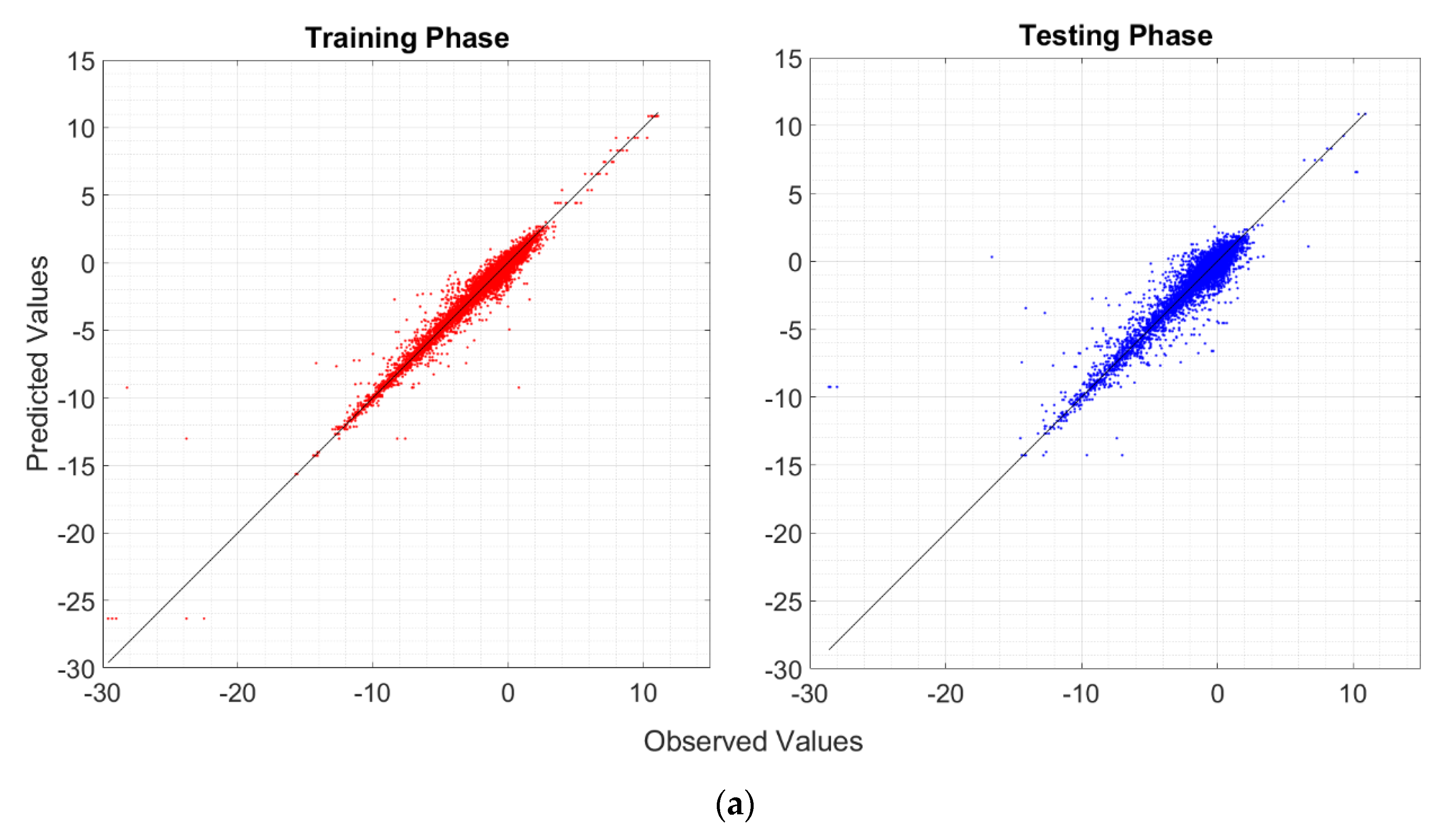
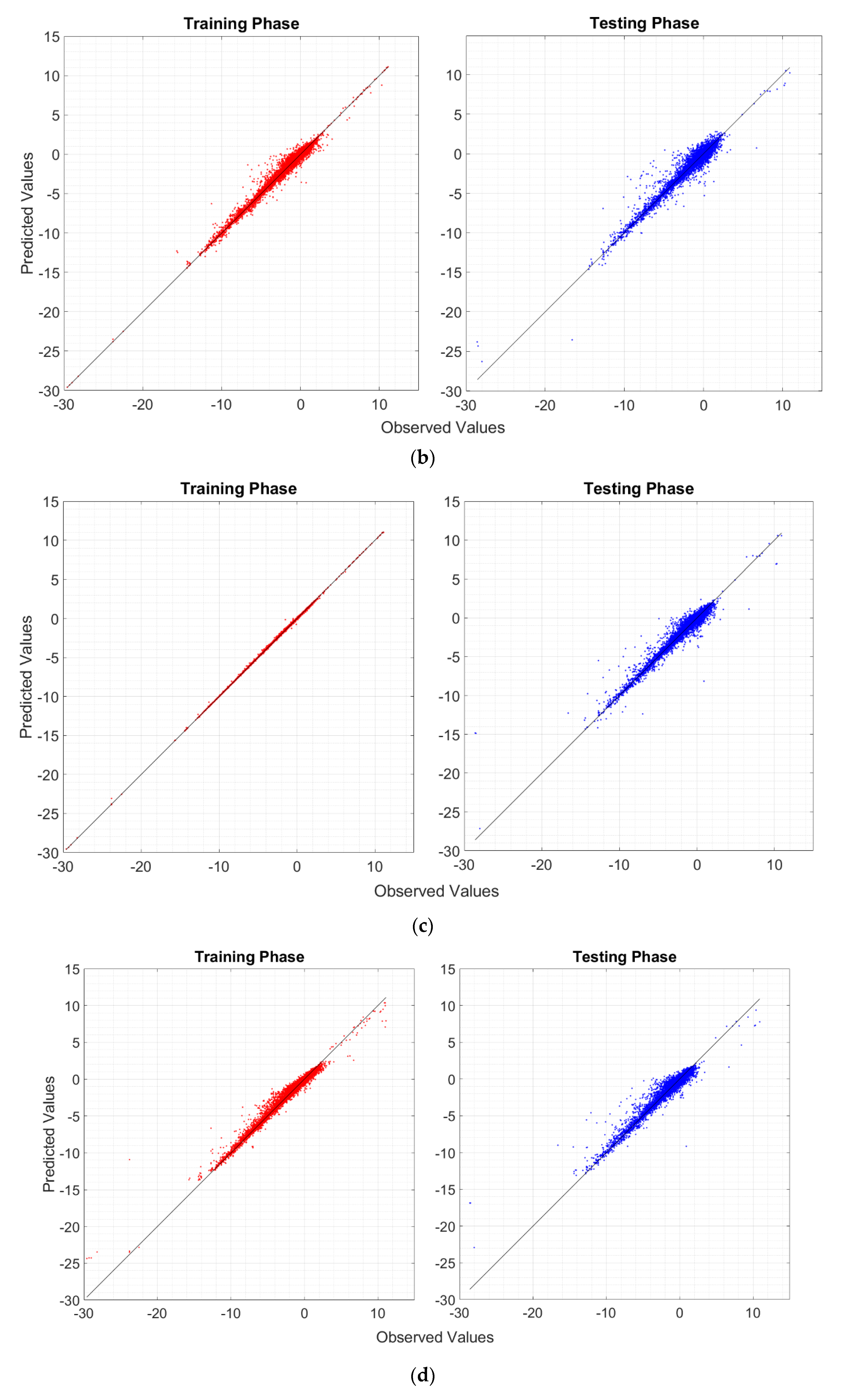
This subsection reports the performance of the MLAs in both training and test phases. Firstly, through the computation of the Standard Deviation, R2, RMSE, and MAE, the performance of the algorithms, i.e., the Goodness-of-Fit (training) and the Predictive Performance (test), can be observed by concise numerical metrics (Table 5). Subsequently, the scatterplots of each MLA, both in the training and test phase, have been reported (Figure 7). The scatterplots provide information related to the presence of outliers, clustering, overfitting, and potential non-linear relations between observed and predicted values. Finally, the Taylor Diagram is reported for comparing the Predictive Performance of the MLAs (Figure 8). Through this graph, we can compare the MLAs and check which of them are the most reliable for making predictions.
As for the training phase, the standard deviation shown by the BRT (2.0534 mm/year) is the most similar one to that of the reference population (2.0566 mm/year), followed by the SVM (2.0360), RT (2.0324), and RF (1.977). Therefore, it seems that the training phase of BRT, SVM, and RT should have been carried out correctly, while the RF may have encountered issues. The highest R2 is shown by the BRT (0.9998), followed by the SVM (0.9879), RF (0.9828), and RT (0.9766); this means that all the MLAs should be able to explain the entire range of variability of the target output. This fact could be in contrast with the analysis of the previous standard deviations, where the RF showed worse performance than the RT. Therefore, the use of a broad set of performance parameters is essential to be able to identify the best models, more certainly. Moving on to the RMSE and MAE, one can appreciate that the BRT shows the highest performance (0.0302 mm/year and 0.0161 mm/year), followed by the SVM (0.2266 and 0.0937), RF (0.2694 and 0.1572), and RT (0.3146 and 0.1664), confirming the previous rank based on the R2. The low values of RMSE and MAE of the BRT, if compared to the values belonging to the other MLAs, could reveal potential overfitting issues during the training phase. The RMSE and MAE values belonging to the SVM, in addition to the findings related to the R2 and standard deviation, suggest that such an algorithm could be the best-trained one.
As for the testing phase, the standard deviation shown by the SVM (2.0504 mm/year) is the most similar one to that of the reference population (2.0900 mm/year), followed by the RT (2.0173), BRT (2.0145), and RF (1.955). Therefore, these values reveal that the SVM should be the most suitable and reliable algorithm for predicting appropriately surface motion by using new unknown data over the entire range of variability of the target output. The highest R2 is shown by the BRT (0.9557), followed by the SVM (0.9500), RF (0.9466), and RT (0.9012); these values are still high, but the performance lost by the RT denotes that such algorithm may have overfitted the data and are less reliable for making a prediction. This fact may also be revealed for the BRT by observing the RMSE and MAE values; indeed, the BRT spans from 0.0302 mm/year (RMSE) and 0.0161 (MAE) mm/year of the training phase to 0.4401 mm/year and 0.2641 mm/year, with a performance loss of about 93%. The RMSE and MAE of the SVM (0.4672 mm/year and 0.2658 mm/year), RF (0.4829 mm/year and 0.2823 mm/year), and RT (0.6570 mm/year and 0.3470 mm/year) are more similar to the values computed for the training phase.
Observing Table 5, finally, we can say:
  • RF is not fully able to explain the variability of the target output, although the R2, RMSE, and MAE are satisfactory both during the training and testing phases;
  • RT and BRT may overfit the data during the training phase. Nonetheless, BRT shows adequate performance in the testing phase, comparable to those of the other algorithms (SVM and RF);
  • The R2, RMSE, and MAE reveals that RT is worse than the other MLAs for making predictions, and it should not be used in favor of more complex algorithms;
  • It appears that SVM does not overfit the data during the training phase. Moreover, during both training and test phases, SVM is one of the most reliable MLAs (preceded only by the BRT), and it has the most similar standard deviation compared to that of the reference population;
  • Considering the potential overfitting issues of the BRT, the SVM should be the most suitable and reliable algorithm for making predictions.
Figure 7 reports the scatterplots of the MLAs.
Figure 7 confirms the same situation depicted in Table 5. Indeed, we can appreciate the overfitting issues of the BRT during the training where all the points lie perfectly on the 45° line reported on the cartesian plane (Figure 7c, left) and they are much more scattered during the test phase (Figure 7c, right). The RT shows that the point cloud is highly scattered during the test phase (Figure 7a, right) between values that range from −10 to 0 mm/year; this should reflect the loss in R2 from training (0.9766) to the test (0.9012). The RF (Figure 7d) shows a slight non-linear association between observed and predicted values, specifically over the values that range from −5 to 5 mm/year; this fact could reflect that the standard deviation computed by the RF both in training and test set is worse than the other MLAs.
The scatterplots also reveal that there are no particular clustering zones or outliers. Furthermore, they are useful for verifying if the MLAs can predict the extreme values of the variability range of the output variable (essential in the phenomenon to be modeled in the present paper): we can observe that SVM is probably the most efficient in this task, with the extreme points that lie next to the 45° line.
Figure 8 reports the Taylor Diagram for the Predictive Performance Assessment of the MLAs.
Taylor Diagram allows comparing the Predictive Performance of the MLAs. Therefore, it has been constructed on the performance computed for the test phase. Firstly, the diagram highlights that the RT is significantly worse than the other MLAs: despite the standard deviation is better than that of the RF (the RT point is closest to the red “reference population” line), its point lies far from the point of the reference population, both for the R2 and the RMSE. Secondly, the points representing the RF, SVM, and BRT are all grouped in the same area of the diagram, and their performances are comparable. As observed previously, it is noted that RF is the worst MLA in terms of standard deviation, while the BRT is the best in terms of R2. The SVM is the best in terms of standard deviation, and its R2 (0.9500) is similar to that of the BRT (0.9557).
Concluding this part, we can affirm that in the framework of this paper, the SVM should be the most suitable and reliable model for modeling the phenomenon of surface movements connected to environmental aspects, such as subsidence and uplifts. Furthermore, the BRT algorithm can also be considered a valid alternative since it has shown excellent predictive capabilities despite some difficulties in the training phase. However, if training time is an essential factor in the modeling, then BRT is preferred over SVM, considering that it takes significantly less time to train.

4.4. Surface Motion Estimations

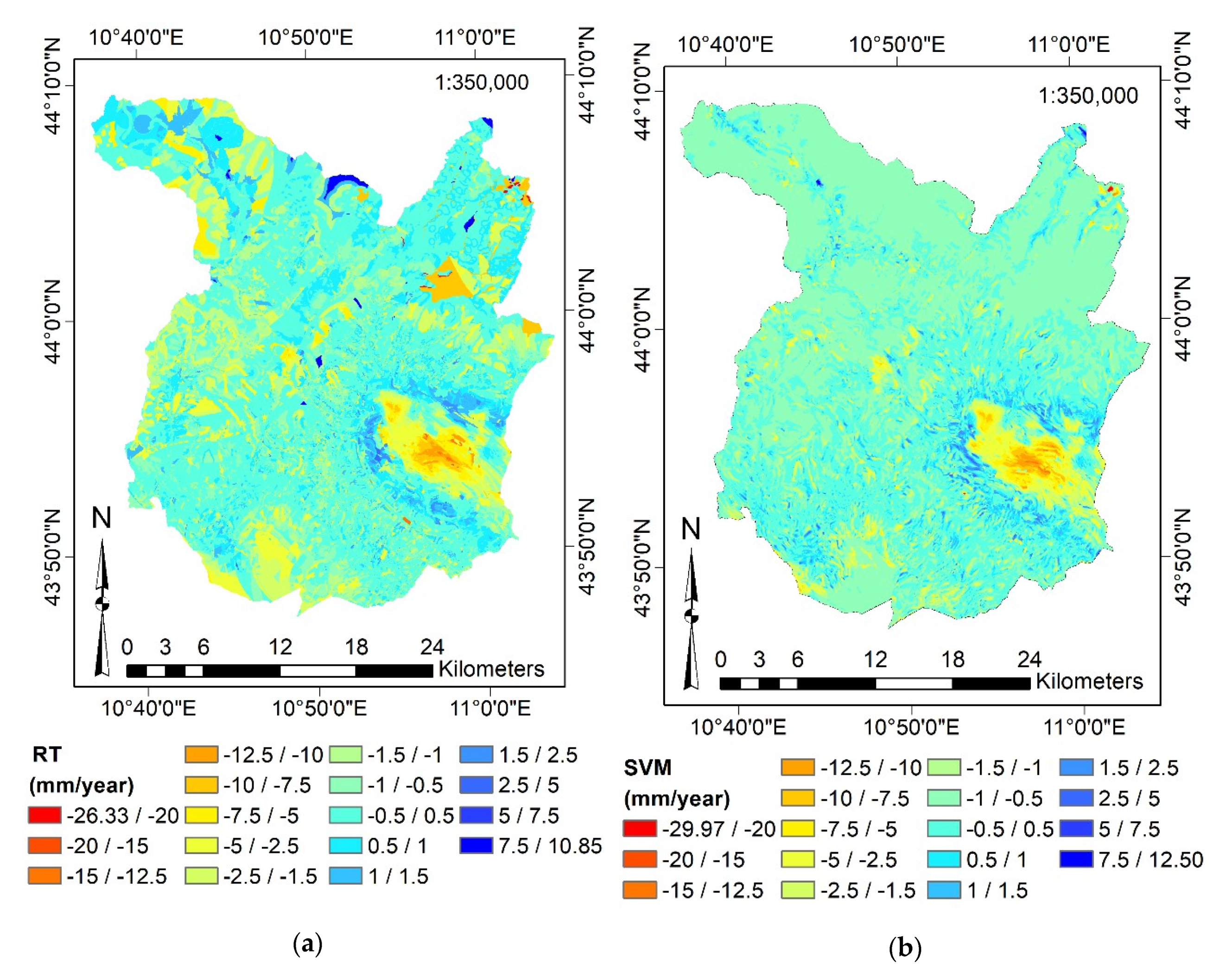
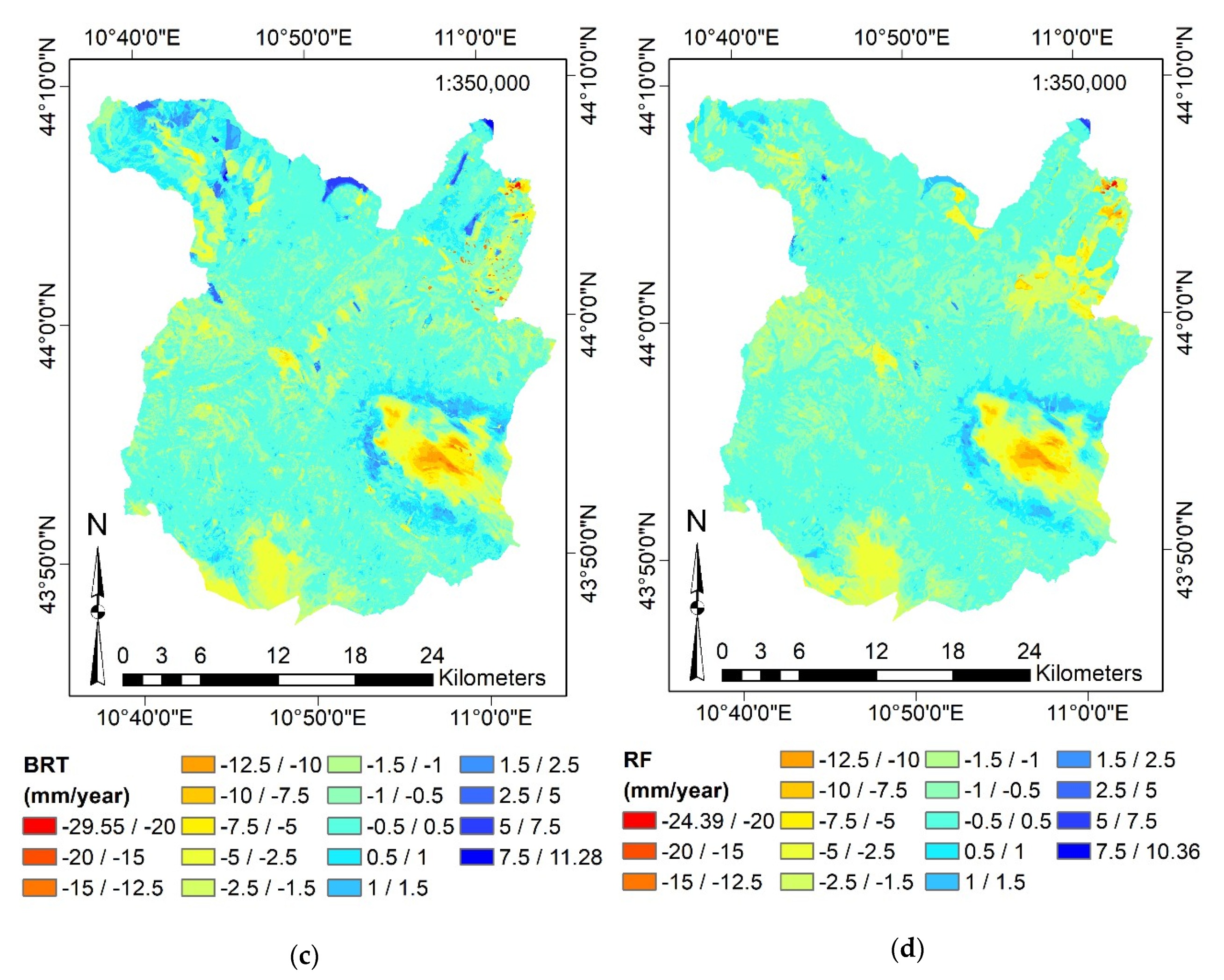
Once the MLAs have been trained and tested, they can be implemented for mapping surface motion over the entire study area. It is worth mentioning that the area is composed of 14,962,725 cells of a size of 10 m × 10 m. Indeed, in order to make predictions by the MLAs, we have collected the same input features for each cell of the study area. Figure 9 reports the predicted surface motion maps for all the MLAs.
Qualitatively speaking, we can note that all the maps are similar, both in shape and in the magnitude of the surface motion predictions. All the maps appropriately detect the subsidence occurring at the city center of Pistoia, and the uplift effect at the boundary of the city. Moreover, a further significant effect of subsidence is expected in the southern part of the province. In this area, there is a shortage of PS so that these maps can be a useful and reliable supporting tool for the managing bodies of the territory and infrastructures. The MLAs probably predict subsidence effects since this area is orographically and hydrologically similar to the area of the city of Pistoia.
Moreover, in decision tree-based algorithms, i.e., RT, BRT, and RF, we can see the effects of predictions made by MLAs implementing piecewise functions. Indeed, there are some areas, even extended ones, where the predicted value of surface motion assumes the same value. This fact is the obvious consequence of the construction process of such algorithms, which involves the clear subdivision into nodes through decision rules learned during the training phase. This effect is strongly visible in the RT algorithm, especially in the extreme north-west area and in some areas north of the city of Pistoia. In the BRT and RF algorithms, being ensemble learners, this fact is lighter, and the issue of prediction using piecewise functions is less marked since they can count on a large number of RT. The SVM algorithm, on the other hand, relying on prediction through the identification of a hyperplane, does not suffer from this issue and can make reliable predictions for the entire study area, even in areas where there was a substantial shortage of PS.
Therefore, we can say that the implemented MLAs are efficient and suitable predictors of surface motion in areas where there were numerous PS. They can adequately highlight both movements due to subsidence effects and uplifts. In areas where there were fewer PS, decision trees-based algorithms are less performing, because they suffer from prediction through piecewise functions. The SVM algorithm appears to be able to make appropriate predictions over the whole study area.

4.5. Predictor Importance

As a final step of the modeling, the PI of the input factors has been computed. This step allows understating which features are the most important in the prediction of surface motion; therefore, it is also possible to identify which features may be more correlated to the phenomenon. Moreover, this step is useful to verify if the wrapper feature approaches performed correctly and, thus, if the most relevant input features have been considered. To carry out the PI computation, a 500-RT-based RF has been trained considering all the 29 collected input features, and the average impurity (i.e., the MSE) decrease has been considered as parameter of importance. Table 6 shows the PI of the MLAs. Moreover, the features elected by wrappers have been highlighted.
The target output is strongly related to the composition of the subsoil, in terms of organic, clay, and silt content. This is consistent with Reference [17], where the authors stated that subsidence effects of the city of Pistoia could be related to the combination of overexploitation of water and soft compaction layers. The composition of subsoil influences the drainage capacity; indeed, such a feature is positioned in the top zone of the ranking as well. Flood susceptibility, distance from landslides, landslide susceptibility, and erosion susceptibility are still in the higher part of the rank. This fact is likely related to the orography of the study area. Indeed, subsidence and uplift are occurring on the plains of the south-west part of the study area, far from the mountainous areas, where the most landslides and erosion phenomena may occur. Moreover, these plain areas are certainly more susceptible to floods than mountainous areas. Therefore, MLAs have probably learned that most of the surface motions occurred over the plain areas, where there is a similar degree of flood susceptibility, distance from landslides, landslide susceptibility, and erosion susceptibility. Accordingly, the algorithms identify such features as more important than others. The earthquake susceptibility (i.e., the probable magnitude of an occurring earthquake) has been found as an important feature. This information is interesting and should deserve further investigations that relate current surface motions and previously occurring earthquakes. It is interesting to observe that also rainfall seems to be an important feature; this could be related to the combination of orography and composition of the subsoil (i.e., for the city of Pistoia, it means plain areas and a high percentage of silt), which leads to strong surface motions. The last mention is linked to the exploitation of water in the area surrounding the city of Pistoia, which resulted in subsidence. This fact can be taken into consideration through the features related to land use or the type of area. Indeed, these two variables have a non-negligible PI.
As for the wrapper approaches, we can note that most of the important features have been considered and that the process should have been carried out correctly. MLAs describe the subsoil composition by Clay and Silt content (in Backward wrapper), while the orography is considered by distance from landslide and elevation. Furthermore, earthquake susceptibility has been considered. Hydrologically, the MLAs can account for rainfall, river density, and distance from rivers. Finally, for what concerns the social system, MLAs consider the type of area. The wrappers did not consider the last twelve variables with the lowest PI. Therefore, it seems that the wrappers have simplified the phenomenon by excluding all the less important features, and also considering the important ones as a non-redundant subset of them (i.e., two features for describing the subsoil composition, two features for describing the topography, three features for describing the hydrology, and one feature for describing the social system).
To confirm what has just been described, Table 7 highlights the performance of MLAs trained with the complete set of input features.
The metrics in Table 7 demonstrate the decrease in performance overlooking the use of feature selection approaches.
Observing, for example, the RF performances, and comparing them with those shown in Table 5, we can recognize a meaningful reduction of all of them. Indeed, the coefficient R2 diminishes both in the training phase (from 0.9828 to 0.9724) and significantly in the test phase (from 0.9466 to 0.8709). The difference in R2 between training and test is higher than that shown by the wrapper-based RF (0.1015 versus 0.0362); this could denote that the RF trained by all the input features is more likely prone to overfit the data. Training an algorithm with more input features (29 versus 9) likely leads to a deeper and more complex model and, accordingly, making predictions on new data is more complicated. Moreover, complex models affect the interpretability. The RMSE and MAE are significantly higher, both in the training and test phase. The prediction accuracy is, therefore, lower.
The same consideration can also be extended to the RT and BRT. Indeed, all the RMSE and MAE values are higher than those shown in Table 5, while R2 values are lower. The SVM trained with all the input features is an inefficient and unreliable model. Its performances shown in Table 7 are dramatically lower than those shown in Table 5. In the framework of this research, SVM could not be used for practical purposes if a feature selection step is neglected.
The use of wrapper approaches for discovering and using as input the most relevant features has been proved crucial to obtain the best models from every perspective (e.g., better interpretability, higher goodness-of-fit, higher predictive performance, and lower risk of overfitting).

4.6. Validation on Stretches of Two-lane Rural Roads

In this part, three significant case studies are reported to verify the reliability of the procedure for road monitoring and inspection activities. Therefore, we would like to judge whether the surface motion mapping allows for the precise identification of any structural deficiencies and damage to road pavements. In order to identify the condition of road pavement structures, the two-lane rural road network graph has been overlayed on the map of surface motions predicted by SVM, assuming that it is the most reliable, suitable, and accurate model among the calibrated MLAs. Figure 10 reports the location of three potentially critical road sites detected by the models, while in Appendix B are reported some images by Google map (https://www.google.com/maps) that depict the past and present condition of road pavements belonging to such sites.
A roundabout represents the first case study (Figure 10a) at the north-west boundary of the city center of Pistoia on the SR435. The same case study has been identified as the most critical road site on SR435 in our previous research [2]. Figure A9 highlights a pavement structure in good condition in 2012, while a notable collapse of the roundabout side has occurred recently (2019).
The second case study (Figure 10b) is located on a road stretch at the south-east boundary of the city center of Pistoia on the SR66 (southern part). From Figure A10, we can appreciate two images of the same road section, about 100 m away from each other. The stretch considered is a straight line, and in 2008 it had a road pavement in good condition. After 11 years, in 2019, it shows severe damage to the pavement. In Figure A10a, we can see how the whole area on the extreme left of the roadway is cracking. Furthermore, in Figure A10b, the same area of the carriageway is undergoing a significant sinking, highlighted by the stagnation of water.
The third case study (Figure 10c) is located in the mountainous northern part of the study area, on a circular curve of the SR66 (northern part). The images proposed in Figure A11 describe the curve in the two directions of travel. Images relating to the acceptable conditions of the pavement in the past (the year 2011) and recent unsatisfactory conditions (the year 2019) are compared. In fact, after about eight years, the pavement shows significant deterioration and depressions in both directions of travel. It appears that a large part of the structure is moving downstream.

4.7. Use of the Procedure by Road Authorities

Road authorities can exploit the proposed procedure in different ways:
  • It allows quantifying the surface motion of road pavements in every point of the infrastructures, even in those areas where there is no presence of PS detected by InSAR techniques; road authorities could use the calibrated MLAs in other areas than where they were trained;
  • The most influential and relevant factors on the deterioration of pavements connected to environmental and social parameters can be quantified. Consequently, road authorities can arrange appropriate and specific maintenance interventions that also consider exogenous factors;
  • Monitoring and inspection activities of complex and extensive networks can be carried out with a sufficient degree of accuracy, a high level of detail, and low cost (once the procedure has been calibrated). Nonetheless, the methodology cannot replace modern Non-Destructive High-Performance Techniques, such as Falling Weight Deflectometer, Ground Penetrating Radar, or Profilometric measurements. However, thanks to the findings suggested by the procedure, road authorities may have a tool for identifying a reduced set of road sites to be inspected. Once specific admissibility thresholds of displacement (both negative and positive) have been set, those road sites that require more attention will be automatically extracted;
  • By this procedure, road authorities may have more objective criteria for the planning of new infrastructures. Indeed, thanks to the surface motion maps, it is possible to identify the areas in which building a new infrastructure may be inappropriate. If admissibility thresholds are set for this activity, different categories of areas could be discovered, such as good, acceptable, not recommended, or prohibited areas for the development of a new infrastructural corridor;
Furthermore, thanks to the Sentinel-1 satellites, every six days, it is possible to have new PS and new measurements of the PS already present in the area. Consequently, it is possible to update the MLAs with the latest measures, having predictive models that are accurate over time.

4.8. Future Works

This paper constitutes an extended, updated, and improved version of our previous work [2]. Nonetheless, the research can be further enhanced and refined through:
  • Extend the study area to different Provinces, up to the mapping of the entire Tuscany Region (23,000 km2), relying on over 830,000 PS;
  • It would be advisable to integrate information relating to the ascending and descending orbit to estimate the surface motion ratio in the vertical direction and not in the Line-Of-Sight direction of the sensor;
  • Consider the entire road network present in the study area (including the urban sections of the two-lane rural roads and other roads not managed by the TRRA);
  • Consider also the railway network, extending the field of use to all the so-called linear infrastructures;
  • Test different feature selection approaches, such as the PCA, and compare the results obtained with the wrapper approaches implemented in this study;
  • Calibration of more complex MLAs, such as Neural Networks (both Multilayer Perceptron and Convolutional Neural Networks), and comparison with the already implemented MLAs. Furthermore, algorithms related to the stacking technique could be developed (i.e., parallel and independent training of various learners and the aggregation of their predictions by another MLA, whose inputs are learners’ predictions).

5. Conclusions

In the present paper, we defined a step-by-step procedure potentially useful for supporting infrastructure monitoring, inspection, and planning activities. Specifically, we discussed the use of PS-InSAR measurements and GIS analyses in combination with Machine Learning Algorithms for modeling and predicting the surface motion ratio caused by environmental factors in terms of mm/year of an area of interest.
In order to achieve this purpose, four different algorithms have been trained, validated, evaluated, and compared for the Province of Pistoia, Tuscany Region, central Italy. We calibrated two single learners, i.e., Regression Tree and Support Vector Machine, and two ensemble learners, i.e., Random Forest and Boosted Regression Trees; such algorithms have been defined for the prediction of the surface motion ratio of each point of a road pavement structure, with a resolution of 10 m. The surface motion ratio is the numerical target output of the models; we accounted for more than 52,000 Persistent Scatterers. The input features of the models are represented by a set of 29 topographical-, hydrological-, environmental-, and social system-based information collected by GIS platforms. Considering the complexity of the phenomenon and the strongly non-linear relations between inputs and output, we tried to implement a modeling strategy that was as automatic as possible, regarding the choice of the most relevant features and the definition of the hyperparameters of the MLAs. Indeed, a backward wrapper feature selection approach identified the subset of most relevant features, reducing the number of predictors from 29 to 9, including Elevation, Rainfall, Distance from rivers, Distance from landslides, Earthquake susceptibility, Type of area, River Density, and Silt and Clay content of the subsoil.
Once the dataset has been randomly split into training (70%) and test (30%) sets, the Machine Learning Algorithms have been trained and validated by a Bayesian Optimization Algorithm and a 10-Fold Cross-Validation. Therefore, we evaluated the performance of such models by R2, RMSE, MAE, Scatterplots, and the Taylor Diagram. The numerical performance parameters highlight that SVM and BRT are the most suitable algorithms, while the use of scatterplots reveals that despite BRT shows satisfactory predictive performance during the test phase, it may suffer from overfitting issues during training. Finally, the Taylor Diagram allows comparing the models by a graph-based visualization. Through this diagram we verified that SVM and BRT are the best algorithms, considering that BRT shows the highest Correlation Coefficient (0.96) and the lowest Root Mean Square Error (0.44 mm/year), while the SVM has the lowest difference between the standard deviation of its predictions (2.05 mm/year) and that of the reference population (2.09 mm/year). In the conclusion of the workflow, we mapped the surface motion over the entire study area and overlayed the road network graph with the SVM predictions. Once the critical road sites have been detected, we proposed three case studies to show the reliability of the suggested procedure.
We would like to advise road authorities to implement a similar approach for supporting efficiently their decision-making processes involving road maintenance interventions, monitoring, inspection activities, and planning of new infrastructural works.

Author Contributions

Conceptualization, N.F., M.M., M.L., and M.G.; methodology, N.F., M.M., M.L., and M.G.; software, N.F.; validation, N.F., M.M., M.L., and M.G.; formal analysis, N.F.; investigation, N.F.; resources, N.F., M.M., P.L., M.L., and M.G.; data curation, N.F.; writing—original draft, N.F.; writing—review and editing, N.F., M.M., P.L., M.L., and M.G.; visualization, N.F.; supervision, M.L. and M.G.; project administration, P.L., M.L., and M.G.; funding acquisition, P.L. All authors have read and agreed to the published version of the manuscript.

Funding

This work was supported by the PRIN (Projects of Relevant National Interest) n°20179BP4SM promoted by the Italian Ministry of Education, University and Research (MIUR).

Acknowledgments

The authors would like to thank the Tuscany Region Administration for providing information related to the study area.

Conflicts of Interest

The authors declare no conflict of interest.

Appendix A

Figure A1. Land use map.
Remotesensing 12 03976 g0a1
Figure A2. Information collected: (a) Type of Area (Urban or Rural according to the Italian Road Design standards [ref]); (b) rain gauge stations; (c) earthquakes occurred; (d) landslides occurred.
Remotesensing 12 03976 g0a2
Figure A3. Information collected—susceptibilities: (a) Landslide susceptibility; (b) Erosion susceptibility; (c) Flood susceptibility; (d) Drainage capacity of the subsoil.
Remotesensing 12 03976 g0a3
Figure A4. Information collected—subsoil composition: (a) Sand content (%); (b) Silt content (%); (c) Clay content (%); (d) Organic content (%).
Remotesensing 12 03976 g0a4
Figure A5. Input features—topographical-based computed factors: (a) Slope; (b) Aspect; (c) CI; (d) Curvature; (e) VRM; (f) TPI; (g) TRI; (h) SL.
Remotesensing 12 03976 g0a5aRemotesensing 12 03976 g0a5b
Figure A6. Input features—hydrological-based computed factors: (a) SPI; (b) TWI; (c) River density; (d) Rainfall.
Remotesensing 12 03976 g0a6
Figure A7. Input features—environmental-based computed factors: (a) Direct Yearly Solar Radiation; (b) Diffusive Yearly Solar Radiation; (c) WE; (d) Earthquake susceptibility.
Remotesensing 12 03976 g0a7
Figure A8. Input features—Euclidean distances: (a) Distance from rivers; (b) Distance from Landslides.
Remotesensing 12 03976 g0a8
Figure A9. 1st Case study, Road SR435: (a) in 2012; (b) in 2019.
Remotesensing 12 03976 g0a9aRemotesensing 12 03976 g0a9b
Figure A10. 2nd Case study, Road SR66_Sud: (a) in 2008, (b) in 2019.
Remotesensing 12 03976 g0a10aRemotesensing 12 03976 g0a10b
Figure A11. 3rd Case study, Road SR66_Nord: (a) in 2011; (b) in 2019.
Remotesensing 12 03976 g0a11aRemotesensing 12 03976 g0a11b

References

  1. Maboudi, M.; Amini, J.; Hahn, M.; Saati, M. Object-based road extraction from satellite images using ant colony optimization. Int. J. Remote Sens. 2017, 38, 179–198. [Google Scholar] [CrossRef]
  2. Fiorentini, N.; Maboudi, M.; Losa, M.; Gerke, M. Assessing Resilience of Infrastructures Towards Exogenous Events by Using PS-InSAR-Based Surface Motion Estimates and Machine Learning Regression Techniques. ISPRS Ann. Photogramm. Remote Sens. Spat. Inf. Sci. 2020, 4, 19–26. [Google Scholar] [CrossRef]
  3. Ouchi, K. Recent Trend and Advance of Synthetic Aperture Radar with Selected Topics. Remote Sens. 2013, 5, 716–807. [Google Scholar] [CrossRef] [Green Version]
  4. Graham, L.C. Synthetic Interferometer Radar For Topographic Mapping. Proc. IEEE 1974. [Google Scholar] [CrossRef]
  5. Costantini, M.; Ferretti, A.; Minati, F.; Falco, S.; Trillo, F.; Colombo, D.; Novali, F.; Malvarosa, F.; Mammone, C.; Vecchioli, F.; et al. Analysis of surface deformations over the whole Italian territory by interferometric processing of ERS, Envisat and COSMO-SkyMed radar data. Remote Sens. Environ. 2017, 202, 250–275. [Google Scholar] [CrossRef]
  6. Ferretti, A.; Prati, C.; Rocca, F. Permanent Scatterers in SAR Interferometry. IEEE Trans. Geosci. Remote Sens. 2001, 39, 8–20. [Google Scholar] [CrossRef]
  7. Ferretti, A.; Prati, C.; Rocca, F. Nonlinear Subsidence Rate Estimation Using Permanent Scatterers in Differential SAR Interferometry. IEEE Trans. Geosci. Remote Sens. 2000, 38, 2202–2212. [Google Scholar] [CrossRef] [Green Version]
  8. Ferretti, A.; Monti-Guarnieri, A.; Prati, C.; Rocca, F. InSAR Principles: Guidelines for SAR Interferometry Processing and Interpretation; TM-19; ESA Publications: Auckland, New Zealand, 2007. [Google Scholar]
  9. Gheorghe, M.; Armaş, I. Comparison of Multi-Temporal Differential Interferometry Techniques Applied to the Measurement of Bucharest City Subsidence. Procedia Environ. Sci. 2016, 32, 221–229. [Google Scholar] [CrossRef] [Green Version]
  10. Milczarek, W.; Blachowski, J.; Grzempowski, P. Application of Psinsar For Assessment of Surface Deformations in Post-Mining Area-Case Study of the Former Walbrzych Hard Coal Basin (Sw Poland). Acta Geodyn. Geomater. 2017, 14, 41–52. [Google Scholar] [CrossRef]
  11. Samsonov, S.; d’Oreye, N.; Smets, B. Ground deformation associated with post-mining activity at the French-German border revealed by novel InSAR time series method. Int. J. Appl. Earth Obs. Geoinf. 2013. [Google Scholar] [CrossRef]
  12. Perissin, D.; Wang, Z.; Lin, H. Shanghai subway tunnels and highways monitoring through Cosmo-SkyMed Persistent Scatterers. ISPRS J. Photogramm. Remote Sens. 2012, 73, 58–67. [Google Scholar] [CrossRef]
  13. Wang, H.; Feng, G.; Xu, B.; Yu, Y.; Li, Z.; Du, Y.; Zhu, J. Deriving spatio-temporal development of ground subsidence due to subway construction and operation in Delta regions with PS-InSAR data: A case study in Guangzhou, China. Remote Sens. 2017, 9, 1004. [Google Scholar] [CrossRef] [Green Version]
  14. Xavier, D.; Declercq, P.-Y.; Bruno, F.; Jérôme, B.; Albert, T.; Julien, V. Uplift Revealed by Radar Interferometry Around Liege (Belgium): A Relation with Rising Mining Groundwater. Post Mining 2008, 6–8. [Google Scholar]
  15. Solari, L.; Del Soldato, M.; Bianchini, S.; Ciampalini, A.; Ezquerro, P.; Montalti, R.; Raspini, F.; Moretti, S. From ERS 1/2 to Sentinel-1: Subsidence Monitoring in Italy in the Last Two Decades. Front. Earth Sci. 2018, 6, 149. [Google Scholar] [CrossRef]
  16. Rosi, A.; Tofani, V.; Agostini, A.; Tanteri, L.; Tacconi Stefanelli, C.; Catani, F.; Casagli, N. Subsidence mapping at regional scale using persistent scatters interferometry (PSI): The case of Tuscany region (Italy). Int. J. Appl. Earth Obs. Geoinf. 2016, 52, 328–337. [Google Scholar] [CrossRef]
  17. Del Soldato, M.; Farolfi, G.; Rosi, A.; Raspini, F.; Casagli, N. Subsidence Evolution of the Firenze–Prato–Pistoia Plain (Central Italy) Combining PSI and GNSS Data. Remote Sens. 2018, 10, 1146. [Google Scholar] [CrossRef] [Green Version]
  18. Benattou, M.M.; Balz, T.; Minsheng, L. Measuring Surface Subsidence in Wuhan, China with Sentinel-1 Data Using Psinsar. In Proceedings of the 2018 ISPRS TC III Mid-term Symposium Developments, Technologies and Applications in Remote Sensing, Beijing, China, 7–10 May 2018. [Google Scholar] [CrossRef] [Green Version]
  19. Ng, A.H.-M.; Ge, L.; Li, X.; Abidin, H.Z.; Andreas, H.; Zhang, K. Mapping land subsidence in Jakarta, Indonesia using persistent scatterer interferometry (PSI) technique with ALOS PALSAR. Int. J. Appl. Earth Obs. Geoinf. 2012, 18, 232–242. [Google Scholar] [CrossRef]
  20. Comerci, V.; Vittori, E.; Cipolloni, C.; Di Manna, P.; Guerrieri, L.; Nisio, S.; Succhiarelli, C.; Ciuffreda, M.; Bertoletti, E. Geohazards Monitoring in Roma from InSAR and In Situ Data: Outcomes of the PanGeo Project. Pure Appl. Geophys. 2015. [Google Scholar] [CrossRef]
  21. Bianchini, S.; Pratesi, F.; Nolesini, T.; Casagli, N. Building Deformation Assessment by Means of Persistent Scatterer Interferometry Analysis on a Landslide-Affected Area: The Volterra (Italy) Case Study. Remote Sens. 2015, 7, 4678–4701. [Google Scholar] [CrossRef] [Green Version]
  22. Wasowski, J.; Bovenga, F. Investigating landslides and unstable slopes with satellite Multi Temporal Interferometry: Current issues and future perspectives. Eng. Geol. 2014, 174, 103–138. [Google Scholar] [CrossRef]
  23. Rosi, A.; Tofani, V.; Tanteri, L.; Tacconi Stefanelli, C.; Agostini, A.; Catani, F.; Casagli, N. The new landslide inventory of Tuscany (Italy) updated with PS-InSAR: Geomorphological features and landslide distribution. Landslides 2018. [Google Scholar] [CrossRef] [Green Version]
  24. Yin, Y.; Zheng, W.; Liu, Y.; Zhang, J.; Li, X. Integration of GPS with InSAR to monitoring of the Jiaju landslide in Sichuan, China. Landslides 2010. [Google Scholar] [CrossRef]
  25. Schlögel, R.; Doubre, C.; Malet, J.P.; Masson, F. Landslide deformation monitoring with ALOS/PALSAR imagery: A D-InSAR geomorphological interpretation method. Geomorphology 2015, 231, 314–330. [Google Scholar] [CrossRef]
  26. Béjar-Pizarro, M.; Notti, D.; Mateos, R.M.; Ezquerro, P.; Centolanza, G.; Herrera, G.; Bru, G.; Sanabria, M.; Solari, L.; Duro, J.; et al. Mapping vulnerable urban areas affected by slow-moving landslides using Sentinel-1InSAR data. Remote Sens. 2017, 9, 876. [Google Scholar] [CrossRef] [Green Version]
  27. Riedel, B.; Walther, A. InSAR processing for the recognition of landslides. Adv. Geosci. 2008. [Google Scholar] [CrossRef] [Green Version]
  28. Hoppe, E.; Bruckno, B.; Campbell, E.; Acton, S.; Vaccari, A.; Stuecheli, M.; Bohane, A.; Falorni, G.; Morgan, J. Transportation Infrastructure Monitoring Using Satellite Remote Sensing. In Materials and Infrastructures 1; John Wiley & Sons, Inc.: Hoboken, NJ, USA, 2016; pp. 185–198. [Google Scholar]
  29. Galve, J.P.; Castañeda, C.; Gutiérrez, F. Railway deformation detected by DInSAR over active sinkholes in the Ebro Valley evaporite karst, Spain. Hazards Earth Syst. Sci. 2015, 15, 2439–2448. [Google Scholar] [CrossRef] [Green Version]
  30. Galve, J.P.; Castañeda, C.; Gutiérrez, F.; Herrera, G. Assessing sinkhole activity in the Ebro Valley mantled evaporite karst using advanced DInSAR. Geomorphology 2015, 229, 30–44. [Google Scholar] [CrossRef] [Green Version]
  31. Ferentinou, M.; Witkowski, W.; Hejmanowski, R.; Grobler, H.; Malinowska, A. Detection of sinkhole occurrence, experiences from South Africa. Proc. Int. Assoc. Hydrol. Sci. 2020, 382, 77–82. [Google Scholar] [CrossRef] [Green Version]
  32. Villarroel, C.D.; Beliveau, G.T.; Forte, A.P.; Monserrat, O.; Morvillo, M. DInSAR for a regional inventory of active rock glaciers in the Dry Andes Mountains of Argentina and Chile with sentinel-1 data. Remote Sens. 2018, 10, 1588. [Google Scholar] [CrossRef] [Green Version]
  33. Nagler, T.; Mayer, C.; Rott, H. Feasibility of DINSAR for mapping complex motion fields of alpine ice- and rock-glaciers. In Proceedings of the Third International Symposium on Retrieval of Bio- and Geophysical Parameters from SAR Data for Land Applications, Sheffield, UK, 11–14 September 2001. [Google Scholar]
  34. Reinosch, E.; Buckel, J.; Dong, J.; Gerke, M.; Baade, J.; Riedel, B. InSAR time series analysis of seasonal surface displacement dynamics on the Tibetan Plateau. Cryosph. 2020, 14, 1633–1650. [Google Scholar] [CrossRef]
  35. Solari, L.; Ciampalini, A.; Raspini, F.; Bianchini, S.; Moretti, S. PSInSAR analysis in the pisa urban area (Italy): A case study of subsidence related to stratigraphical factors and urbanization. Remote Sens. 2016, 8, 120. [Google Scholar] [CrossRef] [Green Version]
  36. Balz, T.; Düring, R. Infrastructure stability surveillance with high resolution InSAR. Proc. IOP Conf. Ser. Earth Environ. Sci. 2017, 57, 12013. [Google Scholar] [CrossRef]
  37. Xing, X.; Chang, H.-C.; Chen, L.; Zhang, J.; Yuan, Z.; Shi, Z.; Xing, X.; Chang, H.-C.; Chen, L.; Zhang, J.; et al. Radar Interferometry Time Series to Investigate Deformation of Soft Clay Subgrade Settlement—A Case Study of Lungui Highway, China. Remote Sens. 2019, 11, 429. [Google Scholar] [CrossRef] [Green Version]
  38. Bakon, M.; Perissin, D.; Lazecky, M.; Papco, J. Infrastructure Non-linear Deformation Monitoring Via Satellite Radar Interferometry. Procedia Technol. 2014, 16, 294–300. [Google Scholar] [CrossRef] [Green Version]
  39. D’Aranno, P.; Di Benedetto, A.; Fiani, M.; Marsella, M. Remote Sensing Technologies for Linear Infrastructure Monitoring. ISPRS Int. Arch. Photogramm. Remote Sens. Spat. Inf. Sci. 2019, XLII-2/W11, 461–468. [Google Scholar] [CrossRef] [Green Version]
  40. Murdzek, R.; Malik, H.; Leśniak, A. The use of the DInSAR method in the monitoring of road damage caused by mining activities. In E3S Web of Conferences; EDP Sciences: Les Ulis, France, 2018; p. 02005. [Google Scholar] [CrossRef] [Green Version]
  41. Wasowski, J.; Bovenga, F.; Nutricato, R.; Nitti, D.O.; Chiaradia, M.T. High resolution satellite multi-temporal interferometry for monitoring infrastructure instability hazards. Innov. Infrastruct. Solut. 2017, 2, 27. [Google Scholar] [CrossRef]
  42. Karimzadeh, S.; Matsuoka, M. Remote Sensing X-Band SAR Data for Land Subsidence and Pavement Monitoring. Sensors 2020, 20, 4751. [Google Scholar] [CrossRef]
  43. Peduto, D.; Huber, M.; Speranza, G.; van Ruijven, J.; Cascini, L. DInSAR data assimilation for settlement prediction: Case study of a railway embankment in the Netherlands. Can. Geotech. J. 2017, 54, 502–517. [Google Scholar] [CrossRef] [Green Version]
  44. Rao, X.; Tang, Y. Small baseline subsets approach of DInSAR for investigating land surface deformation along the high-speed railway. In Land Surface Remote Sensing II; Elsevier: Amsterdam, The Netherlands, 2014. [Google Scholar]
  45. Li, T.; Hong, Z.; Chao, W.; Yixian, T. Comparison of Beijing-Tianjin Intercity Railway deformation monitoring results between ASAR and PALSAR data. In Proceedings of the International Geoscience and Remote Sensing Symposium (IGARSS), Honolulu, HI, USA, 25–30 July 2010. [Google Scholar]
  46. Poreh, D.; Iodice, A.; Riccio, D.; Ruello, G. Railways’ stability observed in Campania (Italy) by InSAR data. Eur. J. Remote Sens. 2016. [Google Scholar] [CrossRef] [Green Version]
  47. Sousa, J.J.; Bastos, L. Multi-temporal SAR interferometry reveals acceleration of bridge sinking before collapse. Nat. Hazards Earth Syst. Sci. 2013. [Google Scholar] [CrossRef]
  48. Qin, X.; Ding, X.; Liao, M.; Zhang, L.; Wang, C. A bridge-tailored multi-temporal DInSAR approach for remote exploration of deformation characteristics and mechanisms of complexly structured bridges. ISPRS J. Photogramm. Remote Sens. 2019, 156, 27–50. [Google Scholar] [CrossRef]
  49. Fornaro, G.; Reale, D.; Verde, S. Bridge thermal dilation monitoring with millimeter sensitivity via multidimensional SAR imaging. IEEE Geosci. Remote Sens. Lett. 2013. [Google Scholar] [CrossRef]
  50. Peduto, D.; Elia, F.; Montuori, R. Probabilistic analysis of settlement-induced damage to bridges in the city of Amsterdam (The Netherlands). Transp. Geotech. 2018, 14, 169–182. [Google Scholar] [CrossRef]
  51. Sousa, J.M.M.; Lazecky, M.; Hlavacova, I.; Bakon, M.; Patrício, G.; Perissin, D. Satellite SAR Interferometry for Monitoring Dam Deformations in Portugal. In Proceedings of the Second International Dam World Conference, Lisbon, Portugal, 21–24 April 2015; pp. 21–24. [Google Scholar]
  52. Mura, J.C.; Gama, F.F.; Paradella, W.R.; Negrão, P.; Carneiro, S.; de Oliveira, C.G.; Brandão, W.S. Monitoring the vulnerability of the dam and dikes in Germano iron mining area after the collapse of the tailings dam of fundão (Mariana-MG, Brazil) using DInSAR techniques with terraSAR-X data. Remote Sens. 2018, 10, 1507. [Google Scholar] [CrossRef] [Green Version]
  53. Tomás, R.; Cano, M.; García-Barba, J.; Vicente, F.; Herrera, G.; Lopez-Sanchez, J.M.; Mallorquí, J.J. Monitoring an earthfill dam using differential SAR interferometry: La Pedrera dam, Alicante, Spain. Eng. Geol. 2013, 157, 21–32. [Google Scholar] [CrossRef]
  54. Di Martire, D.; Iglesias, R.; Monells, D.; Centolanza, G.; Sica, S.; Ramondini, M.; Pagano, L.; Mallorquí, J.J.; Calcaterra, D. Comparison between Differential SAR interferometry and ground measurements data in the displacement monitoring of the earth-dam of Conza della Campania (Italy). Remote Sens. Environ. 2014, 148, 58–69. [Google Scholar] [CrossRef]
  55. Ozden, A.; Faghri, A.; Li, M.; Tabrizi, K. Evaluation of Synthetic Aperture Radar Satellite Remote Sensing for Pavement and Infrastructure Monitoring. Procedia Eng. 2016, 145, 752–759. [Google Scholar] [CrossRef] [Green Version]
  56. Deng, Z.; Ke, Y.; Gong, H.; Li, X.; Li, Z. Land subsidence prediction in Beijing based on PS-InSAR technique and improved Grey-Markov model Land subsidence prediction in Beijing based on PS-InSAR technique and improved Grey-Markov model. GIScience Remote Sens. 2017, 54, 797–818. [Google Scholar] [CrossRef]
  57. Tien Bui, D.; Tuan, T.A.; Klempe, H.; Pradhan, B.; Revhaug, I. Spatial prediction models for shallow landslide hazards: A comparative assessment of the efficacy of support vector machines, artificial neural networks, kernel logistic regression, and logistic model tree. Landslides 2016, 13, 361–378. [Google Scholar] [CrossRef]
  58. Xie, Z.; Chen, G.; Meng, X.; Zhang, Y.; Qiao, L.; Tan, L. A comparative study of landslide susceptibility mapping using weight of evidence, logistic regression and support vector machine and evaluated by SBAS-InSAR monitoring: Zhouqu to Wudu segment in Bailong River Basin, China. Environ. Earth Sci. 2017, 76, 313. [Google Scholar] [CrossRef]
  59. Al-Najjar, H.A.H.; Kalantar, B.; Pradhan, B.; Saeidi, V. Conditioning factor determination for mapping and prediction of landslide susceptibility using machine learning algorithms. In Earth Resources and Environmental Remote Sensing/GIS; Applications, X., Schulz, K., Nikolakopoulos, K.G., Michel, U., Eds.; SPIE: Washington, DC, USA, 2019; Volume 11156, p. 19. [Google Scholar]
  60. Dou, J.; Yunus, A.P.; Tien Bui, D.; Merghadi, A.; Sahana, M.; Zhu, Z.; Chen, C.-W.; Khosravi, K.; Yang, Y.; Pham, B.T. Assessment of advanced random forest and decision tree algorithms for modeling rainfall-induced landslide susceptibility in the Izu-Oshima Volcanic Island, Japan. Sci. Total Environ. 2019, 662, 332–346. [Google Scholar] [CrossRef] [PubMed]
  61. Hong, H.; Pradhan, B.; Bui, T.; Xu, C.; Youssef, A.M.; Chen, W. Comparison of four kernel functions used in support vector machines for landslide susceptibility mapping: A case study at Suichuan area (China). Geomat. Nat. Hazards Risk 2017, 8, 544–569. [Google Scholar] [CrossRef]
  62. Yeon, Y.-K.; Han, J.-G.; Ryu, K.H. Landslide susceptibility mapping in Injae, Korea, using a decision tree. Eng. Geol. 2010, 116, 274–283. [Google Scholar] [CrossRef]
  63. Devkota, K.C.; Regmi, A.D.; Pourghasemi, H.R.; Yoshida, K.; Pradhan, B.; Ryu, I.C.; Dhital, M.R.; Althuwaynee, O.F. Landslide susceptibility mapping using certainty factor, index of entropy and logistic regression models in GIS and their comparison at Mugling–Narayanghat road section in Nepal Himalaya. Nat. Hazards 2013, 65, 135–165. [Google Scholar] [CrossRef]
  64. Pradhan, B.; Lee, S. Landslide susceptibility assessment and factor effect analysis: Backpropagation artificial neural networks and their comparison with frequency ratio and bivariate logistic regression modelling. Environ. Model. Softw. 2010, 25, 747–759. [Google Scholar] [CrossRef]
  65. Polykretis, C.; Ferentinou, M.; Chalkias, C. A comparative study of landslide susceptibility mapping using landslide susceptibility index and artificial neural networks in the Krios River and Krathis River catchments (northern Peloponnesus, Greece). Bull. Eng. Geol. Environ. 2015, 74, 27–45. [Google Scholar] [CrossRef]
  66. Kalantar, B.; Pradhan, B.; Naghibi, S.A.; Motevalli, A.; Mansor, S. Assessment of the effects of training data selection on the landslide susceptibility mapping: A comparison between support vector machine (SVM), logistic regression (LR) and artificial neural networks (ANN) Assessment of the effects of training data selec. Geomat. Nat. Hazards Risk 2017. [Google Scholar] [CrossRef]
  67. Marjanović, M.; Kovačević, M.; Bajat, B.; Voženílek, V. Landslide susceptibility assessment using SVM machine learning algorithm. Eng. Geol. 2011, 123, 225–234. [Google Scholar] [CrossRef]
  68. Nefeslioglu, H.A.; Sezer, E.; Gokceoglu, C.; Bozkir, A.S.; Duman, T.Y. Assessment of Landslide Susceptibility by Decision Trees in the Metropolitan Area of Istanbul, Turkey. Math. Probl. Eng. 2010, 2010. [Google Scholar] [CrossRef] [Green Version]
  69. Tien Bui, D.; Shahabi, H.; Omidvar, E.; Shirzadi, A.; Geertsema, M.; Clague, J.; Khosravi, K.; Pradhan, B.; Pham, B.; Chapi, K.; et al. Shallow Landslide Prediction Using a Novel Hybrid Functional Machine Learning Algorithm. Remote Sens. 2019, 11, 931. [Google Scholar] [CrossRef] [Green Version]
  70. Pourghasemi, H.R.; Jirandeh, A.G.; Pradhan, B.; Xu, C.; Gokceoglu, C. Landslide susceptibility mapping using support vector machine and GIS at the Golestan Province, Iran. J. Earth Syst. Sci. 2013, 122, 349–369. [Google Scholar] [CrossRef] [Green Version]
  71. Lee, S.; Pradhan, B. Landslide hazard mapping at Selangor, Malaysia using frequency ratio and logistic regression models. Landslides 2007, 4, 33–41. [Google Scholar] [CrossRef]
  72. Tien Bui, D.; Pradhan, B.; Lofman, O.; Revhaug, I. Landslide Susceptibility Assessment in Vietnam Using Support Vector Machines, Decision Tree, and Naïve Bayes Models. Math. Probl. Eng. 2012, 2012, 1–26. [Google Scholar] [CrossRef] [Green Version]
  73. Pradhan, B. A comparative study on the predictive ability of the decision tree, support vector machine and neuro-fuzzy models in landslide susceptibility mapping using GIS. Comput. Geosci. 2013, 51, 350–365. [Google Scholar] [CrossRef]
  74. Khan, H.; Shafique, M.; Khan, M.A.; Bacha, M.A.; Shah, S.U.; Calligaris, C. Landslide susceptibility assessment using Frequency Ratio, a case study of northern Pakistan. Egypt. J. Remote Sens. Space Sci. 2019, 22, 11–24. [Google Scholar] [CrossRef]
  75. Youssef, A.M.; Pourghasemi, H.R.; Pourtaghi, Z.S.; Al-Katheeri, M.M. Landslide susceptibility mapping using random forest, boosted regression tree, classification and regression tree, and general linear models and comparison of their performance at Wadi Tayyah Basin, Asir Region, Saudi Arabia. Landslides 2016. [Google Scholar] [CrossRef]
  76. Nhu, V.-H.; Mohammadi, A.; Shahabi, H.; Ahmad, B.; Al-Ansari, N.; Shirzadi, A.; Geertsema, M.; Kress, V.R.; Karimzadeh, S.; Valizadeh Kamran, K.; et al. Landslide Detection and Susceptibility Modeling on Cameron Highlands (Malaysia): A Comparison between Random Forest, Logistic Regression and Logistic Model Tree Algorithms. Forests 2020, 11, 830. [Google Scholar] [CrossRef]
  77. Nhu, V.-H.; Zandi, D.; Shahabi, H.; Chapi, K.; Shirzadi, A.; Al-Ansari, N.; Singh, S.K.; Dou, J.; Nguyen, H. Comparison of Support Vector Machine, Bayesian Logistic Regression, and Alternating Decision Tree Algorithms for Shallow Landslide Susceptibility Mapping along a Mountainous Road in the West of Iran. Appl. Sci. 2020, 10, 5047. [Google Scholar] [CrossRef]
  78. Nhu, V.-H.; Shirzadi, A.; Shahabi, H.; Singh, S.K.; Al-Ansari, N.; Clague, J.J.; Jaafari, A.; Chen, W.; Miraki, S.; Dou, J.; et al. Shallow Landslide Susceptibility Mapping: A Comparison between Logistic Model Tree, Logistic Regression, Naïve Bayes Tree, Artificial Neural Network, and Support Vector Machine Algorithms. Int. J. Environ. Res. Public Health 2020, 17, 2749. [Google Scholar] [CrossRef]
  79. Pourghasemi, H.R.; Teimoori Yansari, Z.; Panagos, P.; Pradhan, B. Analysis and evaluation of landslide susceptibility: A review on articles published during 2005–2016 (periods of 2005–2012 and 2013–2016). Arab. J. Geosci. 2018, 11, 193. [Google Scholar] [CrossRef]
  80. Emami, S.N.; Yousefi, S.; Pourghasemi, H.R.; Tavangar, S.; Santosh, M. A comparative study on machine learning modeling for mass movement susceptibility mapping (a case study of Iran). Bull. Eng. Geol. Environ. 2020. [Google Scholar] [CrossRef]
  81. Greco, R.; Sorriso-Valvo, M.; Catalano, E. Logistic Regression analysis in the evaluation of mass movements susceptibility: The Aspromonte case study, Calabria, Italy. Eng. Geol. 2007. [Google Scholar] [CrossRef]
  82. Ferentinou, M.; Chalkias, C. Mapping mass movement susceptibility across greece with gis, ann and statistical methods. In Landslide Science and Practice; Margiottini, C., Canuti, P., Sassa, K., Eds.; Springer: Berlin/Heidelberg, Germany, 2013; pp. 321–327. ISBN 9783642313240. [Google Scholar]
  83. Gayen, A.; Pourghasemi, H.R.; Saha, S.; Keesstra, S.; Bai, S. Gully erosion susceptibility assessment and management of hazard-prone areas in India using different machine learning algorithms. Sci. Total Environ. 2019, 668, 124–138. [Google Scholar] [CrossRef] [PubMed]
  84. Arabameri, A.; Pradhan, B.; Pourghasemi, H.R.; Rezaei, K.; Kerle, N. Spatial Modelling of Gully Erosion Using GIS and R Programing: A Comparison among Three Data Mining Algorithms. Appl. Sci. 2018, 8, 1369. [Google Scholar] [CrossRef] [Green Version]
  85. Arabameri, A.; Pradhan, B.; Rezaei, K. Gully erosion zonation mapping using integrated geographically weighted regression with certainty factor and random forest models in GIS. J. Environ. Manag. 2019, 232, 928–942. [Google Scholar] [CrossRef]
  86. Khosravi, K.; Shahabi, H.; Pham, B.T.; Adamowski, J.; Shirzadi, A.; Pradhan, B.; Dou, J.; Ly, H.-B.; Gróf, G.; Ho, H.L.; et al. A comparative assessment of flood susceptibility modeling using Multi-Criteria Decision-Making Analysis and Machine Learning Methods. J. Hydrol. 2019, 573, 311–323. [Google Scholar] [CrossRef]
  87. Tehrany, M.S.; Pradhan, B.; Jebur, M.N. Flood susceptibility mapping using a novel ensemble weights-of-evidence and support vector machine models in GIS. J. Hydrol. 2014, 512, 332–343. [Google Scholar] [CrossRef]
  88. Tehrany, M.S.; Pradhan, B.; Mansor, S.; Ahmad, N. Flood susceptibility assessment using GIS-based support vector machine model with different kernel types. CATENA 2015, 125, 91–101. [Google Scholar] [CrossRef]
  89. Tien Bui, D.; Khosravi, K.; Shahabi, H.; Daggupati, P.; Adamowski, J.F.; Melesse, A.M.; Thai Pham, B.; Pourghasemi, H.R.; Mahmoudi, M.; Bahrami, S.; et al. Flood Spatial Modeling in Northern Iran Using Remote Sensing and GIS: A Comparison between Evidential Belief Functions and Its Ensemble with a Multivariate Logistic Regression Model. Remote Sens. 2019, 11, 1589. [Google Scholar] [CrossRef] [Green Version]
  90. Pourghasemi, H.R.; Sadhasivam, N.; Yousefi, S.; Tavangar, S.; Ghaffari Nazarlou, H.; Santosh, M. Using machine learning algorithms to map the groundwater recharge potential zones. J. Environ. Manag. 2020. [Google Scholar] [CrossRef]
  91. Naghibi, S.A.; Pourghasemi, H.R. A comparative assessment between three machine learning models and their performance comparison by bivariate and multivariate statistical methods in groundwater potential mapping. Water Resour. Manag. 2015. [Google Scholar] [CrossRef]
  92. Naghibi, S.A.; Pourghasemi, H.R.; Dixon, B. GIS-based groundwater potential mapping using boosted regression tree, classification and regression tree, and random forest machine learning models in Iran. Environ. Monit. Assess. 2016. [Google Scholar] [CrossRef]
  93. Lee, S.; Hyun, Y.; Lee, S.; Lee, M.J. Groundwater potential mapping using remote sensing and GIS-based machine learning techniques. Remote Sens. 2020, 12, 1200. [Google Scholar] [CrossRef] [Green Version]
  94. Rahmati, O.; Yousefi, S.; Kalantari, Z.; Uuemaa, E.; Teimurian, T.; Keesstra, S.; Pham, T.; Tien Bui, D. Multi-Hazard Exposure Mapping Using Machine Learning Techniques: A Case Study from Iran. Remote Sens. 2019, 11, 1943. [Google Scholar] [CrossRef] [Green Version]
  95. Rahmati, O.; Falah, F.; Naghibi, S.A.; Biggs, T.; Soltani, M.; Deo, R.C.; Cerdà, A.; Mohammadi, F.; Tien Bui, D. Land subsidence modelling using tree-based machine learning algorithms. Sci. Total Environ. 2019, 672, 239–252. [Google Scholar] [CrossRef] [PubMed]
  96. Ocak, I.; Seker, S.E. Calculation of surface settlements caused by EPBM tunneling using artificial neural network, SVM, and Gaussian processes. Environ. Earth Sci. 2013, 70, 1263–1276. [Google Scholar] [CrossRef]
  97. Samui, P. Slope stability analysis: A support vector machine approach. Environ. Geol. 2008, 56, 255–267. [Google Scholar] [CrossRef]
  98. Bui, D.T.; Moayedi, H.; Gör, M.; Jaafari, A.; Foong, L.K. Predicting Slope Stability Failure through Machine Learning Paradigms. ISPRS Int. J. Geo-Inf. 2019, 8, 395. [Google Scholar] [CrossRef] [Green Version]
  99. Nguyen, M.D.; Pham, B.T.; Tuyen, T.T.; Hai Yen, H.P.; Prakash, I.; Vu, T.T.; Chapi, K.; Shirzadi, A.; Shahabi, H.; Dou, J.; et al. Development of an Artificial Intelligence Approach for Prediction of Consolidation Coefficient of Soft Soil: A Sensitivity Analysis. Open Constr. Build. Technol. J. 2019, 13, 178–188. [Google Scholar] [CrossRef]
  100. Radhika, Y.; Shashi, M. Atmospheric Temperature Prediction using Support Vector Machines. Int. J. Comput. Theory Eng. 2009, 55–58. [Google Scholar] [CrossRef] [Green Version]
  101. Rahmati, O.; Choubin, B.; Fathabadi, A.; Coulon, F.; Soltani, E.; Shahabi, H.; Mollaefar, E.; Tiefenbacher, J.; Cipullo, S.; Ahmad, B.B.; et al. Predicting uncertainty of machine learning models for modelling nitrate pollution of groundwater using quantile regression and UNEEC methods. Sci. Total Environ. 2019, 688, 855–866. [Google Scholar] [CrossRef]
  102. Solari, L.; Ciampalini, A.; Bianchini, S.; Moretti, S. PSInSAR analysis in urban areas: A case study in the Arno coastal plain (Italy). Rend. Online Soc. Geol. Ital. 2016, 41, 255–258. [Google Scholar] [CrossRef]
  103. Canuti, P.; Casagli, N.; Farina, P.; Ferretti, A.; Marks, F.; Menduni, G. Analysis of subsidence phenomena in the Arno river basin using radar interferometry. G. Geol. Appl. 2006, 4, 131–136. [Google Scholar] [CrossRef]
  104. Lu, P.; Casagli, N.; Catani, F. PSI-HSR: A new approach for representing Persistent Scatterer Interferometry (PSI) point targets using the hue and saturation scale PSI-HSR: A new approach for representing Persistent Scatterer Interferometry (PSI). Int. J. Remote Sens. 2010, 31, 2189–2196. [Google Scholar] [CrossRef]
  105. Fiorentini, N.; Losa, M. Long-Term-Based Road Blackspot Screening Procedures by Machine Learning Algorithms. Sustainability 2020, 12, 5972. [Google Scholar] [CrossRef]
  106. Losa, M.; Leandri, P. The reliability of tests and data processing procedures for pavement macrotexture evaluation. Int. J. Pavement Eng. 2011. [Google Scholar] [CrossRef]
  107. Licitra, G.; Teti, L.; Cerchiai, M. A modified Close Proximity method to evaluate the time trends of road pavements acoustical performances. Appl. Acoust. 2014, 76, 169–179. [Google Scholar] [CrossRef]
  108. Losa, M.; Leandri, P.; Bacci, R. Empirical rolling noise prediction models based on pavement surface characteristics. Road Mater. Pavement Des. 2010. [Google Scholar] [CrossRef]
  109. Bressi, S.; Fiorentini, N.; Huang, J.; Losa, M. Crumb Rubber Modifier in Road Asphalt Pavements: State of the Art and Statistics. Coatings 2019, 9, 384. [Google Scholar] [CrossRef] [Green Version]
  110. AASHTO. Highway Safety Manual, 1st ed.; AASHTO: Washington, DC, USA, 2010; ISBN 978-1-56051-477-0. [Google Scholar]
  111. Conrad, O.; Bechtel, B.; Bock, M.; Dietrich, H.; Fischer, E.; Gerlitz, L.; Wehberg, J.; Wichmann, V.; Böhner, J. System for Automated Geoscientific Analyses (SAGA) v. 2.1.4. Geosci. Model. Dev. 2015. [Google Scholar] [CrossRef] [Green Version]
  112. Koethe, R.; Lehmeier, F. SARA—System zur Automatischen Relief-Analyse; Department of Geography, University of Göttingen: Göettingen, Germany, 1996. [Google Scholar]
  113. Hobson, R.D. Surface roughness in topography: Quantitative approach. In Spatial Analysis in Geomorphology; Chorley, R.J., Ed.; Harper and Row: New York, NY, USA, 1972; pp. 221–245. ISBN 9781000000252. [Google Scholar]
  114. Weiss, A.D. Topographic Position and Landforms Analysis. Poster Present. Esri User Conf. San DiegoCa 2001. Available online: http://www.jennessent.com/downloads/TPI-poster-TNC_18x22.pdf (accessed on 25 July 2020).
  115. Riley, S.J.; DeGloria, S.D.; Elliot, R. A Terrain Ruggedness Index that Qauntifies Topographic Heterogeneity. Intermt. J. Sci. 1999, 5, 23–27. [Google Scholar]
  116. Böhner, J.; Selige, T. Spatial Prediction of Soil Attributes Using Terrain Analysis and Climate Regionalisation; Verlag Erich Goltze GmbH: Göttingen, Germany, 2006; pp. 13–28. [Google Scholar]
  117. Moore, I.D.; Grayson, R.B.; Ladson, A.R. Digital terrain modelling: A review of hydrological, geomorphological, and biological applications. Hydrol. Process. 1991. [Google Scholar] [CrossRef]
  118. Beven, K.J.; Kirkby, M.J. A physically based, variable contributing area model of basin hydrology. Hydrol. Sci. Bull. 1979. [Google Scholar] [CrossRef] [Green Version]
  119. Böhner, J.; Antonić, O. Land-Surface Parameters Specific to Topo-Climatology. Dev. Soil Sci. 2009, 33, 195–226. [Google Scholar] [CrossRef]
  120. Sappington, J.M.; Longshore, K.M.; Thompson, D.B. Quantifying Landscape Ruggedness for Animal Habitat Analysis: A Case Study Using Bighorn Sheep in the Mojave Desert. J. Wildl. Manag. 2007. [Google Scholar] [CrossRef]
  121. Del Soldato, M.; Solari, L.; Raspini, F.; Bianchini, S.; Ciampalini, A.; Montalti, R.; Ferretti, A.; Pellegrineschi, V.; Casagli, N. Monitoring ground instabilities using SAR satellite data: A practical approach. ISPRS Int. J. Geo-Inf. 2019, 8, 307. [Google Scholar] [CrossRef] [Green Version]
  122. Iguyon, I.; Elisseeff, A. An introduction to variable and feature selection. J. Mach. Learn. Res. 2003, 3, 1157–1182. [Google Scholar]
  123. Kohavi, R.; John, G.H. Wrappers for feature subset selection. Artif. Intell. 1997. [Google Scholar] [CrossRef] [Green Version]
  124. Reunanen, J. Overfitting in making comparisons between variable selection methods. J. Mach. Learn. Res. 2003, 3, 1371–1382. [Google Scholar]
  125. Witten, I.H.; Frank, E.; Hall, M.A.; Pal, C.J. Data Mining: Practical Machine Learning Tools and Techniques; Morgan Kaufmann: Burlington, MA, USA, 2016; ISBN 9780128042915. [Google Scholar]
  126. Hall, M.; Frank, E.; Holmes, G.; Pfahringer, B.; Reutemann, P.; Witten, I.H. The WEKA data mining software. ACM Sigkdd Explor. Newsl. 2009, 11, 10. [Google Scholar] [CrossRef]
  127. Breiman, L.; Friedman, J.H.; Olshen, R.A.; Stone, C.J. Classification and Regression Trees.; CRC Press: Belmont, CA, USA, 1984. [Google Scholar]
  128. Loh, W.-Y.; Shih, Y.-S. Split Selection Methods for Classification Trees. Stat. Sin. 1997, 7, 815–840. [Google Scholar]
  129. Torgo, L. Encyclopedia of Machine Learning and Data Mining; Springer: Berlin/Heidelberg, Germany, 2017; ISBN 9781489976871. [Google Scholar]
  130. Vapnik, V.; Lerner, A. Pattern recognition using generalized portrait method. Autom. Remote Control. 1963, 24, 774–780. [Google Scholar]
  131. Vapnik, V.N. The Nature of Statistical Learning Theory; Springer: New York, NY, USA, 1995. [Google Scholar]
  132. Scholkopf, B.; Chris, B.; Vapnik, V. Incorporating Invariances in Support Vector Learning Machines; Springer: Berlin/Heidelberg, Germany, 1996; pp. 47–52. [Google Scholar]
  133. Boser, B.E.; Guyon, I.M.; Vapnik, V.N. A Training Algorithm for Optimal Margin Classifiers. In Proceedings of the 5th Annual Conference on Computational Learning Theory, Pittsburgh, PA, USA, 1 June 1992; ACM Press: Pittsburgh, PA, USA, 1992; pp. 144–152. [Google Scholar]
  134. Scholkopf, B.; Burges, C.; Vapnik, V. Extracting Support Data for a Given Task. In Proceedings of the First International Conference on Knowledge Discovery & Data Mining, Montreal, QC, Canada, 20–21 August 1995; AAAI Press: Menlo Park, CA, USA, 1995. [Google Scholar]
  135. Smola, A. Regression Estimation with Support Vector Learning Machines. Master’s Thesis, Technische Universität München, München, Germany, 1996. [Google Scholar]
  136. Vapnik, V.; Golowich, S.E.; Smola, A. Support Vector Method for Function Approximation, Regression Estimation, and Signal Processing. In Advances in Neural Information Processing Systems; Mozer, M.C., Lecun, Y., Solla, S.A., Eds.; MIT Press: Cambridge, MA, USA, 1997; pp. 281–287. [Google Scholar]
  137. Smola, A.J.; Scholkopf, B.; Sch¨olkopf, S. A Tutorial on Support Vector Regression; Kluwer Academic Publishers: Dordrecht, The Netherlands, 2004; Volume 14. [Google Scholar]
  138. Aizerman, M.A.; Braverman, E.A.; Rozonoer, L. Theoretical foundations of the potential function method in pattern recognition learning. Autom. Remote Control 1964, 25, 821–837. [Google Scholar]
  139. Micchelli, C.A. Algebraic Aspects of Interpolation; IBM Thomas J. Watson Research Division: Armonk, NY, USA, 1986; pp. 81–102. [Google Scholar]
  140. Breiman, L. Random forests. Mach. Learn. 2001. [Google Scholar] [CrossRef] [Green Version]
  141. Elith, J.; Leathwick, J.R.; Hastie, T. A working guide to boosted regression trees. J. Anim. Ecol. 2008, 77, 802–813. [Google Scholar] [CrossRef] [PubMed]
  142. Mohan, A.; Chen, Z.; Weinberger, K. Web-Search Ranking with Initialized Gradient Boosted Regression Trees Regression Trees. JMLR Workshop Conf. Proc. 2011, 14, 77–89. [Google Scholar]
  143. Schapire, R.E. The Strength of Weak Learnability. Mach. Learn. 1990. [Google Scholar] [CrossRef] [Green Version]
  144. Freund, Y.; Schapire, R.E. A Decision-Theoretic Generalization of On-Line Learning and an Application to Boosting. J. Comput. Syst. Sci. 1997. [Google Scholar] [CrossRef] [Green Version]
  145. Drucker, H. Improving regressors using boosting techniques. In Proceedings of the Fourteenth International Conference on Machine Learning, Nashville, YN, USA, 8–12 July 1997. [Google Scholar]
  146. Friedman, J.H. Greedy function approximation: A gradient boosting machine. Ann. Stat. 2001, 29. [Google Scholar] [CrossRef]
  147. Duffy, N.; Helmbold, D. Boosting methods for regression. Mach. Learn. 2002, 49. [Google Scholar] [CrossRef] [Green Version]
  148. Schapire, R.E. The Boosting Approach to Machine Learning: An Overview; Springer: New York, NY, USA, 2002. [Google Scholar]
  149. Martin, P.; David, E.G.; Erick, C.-P. BOA: The Bayesian optimization algorithm. In Proceedings of the 1st Annual Conference on Genetic and Evolutionary Computation—Volume 1; Morgan Kaufmann Publishers Inc.: San Francisco, CA, USA, July 1999; pp. 525–532. [Google Scholar]
  150. Snoek, J.; Larochelle, H.; Adams, R.P. Practical Bayesian optimization of machine learning algorithms. In Advances in Neural Information Processing Systems; MIT Press: Cambridge, MA, USA, 2012. [Google Scholar]
  151. Wu, J.; Chen, X.Y.; Zhang, H.; Xiong, L.D.; Lei, H.; Deng, S.H. Hyperparameter optimization for machine learning models based on Bayesian optimization. J. Electron. Sci. Technol. 2019, 17, 26–40. [Google Scholar] [CrossRef]
  152. Rasmussen, C.E.; Williams, C.K.I. Gaussian Processes for Machine Learning. Int. J. Neural Syst. 2006, 103, 429. [Google Scholar] [CrossRef] [Green Version]
  153. Refaeilzadeh, P.; Tang, L.; Liu, H. Cross-Validation. In Encyclopedia of Database Systems; Springer: New York, NY, USA, 2016. [Google Scholar]
  154. Larson, S.C. The shrinkage of the coefficient of multiple correlation. J. Educ. Psychol. 1931, 22, 45–55. [Google Scholar] [CrossRef]
  155. Mosteller, F.; Tukey, J.W. Data Analysis, Including Statistics. In The Handbook of Social Psychology; Research Methods; Wiley: Hoboken, NJ, USA, 1968; Volume 2. [Google Scholar]
  156. Kohavi, R. A Study of Cross-Validation and Bootstrap for Accuracy Estimation and Model Selection. In Proceedings of the International Joint Conference on Artificial Intelligence, Montreal, QC, Canada, 20–25 August 1995; pp. 1137–1145. [Google Scholar]
  157. Louppe, G.; Wehenkel, L.; Sutera, A.; Geurts, P. Understanding variable importances in Forests of randomized trees. In Advances in Neural Information Processing Systems; MIT Press: Cambridge, MA, USA, 2013. [Google Scholar]
  158. Asuero, A.G.; Sayago, A.; González, A.G. The Correlation Coefficient: An Overview. Crit. Rev. Anal. Chem. 2006, 36, 41–59. [Google Scholar] [CrossRef]
  159. Taylor, K.E. Summarizing multiple aspects of model performance in a single diagram. J. Geophys. Res. Atmos. 2001. [Google Scholar] [CrossRef]
  160. Taylor, K.E. Taylor Diagram Primer; NCL: Miami, FL, USA, 2005. [Google Scholar]
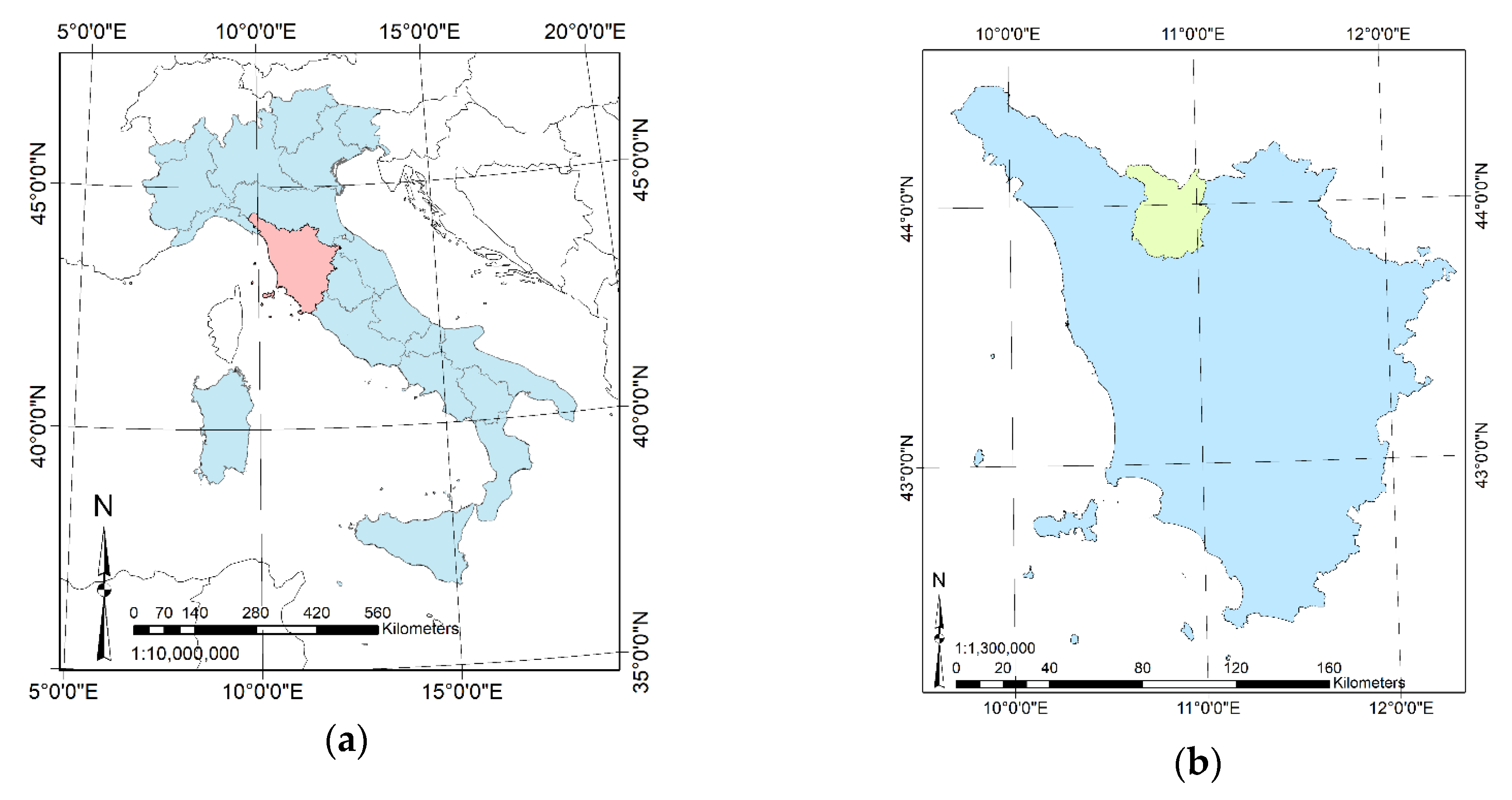
Figure 1. Study area: (a) Italy (light blue) and the Tuscany Region (pink); (b) Tuscany Region (light blue) and the Province of Pistoia (light green); (c) Study area: elevation, river network, and two-lane rural roads crossing the area.
Remotesensing 12 03976 g001aRemotesensing 12 03976 g001b
Figure 2. Land use classification of the city of Pistoia. Most of the nurseries (blue) are located around the city center.
Remotesensing 12 03976 g002aRemotesensing 12 03976 g002b
Figure 3. The workflow of the proposed approach.
Remotesensing 12 03976 g003
Figure 4. Output target: (a) Persistent Scatterer (PS) measurements over the study area (52,257 PSs); (b) PS density.
Remotesensing 12 03976 g004
Figure 5. Surface motion map over the city center of Pistoia.
Remotesensing 12 03976 g005
Figure 6. Tree pruning process.
Remotesensing 12 03976 g006
Figure 7. Scatterplots of the training and testing phases: (a) Regression Tree (RT); (b) SVM; (c) BRT; (d) RF.
Remotesensing 12 03976 g007aRemotesensing 12 03976 g007b
Figure 8. Taylor Diagram of the MLAs (Standard Deviations in black, R2 in blue, RMSE in green, Reference Population in red).
Remotesensing 12 03976 g008
Figure 9. Surface motion mapping over the study area: (a) RT; (b) SVM; (c) BRT; (d) RF.
Remotesensing 12 03976 g009aRemotesensing 12 03976 g009b
Figure 10. Road condition [mm/year]—Case studies: (a) SR435; (b) SR66_Sud; (c) SR66_Nord.
Remotesensing 12 03976 g010
Table 1. Review of papers addressing environmental-related issues by Machine Learning.
Ref.TopicTaskMLAsPerformance MetricsFeature Selection
[57]Landslide SusceptibilityCLR, LMT, SVM, ANNAUROC, KI, Spec., Sens.VIF
[58]Landslide SusceptibilityCWoE, LR, SVMAUROCPCA, Chi-square test
[59]Landslide SusceptibilityCNB, BLR, RFAUROCVIF, Chi-square test, Pearson Correlation
[60]Landslide SusceptibilityCCART, RFAUROC, KI, Spec., Sens., Prec., Acc., RMSE, MAEVIF
[61]Landslide SusceptibilityCSVMAUROCNo
[62]Landslide SusceptibilityCCARTAccuracyNo
[63]Landslide SusceptibilityCCF, IoE, LRAUROCNo
[64]Landslide SusceptibilityCANNAccuracyNo
[65]Landslide SusceptibilityCANNAUROCNo
[66]Landslide SusceptibilityCSVM, LR, ANNAccuracy, Conf. Mat., AUROCNo
[67]Landslide SusceptibilityCSVMAUROC, KINo
[68]Landslide SusceptibilityCCARTAUROCNo
[69]Landslide SusceptibilityCABSGD, SGD, LR, LMT, FT, SVMSens., Spec., Accuracy, Conf. Mat., AUROC, RMSELSSVM
[70]Landslide SusceptibilityCSVMAUROCNo
[71]Landslide SusceptibilityCFR, LRAccuracy, AUROCNo
[72]Landslide SusceptibilityCSVM, CART, NBSens., Spec., Prec., Accuracy, KI, AUROCNo
[73]Landslide SusceptibilityCSVM, CART, ANFISAUROC5 different datasets have been used
[74]Landslide SusceptibilityCFRAccuracyNo
[75]Landslide SusceptibilityCCART, BRT, RF, GLMAUROCVIF, CART, BRT, RF
[76]Landslide SusceptibilityCRF, LR, LMTSens., Spec., Accuracy, AUROC, RMSE, MAE, F&WNo
[77]Landslide SusceptibilityCSVM, BLR, ADTSens., Spec., Accuracy, AUROC, RMSE, F&WORAE
[78]Landslide SusceptibilityCLMT, LR, NBT, ANN, SVMSens., Spec., Accuracy, AUROC, RMSE, MAEORAE
[79]Landslide SusceptibilityReview paper
[80]Mass Movement Susceptibility (debris flow, landslides, rockfalls)CRF, MARS, MDA, BRTAUROCPearson Correlation
[81]Mass Movement Susceptibility (debris flow, landslides)CLRR2, Conf. Mat.No
[82]Mass Movement SusceptibilityCANN, FR, LRAccuracySI, SDC
[83]Gully erosion by stream powerCMARS, FDA, SVM, RFAUROCVIF
[84]Gully erosion by stream powerCWoE, MARS, BRT, RFAUROCVIF
[85]Gully erosion by stream powerCCF, RFAccuracy, Conf. Mat.VIF
[86]Floods susceptibilityCNB, NBTAUROC, KI, Accuracy, RMSE, MAEVIF, IGR
[87]Floods susceptibilityCWoE-SVM (ensemble)AUROCBSA
[88]Floods susceptibilityCSVM, FRAUROC, KINo
[89]Floods susceptibilityCEBF, LR, EBF-LR (ensemble)AUROCVIF
[90]Groundwater Potential MappingCCART, BRT, RF, EBF, GLMAUROCNo
[91]Groundwater Potential MappingCFR, CART, BRT, RFAUROCNo
[92]Groundwater Potential MappingCSVM, MARS, RFAUROC, F1, Fall., Sens., Spec., TSS, AccuracyLASSO
[93]Groundwater Potential MappingCFR, BRT, FR-BRT (ensemble)AUROC, Spec., Sens.No
[94]Avalanches, rockfalls, and floods susceptibilityCSVM, BRT, GAMTSS, Sens., Spec., AUROCNo
[95]Subsidence modelingCCART, RBDT, BRT, RFTSS, Sens., Spec., AUROCNo
[96]Surface settlement prediction by tunnelingRSVM, ANN, GPRR2, RMSE, MAE, RAE, RRSEWrapper Forward and Backward
[97]Slope stability assessmentC/RSVMAccuracy, R2, RMSE, MAENo
[98]Slope stability assessmentRANN, GPR, MLR, SLR, SVMR2, RMSE, MAE, RAE, RRSENo
[99]Consolidation coefficient of soil predictionRRFR2, RMSE, MAE8 different datasets have been used
[100]Temperature predictionRSVM, ANNMSENo
[101]Prediction of nitrate pollution of groundwater RSVM, KNN, RFR2, RMSE, Taylor DiagramNo
Acronyms of MLAs: CART = Classification and Regression Tree, LR = Logistic Regression, LMT = Logistic Model Tree, SVM = Support Vector Machine, ANN = Artificial Neural Network, WoE =Weight of Evidence, BLR = Boosted Logistic Regression, BRT = Boosted Regression Tree, RF = Random Forest, NB = Naïve Bayes Classifier, NBT = Naïve Bayes Tree, GAM = Generalized Additive Model, GPR = Gaussian Process Regression, MLR = Multiple Linear Regression, SLR = Simple Linear Regression, MARS = Multivariate Adaptive Regression Splines, FDA = Flexible Discriminant Analysis, CF = Certainty Factor, IoE = Index of Entropy, SGD = Stochastic Gradient Descend, FT = Functional Tree, ABSGD = AdaBoost-SGD, FR = Frequency Ratio, ANFIS = Adaptive Neuro-Fuzzy Inference System, BLR = Bayesian Logistic Regression, ADT = Alternating Decision Tree, GLM = General Linear Model, EBF = Evidential Belief Function, MDA = Mixture Discriminant Additive, KNN = K-Nearest Neighbor. Acronyms of Performance Metrics: R2 = Correlation Coefficient, RMSE = Root Mean Square Error, MAE = Mean Absolute Error, RAE = Relative Absolute Error, RRSE = Root Relative Squared Error, AUROC = Area Under the Receiver Operating Characteristic, KI = Kappa-Index, F&W = Friedman & Wilcoxon test, TSS = True Skill Score, F1 = F1-Score, Fall. = Fallout, MSE = Mean Square Error. Acronyms of Feature Selection: PCA = Principal Component Analysis, Corr. Mat. = Correlation Matrix, VIF = Variance Inflation Factors, IGR = Information Gain Ratio, LSSVM = Least-Square SVM, BSA = Bivariate Statistical Analysis, ORAE = One–R Attribute Evaluation, SI = Susceptibility Index, SDC = Standard Deviation Criterion, LASSO = Least Absolute Shrinkage and Selection Operator.
Table 2. Descriptive statistics of the numerical input features.
Input FeatureUnitRef.Min.Max.MeanSt. Dev.Skew.Kurt.
Elevation[m][83]12.191792.46130.93219.372.716.99
Aspect[rad][57]0.006.283.011.400.06−0.42
Slope[rad][86]0.001.210.060.102.9012.23
Curvature[rad][86]−1.130.830.000.02−2.27473.25
Convergence Index[-][84]−100.00100.000.9115.750.237.80
Slope-Length[m][83]0.001853.3895.08130.403.1115.55
Topographic Position Index[-][94]−40.3730.330.052.590.0722.01
Vector Ruggedness Measure[-][94]0.000.570.000.0111.38247.11
Terrain Ruggedness Index[-][59]0.0018.720.460.834.8251.54
Average Yearly Rainfall[mm/year][61]957.791781.721092.22125.832.477.36
Topographic Wetness Index[-][83]4.3219.9911.052.140.12−0.18
Stream Power Index[m2/m][61]0.0053,146.60146.48749.5825.931066.99
River Density[river/km2][83]0.003.250.850.430.510.35
Distance from rivers[m][86]0.001951.67401.78315.720.990.52
Earthquake susceptibility[magn.] 1.321.921.600.16−0.40−1.00
Distance from landslides[m] 0.006704.571296.571278.211.110.68
Diffusive Yearly Solar Radiation[kWh/m2][119]0.671.010.990.03−2.819.57
Direct Yearly Solar Radiation[kWh/m2][119]0.105.864.420.28−0.4214.64
Wind Exposition[-][94]0.791.290.950.051.915.98
Content of Sand of the subsoil[%] 6.6067.0037.5312.440.09−0.61
Content of Silt of the subsoil[%] 16.6065.3645.5910.440.100.56
Content of Clay of the subsoil[%] 2.8551.5816.917.031.411.70
Content of Organic of the subsoil[%] 0.658.241.450.723.3419.88
Table 3. Descriptive statistics of the categorical input features.
Input FeatureTypeNumber of Categories
Drainage Capacity of the soilOrd6
Flood susceptibilityOrd4
Erosion susceptibilityOrd7
Landslide susceptibilityOrd5
Land UseCat39
Area TypeBin2
Table 4. Wrapper feature selection process: (1) Forward, (2) Backward, and (3) Bi-directional.
Wrapper Feature Selection Approaches
Wrapper TypeForward Feature SelectionBackward Feature SelectionBi-Directional Feature Selection
Selected AttributesElevationElevationElevation
RainfallRainfallRainfall
Distance from riversDistance from riversDistance from rivers
Distance from landslidesDistance from landslidesDistance from landslides
Earthquake susceptibilityEarthquake susceptibilityEarthquake susceptibility
Type of areaType of areaType of area
River densityRiver densityRiver density
Silt contentSilt contentSilt content
Sand content Clay contentSand content
Org content
Starting setNo attributesAll attributesNo Attributes
Iterations338424464
RMSE0.3930.3900.391
Table 5. Goodness-of-Fit and Predictive Performance of the Machine Learning Algorithms (MLAs).
Single Learners
RTSVM
TrainingTestingTrainingTesting
St. Dev. [mm/year]2.03242.01732.03602.0504
R20.97660.90120.98790.9500
RMSE0.31460.65700.22660.4672
MAE0.16640.34700.09370.2658
Ensemble Learners
BRTRF
TrainingTestingTrainingTesting
St. Dev. [mm/year]2.05342.01451.97771.9555
R20.99980.95570.98280.9466
RMSE0.03020.44010.26940.4829
MAE0.01610.26410.15720.2823
Number of instances in the training set = 36,580 (70%). Number of instances in the test set = 15,677 (30%). St. Dev. of the reference population in the training set = 2.0566 mm/year. St. Dev. of the reference population in the test set = 2.0900 mm/year.
Table 6. Predictor Importance of the MLAs and comparison with wrapper approaches.
Input FeaturesPredictor ImportanceForward WrapperBackward WrapperBi-Directional Wrapper
Organic Content70.23
Clay content43.86
Flood Susceptibility41.4
Silt Content41.29
Distance from Landslides37.32
Earthquake Susceptibility35.12
Drainage Capacity34.34
Landslide Susceptibility27.8
Erosion Susceptibility26.24
Rainfall22.48
Sand Content20.37
Diffusive Solar Radiation19.01
Land Use18.83
River Density12.01
Elevation11.08
Type of Area9.63
Distance from Rivers8.17
WE7.77
TRI4.89
Direct Solar Radiation3.7
Slope3.37
VTR3.31
Aspect2.81
SPI2.27
TWI1.88
TPI1.81
Slope Length1.72
Curvature1.28
CI1.19
Table 7. Performance of MLAs trained with all the input features.
Single Learners
RTSVM
TrainingTestingTrainingTesting
St. Dev. [mm/year]2.03261.97940.62730.61107
R20.91620.83350.28350.2625
RMSE0.59560.84481.75311.7733
MAE0.37470.51650.95320.9652
Ensemble Learners
BRTRF
TrainingTestingTrainingTesting
St. Dev. [mm/year]1.99721.8891.89451.8078
R20.98500.89870.97240.8709
RMSE0.25240.65830.33510.7499
MAE0.18680.39400.19370.4037
Publisher’s Note: MDPI stays neutral with regard to jurisdictional claims in published maps and institutional affiliations.