Abstract
Abundant data sets produced from long-term series of high-resolution remote sensing data have made it possible to explore urban issues across different spatiotemporal scales. Based on a 40-year impervious area data set released by Tsinghua University, a method was developed to map the speed and acceleration of urban built-up areas. With the mapping results of the two indices, we characterised the spatiotemporal dynamics of built-up area expansion and captured different types of expansion. Combined with socioeconomic data, we examined the temporal changes and spatial heterogeneity of driving forces with an ordinary least square (OLS) model and a panel data model, as well as exploring the environmental effects of the expansion. Our results reveal that China has experienced drastic urban expansion over the last four decades. Among all cities, megacities and large cities in eastern China, as well as megacities in central and northeast China have experienced the most dramatic urban expansion. A growing number of cities are categorised as thriving, which means that they have both high expansion speed and acceleration. The overall driving force of urban expansion has significantly increased. More specifically, it was associated with population increase in the early stages; however, since 2000, it has been substantially associated with increases in GDP and fixed asset investments. The major driving factors also differ between regions and urban sizes. Urban expansion is identified as being closely associated with environmental deterioration; thus, speed and acceleration should be included as key indicators in exploring the environmental effects of urban expansion. In summary, the results of the presented case study, based on a data set of China, indicate that speed and acceleration are useful in analysing the driving forces of urban expansion and its environmental effects, and may generate more interest in related research.
1. Introduction
As a consequence of the processes of urbanisation and socioeconomic development, urban area has expanded significantly worldwide. In the last few decades, dramatic increases in built-up areas have been experienced globally [1,2], with a total built-up area of 797,076 km2 in 2018, 1.5 times that in 1990 [3]. As urbanisation continues, the demand for land is expected to increase [4]. It is forecasted that urban land cover will increase by 1.2 million km2 by 2030, nearly tripling the global urban land area circa 2000 [5]. Such expansion is becoming increasingly unsustainable, with urban areas expanding much faster than the population [6], especially in India, China, North America, and Europe [7]. Analyses have suggested that, due to the decrease in urban population densities, an estimated 125,000 km2 of land was converted to urban land-uses that could have otherwise remained in cultivation or as natural vegetation [7]. Though occupying only a small proportion of the global land cover, the expansion of built-up area significantly affects Earth system processes and, thus, has tremendous ecological and environmental consequences, such as arable land loss [7,8,9], biodiversity loss [10,11], local and regional climate change [12,13,14], and higher air pollution concentrations [15,16]. The scarcity of land makes better governing a necessity, promoting sustainable planning [17]; for which, studies focusing on understanding the spatiotemporal characteristics of built-up area expansion at different levels is essential.
In China, the expansion of built-up areas has its own characteristics, due to the joint effects of the government and the market. Since the reform and opening up in 1978, the pace of urbanisation in China has increased significantly. In 2015, China became the country with the most built-up area in the world [3]. Due to differences in market attractiveness and policy emphasis, there has been a significant heterogeneity in the expansion of built-up areas over time and across regions. Temporally, the expansion speed increased in the 2000s [18,19,20], while the change in the 2010s remains controversial, owing to the study areas and data sources [21,22]. Spatially, expansion has mainly been observed in coastal China, with Beijing–Tianjin–Hebei (BTH), the Yangtze River Delta (YRD), and the Pearl River Delta (PRD) experiencing the largest expansion agglomeration [19,23,24]. Cities with larger size tend to expand at higher speed [25]. However, owing to the difficulty in obtaining urban expansion information over multiple years on a large spatial scale, studies with a national coverage and a long time period—in particular, covering the whole time span since China’s marketisation—is rare.
Statistic data and remote sensing data are the main data sources in studies of built-up area expansion, while the latter has fine spatial information and can help analysing the change in urban built-up areas objectively from multitemporal images. Landsat data is widely used, with impervious area identified based on surface reflectance. However, with a 30 m spatial resolution, it has difficulty in covering a large spatial scale. While night-time light (NTL) data is mainly at medium-low resolution and frequently used in analysing urban expansion at large scales. Of which, Defense Meteorological Satellite Program and Operational Linescan System (DMSP-OLS) covers the longest time span (from 1992 to the present), is of interest by researchers. With DMSP-OLS data, the built-up area expansion based on night light intensity can be summarised. The national rapid growth and great disparities among regions are consistent with studies using Landsat data and statistic data [26,27,28,29,30]. Hot points are also prone to concentrate around BTH, YRD, PRD, and provincial capitals, which are the highpoints of urban growth as well [28]. DMSP-OLS data can also help identify the general formation of the strategic urban pattern characterised by two horizontal axes and three vertical lines [29]. Generally, night-time light data directly reflects socioeconomic development and human activities and can help in identifying the expansion dynamics at the national scale.
To characterise the pattern of built-up area, numerous landscape indices have been developed, such as landscape shape index (LSI) [2], largest patch index [25], and fractal dimension index [24]. Researchers have used these indices to quantify the geometric and spatial properties of categorical map patterns but have seldom used them to obtain information about the dynamic change processes of landscape patterns. Indices for quantifying urban dynamics at two or more time points are essential. Researchers have used indices to capture information on temporal changes of built-up areas, including dynamic degree [19], (annual) expansion areas [20,25,31], and (annual) expansion rates [20,25,32], which have most frequently been used to observe temporal changes in built-up areas, thus representing the speed of expansion. However, the spatiotemporal pattern of changes in speed has never been mapped, which can be interpreted as the change in driving forces of built-up area expansion [20]. This paper develops a new index, acceleration, to measure the change in expansion speed, to represent the change in driving forces. Speed and acceleration, together, can give us insight to better understand spatiotemporal land-use dynamics in fast-growing regions. It is expected that speed and acceleration can be used to identify the characteristics of temporal changes of a certain landscape (in this study, we selected built-up area) using multitemporal remote sensing data.
In this paper, using the multitemporal built-up area data with Landsat imagery and night-time light (NTL) data as data sources, we mapped and quantified the dynamics of built-up area expansion in China over the past four decades using expansion speed and acceleration as indicators, as well as investigating the driving forces and environmental effects of built-up area expansion, based on the mapping results. We have four objectives: (1) to develop a data set of expansion speed and acceleration at fine resolution over 40 years; (2) to find new information from the mapping of the two indicators, including the spatiotemporal characteristics of built-up area expansion and its differences between regions and urban sizes, and expansion types from the perspective of temporal changing dynamic; (3) to examine the driving factors and their spatiotemporal changes; (4) to explore the relationships between different expansion indicators and environmental changes.
2. Materials and Methods
2.1. Data Sources
Built-up area data from 1978 to 2017 were obtained from the data set produced by Gong et al. at Tsinghua University [33]. These data provide timely, accurate, and frequent information, including the first annual human settlement map from 1985 to 2017 with a circa 1978 map produced at the beginning of the economic reform in China. Landsat imagery is the main source in this project, with an ancillary data set of night-time light (NTL) data. The spatial resolution in 1978 was 60 m, while the spatial resolution during 1985–2017 was 30 m. The overall accuracies of this data have reached more than 90% [33]. With this data set, we can observe spatiotemporal changes over the 40 years. In addition, the long timespan of this data set makes it possible to calculate the expansion speed and acceleration in different periods during its long timespan. In the meantime, the global artificial impervious area (GAIA) project (to which it belongs) has also produced a global data set of built-up areas between 1985 and 2018 [34], such that the method developed in this paper is also suitable to further explore worldwide expansion dynamics and generate more results across different spatial scales. The data were downloaded from http://data.ess.tsinghua.edu.cn.
Socioeconomic statistical data were used to analyse the social and economic drivers of urban expansion, which were collected from provincial and prefectural statistical yearbooks (1978–2017). Environmental data from the China Environmental Statistical Yearbook (1998–2017) were used to examine the relationship between built-up area expansion and environmental changes. The data are described in Table 1.

Table 1.
Data in this study.
2.2. Methods
The workflow (Figure 1) involves four parts (or steps). The first step is computing and mapping the speed and acceleration of built-up area expansion. The second step incorporates some new perspectives, in order to characterise built-up area expansion based on the mapping results, including analysis of the spatial correlation of expansion and its spatiotemporal differences by region and urban size, as well as identifying the expansion type based on the speed and acceleration. The third step includes estimation of the impacts of core socioeconomic drivers and their spatial and temporal heterogeneity. The fourth step involves exploring the relationship between environmental factors and built-up area expansion indicators.
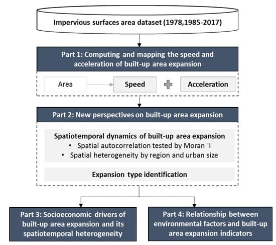
Figure 1.
The workflow of the mapping and analysis process.
2.2.1. Mapping Built-Up Area Expansion
The mapping is integrated using 5 × 5 km grids and involves five steps (Figure 2): (1) creating a fishnet and segmenting the image with grids; (2) within each grid, converting the raster to points, where each point represents a piece of land built in a specific year; (3) counting the number of built-up points in 1978, 1990, 2000, 2010, and 2017, and calculating the relevant area; (4) computing the speed and acceleration in different periods; (5) integrating the calculation results of individual grids to obtain the overall mapping results of the speed and acceleration. Spatially, the results contain the expansion characteristics at a 5 km resolution; temporally, the changes in different periods can also be detected.
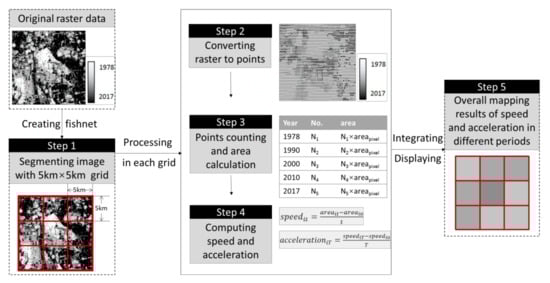
Figure 2.
Mapping of speed and acceleration based on data processing.
The formulae for speed and acceleration in step 4 are as follows:
where areait and areai0 are the built-up areas of grid i in the final and initial year of period t, respectively; SpeediT and Speedi0 are expansion speeds of grid i in the final and initial year of period T, respectively.
When counting on a city-by-city basis, we averaged each of these indicators and counted the built-up area expansion per square kilometre of land; thus, the modified indices can be used to compare expansion amongst different regions and urban sizes.
2.2.2. Analysis of the Spatial Autocorrelation and Strata of Built-Up Area
We utilised a global Moran’s I test to measure spatial autocorrelation of expansion speed and acceleration. Positive and significant values of the global Moran’s I indicate the presence of positive spatial autocorrelation of built-up area expansion, where high values and low values of expansion are spatially clustered. In contrast, negative and significant values of the global Moran’s I suggest the spatial distribution of high values and low values of expansion speed and acceleration are more spatially dispersed. If the global Moran’s I is not statistically significant, the spatial distribution is considered random. The formula for Moran’s I is as follows:
where n is the number of spatial units indexed by i and j, and wij is a matrix of spatial weights with zeros on the diagonal.
In terms of heterogeneity, we analysed the urban expansion characteristics in different regions and for different urban sizes. According to the differences in socioeconomic development, the mainland of China was zoned into four economic zones: eastern, central, western, and northeast regions. We also considered the differences in urban expansion between cities with various urban sizes. According to a document recently released by China’s State Council (2014), cities can be classified into five categories and seven levels, based on the resident population scale in urban areas, which are small cities A, small cities B, medium cities, large cities A, large cities B, super cities, and megacities [35]. To simplify the city classification, we classified small cities A and small cities B as small cities; large cities A and large cities B as large cities; super cities and megacities as megacities. This classification was based on the urban population data in 2017 (Table 2). The administrative levels of cites in our study were prefecture-level or above, including direct-controlled municipalities, subprovincial cities, and prefecture-level cities. Based on the above classifications, differences in built-up area expansion between different regions and urban sizes were calculated and compared.
Table 2.
Description of populations in different cities.
2.2.3. Characterising Expansion Types Based on Speed and Acceleration
We proposed a new way to categorise cities, in order to highlight a subset of cities from the perspective of land expansion. Categorising cities by their expansion speed and acceleration helps to identify both the cities that are expected to continually expand at a high growth speed and cities lacking sustained driving forces. The use of these two indicators allowed us to assign cities into four categories: thriving, stabilising, emerging, and struggling (Figure 3). We defined the four categories of cities as follows:
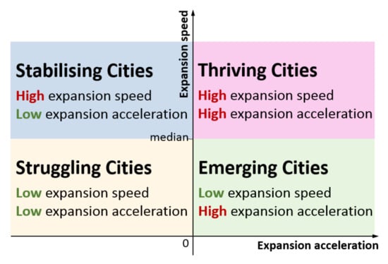
Figure 3.
Categorisation of cities by built-up area expansion speed and acceleration.
Thriving cities have high expansion speed and high acceleration. They are likely to experience sustained built-up area expansion with increased infusion of development resources, such as capital and policy. Stabilising cities have high expansion speed and low acceleration. These cities have entered a post-rapid expansion period, in which their driving forces tend to decrease. Emerging cities have low expansion speed and high acceleration. They are expected to face an increase thereafter. Struggling cities have low speed and low acceleration. They are usually under-developed cities, without any favour of policy or capital.
2.2.4. Estimation of the Driving Factors
To estimate the impact of selected socioeconomic factors in different periods and spatial strata, a linear OLS model and a panel data model were used. Economic development, population growth, and fixed asset investment were considered to have effects on built-up area expansion, with industrial structure as a mediator of the effect of economic development on built-up area expansion (Figure 4). Fixed asset investment in real estate, infrastructure, and manufacturing buildings can directly result in built-up area expansion and indirectly in the facilitation of economic development. Economic development can boost demand, thus expanding the scale of production and attracting more projects, leading to built-up area expansion. It also provides more employment, thus increasing the total population and having a long-term influence on built-up area expansion [36]. The industrial structure is assumed to influence the effect of economic development on built-up area expansion, owing to the different land demand of secondary and tertiary industry development [36]. To test the relationships, four indicators—namely, change in GDP, change in population, total amount of fixed asset investment (using average fixed asset investment at the start and end of the year as an indicator), and proportion of secondary industry production in GDP change—were employed.
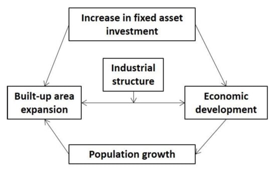
Figure 4.
The conceptual framework of built-up area expansion in China.
Linear OLS regression was used to estimate the different effects of socioeconomic factors in different periods, formulated as follows:
where BUCi is the dependent variable, the annual change in built-up area for each city; GDPi, POPi, FAIi, and GDP2i are the changes in GDP and population, averaged fixed asset investment, and proportion of secondary industry production in GDP change for each city, respectively; is the error term.
The ordinary least squares method was used to determine the line of best fit for a set of data, with general form:
To investigate the spatial heterogeneity of the mechanisms, in terms of regional distribution and urban size, we set eight subgroups (in terms of region and urban size). As the data were multidimensional data of an observation measured repeatedly over time (i.e., with variation along city and time dimensions), the panel data model was used. The basic form of the panel data model is:
where BUCit is the dependent variable, the annual change in built-up area in each period for each city; GDPit, POPit, FAIit, and GDP2it are the changes in GDP and population, averaged fixed asset investment, and proportion of secondary industry production in GDP change in each period for each city, respectively; μi and εit are error terms. εit represents the unobservable factors that vary with the cross-section and time, while μi represents the unit-specific error term. This term differs between units but, for any particular unit, its value is constant. A least squares dummy variable (LSDV) model was used to estimate the parameters. In a fixed effect model, the heterogeneity across cities is captured in the constant term while, in the random effect model, heterogeneity also appears across years.
We used an F test to test the differences across cities, with the hypothesis that the constant terms were all equal. The F ratio used for this test was
where LSDV indicates the dummy variable model and the subscript Pooled indicates the pooled or restricted model with only a single overall constant term. The significance of the F test implies that differences exist among cities; therefore, the pooled model was rejected.
The modified Hausman test was employed to differentiate between the fixed effects model and random effects model in the panel data, with formula as follows:
where and are the root mean square errors in the fixed effect model and random effect model, respectively. If the null hypothesis is rejected, the fixed effects model is appropriate. Fixed effects models take into account the differences between cities, while a random effects model takes into consideration these individual variations, as well as time-dependent variations. The model eliminates biases from variables that are unobserved and change over time.
To validate the regression model, we trained the panel data model to test its stability. As our panel dataset has four periods, in the case of total samples, we created our training model by leaving four out each time (when balanced), which is the same city in different periods. Additionally, because what we are interested in is whether a model can fit for all cities rather than its prediction ability in time series, we used a leave-one-out cross-validation (LOOCV) in each period. In LOOCV, each learning set was created by taking all samples except one, the test set being the sample left out. Thus, for n samples, we obtained n different training sets and n different test sets. The resulting output listed the RMSE and MAE, along with a pseudo R-squared type measure. The results imply the accuracy and performance of the regression result in a new data set.
2.2.5. Relationship between Environmental Factors and Built-Up Area Expansion Indicators
A Spearman’s correlation test was used to determine the relationship between built-up area expansion and environmental change, which is a nonparametric measure of rank correlation that assesses how well the relationship between built-up area and values of environmental factors in each year can be described using a monotonic function. The formula is as follows:
where di is the difference in the ordering of the two variables and n is the number of observations.
3. Results
3.1. Mapping Results of the Speed and Acceleration of Built-Up Area Expansion
The mapping results show that the areas of high expansion speed and acceleration have enlarged dramatically (Figure 5). The coastal region and some large cities in central China are areas with rapid expansion speed. Large urban agglomerations, such as Beijing–Tianjin–Hebei (BTH) and the Yangtze River Delta (YRD), have experienced accelerating expansion in the last 40 years. Acceleration in the North China Plain and northeast region increased significantly between periods 3 and 4. Detailed information at the city level can also be provided in the mapping results. Taking Shanghai as an example, the rapidly expanding area has changed from the central region in the 1990s to the outlying new towns in the 2010s, with its acceleration having a toroidal structure.
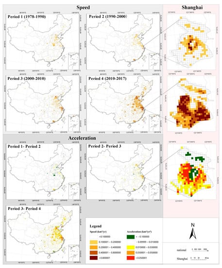
Figure 5.
Mapping results of expansion speed and acceleration at the national and city level.
3.2. Temporal Variation of Built-Up Area Expansion at the National Scale
According to the calculation based on the mapping results, the built-up area expanded significantly, from 19,434 km2 in 1978 to 245,362 km2 in 2017 (Figure 6). The 40 years were divided into four periods, based on which the speed and acceleration of expansion were observed. The results show that the highest annual growth occurred between 2010 and 2017, with an expansion speed of 13,808 km2/yr—3.38 times more than in the previous time period—followed by 2000–2010 (5391 km2/yr), 1990–2000 (3495 km2/yr), and 1978–1990 (3384 km2/yr). The accelerations were 10.1, 187.6, and 937.4 km2/yr2, respectively, indicating a considerable increase in overall driving forces, especially after 2010.
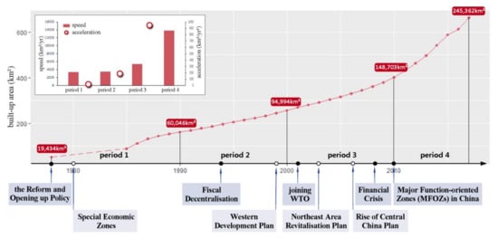
Figure 6.
Built-up area expansion in China between 1978 and 2017.
In terms of spatial distribution, the values of Moran’s I were positive, and the spatial dependence was highly significant over the four decades, indicating the spatial clustering of expansion speed and acceleration (Table 3). The Moran’s I values for expansion speed were 0.566, 0.667, 0.603, and 0.617 in the four respective periods, with the highest spatial dependence in the 1990s. There was a gradual increase in spatial clustering for expansion acceleration, with Moran’s I values of 0.293, 0.454, and 0.543, respectively, indicating an increase in spatial clustering of socioeconomic resources driving built-up area expansion.
Table 3.
Moran’s I index of expansion speed and acceleration in different periods.
3.3. Comparison among Regions and Urban Sizes
Comparison of urban expansion amongst various regions and urban sizes enables more insights into urban expansion (Figure 7a, Table 4). Between 1978 and 2017, built-up areas in all regions increased (Figure 7b). The eastern region exhibited the highest proportion of built-up area, followed by the central region, the northeast region, and the western region, respectively. The average expansion speeds were 3098, 1375, 89, 786 m2/yr per square kilometre of land in the eastern, central, western, and northeast regions, respectively. The expansion speed in the eastern region increased continually for 40 years, while the speed in central and northeast regions remained almost unchanged until 2010. In terms of acceleration, the eastern region had the highest acceleration in all periods. During the first two periods, only the eastern region had a positive acceleration, reflecting the development priority under limited resources. The acceleration of the eastern region from the 1990s to the 2000s was still much higher than the other regions (118 m2/yr2 vs. 33.1, 4.3, and 17.5 m2/yr2 per square kilometre of land). The last two periods saw significant increases in acceleration in all regions.
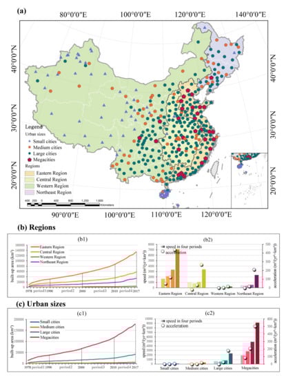
Figure 7.
Sample city identification and built-up area expansion: (a) sample city identification of different regions and urban sizes; (b) differences in built-up area expansion by region, based on comparison of built-up area, speed, and acceleration; (c) differences in built-up area expansion according to urban size, based on comparison of built-up area, speed, and acceleration.
Table 4.
Comparisons of the area, speed, and acceleration by regions and urban sizes.
Figure 7c displays the characteristics of urban expansion for differently sized urban cities. The variation is quite large in all three indicators, with megacities ranking first, followed by large cities, medium cities, and small cities. The average expansion speeds were 4126, 953, 134, and 25 m2/yr per square kilometre of land for mega, large, medium, and small cities, respectively. Acceleration prior to 2010 was mainly observed in megacities, indicating the concentration of development resources in major growth poles.
To further analyse the differences in urban expansion based on urban size within different regions, we summarise the regional and urban size differences in Appendix A. The results show that different-sized cities in the eastern region have experienced sustained urban expansion after the reform and opening up, while expansion in other regions was mainly concentrated in megacities, with megacities and large cities accelerating after 2000.
3.4. Type of Built-Up Area Expansion
The number of thriving cities increased by approximately 50% since 2000 (Figure 8). As a result of rational investment, the changes in speed and acceleration were consistent, with no emerging city being identified as particularly noteworthy. The spatial and temporal pattern changed over the 40 years. The thriving cities between 1978 and 1990 were mainly concentrated in coastal China and the North China Plain, with the highest speed and acceleration observed in the Pearl River Delta (PRD; see Figure 9). In the 1990s, the number of thriving cities in these regions increased; the highest expansion speed occurring in the PRD, and the fastest acceleration occurring in the Yangtze River Delta (YRD) and Beijing–Tianjin–Hebei (BTH). In the 2000s, many cities in the central and northeast regions, and some of the major cities in the western regions, were also categorised as thriving. After 2010, acceleration failed to continue in some megacities in the PRD; thus, these cities became stable following 20 years of thriving development.
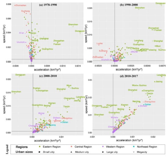
Figure 8.
Categorisation results of expansion type in different periods based on speed and acceleration: (a) expansion type categorisation in 1978–1990; (b) expansion type categorisation in 1990–2000; (c) expansion type categorisation in 2000–2010; (d) expansion type categorisation in 2010–2017.
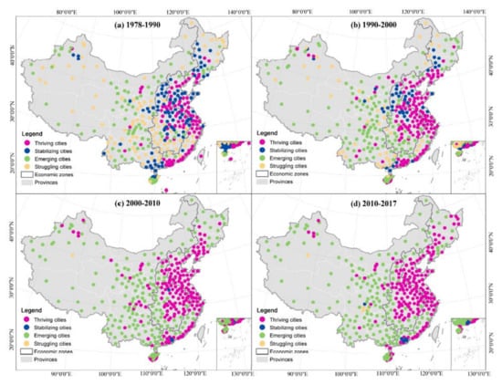
Figure 9.
Distribution of thriving, stabilising, emerging, and struggling cities in different periods: (a) distribution of different types of cities in 1978–1990; (b) distribution of different types of cities in 1990–2000; (c) distribution of different types of cities in 2000–2010; (d) distribution of different types of cities in 2010–2017.
In addition, in mature urban agglomerations, the neighbouring cities, such as Zhongshan, Foshan, Wuxi, and Suzhou expanded concurrently. Cities in other agglomerations were distributed independently in the axes, indicating the stage of development in the growth pole.
3.5. Socioeconomic Drivers behind Built-Up Expansion
After mapping and comparing the spatiotemporal changes in driving forces indicated by acceleration, we further explored the specific drivers, in terms of the period (Models 1–4), region (Models 5–8), and urban size (Models 9–12). The results of F test are significant all the time, indicating the difference among cities, so that pooled model is rejected. The modified Hausman test indicated that the fixed effects model performed better, with the exception of Models 5 and 12. Thus, Models 6–11 were based on the fixed effects model, while Models 5 and 12 were based on the random effect model.
The results of the total samples with a panel data model showed that changes in fixed asset investment were positively correlated with built-up area expansion (Model 0 in Table 5). However, the effects of different factors vary in different periods (Model 1–4 in Table 6). In the early period of the reform and opening up, built-up area expansion was mainly related to population growth. In the 2000s, the increase in GDP and fixed asset investment were significantly related to built-up area expansion, where the proportion of secondary industry production strengthened the effect of GDP. After 2010, fixed asset investment had a significantly positive effect, while the proportion of secondary industry production diminished the effect of GDP.
Table 5.
Results of panel data models.
Table 6.
Results of linear OLS models.
The drivers varied, in terms of region and urban size. In the eastern region, population growth, fixed asset investment, and secondary industry production were positively related to built-up area expansion. The central region had a significant relationship with fixed asset investment. In the western region, GDP and fixed asset investment were significantly related to built-up area expansion, where the negative effect of GDP was mitigated with higher secondary industry production. In the northeast region, fixed asset investment was positively related, and the secondary industry production played a negative role in mediating the effect of GDP.
Cities of different sizes experienced different expansion paths. In small cities, population played a negative role. In medium cities, fixed asset investment was a positive driver. In megacities and large cities, GDP and fixed asset investment were positively related to built-up area expansion; whereas, in large cities, the proportion of secondary industry production diminished the effect of GDP.
The validation result indicates that the modelling is relatively stable with the panel data at national scale, with outliers in certain cities (Figure 10). Despite the relatively small adjusted R-square, we can say that the model is reliable and applicable. The RMSE, MAE, and pseudo R-squared in each period are listed in Table 7. They can serve as a comparison for future research.
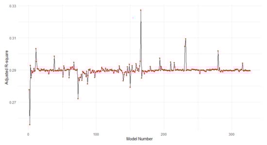
Figure 10.
Adjusted R-square in different training datasets.
Table 7.
Results of cross-validation.
3.6. The Environmental Effects of Built-Up Area Expansion
The built-up area continued to rise between 1990 and 2017. At the same time, wastewater discharge increased from 3.54 billion tons in 1990 to 7.35 billion tons in 2015, with an average annual increase of 3.0%. The average area of natural reserves showed a decreasing trend, especially after 2001, from 8.37 to 5.35 km2 in 2017, with an average annual decrease of 2.8%. Industrial waste gas emissions revealed a rising trend, with the greatest increase occurring between 2000 and 2010.
The change in wastewater discharge, industrial waste gas emissions, and average area of natural reserves was consistent with that of built-up area expansion (Figure 11a). The Spearman’s correlation coefficient passed the significance test and the coefficients between built-up areas and industrial waste gas emission, wastewater discharge, and average area of natural reserves were 0.997, 0.997, and −0.989, respectively. In terms of speed, the growth speed of environmental factors was lower than that of built-up area after 2010 (Figure 11b), showing an opposite acceleration direction. Taking industrial waste gas emissions as an example, different characteristics were shown in three periods. In the 1990s, its growth trend was similar to that of built-up areas. In the 2000s, there was a significant increase in its growth rate, becoming much higher than that of built-up areas, mainly due to industry-driven expansion [20]. Along with the industrial structural transformation and the introduction of clean production policies, its growth rate slowed after 2011.
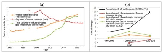
Figure 11.
Relationship between built-up area expansion and environmental factors: (a) dynamics of built-up area expansion and environmental factors; (b) comparison between speed of built-up area expansion and environmental factors.
4. Discussion
4.1. Mapping Results of the Speed and Acceleration of Built-Up Area Expansion
With the multitemporal impervious area data set from Gong et al. [33], the spatiotemporal dynamics of built-up areas were assessed at a 5 × 5 km resolution. It provides us with the expansion of built-up area at 34 time points (1978, 1985–2017). Thus, it is possible to detect the temporal change thoroughly. Corresponding with this characteristic of the data source, we chose speed and acceleration as indices to detect the spatiotemporal change in built-up area. We produced a new data set, mapping the expansion speed and acceleration over the four decades with fine spatial resolution. It can indicate the temporal changes since marketisation in China and the spatial pattern of built-up areas in different periods. Using the acceleration indicator, the spatiotemporal dynamics of driving forces were discerned. The driving forces of built-up area expansion were found to be highly concentrated in the main agglomerations in coastal China. More and more cities have been expanding with increasing force over the last 40 years, as related to the abundant development resources and policies targeting balanced development.
Detailed information at the city scale can also be recognised in the mapping results. This provides information on the change in urban structure, system, and expansion direction, by displaying areas with intensified speed and acceleration. Using the data set we have produced, further research on different spatial scales can be carried out.
4.2. New Perspectives from the Mapping Results
4.2.1. Built-Up Area Expansion Dynamics on the National Scale and in Subgroups
The temporal change of speed and acceleration results showed that the driving forces of built-up area expansion grew dramatically, especially in the early part of the 21st century, which was affected by economic development and national policies. The socioeconomic development in the 20th century in China was not sufficiently abundant to promote the rapid expansion of built-up areas. Due to the deepening of marketisation and globalisation since China’s entrance to the WTO, China has seen a marked increase in the acceleration of its expansion, especially in the eastern region [20,23]. The significant increase in acceleration from 2005 to 2014 is mainly related to the large-scale construction activities in response to the economic downturn, as well as more industrial land being released to attract projects [37]. Beyond a spatial carrier of human activity, the expansion in the 2010s acted more like a tool to facilitate economic growth [38].
From the regional perspective, prior to 2000, positive acceleration was only observed in the eastern region. In this period, the open cities were mainly distributed along the coastline, attracting development resources. Around 2000, regional development policies, including Western Development (1999), Rise of Central China (2006), and Northeast Area Revitalisation (2003), had an impact on expansion acceleration. Thus, the built-up area expansion shifted from single-region clustering to synergistic development at a national scale, with the fastest expansion still in occurring the eastern region, while great expansion also appeared in the central and northeast regions.
In terms of urban size, we found that the speed and acceleration of built-up area expansion were positively related to urban size. This result is in agreement with previous studies that found urban size to positively relate to land urbanisation speed [25,39,40]. We further found that larger cities were more likely to attract more development resources and to have greater driving forces for built-up area expansion, reflecting the siphon effect [41].
4.2.2. Relationship between Speed and Acceleration
The linear relationship between speed and acceleration has gradually strengthened over the past decades. The Pearson correlation coefficient reached 0.877 in the 2010s. This indicates the clustering of built-up areas and its driving forces (i.e., development resources). The higher the expansion speed, the faster the resources are gathered. Further investigation revealed that the two indicators were not always in a linear relationship but, rather, in an inverted U-shape relationship (Figure 12). Cities with higher initial driving forces are more likely to attract resources in the next phase, until reaching a certain threshold, beyond which the increase in management, transportation, and environmental costs will be huge [36]. Our statistics show that this peak appears when the annual growth area is about 1% of the total land.
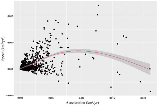
Figure 12.
Relationship between speed and acceleration.
4.3. Temporal Change in Driving Factors and Its Spatial Heterogeneity
The OLS results suggest that the main driver changed from population to economic development and fixed asset investment. In the early stages of the market economy, population growth served as the main driver; that is, built-up area was the spatial carrier for human living, while its effect on population growth within built-up area expansion did not persist all the time [42]. In the 2000s, the economy experienced rapid development after China joined the WTO. The built-up area involved in this process was one of the main factors of production. Investment is a key driver of economic growth, especially after the financial crises in the 2000s and in the 2010s, when exports could not support economic growth. Investment in real estate and infrastructure were encouraged to boost economic growth, thus facilitating the expansion of built-up areas. The industrial structure played different roles in the first two decades of the 21st century. In the 2000s, growth in secondary industries drove built-up area expansion while, in the 2010s, with the transformation of industrial structure, industrial land development slowed down in relatively developed regions [43,44,45], such that cities with a higher proportion of secondary industries had lower expansion speed.
The drivers varied with regions and urban sizes. Fixed asset investment was significantly related to built-up area expansion in all regions, suggesting the important role of investment. Surprisingly, GDP growth was negatively related to built-up area expansion in the western region, suggesting a different development path. The Western Development Program relies primarily on ‘primitive’ economic sectors [46], thus relying less on built-up area expansion. In the Northeast region, with industrial decline, the central cities have mainly focused on developing tertiary industries, while regions with a higher rate of change in secondary industries have experienced a lower rate of expansion.
In terms of urban size, investment did not play a role in the built-up area expansion in small cities, where little fiscal expenditure can be used to construct infrastructure and the market environment does not appeal to companies. The relationship between change in GDP and built-up area expansion is significant in the cases of large cities and megacities while, in smaller cities, too much intervention from the government drives the expansion of built-up areas, leading to a sprawling pattern departing from market rules [47]. This also accounts for the negative effect of population growth in small cities.
The drivers in different regions and urban sizes may also change across periods [48]. Huang et al. found that the driving factor of built-up area expansion in western China has shifted from economic growth in 2000 to industrial structure in 2015 [49]. Chen et al. found that the driving forces in northeast China also varied between 1990 and 2015 [50]. The variation of driving forces in different areas deserve further exploration.
4.4. Application of Built-Up Area Expansion Indicators to Environment Change
Our results show that built-up area expansion is consistent with environmental change, which has been proven by many researchers, suggesting that built-up area expansion has an effect on loss of biodiversity [5,51], inferior air quality [52,53], local and regional climate change [54,55], hydrological cycle alteration [56], and soil quality deterioration [57].
Apart from the general negative relationship, we also found that the growth speed of environmental factors was not always consistent with that of the built-up area. The environmental change slowed down in the 2010s, while the built-up area expansion accelerated. We can interpret, from this enlarging gap, that the relative importance of built-up area expansion for environmental change has decreased. Moreover, the difference in acceleration reflects the effects of other drivers. Here, these mainly comprise the effects of enhanced environmental protection policies. Industrial structure transformation may also play a role. We can preliminarily summarise that the comparison of speed between environmental change and built-up area expansion can provide more information on the extent to which environmental change is influenced by built-up area expansion, while the comparison of acceleration reflects the different changing patterns of driving forces (which come mainly from the government).
In this paper, we did not further investigate the spatial heterogeneity. Existing studies have noted that the relationship between built-up area expansion and environmental outcomes varies with different urban sizes [53], as well as different regions [58]. Therefore, the environmental effects of built-up area expansion speed and acceleration with respect to different spatial strata need to be further explored.
Apart from environmental effects and their related health impacts, further application of these indicators can be explored in future studies, including the dynamic alignment of built-up area with economic development and population growth, in order to test the efficiency and sustainability of built-up area expansion from a longitudinal perspective. Cities in different expansion categories may have different performance in the relationship. The exploration of dynamically changing relationships may be helpful in revealing mechanisms, for which more empirical research is needed.
5. Conclusions
Remote sensing data with long-term series and large geographic coverage make it possible to observe urban expansion from a spatial and temporal perspective. In this study, we used the concept of acceleration to represent the change in driving forces and developed a new data set providing the speed and acceleration of expansion between 1978 and 2017 in China. Based on the mapping results, we investigated the dynamics, driving forces, and environmental effects of built-up area expansion.
We found that (1) there has been considerable growth in the built-up area in China over 40 years, with the eastern region and the megacities experiencing the highest growth speed. Thriving cities, with high expansion speed and acceleration, and which are mainly in the eastern region, were observed. (2) Driving forces tend to increase in rapidly expanding cities and, in analysing the relationship between expansion speed and acceleration, an inverted U-shape relationship was uncovered. (3) The overall driving forces increased dramatically over the four analysed decades. The main drivers changed from population to economic development and fixed asset investment. The driving forces and drivers varied amongst regional distribution and urban size. (4) The environmental factors changed consistently within built-up areas. The difference in speed reflects changes in driving effect, while the difference in acceleration reflects the roles of other drivers.
In this study, we developed a method for mapping the speed and acceleration of urban built-up areas. The combination of these two indicators was shown to be useful for identifying expansion dynamics and changes in driving forces, with potential for further application in the study of environmental effects. They are suitable for longitudinal data and we hope that they will be used to generate more interest in related subjects or on different scales.
Author Contributions
Conceptualisation, X.L.; methodology, Y.J. and X.L.; software, Y.J.; validation, X.L.; formal analysis, Y.J.; investigation, Y.J.; resources, P.G.; data curation, Y.J.; writing—original draft preparation, Y.J.; writing—review and editing, Y.J., X.L., and L.W.; visualisation, Y.J.; supervision, L.W.; project administration, L.W.; funding acquisition, L.W. and X.L. All authors have read and agreed to the published version of the manuscript.
Funding
This research was funded by National Natural Science Foundation of China, grant numbers 41671444, 41871359, and 52078349.
Acknowledgments
We thank Gong Peng’s team at Tsinghua University for data support.
Conflicts of Interest
The authors declare no conflict of interest.
Appendix A

Figure A1.
Differences in urban expansion by urban size within different regions.
Figure A1.
Differences in urban expansion by urban size within different regions.

References
- Seto, K.C.; Fragkias, M.; Güneralp, B.; Reilly, M.K. A Meta-Analysis of Global Urban Land Expansion. PLoS ONE 2011, 6, 23777. [Google Scholar] [CrossRef] [PubMed]
- Zhang, Q.; Seto, K.C. Mapping urbanization dynamics at regional and global scales using multi-temporal DMSP/OLS nighttime light data. Remote Sens. Environ. 2011, 115, 2320–2329. [Google Scholar] [CrossRef]
- Gong, P.; Li, X.; Wang, J.; Bai, Y.; Chen, B.; Hu, T.; Liu, X.; Xu, B.; Yang, J.; Zhang, W.; et al. Annual maps of global artificial impervious area (GAIA) between 1985 and 2018. Remote Sens. Environ. 2020, 236, 111510. [Google Scholar] [CrossRef]
- European Environment Agency. Urban Sprawl in Europe: The Ignored Challenge; European Environment Agency, European Commission, Eds.; European Environment Agency: Copenhagen, Denmark, 2006; ISBN 978-92-9167-887-7. [Google Scholar]
- Seto, K.C.; Güneralp, B.; Hutyra, L.R. Global forecasts of urban expansion to 2030 and direct impacts on biodiversity and carbon pools. Proc. Natl. Acad. Sci. USA 2012, 109, 16083–16088. [Google Scholar] [CrossRef] [PubMed]
- Angel, S.; Parent, J.; Civco, D.L.; Blei, A.; Potere, D. The dimensions of global urban expansion: Estimates and projections for all countries, 2000–2050. Prog. Plan. 2011, 75, 53–107. [Google Scholar] [CrossRef]
- Güneralp, B.; Reba, M.; Hales, B.; Wentz, E.A.; Seto, K.C. Trends in urban land expansion, density, and land transitions from 1970 to 2010: A global synthesis. Environ. Res. Lett. 2020, 15, 044015. [Google Scholar] [CrossRef]
- Tan, M.; Li, X.; Xie, H.; Lu, C. Urban land expansion and arable land loss in China—A case study of Beijing–Tianjin–Hebei region. Land Use Policy 2005, 22, 187–196. [Google Scholar] [CrossRef]
- Van Vliet, J.; Eitelberg, D.A.; Verburg, P.H. A global analysis of land take in cropland areas and production displacement from urbanization. Glob. Environ. Chang. 2017, 43, 107–115. [Google Scholar] [CrossRef]
- Kramer, R.; Herrera, J.; Fitzgerald, R.; Moody, J.; Owens, A.; Pender, M.; Ravelomanantsoa, N.A.F.; Regula, L.; Tortosa, P.; Nunn, C. Biodiversity, land use change, and human health in northeastern Madagascar: An interdisciplinary study. Lancet Planet. Health 2019, 3, S7. [Google Scholar] [CrossRef]
- Patz, J.A.; Daszak, P.; Tabor, G.M.; Aguirre, A.A.; Pearl, M.; Epstein, J.; Wolfe, N.D.; Kilpatrick, A.M.; Foufopoulos, J.; Molyneux, D.; et al. Unhealthy Landscapes: Policy Recommendations on Land Use Change and Infectious Disease Emergence. Environ. Health Perspect. 2004, 112, 1092–1098. [Google Scholar] [CrossRef]
- Zhao, G.; Dong, J.; Cui, Y.; Liu, J.; Zhai, J.; He, T.; Zhou, Y.; Xiao, X. Evapotranspiration-dominated biogeophysical warming effect of urbanization in the Beijing-Tianjin-Hebei region, China. Clim. Dyn. 2018, 52, 1231–1245. [Google Scholar] [CrossRef]
- Stone, B.; Hess, J.J.; Frumkin, H. Urban Form and Extreme Heat Events: Are Sprawling Cities More Vulnerable to Climate Change Than Compact Cities? Environ. Health Perspect. 2010, 118, 1425–1428. [Google Scholar] [CrossRef] [PubMed]
- Huang, K.; Li, X.; Liu, X.; Seto, K.C. Projecting global urban land expansion and heat island intensification through 2050. Environ. Res. Lett. 2019, 14, 114037. [Google Scholar] [CrossRef]
- Hien, P.; Men, N.; Tan, P.; Hangartner, M. Impact of urban expansion on the air pollution landscape: A case study of Hanoi, Vietnam. Sci. Total Environ. 2020, 702, 134635. [Google Scholar] [CrossRef] [PubMed]
- Lin, G.; Fu, J.; Jiang, D.; Hu, W.; Dong, D.; Huang, Y.; Zhao, M. Spatio-Temporal Variation of PM2.5 Concentrations and Their Relationship with Geographic and Socioeconomic Factors in China. Int. J. Environ. Res. Public Health 2013, 11, 173–186. [Google Scholar] [CrossRef]
- European Environment Agency. Landscapes in Transition: An Account of 25 Years of Land Cover Change in Europe; Publications Office: Luxembourg, 2017. [Google Scholar]
- Li, H.; Wei, Y.D.; Zhou, Y. Spatiotemporal analysis of land development in transitional China. Habitat Int. 2017, 67, 79–95. [Google Scholar] [CrossRef]
- Li, M.; Lo Seen, D.; Zhang, Z. Temporal-spatial patterns of land use change in coastal China from 1980’s to 2010. In Proceedings of the 2016 IEEE International Geoscience and Remote Sensing Symposium (IGARSS), Beijing, China, 10–15 July 2016; pp. 4535–4538. [Google Scholar]
- Kuang, W.; Liu, J.; Dong, J.; Chi, W.; Zhang, C. The rapid and massive urban and industrial land expansions in China between 1990 and 2010: A CLUD-based analysis of their trajectories, patterns, and drivers. Landsc. Urban Plan. 2016, 145, 21–33. [Google Scholar] [CrossRef]
- Ning, J.; Liu, J.; Kuang, W.; Xu, X.; Zhang, S.; Yan, C.; Li, R.; Wu, S.; Hu, Y.; Du, G.; et al. Spatiotemporal patterns and characteristics of land-use change in China during 2010–2015. J. Geogr. Sci. 2018, 28, 547–562. [Google Scholar] [CrossRef]
- Xu, M.; He, C.; Liu, Z.; Dou, Y. How Did Urban Land Expand in China between 1992 and 2015? A Multi-Scale Landscape Analysis. PLoS ONE 2016, 11, 0154839. [Google Scholar] [CrossRef]
- Zhang, C.H.; Miao, C.; Zhang, W.; Chen, X. Spatiotemporal patterns of urban sprawl and its relationship with economic development in China during 1990–2010. Habitat Int. 2018, 79, 51–60. [Google Scholar] [CrossRef]
- Liu, F.; Zhang, Z.; Shi, L.; Zhao, X.; Xu, J.; Yi, L.; Liu, B.; Wen, Q.; Hu, S.; Wang, X.; et al. Urban expansion in China and its spatial-temporal differences over the past four decades. J. Geogr. Sci. 2016, 26, 1477–1496. [Google Scholar] [CrossRef]
- Huang, X.; Xia, J.; Xiao, R.; He, T. Urban expansion patterns of 291 Chinese cities, 1990–2015. Int. J. Digit. Earth 2017, 12, 62–77. [Google Scholar] [CrossRef]
- Gao, B.; Huang, Q.; He, C.; Ma, Q. Dynamics of Urbanization Levels in China from 1992 to 2012: Perspective from DMSP/OLS Nighttime Light Data. Remote Sens. 2015, 7, 1721–1735. [Google Scholar] [CrossRef]
- Xie, Y.; Weng, Q. Spatiotemporally enhancing time-series DMSP/OLS nighttime light imagery for assessing large-scale urban dynamics. ISPRS J. Photogramm. Remote Sens. 2017, 128, 1–15. [Google Scholar] [CrossRef]
- Xu, P.; Jin, P.; Cheng, Q. Mapping urbanization dynamic of mainland china using dmsp/ols night time light data. IOP Conf. Ser. Earth Environ. Sci. 2020, 569, 012063. [Google Scholar] [CrossRef]
- Yi, K.; Zeng, Y.; Wu, B. Mapping and evaluation the process, pattern and potential of urban growth in China. Appl. Geogr. 2016, 71, 44–55. [Google Scholar] [CrossRef]
- Tan, M. Urban Growth and Rural Transition in China Based on DMSP/OLS Nighttime Light Data. Sustainability 2015, 7, 8768–8781. [Google Scholar] [CrossRef]
- Dou, Y.; Kuang, W. A comparative analysis of urban impervious surface and green space and their dynamics among 318 different size cities in China in the past 25 years. Sci. Total Environ. 2020, 706, 135828. [Google Scholar] [CrossRef] [PubMed]
- Liu, Y.; Zhang, X.; Kong, X.; Wang, R.; Chen, L. Identifying the relationship between urban land expansion and human activities in the Yangtze River Economic Belt, China. Appl. Geogr. 2018, 94, 163–177. [Google Scholar] [CrossRef]
- Gong, P.; Li, X.; Zhang, W. 40-Year (1978–2017) human settlement changes in China reflected by impervious surfaces from satellite remote sensing. Sci. Bull. 2019, 64, 756–763. [Google Scholar] [CrossRef]
- Li, X.; Gong, P.; Zhou, Y.; Wang, J.; Bai, Y.; Chen, B.; Hu, T.; Xiao, Y.; Xu, B.; Yang, J.; et al. Mapping global urban boundaries from the global artificial impervious area (GAIA) data. Environ. Res. Lett. 2020, 15, 094044. [Google Scholar] [CrossRef]
- China’s State Council Notice on the Adjustment of Standards for the Division of Urban Scale. Available online: http://www.gov.cn/zhengce/content/2014-11/20/content_9225.htm (accessed on 11 September 2020).
- Zhang, Y.; Xie, H. Interactive Relationship among Urban Expansion, Economic Development, and Population Growth since the Reform and Opening up in China: An Analysis Based on a Vector Error Correction Model. Land 2019, 8, 153. [Google Scholar] [CrossRef]
- Zhang, L.; Yue, W.; Liu, Y.; Fan, P.; Wei, Y.D. Suburban industrial land development in transitional China: Spatial restructuring and determinants. Cities 2018, 78, 96–107. [Google Scholar] [CrossRef]
- He, C.; Huang, Z.; Wang, R. Land use change and economic growth in urban China: A structural equation analysis. Urban Stud. 2014, 51, 2880–2898. [Google Scholar] [CrossRef]
- Lin, X.; Wang, Y.; Wang, S.; Wang, D. Spatial differences and driving forces of land urbanization in China. J. Geogr. Sci. 2015, 25, 545–558. [Google Scholar] [CrossRef]
- Wanfu, J.; Zhou, C.; Liu, T.; Zhang, G. Exploring the factors affecting regional land development patterns at different developmental stages: Evidence from 289 Chinese cities. Cities 2019, 91, 193–201. [Google Scholar] [CrossRef]
- Wang, X.; Ding, S.; Cao, W.; Fan, D.; Tang, B. Research on Network Patterns and Influencing Factors of Population Flow and Migration in the Yangtze River Delta Urban Agglomeration, China. Sustainability 2020, 12, 6803. [Google Scholar] [CrossRef]
- Silva, P.; Li, L. Mapping Urban Expansion and Exploring Its Driving Forces in the City of Praia, Cape Verde, from 1969 to 2015. Sustainability 2017, 9, 1434. [Google Scholar] [CrossRef]
- Gao, J.; Wei, Y.D.; Chen, W.; Yenneti, K. Urban Land Expansion and Structural Change in the Yangtze River Delta, China. Sustainability 2015, 7, 10281–10307. [Google Scholar] [CrossRef]
- Xiong, C.; Tan, R. Will the land supply structure affect the urban expansion form? Habitat Int. 2018, 75, 25–37. [Google Scholar] [CrossRef]
- Jiang, G.; Ma, W.; Yanbo, Q.; Zhang, R.; Dingyang, Z. How does sprawl differ across urban built-up land types in China? A spatial-temporal analysis of the Beijing metropolitan area using granted land parcel data. Cities 2016, 58, 1–9. [Google Scholar] [CrossRef]
- Cao, S.; Li, S.; Ma, H.; Sun, Y. Escaping the resource curse in China. Ambio 2014, 44, 1–6. [Google Scholar] [CrossRef] [PubMed]
- Jia, M.; Liu, Y.; Lieske, S.N.; Chen, T. Public policy change and its impact on urban expansion: An evaluation of 265 cities in China. Land Use Policy 2020, 97, 104754. [Google Scholar] [CrossRef]
- Li, G.; Sun, S.; Fang, C. The varying driving forces of urban expansion in China: Insights from a spatial-temporal analysis. Landsc. Urban Plan. 2018, 174, 63–77. [Google Scholar] [CrossRef]
- Huang, X.; Huang, X.; Liu, M.; Wang, B.; Zhao, Y. Spatial-temporal Dynamics and Driving Forces of Land Development Intensity in the Western China from 2000 to 2015. Chin. Geogr. Sci. 2020, 30, 16–29. [Google Scholar] [CrossRef]
- Chen, L.; Ren, C.; Zhang, B.; Wang, Z.; Liu, M. Quantifying Urban Land Sprawl and its Driving Forces in Northeast China from 1990 to 2015. Sustainability 2018, 10, 188. [Google Scholar] [CrossRef]
- McDonald, R.I.; Mansur, A.V.; Ascensão, F.; Colbert, M.; Crossman, K.; Elmqvist, T.; Gonzalez, A.; Güneralp, B.; Haase, D.; Hamann, M.; et al. Research gaps in knowledge of the impact of urban growth on biodiversity. Nat. Sustain. 2019, 3, 16–24. [Google Scholar] [CrossRef]
- Huang, Z.; Du, X. Urban Land Expansion and Air Pollution: Evidence from China. J. Urban Plan. Dev. 2018, 144, 05018017. [Google Scholar] [CrossRef]
- Larkin, A.; Van Donkelaar, A.; Geddes, J.A.; Martin, R.V.; Hystad, P. Relationships between Changes in Urban Characteristics and Air Quality in East Asia from 2000 to 2010. Environ. Sci. Technol. 2016, 50, 9142–9149. [Google Scholar] [CrossRef]
- Jingyong, Z.; Wenjie, D.; Lingyun, W.; Jiangfeng, W.; Peiyan, C.; Lee, D.-K. Impact of land use changes on surface warming in China. Adv. Atmos. Sci. 2005, 22, 343–348. [Google Scholar] [CrossRef]
- Tan, M.; Li, X. Quantifying the effects of settlement size on urban heat islands in fairly uniform geographic areas. Habitat Int. 2015, 49, 100–106. [Google Scholar] [CrossRef]
- Zhao, S.; Da, L.; Tang, Z.; Fang, H.; Song, K.; Fang, J. Ecological consequences of rapid urban expansion: Shanghai, China. Front. Ecol. Environ. 2006, 4, 341–346. [Google Scholar] [CrossRef]
- Zhang, J.; Pu, L.; Peng, B.; Gao, Z. The impact of urban land expansion on soil quality in rapidly urbanizing regions in China: Kunshan as a case study. Environ. Geochem. Health 2010, 33, 125–135. [Google Scholar] [CrossRef] [PubMed]
- Mou, Y.; Song, Y.; Xu, Q.; He, Q.; Hu, A. Influence of Urban-Growth Pattern on Air Quality in China: A Study of 338 Cities. Int. J. Environ. Res. Public Health 2018, 15, 1805. [Google Scholar] [CrossRef] [PubMed]


Publisher’s Note: MDPI stays neutral with regard to jurisdictional claims in published maps and institutional affiliations. |
© 2020 by the authors. Licensee MDPI, Basel, Switzerland. This article is an open access article distributed under the terms and conditions of the Creative Commons Attribution (CC BY) license (http://creativecommons.org/licenses/by/4.0/).