Article

Variational Retrievals of High Winds Using Uncalibrated CyGNSS Observables

1
Institute of Space Sciences (ICE-CSIC), 08193 Barcelona, Spain
2
Institut d’Estudis Espacials de Catalunya (IEEC), 08034 Barcelona, Spain
3
GNSS Research Center, Wuhan University, Wuhan 430079, China
*
Author to whom correspondence should be addressed.
Remote Sens. 2020, 12(23), 3930; https://doi.org/10.3390/rs12233930
Submission received: 19 October 2020 / Revised: 18 November 2020 / Accepted: 26 November 2020 / Published: 30 November 2020

Abstract

:
This study presents a new retrieval approach for obtaining wind speeds from CyGNSS level-1 observables. Unlike other existing approaches, (1) this one is a variational technique that is based on a physical forward model, (2) it uses uncalibrated bin raw counts observables, (3) the geophysical information content comes from only one pixel of the broader delay-Doppler map, finest achievable resolution in level-1 products over the sea, and (4) calibrates them against track-wise polynomial adjustments to a background numerical weather prediction model. Through comparisons with the background model, other spaceborne sensors (SMAP, SMOS, ASCAT-A/B), and CyGNSS wind retrievals by other organizations, the study shows that this approach has skills to infer wind speeds, including hurricane force winds. For example, the Pearson’s correlation coefficient between these CyGNSS retrievals and ERA5 is 0.884, 0.832 with NOAA CyGNSS results, and 0.831 with respect to SMAP co-located measurements. Furthermore, the variational retrieval algorithm is a simplified version of the more general equations that are used in data assimilation, and the calibration scheme could also be integrated in the assimilation process. Therefore, this approach is also a good tool for analyzing the potential performance of ingesting uncalibrated level-1 single-pixel observables into NWP.

Graphical Abstract

1. Introduction

CyGNSS is a NASA constellation of satellites with the objective of measuring ocean winds across tropical cyclones [1]. The mission uses signals that are transmitted by navigation satellites (Global Navigation Satellites Signals, GNSS, in particular, the Global Positioning System, GPS) as sources of opportunity for bi-static radar measurements over the sea surface, a technique that is called GNSS reflectometry (GNSS-R) e.g., [2,3,4,5]. The power, shape, and delay of the reflected signals embed information regarding the reflecting surface, such as ocean roughness and winds e.g., [6,7], sea, sea ice, ice sheet, and lake altimetry e.g., [8,9,10,11,12,13], cryosphere and land parameters, such as sea ice detection e.g., [14,15], ice sheets melting fraction [16], soil moisture e.g., [17], biomass e.g., [18], flooding e.g., [19], and permafrost active layer thaw/freeze state e.g., [20].
UK TDS-1 was a demonstration mission that carried a former version of CyGNSS’ GNSS-R receiver [21]. The wind retrievals that were obtained with TDS-1 showed the importance of calibrating the GNSS-R observables in absolute terms (e.g., like in radiometry), and that extreme winds could be retrieved [22,23,24]. Discussions are taking place about the large uncertainties for wind speeds above 20 m/s in CyGNSS data. Possible reasons for larger uncertainty in high wind speed retrievals are (1) the decrease in sensitivity of the CyGNSS L1 observables to changes in wind speed as the winds increase (−0.15 dB/(m/s) above 15 m/s winds [25]), (2) the sensitivity of these observables to other sea state conditions such as wave age or fetch length [26]. In order to overcome this issue, the CyGNSS level-2 (L2) wind speed products are generated while using two separate Geophysical Model Functions (GMF), corresponding to well developed and young sea/limited fetch regimes [26]. The retrievals that are based on young seas are used over extreme events, yielding wind speed root mean square (RMS) uncertainties reported at 17% level [27], or 11.3% [28]. Nonetheless, there is no continuity between both regimes, which poses an ancillary uncertainty in the range of transition winds.
Most of the retrieval approaches used so far are based on empirical or semi-empirical GMFs, including the aforementioned TDS-1 wind products [22], the official NASA CyGNSS level-2 (L2) wind speed product [26], and the NOAA generated CyGNSS products [29]. An alternative approach is the use of physical forward operators to match the observables with the model, in a variational way. For example, [30] resolved, while using forward operators and an extended Kalman filter, the wind speed field on a grid of 0 . 1 × 0 . 1 across a 50 to 90 km swath, by means of batches of overlapping synthetic CyGNSS-like delay-Doppler observables that were assumed to be properly calibrated. The forward operator for assimilation experiments was developed in [31,32]. This approach has the advantage of maximizing the geophysical outcome of the data, but it requires the good calibration of antenna pattern, platform attitude monitoring (that tilt the antenna pattern), and there might be issues that are introduced by the delay-Doppler ambiguity (two disconnected areas on the sea surface with the same delay and Doppler parameters) [31]. A radically different approach attempts to parameterize the tropical cyclone (maximum wind and radius at different wind speeds) from CyGNSS data, rather than wind retrievals that are based on individual observations e.g., [33].
Initially, the retrieval approaches generating products on actual CyGNSS and TDS-1 data (e.g., official CyGNSS Science Data Record SDR Version 2.1) relied on absolute GNSS-R power measurements, so they were radiometrically calibrated. This is difficult due to the large diversity of geometries and complexity of elements that are involved in the overall system: eight low earth orbiters (LEO) accommodating the GNSS-R receivers, each one with two reflectometry antennas, acquiring signals transmitted by over 30 navigation satellites from different designs (gradual modernization of the system) with the capability to dynamically change the GPS transmitted power levels, as required by U.S.A. military needs. Hence, the transmitter power depends on the individual GNSS satellite and it can also vary with time. Moreover, the GNSS transmitting antenna’s footprints are much larger than the ocean surface from where the signal gets reflected (glistening surface), they do not point to the specular point, and their patterns are not uniform across the Earth surface. The NOAA inversion and recently released CyGNSS official Climate Data Record (CyGNSS CDR Version 1.0) do not require absolute calibration, because they implement a track-wise bias correction between the CyGNSS bi-static cross-section and cross-section predicted through a GMF fed with the output of NOAA model [29]. In this study, ’track’ is defined as the set of observables sequentially obtained from one CyGNSS-GPS radio link.
The approach that is presented in this study also based the calibration on a-priori NWP model information, but, unlike NOAA and CDR retrievals: (1) it uses a physical forward operator, (2) it does not limit the calibration to a bias, but a higher order correction along each arch, to take into account slowly varying factors, such as the remaining uncertainties on the different antenna patterns (including platform attitude effects) and unknown transmitted powers, and (3) it is only parameterized as a function of the wind speed (NOAA’s GMF is also function of the significant wave height). Given that the uncertainty of the NWP models’ wind speed are reasonably good at intermediate wind speeds (within 2 m/s errors up to ∼20 m/s wind speed [34]), and, given that long arches of data (over 600 s, >4200 km) are likely to cover large areas of intermediate wind speeds, it is expected that the retrievals based on model-calibration along long tracks of data will not suffer significant biases. However, it is well known that NWP models tend to underestimate the high winds e.g., [34,35]. In this respect, the model-based calibration and retrieval methodology that is suggested here could also underestimate intense winds. We focus the study on testing whether the methodology can be successfully applied to the retrieval of high winds.
Furthermore, the variational approach presented here, in order to retrieve winds from level-1 (L1) CyGNSS observables, is a simplified version of the methodologies to assimilate these low level and uncalibrated observables into NWP models for weather forecast or re-analysis; thus it represents a tool for preliminary assessing the feasibility of the assimilation of these type of observables. It should be pointed out that the studies on spaceborne GNSS-R data assimilation conducted so far are mostly based on level-2 products, i.e., assimilation of wind retrievals, rather than lower level observables [36,37,38,39]. To our knowledge, only the studies in [31,32] used observables for assimilation assessment, but these were more complex than the observables that were suggested in our study, covering larger extensions on the surface and across the receiver antenna pattern, and with some internal ambiguity issues [31].

2. Materials and Methods

2.1. Data

The approach that is presented in this study has been implemented and tested on actual CyGNSS L1 data, which are the uncalibrated delay-Doppler maps, D D M , power measurements at different delay, and Doppler shifts obtained with the receiver on-board CyGNSS low earth orbiters at 1 or 0.5 s integration. The data are obtained from CYGNSS Level 1 Science Data Record Version 2.1 netCDF files, ID PODAAC-CYGNS-L1X21, variable name raw_counts ‘DDM bin raw counts’ [40]. Further details regarding the DDMs and their geophysical content can be obtained in e.g., [2,3].
The study covers the periods 9–29 September 2018 and 26 August to 6 September 2019, during hurricane seasons. Only observables that pass different quality flags that are provided in the data set are considered. The study focuses on the capability of this method to retrieve high winds, so it only includes tracks for which some samples present winds above 20 m/s, according to the European Centre for Medium-range Weather Forecast/Copernicus Climate Change Service (ECMWF/C3S) ERA5 reanalysis (ECMWF Reanalysis 5th Generation) [41]. We also filter out of the analysis tracks of data shorter than 600 samples. Table 1 compiles the list of selection criteria, and Section 2.2 describes the reasons. Table 2 compiles the main tropical cyclones for which valid CyGNSS data have been found during the analyzed periods, thus included in this study. We consider that a CyGNSS track covers a given cyclone when it reaches the area within the 34 kn (17.5 m/s) wind radii maximum extent, as provided in the International Best Track Archive for Climate Stewardship (IBTrACS) products [42], available at https://www.ncei.noaa.gov/data/international-best-track-archive-for-climate-stewardship-ibtracs/v04r00/. This source provides four values of the 34 kn radii, one for each cardinal direction. We have averaged them in order to provide an approximate indication of whether a CyGNSS track reaches the cyclone area or not.
The methodology is based on a variational retrieval with respect to a background wind field. The ECMWF/C3S ERA5 reanalysis wind fields [41], at 25 km and 1 h spatio-temporal resolution, have been used, interpolating to the location of the GNSS-R specular point.
For validation purposes, CyGNSS tracks are co-located with other spaceborne sensors: ASCAT-A/B C-band wind scatterometer measurements e.g., [43], and SMOS e.g., [44] and SMAP e.g., [45] L-band radiometric wind retrievals. We have used the products, as provided at PODAAC (https://podaac-tools.jpl.nasa.gov/drive/files/allData/ascat/), IFREMER (ftp://eftp1.ifremer.fr) and REMSS (ftp://ftp.remss.com), respectively. Measurements are considered to be co-located when occurring within a grid cell of 0.25 × 0.25 , and with a maximum time delay of 1 h. Table 3 summarizes the number of L1 observations co-located with other spaceborne wind speed measurements, after filtering out by quality and selection criteria (Table 1).
Other publicly available CyGNSS wind products are also compared to our retrievals, such as CYGNSS Level-2 Scientific Data Record 3.0 (SDR from here on) from PODAAC (https://podaac-opendap.jpl.nasa.gov/opendap/allData/cygnss/L2/). NOAA also generates CyGNSS wind retrievals, we used the Level-2 Wind Product Version 1.0. These sets can be obtained at https://manati.star.nesdis.noaa.gov/cygnss/.
For illustration purposes, two wind speed images that were retrieved from Sentinel-1A and -1B C-band SARs have also been used. They have been obtained from https://cyclobs.ifremer.fr e.g., [46].
Finally, the rain rates, as provided in the Integrated Multi-satellitE Retrievals for GPM (IMERG) products, have been used to assess potential residual rain-induced effects. The IMERG final run datasets, GPM_3IMERGHH V06, provide multi-satellite precipitation estimation from passive microwave (PMW) sensors combined with zenith-angle-corrected, inter-calibrated merged geostationary infrared (IR) observations, and adjusted with surface precipitation data [47]. The half-hourly precipitation estimates have a resolution of 0.1 × 0.1 and they are available over the globe from https://disc.gsfc.nasa.gov/datasets/GPM_3IMERGHH_06.

2.2. Retrieval Approach

The variational approach to data assimilation is usually formulated as a minimization problem of the cost function
J ( x ) = 1 2 ( x x b ) T B 1 ( x x b ) + 1 2 ( y o H [ x ] ) T ( E + F ) 1 ( y o H [ x ] )
where y o denotes the measured observables; x the model state variables; x b the background values of the model state variables; and, H denotes a forward operator in order to reproduce the observables based on the model state. The matrices B, E, and F are covariance matrices, describing the assumed uncertainties in the background model, the measurements, and the forward operator, respectively. For a given type of observables (e.g., CyGNSS level-1 data), the operator H and the measurements and operator covariances must be developed. An additional term can also be included, in order to constrain the smoothness and the dynamics (Laplacian, divergence, and vorticity) [31]. In this exercise, where the observables are not assimilated into a model yet, only the second term will be minimized, the measurement covariance matrix is assumed to be the identity, the forward model covariance is not used, and the wind speed is the sole parameter of the state under consideration, x, becoming our retrieved parameter. Table A1 in Appendix A compiles and explains the symbols that are used in this Section, how they map to CyGNSS and NWP variables, and the particularities of our implementation.
The observables y o are based on level-1 CyGNSS delay Doppler Maps (DDM), normalized with the floor noise. After normalization, only the peak value is used in the retrievals, in the form of signal peak to noise: S o = m a x ( D D M o ) / f l o o r ( D D M o ) 1 . The range of S o values in the processed data set is 0.1 to 152, with a mean value of 2.7 and 50% of the values between 1.2 and 2.8. The spatial resolution (pixel size) that is associated to this peak signal to noise ratio is better than ∼20 km, with a spatial sampling of ∼7 km [∼3.5 km], a given by the displacement of the specular point in the one second [half second] interval between subsequent observables.
The forward operator H is an implementation of the GNSS bistatic radar equation [2] as an open source package, called ‘wavpy’ [48]. ‘Wavpy’ is a library for GNSS-R data analysis and modelling that follows an object oriented approach, with tools to cover multiple aspects of GNSS-R, ranging from just computing the reflectivity parameters for an specific type of surface and incidence angle, to a complete simulation of a GNSS-R scenario. It is coded in C++ and Fortran90 but also includes a python envelop so it can function as a python package. The ’wavpy’ classes that are used in this implementation can generate simulated DDM based on a set of input parameters in order to account for the geometry, the instrumental performance (noise figures, transmitted powers, antenna patterns, etc), and surface properties (permittivities, roughness/wind). The flexibility of ‘wavpy’ enables using, as input, either the wind speed, the wind vector, isotropic or anisotropic mean square slopes of the surface, parameters of an analytical wave spectrum, or a discretized wave spectrum. For simplicity, this study has used wind speed as single surface roughness input and unknown to be retrieved. The geometry and the instrumental values (e.g sampling, DDM resolution, antenna gain pattern) are provided by the metadata and CyGNSS mission documentation [40]. Because the current implementation of ‘wavpy’ only uses the diffuse scattering component, we expect that wind speeds below 5 m/s might not be properly modelled. This could be avoided if the coherent component modelled in [49] was added to ‘wavpy’. Besides the intrinsic uncertainties, our model implementation has two additional deficiencies. First, we do not take the actual values of the ratio of the gain to noise system temperature into account. Second, we do not use actual values of the transmitted power and antenna pattern. Note that these are multiplicative deficiencies of much longer scale variability than the fluctuations expected in the wind fields. The mispointing of the antenna pattern due to changes in the platform’s attitude is not considered, and we have assessed that it also presents slow-varying effects along the track.
To reduce this deficiency, the first step before the variational retrieval is to calibrate the observed power, so it statistically aligns with the model. In our implementation, this is done track-wise as a pre-processing step, but it could be included in the variational approach to be simultaneously solved to the retrievals (e.g., in a data assimilation scheme). The calibrated power is then defined as
S o c a l ( λ ) = p ( λ ) S o ( λ )
where p ( λ ) is a slowly varying function of the longitude of the specular point, λ , and p is obtained as the weighted polynomial fit of the ratios r
r ( λ i ) = S m o d ( λ i ) / S o ( λ i )
with S m o d = H [ x b ] and the weights equal to 1 when the wind in the background model lays between 5 and 25 m/s, and zero otherwise. This range is selected in order to avoid the limitations in our forward model (low winds) and the background model (high winds). Both first and second order polynomials have been tested, with better results being obtained with the linear fit (the only results shown hereafter). In this study, the a-priori wind fields, x b , have been extracted from ECWMF C3S ERA5 re-analysis [41]. This step is applied to each CyGNSS track independently. Furthermore, to guarantee that the slowly varying calibration function p ( λ ) does not absorb actual wind fluctuations, only tracks longer than 600 samples are used in the analysis (a few thousand km length). We also define a quality parameter for each track, as the ratio between the number of samples in the range 5–25 m/s to the total number of the samples in the track (fraction of samples used for the alignment). Tracks for which the alignment used less than 20% of the samples are disregarded. Table 1 compiles the criteria for CyGNSS data selection. After calibration, the calibrated observables used for the retrievals (thus, our y o in Equation (1)) are generated, as in (2).
The forward model is linearized around the a-priori wind field x b . If  x = x b + δ x , with  | δ x | small, then
H [ x ] H [ x b ] + H x δ x = S m o d + H x δ x
The minimum of the second term of Equation (1), when identity covariances are assumed, reduces to the H [ x ] = y o = S o c a l . If  δ S S o c a l S m o d , then it can be written as the inverse model
x = x b + δ S H x | x b
where H / x | x b is the numerical derivative of the forward operator around the wind speed provided by the background model x b .
A step-wise summary of the retrieval algorithm, with the particularities of our implementation is:
  • To reject data according to the criteria in Table 1.
  • To compute the signal peak to noise levels S o from the raw_counts DDM variables in CyGNSS data.
  • To run the simulated values of the DDM, S m o d using ’wavpy’ fed with the ERA5 wind speed values x b interpolated to the CyGNSS observations: S m o d = H [ x b ] .
  • To compute the individual ratios r between modelled and observed S.
  • To fit a polynomial (linear) fit to r ( λ ) .
  • To calibrate the observables multiplying with their corresponding polynomial value: S o c a l = p S o .
  • To compute the numerical derivative of the model around the ERA5 wind speed value, H / x | x b .
  • To retrieve the wind speed that minimizes the simplified version of Equation (1), following Equation (5): x = x b + ( S o c a l S m o d ) / H x | x b .
It is known that NWP models tend to underestimate the high winds e.g., [34,35]. The question is whether this calibration and variational scheme, which is tied to a NWP model, prevents the retrievals to sense high winds, dragged by the a-priori NWP fields used for calibration and variational approaches. We are interested in this particular question and, for this reason, we have only analyzed CyGNSS tracks for which the selected background NWP model (ERA5) presents some winds above 20 m/s.

3. Results

3.1. Illustrative Cases: Typhoon Trami

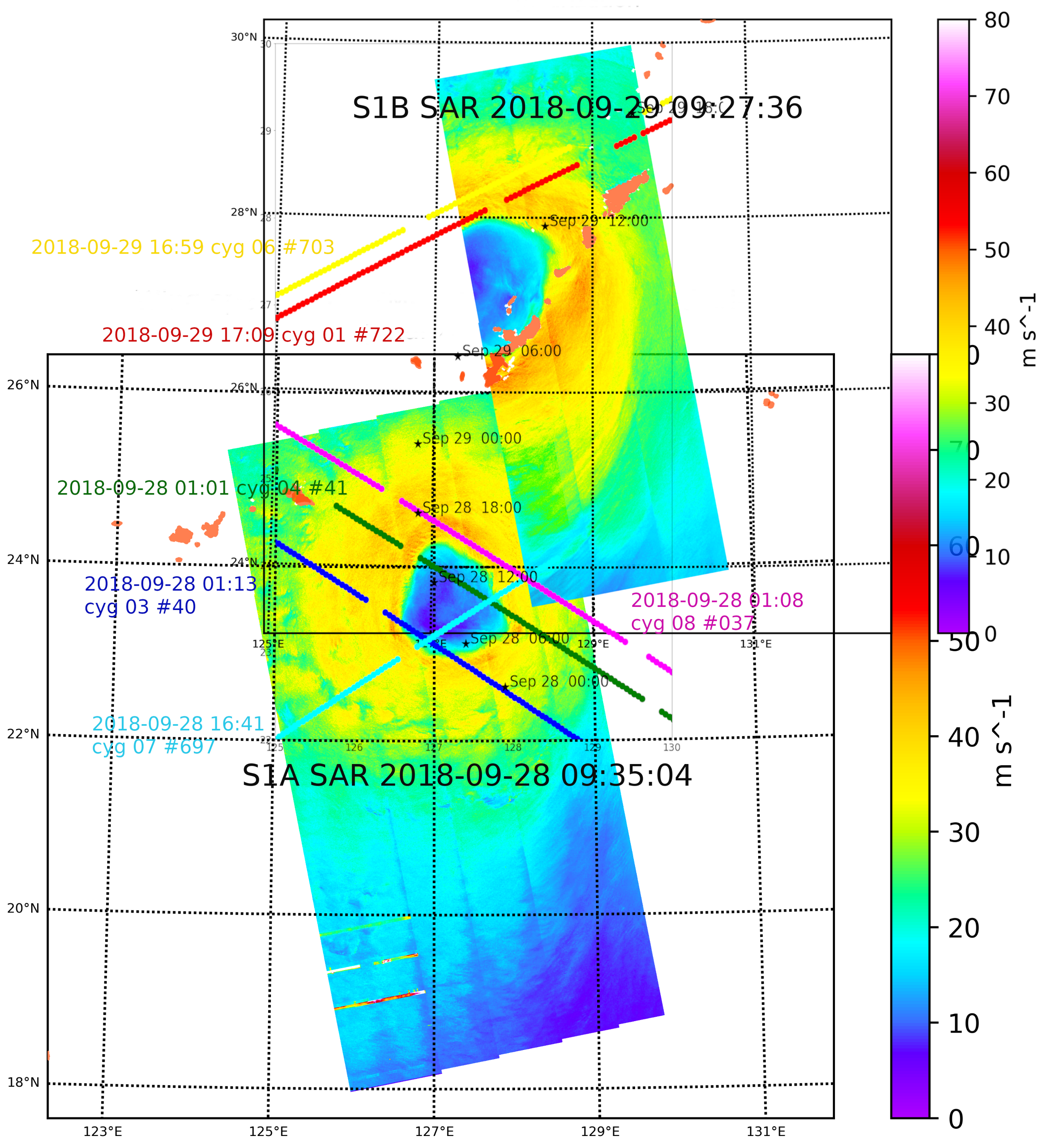
For illustrative purposes, Figure 1 shows examples of the retrievals across the typhoon Trami acquired on 29 September 2018 (category-2). The figure shows good agreement between the background model and the CyGNSS retrievals in the range up to ∼20 m/s, whereas CyGNSS results in higher winds at regions of strong winds. Furthermore, the eye of the cyclone is clearly captured by CyGNSS, proving the skills of the technique in order to capture rapid variations in the wind fields. The CyGNSS tracks across these examples do not show signs of saturation at high winds, reaching values above 40 m/s in some cases, similar to the Sentinel 1-B SAR wind retrievals that were obtained ∼8 h before.Figure A1, Appendix B displays the SAR wind retrieval images and CyGNSS tracks close to the hurricane eye. Both the range of wind speeds and shape of each track-slice are consistent with the SAR images, when considering their displacement in time, as indicated by the eye trajectory coordinates (also provided in Figure A1). Both of the tracks shown in Figure 1 occurred at close distance to each other and short time delay, presenting remarkable self-consistency. Appendix B shows more examples of CyGNSS tracks crossing Trami typhoon.
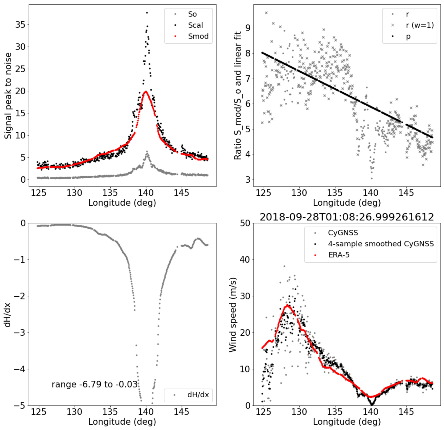
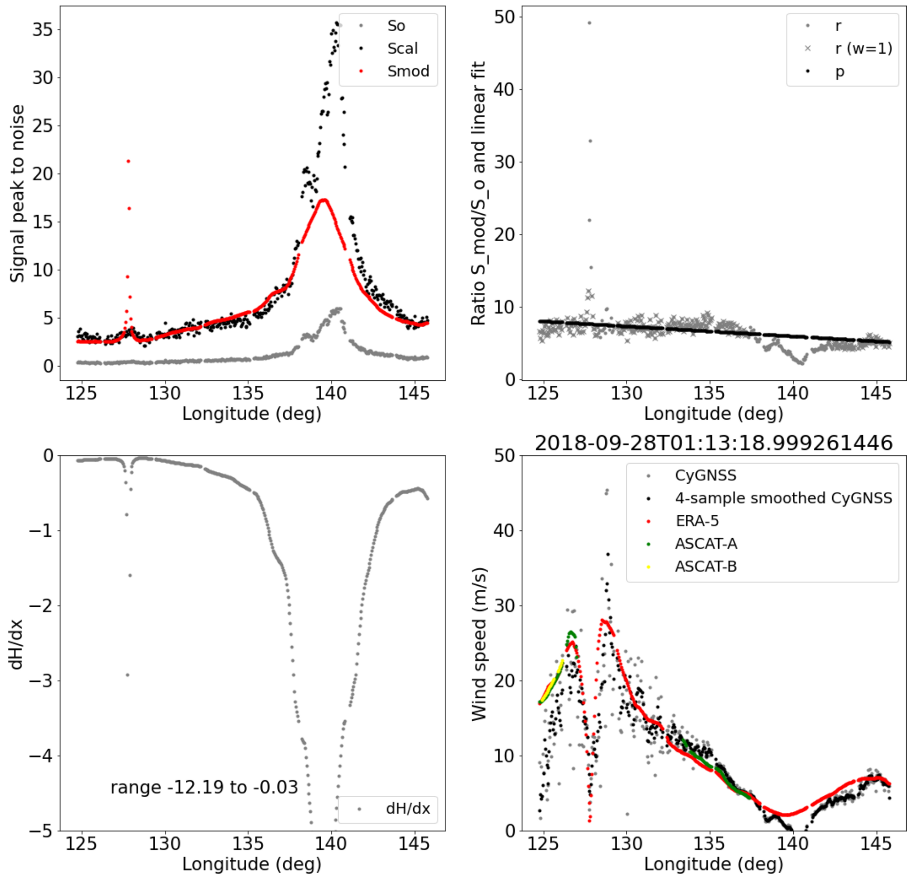
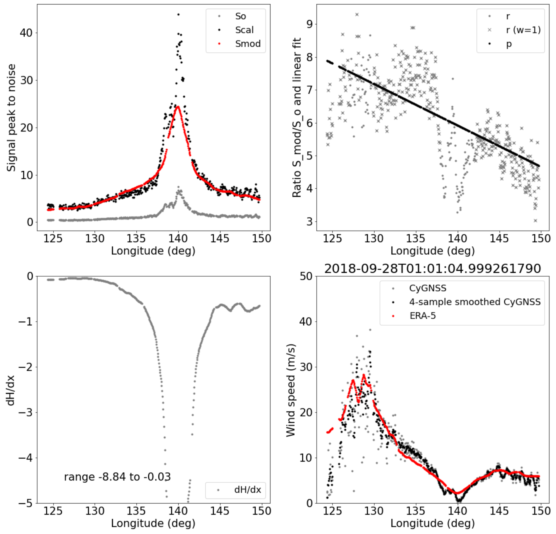
In order to illustrate the different intermediate parameters that are involved in the calibration and inversion of the data, Figure 2 shows, for these two tracks, the observed, modelled, and calibrated signal peak to noise S, the ratios r between the modelled and observed S m o d / S o together with the linear fit used for the calibration p, and the sensitivity H / x | x b . Appendix B also displays the intermediate parameters for the CyGNSS tracks crossing Trami typhoon during 28 September 2018.

3.2. Statistical Analysis: Comparison with the Background Model

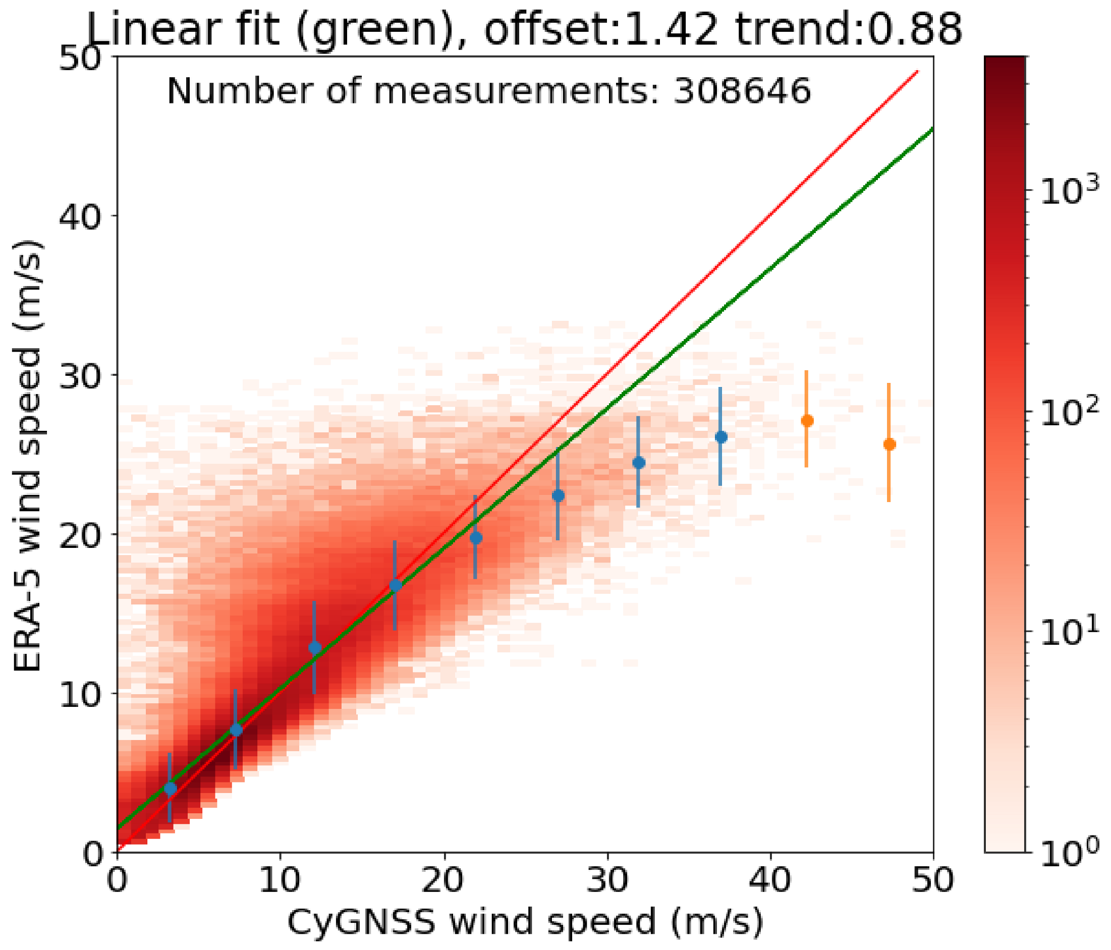
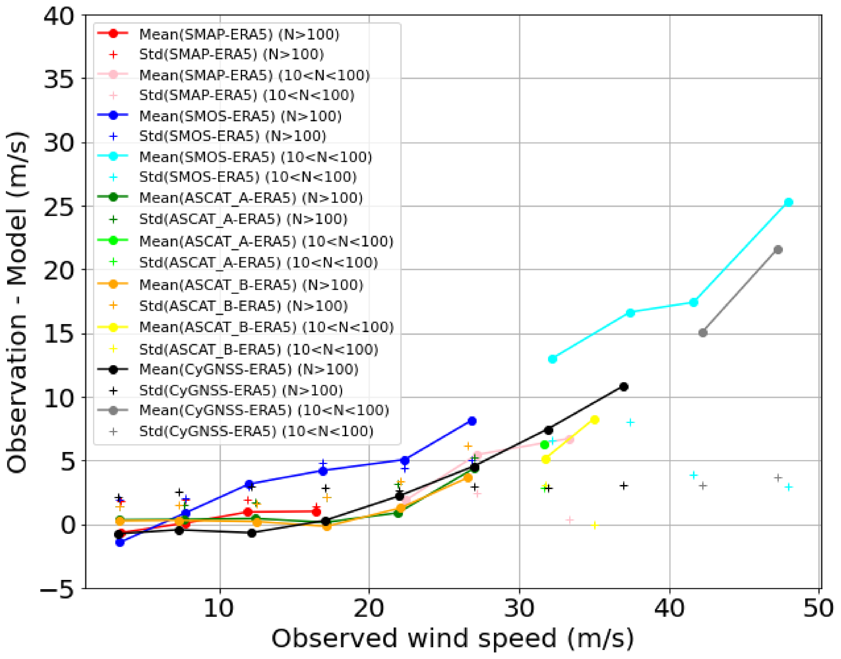
The examples that are provided in Figure 1 and Appendix B are not isolated cases: our CyGNSS retrievals generally match the background model at intermediate wind speeds well while also providing significantly higher winds for x b > 25  m/s. The Pearson’s correlation coefficient between both sets is 0.884. The statistics of the comparison with ERA5 wind values for the full set of analyzed data is displayed in the histogram of Figure 3 and the mean disagreement and dispersion in 5 m/s batches and for the whole set are compiled in Table 4. The saturation of the model at ∼30 m/s is clear in Figure 3, while CyGNSS can provide much higher wind speed values. Table 4 also shows the batched comparison between ERA5 and the other satellite measurements that are co-located with CyGNSS, and the values are graphically shown in Figure 4. The biases are defined as ‘observation minus background model’, with a positive bias indicating larger wind speed measurements than model values. This figure shows that our CyGNSS retrievals present biases with respect to the model that is very similar to the biases found for other spaceborne sensors, especially SMAP measurements, for which there are co-located values up to the range of 35-to-40 m/s wind speeds. At lower wind speeds, the CyGNSS-ERA5 statistics are also very similar to those of ASCAT-A and -B. The SMOS biases present a similar profile, but with an overall offset of a few m/s. All of these spaceborne wind measurements present higher biases at higher wind speeds, which is consistent with the fact that numerical weather prediction and re-analysis models tend to underestimate high wind speeds.

3.3. Statistical Analysis: Comparison with Other Spaceborne Sensors

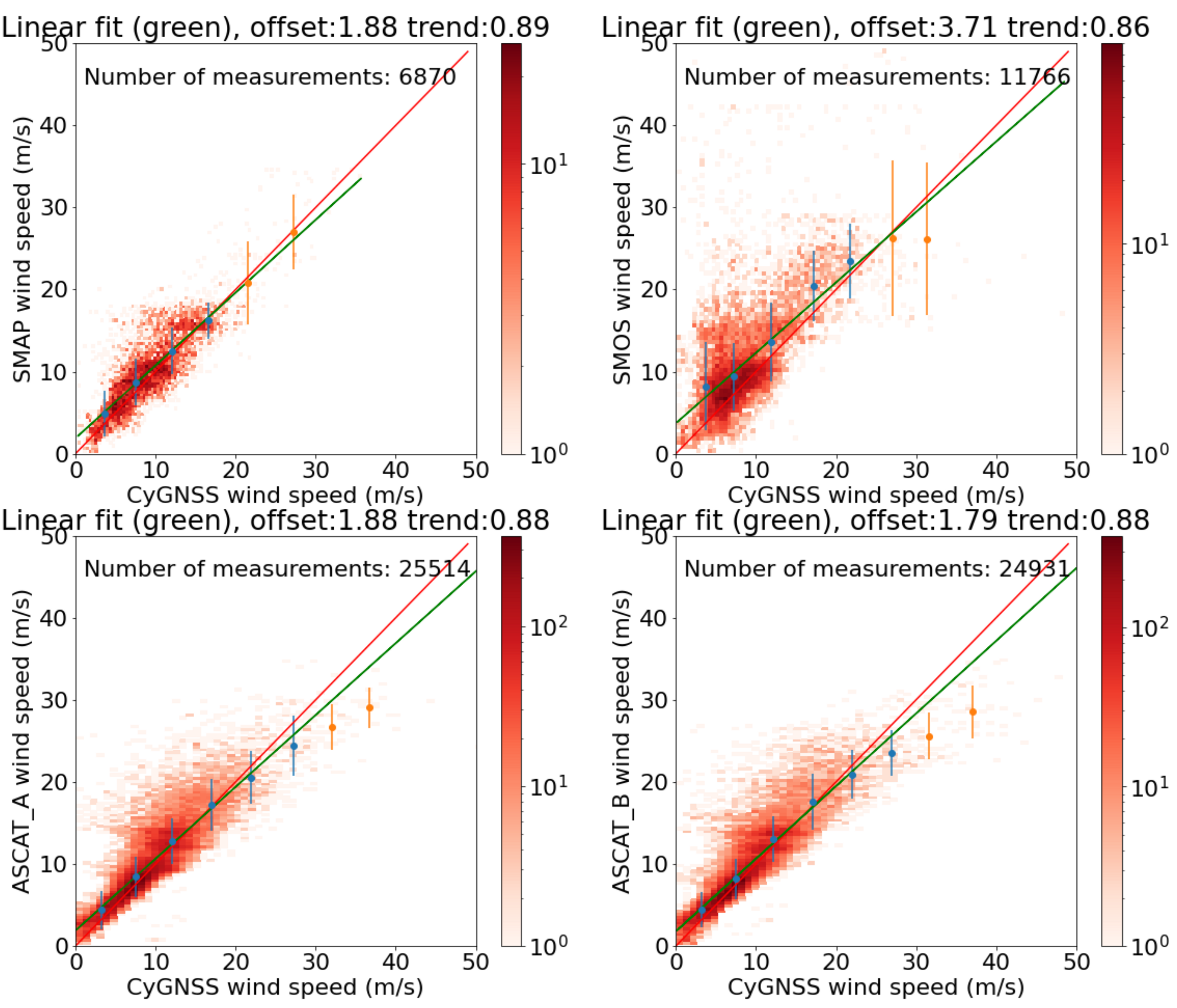
In this section, we present the direct comparison between our CyGNSS wind retrievals and the wind measurements obtained from other spaceborne sensors: the L-band radiometers SMAP and SMOS and the C-band wind scatterometers ASCAT-A and -B. Only wind measurements that were acquired within grid cells of 0.25 × 0.25 and 1 h time difference between CyGNSS and the other sensors have been considered (co-location criteria). The total numbers of available co-located measurements per sensor are compiled in Table 3. Figure 5 shows the histogram distribution of the correspondence between our CyGNSS wind retrievals and each of the other sensors. A linear fit is displayed in green, and its parameters are written on the top of each plot. The mean and dispersion within windows of 5 m/s are also shown with dots and errorbars, respectively. Table 5 summarizes the overall and batched comparisons.
Our CyGNSS retrievals agree well with SMAP wind measurements: the overall bias is −0.8 m/s, the linear fit is close to the 1:1 diagonal, and the 5-m/s batched means present differences that are between −1.2 to 1.8 m/s, with the latter at the range (35,40) m/s, thus better than 5% of the wind value. The dispersion between both spaceborne wind measurements is reasonable, with an overall standard deviation of 2.6 m/s and the dispersion in batches of 5 m/s below 3 m/s, except in the range (20,30) m/s, where it climbs up to ∼5 m/s dispersion. The Pearson’s correlation coefficient between SMAP and our CyGNSS wind products is relatively high (0.831). These are better values than the comparison with SMOS wind retrievals, which, in general, show much larger disperion (between 4.1 and 9.5 m/s).
Overall, the SMOS retrievals are significantly higher than our CyGNSS retrievals at low to moderate wind speeds, with −4.5 m/s bias between (0,5) m/s CyGNSS winds and 5.4 m/s dispersion. It is also possible to see a number of cases for which our CyGNSS inversion results in relatively low winds (<20 m/s), while SMOS obtains very strong winds (>40 m/s). The worse dispersion, with 9.5 m/s standard deviation, occurs at the range (25,30), where the bias is only 0.8 m/s. Nonetheless, these numbers are not statistically significant, given that there is less than 100 samples in that range of wind speeds (see orange dots/errorbars in Figure 5). The correlation coefficient between our and SMOS estimates is the lowest (0.646), and the overall bias and standard deviation is −2.5 and 4.6 m/s, respectively.
The comparison between our CyGNSS wind speed retrievals and those of ASCAT-A and -B are both similar, with ASCATs showing slight saturation around ∼30 m/s wind speed. They both present a correlation coefficient with our CyGNSS wind estimates close to 0.9 (0.862 for ASCAT-A and 0.881 for ASCAT-B). The overall bias is −0.8 m/s in both cases, with very similar dispersion values (2.4 and 2.5 m/s standard deviation, respectively).
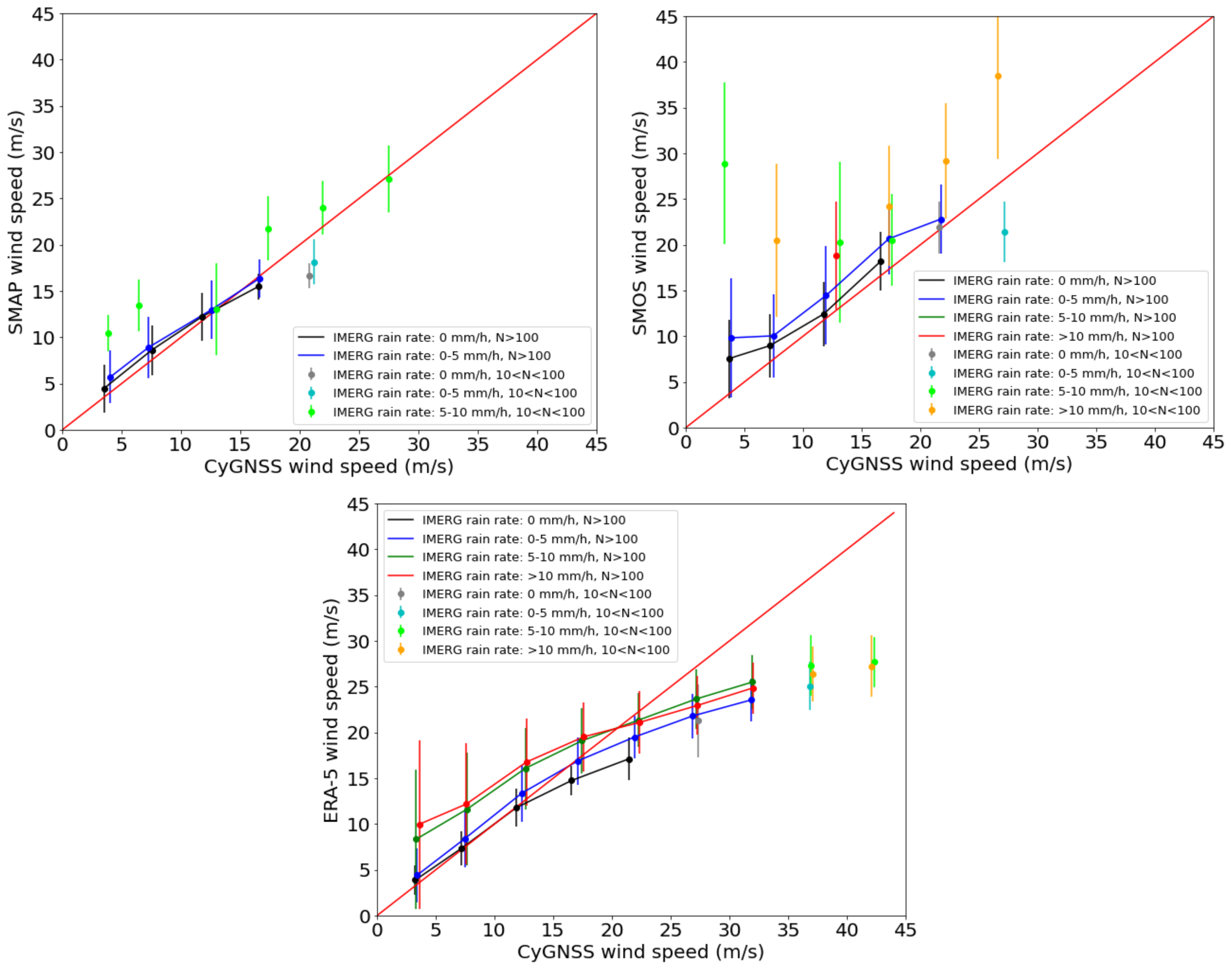
Any potential effects of the rain onto the CyGNSS measurements are first investigated while using the wind retrievals from the L-band radiometers SMAP and SMOS as reference, as it is claimed that these are unaffected or affected little by rain e.g., [44,45]. The reasons provided to justify minimal contamination by rain effects would similarly apply to CyGNSS GNSS-R measurement principle (i.e., little attenuation by rain droplets and small rain-induced roughness effects at L-band). The IMERG rain rate values that are co-located with CyGNSS measurements are used to bin the wind retrievals as a function of the rain rate. Figure 6 shows the batched means grouped by rain rate. Our variational CyGNSS wind retrievals show the same performance, within dispersion levels, as compared to SMAP and SMOS retrievals, regardless of the presence of rain up to 5 mm/h (heavy rain). The batches of co-locations with higher rain rates (heavy to violent showers) have been found to present a bias towards larger SMAP and SMOS wind retrievals, with larger biases for lower CyGNSS wind speeds. Nevertheless, none of the batches for rain rates above 5 mm/h present populations of statistically significant size (N < 100). For completeness, Figure 6-bottom shows the same rain-grouped statistics that were obtained for the comparison with ERA5. A similar residual effect that is linked to the presence of rain can be observed, with a larger impact on low wind speeds.

3.4. Statistical Analysis: Comparison with Other CyGNSS Wind Retrievals

The CyGNSS wind retrievals that are independently obtained by other organizations (see Section 2.1) are naturally co-located with our retrievals. The differences between our and other organizations’ CyGNSS retrievals are due to the inversion algorithms and the type and portion of observable used for extracting the geophysical information content. For example, the official CyGNSS products available at PODAAC use a larger part of the CyGNSS delay-Doppler map than our approach. This can slightly change the spatial resolution of the retrievals. Similarly, different quality flags and outliers might appear for each of these different retrieval algorithms; hence, the number of measurements available for each comparison can differ.
The GNSS-R observables are ultimately sensitive to a particular range of scales of the sea surface roughness (L-band roughness). These contributions to the sea surface spectra are induced by the wind, but also by other phenomena, like swell. Swell induces a small increase in the L-band roughness, which is usually only noticeable when the wind-driven roughness is mild (low winds regime). Even the wind contribution to the surface roughness can vary as function of the time passed since the wind started blowing and the size over which it blows (waves age and fetch, respectively). At the extremes, it is possible to define the Fully Developed Seas (FDS) and the Young Seas Limited Fetch (YSLF) regimes. Under FDS conditions, the input of energy to the waves from the local wind is in balance with the transfer of energy among the different wave components, and with the dissipation of energy by wave breaking, so the waves have reached their possible maximum height. By contrast, the waves are still building up in the YSLF regime. This is of particular interest at L-band measurements, as they are sensitive to relatively long roughness scales, which require more time to build up. Therefore, a moderate sea surface roughness, as measured by CyGNSS, can correspond to a moderate wind speed under FDS or a much higher wind speed under YSLF. The official CyGNSS products are independently generated while using two distinctive GMFs, one for each wave age regime. The user can then pick which assumption is more representative of the actual scenario (e.g., YSLF retrievals are recommended across tropical cyclones, because the YSLF GMF is determined while using match-ups between CyGNSS and airborne in-situ wind measurements across hurricanes).
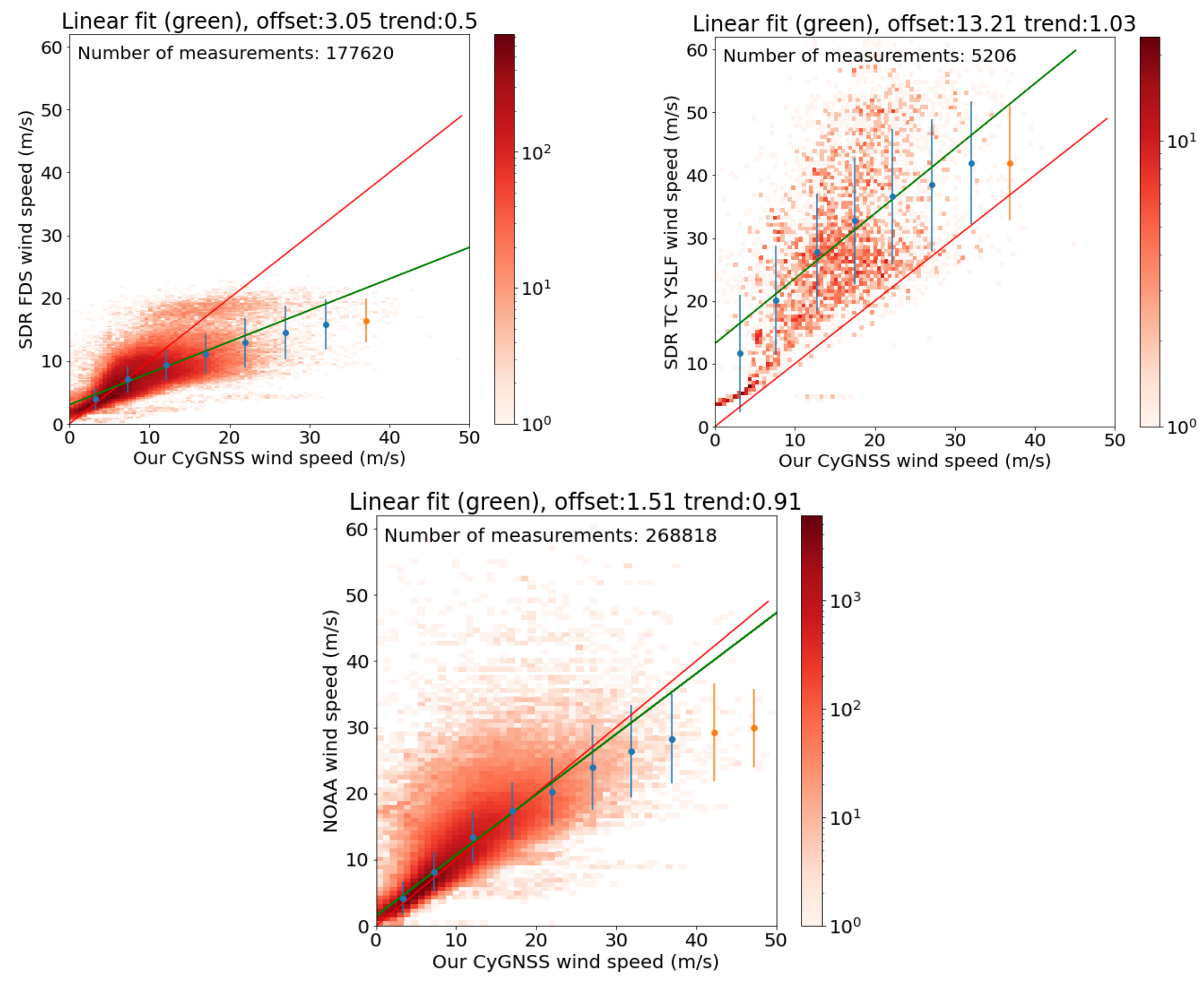
Figure 7 presents the 2D histograms of the correspondence between our and other organizations’ CyGNSS retrievals. The top row shows the comparison with the CyGNSS official SDR (version 3) wind speed when assuming fully developed seas (on the left) and young seas limited fetch (on the right). The YSLF plot has a much lower population, because we only present CyGNSS measurements occurring within 34 knots radius of the center of tropical cyclones. This flagging has been done comparing the CyGNSS specular points locations with the information that is provided in the ‘best track’ IBTrACS products [42]. These products have a 3 h sampling and, among other parameters, they list the center of the cyclone and four values of the 34 kn radius, one along each cardinal direction. We have averaged them to be four and checked that the CyGNSS distance to the eye is shorter than the averaged radius, within up to 1.5 h time offset from the record in IBTrACS. The spatial resolution our CyGNSS retrievals do not necessarily match those of other organizations’ retrievals, so this could add some dispersion level, as mentioned above.
The retrievals that are based on fully developed seas’ GMF present a clear saturation around ∼30 m/s wind, which is not present in our CyGNSS retrievals. Nevertheless, the Pearson’s correlation coefficient between our and SDR FDS CyGNSS wind retrievals is relatively high, 0.74. The saturation effect disappears when the young seas limited fetch GMF is used for the inversion, which results in very strong winds. The comparison between our CyGNSS solutions and the official SDR YSLF estimates present a very large bias, with SDR YSLF winds being higher than our estimates by nearly 14 m/s, even at low and moderate winds. The dispersion is also very large (9.9 m/s) and the Pearson’s correlation coefficient is relatively low (0.60).
The best correlation is found with NOAA CyGNSS wind retrievals (Figure 7-bottom), with a Pearson’s correlation coefficient of 0.832, which is very similar to the coefficient obtained with the SMAP L-band radiometer (0.831). The wind speed estimates that are obtained with NOAA’s and our algorithms agree very well in the range of winds up to 20 m/s. In this range, the histogram shows a tail towards NOAA larger winds, but this is not statistically significant (the figures use logaritmic color scale), and the batched means at these range of wind speeds sit along the 1:1 diagonal. Above 20 m/s, some tail persists (up to ∼30 m/s), but the means turn towards lower NOAA wind values.

4. Discussion

This study presented a variational retrieval algorithm in order to extract wind speed estimates from CyGNSS uncalibrated observables. The uniqueness of this approach can be summarized in the following points:
  • It uses uncalibrated observables obtained from a single pixel (the peak) of the signal-to-noise DDM, of slightly finer spatial resolution than the combination of pixels used in other CyGNSS retrieval approaches.
  • The retrieval is based on a physical forward model instead of empirical or semi-empirical GMF. The physical model has the potential to adjust to different parameters and scenarios, here reduced to wind speed solely. The other set of retrieval studies based on physical models used a large portion of the DDM [30,31,32], putting strong requirements on absolute and inter-pixel calibration, platform attitude control, and potential problems with delay-Doppler pixels that come from two cells on the surface (delay-Doppler ambiguity). For example, Huang et al. assessed that the assimilation of these DDM observables in hurricane models had to be restricted to ambiguity-free pixels [31].
  • The calibration is done with respect to a background model, ERA5 in our case. It consists of adjusting a polynomial (the linear trend obtained the best results) between the CyGNSS measured observables and those that result of feeding the forward model with ERA5 wind fields where it takes values between 5 and 25 m/s (to avoid the problems within the low wind regime in our physical model, and problems within strong winds in ERA5). Only long tracks of data are used to guarantee that wind anomalies (of shorter scale) can be separated from calibration issues (of much longer scale).
  • The retrieval scheme is compatible with a simplified example of the procedure of assimilation of low level observables in NWP models, in which the calibration could also be implemented. Therefore, the calibration would be consistent with the background model and independent from third parties’ NWP models (unlike assimilating CyGNSS retrievals calibrated with the data provider’s NWP model).
We anticipated that the approach would work at moderate wind speeds, but feared that the calibration against a background model would drag high wind retrievals towards the background values, i.e., underestimating the wind speed estimates. The comparison of the results to the ERA5 wind fields confirms the good performance in the range up to 20 m/s, with observation-background biases between −0.7 to 0.3 m/s and dispersion values between 2.2 and 3.0 m/s. These dispersion values could be improved by averaging subsequent samples (as can be visually checked in the black points of Figure 1 and Figure A2, Figure A3, Figure A4 and Figure A5). Above 20 m/s, the CyGNSS variational wind retrievals do not saturate, which presents an offset with respect to ERA5 that grows with the wind speed, thus confirming that the calibration approach does not constrain the wind retrievals towards the ERA5 underestimated values. The dispersion stays relatively low, with 3.7 m/s being the worst of them, in the range between 45 and 50 m/s (<8.5%). These offsets and dispersion values are similar to those that result from comparisons between ERA5 and other spaceborne sensors, such as the L-band radiometers SMOS and SMAP and the C-band scatterometers ASCAT-A/B.
When the variational CyGNSS retrievals are directly compared against co-located measurements by these spaceborne L-band and C-band sensors, the best agreement is found with the ASCAT A/B scatterometers (nearly 0.9 correlation coefficient). The comparison with SMAP, also with high Pearson’s correlation coefficient (0.831), is consistent, regardless of the rain, up to 5 mm/h rain rate (heavy rain). Above 5 mm/h (heavy and violent showers), SMAP presents slightly higher wind values. This could be an effect on the CyGNSS side (underestimation of wind under intense rain) or an effect on the SMAP side (overestimation of the wind under intense rain). In principle, rain would not underestimate the GNSS-R retrievals, as all rain-related effects would push the observables towards those that correspond to higher wind scenarios: lower received reflected power by increased atmospheric attenuation and rain-splash induced roughness. The same conclusion was reached in [50] through simulations, where it was stated that rain scenarios would overestimate the GNSS-R wind retrievals. A possible explanation to what is found here could be the rain-induced modulation of the long surface wavelengths (L-band sensitive waves), flattening, or smoothing them e.g., [51]. However, it seems that this would also affect the L-band emissivity in the same way, unless, e.g., foam effects in L-band emissivity at high winds prevail to the flattening one. This effect is stronger in comparison with SMOS, particularly at low CyGNSS-retrieved winds. Similar effects are seen in the comparison with ERA5, with more robust statistics. However, [52] showed that TDS-1 bistatic radar cross section was sensitive to rain at wind speeds of below 6 m/s, insensitive at higher wind speeds, and the sensitivity was in the opposite sense of our finding: the rain scenarios presented lower cross section than rain-free cases, thus it would have been inverted into higher winds. According to that study, the GNSS-R observables do not explain the results that we have found. This open interesting questions: (1) do NWP models overestimate wind speeds in presence of intense rain? (for example, due to the assimilation of higher frequency-band scatterometer measurements, which do have positive bias especially at low wind regimes e.g., [53]); (2) is the single-pixel observable used in our study sensitive to the rain smoothing effect, but this is lost when the received power is averaged across a wider area of the DDM (as the observables used in [52])? Further studies would be required to answer these questions.
The CyGNSS retrievals have also been compared to those that are produced by other organizations, based on different algorithms. The best agreement is found with NOAA’s retrievals, with 0.832 Pearson’s correlation coefficient. It would be interesting to check whether the differences come from the algorithm itself or from the fact that our implementation and NOAA’s use a different background model. The lowest correlation is found between our retrievals and the official products that are obtained with the YSLF assumption, with a very large overall bias (−13.8 m/s, SDR YSLF retrievals higher than ours) and dispersion (9.9 m/s), even at low and moderate wind speeds.
In conclusion, this approach has shown skills for inferring a broad range of wind speeds, including hurricane force winds, from uncalibrated bin raw counts of CyGNSS level-1 observables, coming from the peak-pixel and based on physical forward models. The variational retrieval algorithm is a simplified version of the more general equations that are used in data assimilation, and the calibration scheme could also be integrated in the assimilation process. Therefore, this approach is also a good tool for analyzing the potential performance of ingesting level-1 single-pixel observables into NWP. For example, the statistics of the differences between observations and background model (O-B) are similar to those of ASCAT-A/B, SMOS, and SMAP, some of which are already successfully assimilated into weather prediction models e.g., [54,55]. Furthermore, being based on a physical forward model, which is ultimately fed by a wind-wave spectrum, the data assimilation scheme could expand beyond wind speed to use the ruling parameters of the spectrum. While this might not be feasible in the form of variational retrievals (under-determined system or strongly correlated unknowns), the over-determination and ancillary information embedded in numerical models would potentially enable these expanded uses in data assimilation schemes, with the added value of consistently calibrating the observables with the background model.

Author Contributions

Conceptualization, A.R. and E.C.; methodology, A.R.; software, A.R. and E.C.; validation, E.C.; formal analysis, E.C.; investigation, A.R. ; data curation, A.R., Y.N. and R.P.; writing—original draft preparation, E.C.; writing—review and editing, E.C., A.R., W.L. and S.R.; visualization, E.C.; supervision, A.R.; project administration, E.C.; funding acquisition, E.C. All authors have read and agreed to the published version of the manuscript.

Funding

This research was funded by the Spanish Ministry of Science, Innovation and Universities grant number RTI2018-099008-B-C22/AEI/10.13039/501100011033/FEDER, EU, with computing facilities covered by grant EQC2019-005664-P. Yang NAN appreciated the financial support from China Scholarship Council (CSC) by a State Scholarship Fund (No.201906270212). This investigation is done in the frame of the NASA CyGNSS Extended Science Team and it represents a contribution to CSIC Thematic Interdisciplinary Platform PTI TELEDETECT. Part of this study is a contribution to ESA C.N.4000132954/20/I-NB.

Conflicts of Interest

The authors declare no conflict of interest. The funders had no role in the design of the study; in the collection, analyses, or interpretation of data; in the writing of the manuscript, or in the decision to publish the results.

Abbreviations

The following abbreviations are used in this manuscript:
ASCATEUMETSAT Advanced Scatterometer on board METOP
CDRCYGNSS Climate Data Record
CLSCollecte Localisation Satellites, France
CYGNSSNASA Cyclone Global Navigation Satellite System
DDMDelay Doppler Map
ECMWFEuropean Centre for Medium-range Weather Forecast
ERA5ECMWF Reanalysis 5th Generation
ECMWF/C3SECMWF/Copernicus Climate Change Service
FDSFully Developed Seas
GMFGeophysical Model Functions
GNSSGlobal Navigation Satellite System
GNSS-RGNSS Reflectometry
GPSUSA Global Positioning System
IBTrACSInternational Best Track Archive for Climate Stewardship
IFREMERInstitut Français de Recherche pour l’Exploitation de la Mer
IMERGIntegrated Multi-satellitE Retrievals for Global Precipitation Measurement (GPM) mission
L1X21CYGNSS Level 1 Science Data Record Version 2.1
LEOLow Earth Orbiter
MEBEXMediterranean Balloon Experiment
NASAUSA National Aeronautics and Space Administration
NOAAUSA National Oceanic and Atmospheric Administration
NWPNumerical Weather Prediction
PODAACNASA’s Physical Oceanography Distributed Active Archive Center
SARSynthetic Aperture Radar
SFMRNOAA Stepped Frequency Microwave Radiometer
SMAPNASA Soil Moisture Active Passive
SMOSESA Soil Moisture and Ocean Salinity
TDS-1UK TechDemoSat-1
YSLFYoung Seas Limited Fetch

Appendix A. Symbols in Section 2.2

The symbols used in Section 2.2 are compiled in Table A1.
Table A1. Symbols used in Section 2.2.
SymbolDescriptionIn This Study
y o Generic symbol for the observable being assimilated or inverted S o c a l
xGeneric symbol for the unknowns to be retrievedwind speed
x b Values of the unknowns according to the background modelERA5 u 10 2 + v 10 2
HForward model or operator to synthesize a simulated observable from a model that depends on xBistatic radar equation for GNSS in [2] as implemented in ‘wavpy’ [48]
BCovariance matrix of the background modelnot used
ECovariance matrix of the measurementsIdentity matrix
FCovariance matrix of the forward operatornot used
SGeneric symbol for signal peak to noise level m a x ( D D M ) / f l o o r ( D D M ) 1
S m o d S modelled using the forward operator fed with the background model S m o d = H [ x b ]
S o S extracted from CyGNSS level-1 data m a x ( D D M o ) / f l o o r ( D D M o ) 1 with D D M o variable raw_counts ‘DDM bin raw counts’
S o c a l S o after the calibration step S o c a l = p S o
pPolynomial fit of the ratios rliner fit better performance
rinverse ratio between a given observation and its modelled value r = S m o d / S o
H x | x b Derivative or the forward operator with respect to the unknowns, evaluated at x b Numerical derivative

Appendix B. Trami Figures

The CyGNSS tracks shown in Figure 1 and Figure 2 crossed Trami typhoon in 29 September 2018, approximately ∼8 h after Sentinel-1B overpassed the area. The SAR-derived winds, obtained from Ifremer/Cyclobs e.g., [46] are shown in Figure A1 together with these two CyGNSS tracks (in red and yellow). Nearly 24 h before, on 28 September 2018, Sentinel-1A also overpassed the area, capturing another SAR-derived image, approximately ∼8 h after CyGNSS had acquired the tracks in pink, green and blue, and ∼7 h before the cyan track. At these time intervals, the eye of the cyclone translated across the area, as shown in black stars. The intermediate parameters and final solutions for these set of CyGNSS tracks are displayed in Figure A2, Figure A3, Figure A4 and Figure A5.
Figure A1. Sentinel-1A and -1B wind retrievals for Typhoon ‘Trami’, acquired on 28 September 9:35 (lower) and 29 September 9:27 (upper) 2018, approximately 24 h apart. The CyGNSS tracks crossing the hurricane close to its eye are displayed in different colors, together with the acquisition time-stamp of one of their samples. The red and yellow tracks correspond to the left and right plots in Figure 1, respectively. The rest of colours correspond to the examples provided in Figure A2, Figure A3, Figure A4 and Figure A5. The black stars and time labels correspond to the eye trajectory at 6 h sampling. The SAR wind product images were obtained from Ifremer/Cyclobs, produced with a SAR wind processor co-developped by IFREMER and CLS e.g., [46].
Remotesensing 12 03930 g0a1
Figure A2. Intermediate parameters and final wind retrievals for CyGNSS satellite 08, track number 37, magenta track in Figure A1. (Top-left): S o , S m o d and S o c a l . (Top-right): Ratios r and fit p. (Bottom-left): Sensitivity H / x | x b . (Bottom-right): 1 Hz wind retrievals, 0.25 Hz smoothed solution, and ERA5 wind estimate.
Remotesensing 12 03930 g0a2
Figure A3. Same as Figure A2 for CyGNSS satellite 03, track number 40, blue track in Figure A1. Co-locations with ASCAT-A/B were also found (bottom-right panel).
Remotesensing 12 03930 g0a3
Figure A4. Same as Figure A2 for CyGNSS satellite 04, track number 41, green track in Figure A1.
Remotesensing 12 03930 g0a4
Figure A5. Same as Figure A2 for CyGNSS satellite 07, track number 697, cyan track in Figure A1.
Remotesensing 12 03930 g0a5

References

  1. Ruf, C.S.; Atlas, R.; Chang, P.S.; Clarizia, M.P.; Garrison, J.L.; Gleason, S.; Katzberg, S.J.; Jelenak, Z.; Johnson, J.T.; Majumdar, S.J.; et al. New ocean winds satellite mission to probe hurricanes and tropical convection. Bull. Am. Meteorol. Soc. 2016, 97, 385–395. [Google Scholar] [CrossRef]
  2. Zavorotny, V.U.; Voronovich, A.G. Scattering of GPS signals from the ocean with wind remote sensing application. IEEE Trans. Geosci. Remote. Sens. 2000, 38, 951–964. [Google Scholar] [CrossRef] [Green Version]
  3. Zavorotny, V.U.; Gleason, S.; Cardellach, E.; Camps, A. Tutorial on Remote Sensing Using GNSS Bistatic Radar of Opportunity. IEEE Geosci. Remote. Sens. Mag. 2014, 2, 8–45. [Google Scholar] [CrossRef] [Green Version]
  4. Jin, S.; Cardellach, E.; Xie, F. GNSS Remote Sensing: Theory, Methods and Applications; Springer: Dordrecht, The Netherlands, 2014; ISBN 978-94-007-7481-0. [Google Scholar] [CrossRef]
  5. Rius, A.; Cardellach, E. Reflectometry. In Springer Handbook of Global Navigation Satellite Systems; Teunissen, P., Montenbruck, O., Eds.; Springer International Publishing: Cham, Switzerland, 2017; pp. 1163–1186. ISBN 978-3-319-42928-1. [Google Scholar] [CrossRef]
  6. Katzberg, S.J.; Walker, R.A.; Roles, J.H.; Lynch, T.; Black, P.G. First GPS signals reflected from the interior of a tropical storm: Preliminary results from Hurricane Michael. Geophys. Res. Lett. 2001, 28, 1981–1984. [Google Scholar] [CrossRef] [Green Version]
  7. Cardellach, E.; Ruffini, G.; Pino, D.; Rius, A.; Komjathy, A.; Garrison, J.L. Mediterranean Balloon Experiment: Ocean wind speed sensing from the stratosphere using GPS reflections. Remote. Sens. Environ. 2003, 88, 351–362. [Google Scholar] [CrossRef]
  8. Clarizia, M.P.; Ruf, C.; Cipollini, P.; Zuffada, C. First spaceborne observation of sea surface height using GPS-reflectometry. Geophys. Res. Lett. 2016, 43, 767–774. [Google Scholar] [CrossRef] [Green Version]
  9. Cardellach, E.; Li, W.; Rius, A.; Semmling, M.; Wickert, J.; Zus, F.; Ruf, C.; Buontempo, C. First Precise Spaceborne Sea Surface Altimetry With GNSS Reflected Signals. IEEE J. Sel. Top. Appl. Earth Obs. Remote Sens. 2020, 13, 102–112. [Google Scholar] [CrossRef]
  10. Li, W.; Cardellach, E.; Fabra, F.; Rius, A.; Ribó, S.; Martín-Neira, M. First spaceborne phase altimetry over sea ice using TechDemoSat-1 GNSS-R signals. Geophys. Res. Lett. 2017, 44, 8369–8376. [Google Scholar] [CrossRef]
  11. Rius, A.; Cardellach, E.; Fabra, F.; Li, W.; Ribó, S.; Hernández-Pajares, M. Feasibility of GNSS-R Ice Sheet Altimetry in Greenland Using TDS-1. Remote. Sens. 2017, 9, 742. [Google Scholar] [CrossRef] [Green Version]
  12. Cartwright, R.; Banks, C.J.; Srokosz, M. Improved GNSS-R bi-static altimetry and independent digital elevation models of Greenland and Antarctica from TechDemoSat-1. Cryosphere 2020, 14, 1909–1917. [Google Scholar] [CrossRef]
  13. Li, W.; Cardellach, E.; Fabra, F.; Ribó, S.; Rius, A. Lake Level and Surface Topography Measured With Spaceborne GNSS-Reflectometry From CYGNSS Mission: Example for the Lake Qinghai. Geophys. Res. Lett. 2018, 45, 13332–13341. [Google Scholar] [CrossRef]
  14. Yan, Q.; Huang, W. Spaceborne GNSS-R Sea Ice Detection Using Delay-Doppler Maps: First Results From the U.K. TechDemoSat-1 Mission. IEEE J. Sel. Top. Appl. Earth Obs. Remote. Sens. 2016, 9, 4795–4801. [Google Scholar] [CrossRef]
  15. Alonso-Arroyo, A.; Zavorotny, V.U.; Camps, A. Sea Ice Detection Using U.K. TDS-1 GNSS-R Data. IEEE Trans. Geosci. Remote Sens. 2017, 55, 4989–5001. [Google Scholar] [CrossRef] [Green Version]
  16. Li, W.; Cardellach, E.; Fabra, F.; Ribó, S.; Rius, A. Measuring Greenland Ice Sheet Melt Using Spaceborne GNSS Reflectometry From TechDemoSat-1. Geophys. Res. Lett. 2020, 47. [Google Scholar] [CrossRef]
  17. Chew, C.; Shah, R.; Zuffada, C.; Hajj, G.; Masters, D.; Mannucci, A.J. Demonstrating soil moisture remote sensing with observations from the UK TechDemoSat-1 satellite mission. Geophys. Res. Lett. 2016, 43, 3317–3324. [Google Scholar] [CrossRef] [Green Version]
  18. Santi, E.; Paloscia, S.; Pettinato, S.; Fontanelli, G.; Clarizia, M.P.; Comite, D.; Dente, L.; Guerriero, L.; Pierdicca, N.; Floury, N. Remote Sensing of Forest Biomass Using GNSS Reflectometry. IEEE J. Sel. Top. Appl. Earth Obs. Remote Sens. 2020, 13, 2351–2368. [Google Scholar] [CrossRef]
  19. Rodriguez-Alvarez, N.; Podest, E.; Jensen, K.; McDonald, K.C. Classifying Inundation in a Tropical Wetlands Complex with GNSS-R. Remote Sens. 2019, 11, 1053. [Google Scholar] [CrossRef] [Green Version]
  20. Comite, D.; Cenci, L.; Colliander, A.; Pierdicca, N. Monitoring Freeze-Thaw State by Means of GNSS Reflectometry: An Analysis of TechDemoSat-1 Data. IEEE J. Sel. Top. Appl. Earth Obs. Remote Sens. 2020, 13, 2996–3005. [Google Scholar] [CrossRef]
  21. Unwin, M.; Jales, P.; Tye, J.; Gommenginger, C.; Foti, G.; Rosello, J. Spaceborne GNSS-Reflectometry on TechDemoSat-1: Early Mission Operations and Exploitation. IEEE J. Sel. Top. Appl. Earth Obs. Remote. Sens. 2016, 9, 4525–4539. [Google Scholar] [CrossRef]
  22. Foti, G.; Gommenginger, C.; Jales, P.; Unwin, M.; Shaw, A.; Robertson, C.; Roselló, J. Spaceborne GNSS reflectometry for ocean winds: First results from the UK TechDemoSat-1 mission. Geophys. Res. Lett. 2015, 42, 5435–5441. [Google Scholar] [CrossRef] [Green Version]
  23. Foti, G.; Gommenginger, C.; Srokosz, M. First Spaceborne GNSS-Reflectometry Observations of Hurricanes From the UK TechDemoSat-1 Mission. Geophys. Res. Lett. 2017, 44, 12358–12366. [Google Scholar] [CrossRef] [Green Version]
  24. Foti, G.; Gommenginger, C.; Unwin, M.; Jales, P.; Tye, J.; Rosello, J. An Assessment of Non-geophysical Effects in Spaceborne GNSS Reflectometry Data From the UK TechDemoSat-1 Mission. IEEE J. Sel. Top. Appl. Earth Obs. Remote. Sens. 2017, 10, 3418–3429. [Google Scholar] [CrossRef] [Green Version]
  25. Said, F.; Jelenak, Z.; Chang, P.S.; Soisuvarn, S. An Assessment of CYGNSS Normalized Bistatic Radar Cross Section Calibration. IEEE J. Sel. Top. Appl. Earth Obs. Remote. Sens. 2019, 12, 50–65. [Google Scholar] [CrossRef]
  26. Ruf, C.S.; Balasubramaniam, R. Development of the CYGNSS Geophysical Model Function for Wind Speed. IEEE J. Sel. Top. Appl. Earth Obs. Remote. Sens. 2019, 12, 66–77. [Google Scholar] [CrossRef]
  27. Ruf, C.S.; Gleason, S.; McKague, D.S. Assessment of CYGNSS Wind Speed Retrieval Uncertainty. IEEE J. Sel. Top. Appl. Earth Obs. Remote. Sens. 2019, 12, 87–97. [Google Scholar] [CrossRef]
  28. Ruf, C.; Asharaf, S.; Balasubramaniam, R.; Gleason, S.; Lang, T.; McKague, D.; Twigg, D.; Waliser, D. In-Orbit Performance of the Constellation of CYGNSS Hurricane Satellites. Bull. Am. Meteorol. Soc. 2019, 100, 2009–2023. [Google Scholar] [CrossRef]
  29. Said, F.; Jelenak, Z.; Park, J.; Soisuvarn, S.; Chang, P.S. A ‘Track-Wise’ Wind Retrieval Algorithm for the CYGNSS Mission. In Proceedings of the IGARSS 2019—2019 IEEE International Geoscience and Remote Sensing Symposium, Yokohama, Japan, 28 July–2 August 2019; pp. 8711–8714. [Google Scholar] [CrossRef]
  30. Huang, F.; Garrison, J.L.; Rodriguez-Alvarez, N.; O’Brien, A.J.; Schoenfeldt, K.M.; Ho, S.C.; Zhang, H. Sequential Processing of GNSS-R Delay-Doppler Maps to Estimate the Ocean Surface Wind Field. IEEE Trans. Geosci. Remote Sens. 2019, 57, 10202–10217. [Google Scholar] [CrossRef]
  31. Huang, F.; Grieco, G.; Stoffelen, A.; GNSS-R Processing and NWP Assimilation. EUMETSAT OSI SAF Visiting Scientist Activity Scientific Report V.1 2019. Available online: http://www.osi-saf.org/sites/default/files/dynamic/page_with_files/file/osisaf_vs19_01_Huang_Report_v1.0.pdf (accessed on 30 November 2020).
  32. Huang, F.; Garrison, J.L.; Leidner, S.M.; Annane, B.; Hoffman, R.N.; Grieco, G.; Stoffelen, A. A Forward Model for Data Assimilation of GNSS Ocean Reflectometry Delay-Doppler Maps. IEEE Trans. Geosci. Remote. Sens. 2020, 1–14. [Google Scholar] [CrossRef]
  33. Al-Khaldi, M.M.; Johnson, J.T.; Kang, Y.; Katzberg, S.J.; Bringer, A.; Kubatko, E.; Wood, D. Track-Based Cyclone Maximum Wind Retrievals Using the Cyclone Global Navigation Satellite System (CYGNSS) Mission Full DDMs. IEEE J. Sel. Top. Appl. Earth Obs. Remote. Sens. 2020, 13. [Google Scholar] [CrossRef]
  34. Li, M.; Liu, J.; Wang, Z.; Wang, H.; Zhang, Z.; Zhang, L.; Yang, Q. Assessment of Sea Surface Wind from NWP Reanalyses and Satellites in the Southern Ocean. J. Atmos. Oceanic Technol. 2013, 30, 1842–1853. [Google Scholar] [CrossRef]
  35. Whelan, E.; Gleeson, E.; Hanley, J. An Evaluation of MÉRA, a High-Resolution Mesoscale Regional Reanalysis. J. Appl. Meteorol. Climatol. 2018, 57, 2179–2196. [Google Scholar] [CrossRef]
  36. McNoldy, B.; Annane, B.; Majumdar, S.; Delgado, J.; Bucci, L.; Atlas, R. Impact of Assimilating CYGNSS Data on Tropical Cyclone Analyses and Forecasts in a Regional OSSE Framework. Mar. Technol. Soc. J. 2017, 51, 7–15. [Google Scholar] [CrossRef]
  37. Annane, B.; McNoldy, B.; Leidner, S.M.; Hoffman, R.; Atlas, R.; Majumdar, S.J. A Study of the HWRF Analysis and Forecast Impact of Realistically Simulated CYGNSS Observations Assimilated as Scalar Wind Speeds and as VAM Wind Vectors. Mon. Weather. Rev. 2018, 146, 2221–2236. [Google Scholar] [CrossRef]
  38. Li, X.; Mecikalski, J.R.; Lang, T.J. A Study on Assimilation of CYGNSS Wind Speed Data for Tropical Convection during 2018 January MJO. Remote Sens. 2020, 12, 1243. [Google Scholar] [CrossRef] [Green Version]
  39. Cotton, J.; Eyre, J.; Forsythe, M. Evaluation of TDS-1 winds in Numerical Weather Prediction. In GNSS-R Workshop; NOC Southampton: Southampton, UK, 2018; Available online: Http://merrbys.co.uk/wpcontent/uploads/2018/07/NOCWorkshop_JCotton_201805_share.pdf (accessed on 30 November 2020).
  40. University of Michigan. CYGNSS Handbook; Michigan Publishing: Ann Arbor, MI, USA, 2016; ISBN 978-1-60785-380-0. Available online: https://clasp-research.engin.umich.edu/missions/cygnss/reference/cygnss-mission/CYGNSS_Handbook_April2016.pdf (accessed on 30 November 2020).
  41. European Centre for Medium-range Weather Forecast (ECMWF) Copernicus Climate Change (C3S). ERA5: Fifth Generation of ECMWF Atmospheric Reanalyses of the Global Climate. On-Line Documentation, Last Version August 5. 2020. Available online: Https://confluence.ecmwf.int/display/CKB/ERA5%3A+data+documentation (accessed on 30 November 2020).
  42. Knapp, K.R.; Kruk, M.C.; Levinson, D.H.; Diamond, H.J.; Neumann, C.J. The International Best Track Archive for Climate Stewardship (IBTrACS): Unifying tropical cyclone best track data. Bull. Am. Meteorol. Soc. 2010, 91, 363–376. [Google Scholar] [CrossRef]
  43. Verspeek, J.A.; Stoffelen, A.; Portabella, M.; Bonekamp, H.; Anderson, C.; Figa, J. Validation and calibration of ASCAT using CMOD5.n. IEEE Trans. Geosci. Remote Sens. 2010, 48, 386–395. [Google Scholar] [CrossRef]
  44. Reul, N.; Tenerelli, J.; Chapron, B.; Vandemark, D.; Quilfen, Y.; Kerr, Y. SMOS satellite L-band radiometer: A new capability for ocean surface remote sensing in hurricanes. J. Geophys. Res. 2012, 117, C02006. [Google Scholar] [CrossRef] [Green Version]
  45. Meissner, T.; Ricciardulli, L.; Wentz, F.J. Capability of the SMAP Mission to Measure Ocean Surface Winds in Storms. Bull. Am. Meteorol. Soc. 2017, 98, 1660–1677. [Google Scholar] [CrossRef]
  46. Mouche, A.; Chapron, B.; Knaff, J.; Zhao, Y.; Zhang, B.; Combot, C. Copolarized and Cross-Polarized SAR Measurements for High-Resolution Description of Major Hurricane Wind Structures: Application to Irma Category 5 Hurricane. J. Geophys. Res. Ocean. 2019, 124, 3905–3922. [Google Scholar] [CrossRef]
  47. Huffman, G.J.; Stocker, E.F.; Bolvin, D.T.; Nelkin, E.J.; Tan, J. GPM IMERG Final Precipitation L3 Half Hourly 0.1 Degree × 0.1 Degree V06; Goddard Earth Sciences Data and Information Services Center (GES DISC): Greenbelt, MD, USA, 2019. [Google Scholar] [CrossRef]
  48. Fabra, F.; Cardellach, E.; Li, W.; Rius, A. WAVPY: A GNSS-R open source software library for data analysis and simulation. In Proceedings of the IGARSS 2017—IEEE International Geoscience and Remote Sensing Symposium, Fort Worth, TX, USA, 23–28 July 2017; pp. 4125–4128. [Google Scholar] [CrossRef]
  49. Voronovich, A.G.; Zavorotny, V.U. Bistatic Radar Equation for Signals of Opportunity Revisited. IEEE Trans. Geosci. Remote Sens. 2018, 56, 1959–1968. [Google Scholar] [CrossRef]
  50. Asgarimehr, M.; Wickert, J.; Reich, S. Evaluating Impact of Rain Attenuation on Space-borne GNSS Reflectometry Wind Speeds. Remote Sens. 2019, 11, 1048. [Google Scholar] [CrossRef] [Green Version]
  51. Laxague, N.J.M.; Zappa, C.J. The impact of rain on ocean surface waves and currents. Geophys. Res. Lett. 2020, 47, e2020GL087287. [Google Scholar] [CrossRef] [Green Version]
  52. Asgarimehr, M.; Zavorotny, V.; Wickert, J.; Reich, S. Can GNSS Reflectometry detect precipitation over oceans? Geophys. Res. Lett. 2018, 45, 12585–12592. [Google Scholar] [CrossRef] [Green Version]
  53. Portabella, M.; Stoffelen, A.; Lin, W.; Turiel, A.; Verhoef, A.; Verspeek, J.; Ballabrera-Poy, J. Rain Effects on ASCAT-Retrieved Winds: Toward an Improved Quality Control. IEEE Trans. Geosci. Remote Sens. 2012, 50, 2495–2506. [Google Scholar] [CrossRef]
  54. Lin, W.; Portabella, M.; Stoffelen, A.; Vogelzang, J.; De Chiara, G. Optimization of ASCAT Data Assimilation in Global NWP. EUMETSAT NWP-SAF Report NWPSAF-KN-VS-017, v1.0. 2016. Available online: https://nwp-saf.eumetsat.int/vs_reports/nwpsaf-kn-vs-017.pdf (accessed on 30 November 2020).
  55. Cotton, J.; Francis, P.; Heming, J.; Forsythe, M.; Reul, N.; Donlon, C. Assimilation of SMOS L-band wind speeds: Impact on Met Office global NWP and tropical cyclone predictions. Q. J. R. Meteorol. Soc. 2017, 144, 614–629. [Google Scholar] [CrossRef]
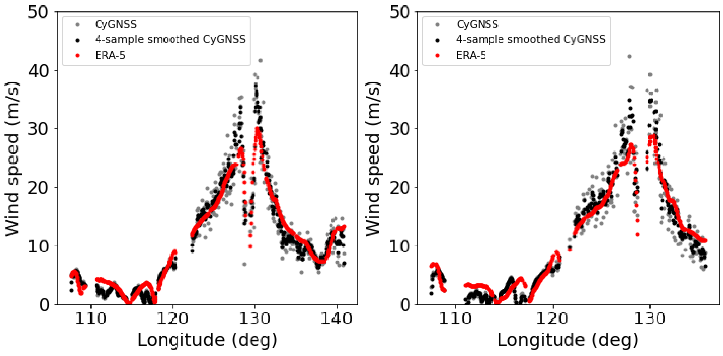
Figure 1. CyGNSS passes acquired during the typhoon ‘Trami’ in 29 September 2018, geographically close to the eye of the cyclone and within hours of the acquisition of a Sentinel SAR wind speed images—as shown in Figure A1, Appendix B. Our 1 Hz CyGNSS wind retrievals are plotted in grey dots (black dots after four sample–∼28 km–smoothing). The red dots are for ECMWF/C3S ERA5 wind speeds interpolated to the CyGNSS tracks. The tracks correspond to CyGNSS satellite numbers/track identification numbers: 01/722 (left) and 06/703 (right).
Remotesensing 12 03930 g001
Figure 2. Intermediate parameters in the processing of the CyGNSS tracks presented in Figure 1, one column each. (Top): observed, modelled, and calibrated signal peak to noise S o (grey), S m o d (red), and S o c a l (black), respectively. (Centre): ratio between the modelled and observed signal peak to noise r = S m o d / S o (grey) and the linear fit p (black). (Bottom): sensitivity H / x | x b . In both cases, the eye of the hurricane is at ∼130 longitude.
Remotesensing 12 03930 g002
Figure 3. Two-dimensional (2D) histogram of the correspondance between the CyGNSS retrievals obtained in this study and the ECMWF/C3S ERA5 wind speed values. The red line shows the 1:1 diagonal, the green line is a linear fit (parameters of the fit displayed in the title), the blue and orange dots correspond to 5 m/s-batched means ( < x c y g n s s > , < x e r a 5 > ), and their errorbars indicate ± their standard deviation (2 σ dispersion around the mean). Batches that are populated with more/less than 100 samples are plotted in blue/orange, respectively.
Remotesensing 12 03930 g003
Figure 4. Statistics of satellite observations with respect to ERA5 wind estimates, in batches of 5 m/s. Dots that are connected with lines correspond to the mean M = < O b s s a t E R A 5 > w i n d o w , with dispersion given by its standard deviation (crosses). Different colors are used for different satellite observations, and for windows with statistically significant ( N > 100 ) or non-significant ( N < 100 ) number of samples: black and grey for our CyGNSS retrievals (statistically significant and non-significant, respectively), red and pink for SMAP-ERA5, blue and cyan for SMOS-ERA5, green and lime for ASCAT_A-ERA5, and orange and yellow for ASCAT_B-ERA5.
Remotesensing 12 03930 g004
Figure 5. 2D histograms of the correspondance between the CyGNSS retrievals obtained in this study and different spaceborne wind sensors. The red line shows the 1:1 diagonal, the green line is a linear fit (parameters of the fit in the title), the dots with errorbars correspond to 5 m/s-batched means ( < x c y g n s s > , < x s e n s o r > ), and their errorbars indicate ± their standard deviation (2 σ dispersion around the mean). Only windows that are populated with more than 100 points are considered (blue) or between 10 and 100 (orange). (top-left): CyGNSS winds vs L-band radiometric SMAP wind retrievals. (top-right): CyGNSS winds vs L-band radiometric SMOS wind retrievals. (bottom-left): CyGNSS winds vs C-band scatterometer ASCAT-A wind measurements. (bottom-right): CyGNSS winds vs C-band scatterometer ASCAT-B wind measurements.
Remotesensing 12 03930 g005
Figure 6. (Top-Left): variational CyGNSS wind retrievals compared to the co-located SMAP wind retrievals, in batches of 5 m/s wind speeds (means shown in dots, ± σ in errorbars), grouped by IMERG rain rate values (color code). Different colors also used for batches with population statistically significant or not. (Top-Right): same for SMOS co-located with our CyGNSS wind retrievals. (Bottom): statistics between CyGNSS and ERA5, also grouped by rain rate.
Remotesensing 12 03930 g006
Figure 7. 2D Histograms of the comparison between our CyGNSS wind speed estimates (X-axis) and those provided by other organizations (Y-axis). (Top row): wind retrievals from the official CyGNSS data server, PODAAC (SDR Version 3.0), for FDS (left) and YSLF (right). The overall bias (standard deviation) are 1.1 m/s (3.2 m/s) and −13.8 m/s (9.9 m/s), respectively. (Bottom panel): CyGNSS wind retrievals from NOAA, with overall bias (standard deviation) −0.8 m/s (3.1 m/s). Superimposed to the histograms, the 1:1 diagonal (red line), the linear fit (green line), and batched mean and dispersion (dots with errorbars, blue when the number of samples in the batch exceeds 100, and orange when it does not reach 100 samples).
Remotesensing 12 03930 g007
Table 1. Set of criteria used to select or disregard CyGNSS data in this study, sorted by order of application.
Data Selection Criteria:
Removal of samples with receiver antenna gain in the specular direction <9 dBi
Track longer than 600 samples
Track with at least one sample where ERA5 wind speed >20 m/s
Removal of samples for which the location of the specular point is flagged as ‘land’ or ‘near land’
Track with more than 20% of samples with ERA5 wind speed between 5 and 25 m/s
Table 2. Main tropical cyclones across which this study found valid CyGNSS data. Number of tracks after quality check and selection criteria are applied, and that cover part of the area within the 34 kn (17.5 m/s) wind radii maximum extent as provided in the IBTrACS products [42] and averaged in the four cardinal directions.
PeriodTropical CyclonesNumber of Tracks
9 September 2018–29 September 2018Helene29
Mangkhut34
Florence24
Joyce3
Trami40
Leslie23
Rosa10
Kong-Rey1
26 August 2019–6 September 2019Dorian41
Juliette4
Lingling13
Gabrielle2
Faxai1
Table 3. Number of 1 Hz (2018 period) and 2 Hz (2019 period) CyGNSS wind speed retrievals co-located with other spaceborne wind retrievals, after all quality checks have been passed.
ERA5SMAPSMOSASCAT-AASCAT-b
308,646687011,92725,51424,931
Table 4. Comparison between ERA5 wind speed values and the satellite wind retrievals considered in this study, within windows of 5 m/s (first then rows) and using the whole set (bottom row). M = < O b s s a t E R A 5 > w i n d o w in m/s, σ = standard deviation in m/s and N is the number of observation in a given window. Note that, by definition, M takes positive values when the observations exceed the model. The values are presented in Figure 4.
RangeCyGNSSSMAPSMOSASCAT-AASCAT-B
M σ NM σ NM σ NM σ NM σ N
[0, 5)−0.72.270,363−0.71.8910−1.41.911120.31.437740.31.44830
[5, 10)−0.42.5139,3200.12.027200.92.053210.41.612,1220.31.611,554
[10, 15)−0.73.064,3321.01.920603.22.930000.41.767790.21.66138
[15, 20)0.32.824,3391.01.411354.24.814290.12.22496−0.22.12122
[20, 25)2.22.773601.91.6575.14.47500.93.17051.33.4950
[25, 30)4.63.020145.52.5178.15.12254.45.21773.76.1196
[30, 35)7.52.86496.70.41913.06.6376.32.8165.23.019
[35, 40)10.83.1207016.68.13108.31
[40, 45)15.13.041017.43.93400
[45, 50)21.63.711025.33.0900
All data−0.42.4308,6460.41.669182.23.911,9480.41.326,0690.31.325,810
Table 5. A comparison between the CyGNSS wind speed retrieved in this study and the other satellite wind retrievals, within windows of 5 m/s (like dots and errorbars and errorbars in Figure 5), and using the whole data set. The mean difference and dispersion at each window are provided (CyGNSS—other sensor, i.e., positive when CyGNSS retrievals exceed the other). The bottom row presents the Pearson’s correlation coefficient between our CyGNSS retrievals and these other sensors.
<CyGNSS—Other Spaceborne Sensed wind Speed >window (Dispersion) [m/s]
Window:SMAPSMOSASCAT-AASCAT-B
[0,5) m/s−1.2 (2.8)−4.5 (5.4)−1.2 (2.3)−1.2 (2.2)
[5,10) m/s−1.2 (2.9)−2.2 (4.1)−0.9 (2.4)−0.8 (2.5)
[10,15) m/s−0.4 (2.8)−1.7 (4.8)−0.7 (2.8)−0.9 (2.8)
[15,20) m/s0.4 (2.2)−3.3 (4.3)−0.2 (3.2)−0.5 (3.5)
[20,25) m/s0.7 (5.1)−1.7 (4.5)1.4 (3.3)1.0 (2.9)
[25,30) m/s0.2 (4.5)0.8 (9.5)2.9 (3.7)3.5 (2.7)
[30,35) m/s−0.7 (2.0)5.1 (9.3)5.3 (2.8)6.1 (2.8)
[35,40) m/s1.8 (–)9.8 (5.8)7.7 (2.5)8.5 (3.2)
[40,45) m/s19.5 (–)13.7 (1.4)12.3 (3.4)
[45,50) m/s31.6 (–)15.0 (–)
All data−0.8 (2.6)−2.5 (4.6)−0.8 (2.5)−0.8 (2.4)
Pearson’s Correlation Coefficient
All data0.830.650.860.88
Sample Availability: The variational CyGNSS wind retrievals are available from the authors.
Publisher’s Note: MDPI stays neutral with regard to jurisdictional claims in published maps and institutional affiliations.